The Geometry of Categorical and
Hierarchical Concepts in Large Language Models

Abstract

Understanding how semantic meaning is encoded in the representation spaces of large language models is a fundamental problem in interpretability. In this paper, we study the two foundational questions in this area. First, how are categorical concepts, such as $\{\texttt{mammal},\texttt{bird},\texttt{reptile},\texttt{fish}\}$, represented? Second, how are hierarchical relations between concepts encoded? For example, how is the fact that $\mathtt{dog}$ is a kind of $\mathtt{mammal}$ encoded? We show how to extend the linear representation hypothesis to answer these questions. We find a remarkably simple structure: simple categorical concepts are represented as simplices, hierarchically related concepts are orthogonal in a sense we make precise, and (in consequence) complex concepts are represented as polytopes constructed from direct sums of simplices, reflecting the hierarchical structure. We validate these theoretical results on the Gemma large language model, estimating representations for 957 hierarchically related concepts using data from WordNet. Code is available at github.com/KihoPark/LLM_Categorical_Hierarchical_Representations.

1 Introduction

This paper concerns how high-level semantic concepts are encoded in the representation spaces of large language models (LLMs). Understanding this is crucial for model interpretability and control. The ultimate aspiration is to monitor (and manipulate) the semantic behavior of LLMs (e.g., is the model’s response truthful) by directly measuring (and editing) the internal vector representations of the model [e.g.,][]li2023emergent, zou2023representation, ghandeharioun2024patchscope. Achieving this requires understanding how the geometric structure of the representation spaces corresponds to the high-level semantic concepts that humans understand. In this paper, we are concerned with two fundamental questions in this direction:

1. How are categorical concepts represented? For example, what is the representation of the concept $\texttt{animal}=\{\texttt{mammal},\texttt{bird},\texttt{reptile},\texttt{fish}\}$?

2. How are hierarchical relations between concepts represented? For example, what is the relationship between the representations of animal, mammal, dog, and poodle?

Our starting point is the linear representation hypothesis, the informal idea that high-level concepts are linearly encoded in the representation spaces of LLMs [e.g.,][]marks2023geometry, tigges2023linear, gurnee2024language. A main challenge for the linear representation hypothesis is that, in general, it’s not clear what “linear” means, nor what constitutes a “high-level concept”. park2024linear give a formalization in the limited setting of binary concepts that can be defined by counterfactual pairs of words. For example, the concept of $\texttt{male}\Rightarrow\texttt{female}$ is formalized using the counterfactual pairs $\{(\text{``man''},\text{``woman''}),(\text{``king''},\text{``queen''}),\dots\}$. They prove that such binary concepts have a well-defined linear representation as a direction in the representation space. They further connect semantic structure and representation geometry by showing that, under a causal inner product, concepts that can be freely manipulated (e.g., $\texttt{male}\Rightarrow\texttt{female}$ and $\texttt{french}\Rightarrow\texttt{english}$) are represented by orthogonal directions.

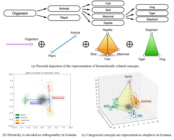
Figure 1: In large language models, categorical concepts are represented as simplices in the representation space. Further, hierarchically related concepts (such as $\mathtt{animal}$ and $\texttt{mammal}\Rightarrow\texttt{bird}$) live in orthogonal subspaces. The top panel illustrates the structure, the bottom panels show the measured representation structure in the Gemma LLM. See Section 5 for details.

Our aim is to extend this formalization beyond binary concepts represented as counterfactual word pairs. For example, the $\mathtt{animal}$ concept does not have a natural counterfactual definition, but such concepts are fundamental to human semantic understanding. Further, we aim to understand how the geometry of the representation space encodes relationships between concepts that cannot be freely manipulated, such as $\mathtt{animal}$ and $\mathtt{mammal}$.

To that end, we make the following contributions:

1. We show how to move from representations of binary concepts as directions to representations as vectors. This allows us to use vector operations to compose representations.

2. Using this result, we show that semantic hierarchy between concepts is encoded geometrically as orthogonality between representations, in a manner we make precise.

3. Then, we construct the representation of categorical variables (e.g., $\mathtt{animal}$) as the polytope where the vertices are the representations of the binary features that define the category (e.g., $\texttt{mammal},\texttt{bird},\dots$). We show that for “natural” concepts, the representation is a simplex.

4. Finally, we empirically validate these theoretical results on the Gemma large language model [][]team2024gemma. To that end, we extract concepts from the WordNet hierarchy [][]miller1995wordnet, estimate their representations, and show that the geometric structure of the representations align with the semantic hierarchy of WordNet.

The final structure is remarkably simple, and is summarized in Figure 1. In totality, these results provide a foundation for understanding how high-level semantic concepts are encoded in the representation spaces of LLMs.

2 Preliminaries

We begin with some necessary background.

2.1 Large Language Models

For the purposes of this paper, we consider a large language model to consist of two parts. The first part is a function $\lambda$ that maps input texts $x$ to vectors $\lambda(x)$ in a representation space $\Lambda\simeq\mathbb{R}^{d}$. This is the function given by the stacked transformer blocks. We take $\lambda(x)$ to be the output of the final layer at the final token position. The second part is an unembedding layer that assigns a vector $\gamma(y)$ in an unembedding space $\Gamma\simeq\mathbb{R}^{d}$ to each token $y$ in the vocabulary. Together, these define a sampling distribution over tokens via the softmax distribution:

$$\mathbb{P}(y\leavevmode\nobreak\ |\leavevmode\nobreak\ x)=\frac{\exp(\lambda(x)^{\top}\gamma(y))}{\sum_{y^{\prime}\in\mathrm{Vocab}}\exp(\lambda(x)^{\top}\gamma(y^{\prime}))}.$$ (2.1)

The broad goal is to understand how semantic structure is encoded in the geometry of the spaces $\Lambda$ and $\Gamma$. (We do not address the “internal” structure of the LLMs in this paper, though we are optimistic that a clear understanding of the softmax geometry will shed light on this as well.)

2.2 Concepts

We formalize a concept as a latent variable $W$ that is caused by the context $X$ and causes the output $Y$. That is, a concept is a thing that could—in principle—be manipulated to affect the output of the language model. In the particular case where a concept is a binary variable with a word-level counterfactual, we can identify the variable $W$ with the counterfactual pair of outputs $(Y(0),Y(1))$. Concretely, we can identify $\texttt{male}\Rightarrow\texttt{female}$ with $(Y(0),Y(1))\in_{R}\{(\text{``man''},\text{``woman''}),(\text{``king''},\text{``queen''}),(\text{``he''},\text{``her''}),\dots\}$. We emphasize that the notion of a concept as a latent variable that affects the output is more general than the counterfactual binary case.

Given a pair of concept variables $W$ and $Z$, we say that $W$ is causally separable with $Z$ if the potential outcome $Y(W=w,Z=z)$ is well-defined for all $w,z$. That is, two variables are causally separable if they can be freely manipulated—e.g., we can change the output language and the sex of the subject freely, so these concepts are causally separable.

2.3 Causal Inner Product and Linear Representations

We are trying to understand how concepts are represented. At this stage, there are two distinct representation spaces: $\Lambda$ and $\Gamma$. The former is the space of context embeddings, and the latter is the space of token unembeddings. We would like to unify these spaces so that there is just a single notion of representation.

park2024linear show how to achieve this unification via a “Causal Inner Product”. This is a particular choice of inner product that respects the semantics of language in the sense that the linear representations of (binary, counterfactual) causally separable concepts are orthogonal under the inner product. Their result can be understood as saying that there is some invertible matrix $A$ and constant vector $\bar{\gamma}_{0}$ such that, if we transform the embedding and unembedding spaces as

$$g(y)\leftarrow A(\gamma(y)-\bar{\gamma}_{0}),\quad\ell(x)\leftarrow A^{-\top}\lambda(x)$$ (2.2)

then the Euclidean inner product in the transformed spaces is the causal inner product, and the Riesz isomorphism between the embedding and unembedding spaces is simply the usual vector transpose operation. We can estimate $A$ as the whitening operation for the unembedding matrix. Following this transformation, we can think of the embedding and unembedding spaces as the same space, equipped with the Euclidean inner product.

Notice that the softmax probabilities are unchanged for any $A$ and $\bar{\gamma}_{0}$, so this transformation does not affect the model’s behavior. The vector $\bar{\gamma}_{0}$ defines an origin for the unembedding space, and can be chosen arbitrarily. We give a particularly convenient choice below.

In this unified space, the linear representation of a binary concept $W\in_{R}\{0,1\}$ is defined as:

Definition 1.

A vector $\bar{\ell}_{W}$ is a linear representation of a binary concept $W$ if for all contexts $\ell$, and all concept variables $Z$ that are causally separable with $W$, we have, for all $\alpha>0$,

$$\mathbb{P}(W=1\leavevmode\nobreak\ |\leavevmode\nobreak\ \ell+\alpha\bar{\ell}_{W}) >\mathbb{P}(W=1\leavevmode\nobreak\ |\leavevmode\nobreak\ \ell),\text{ and}$$ (2.3)

$$\mathbb{P}(Z\leavevmode\nobreak\ |\leavevmode\nobreak\ \ell+\alpha\bar{\ell}_{W}) =\mathbb{P}(Z\leavevmode\nobreak\ |\leavevmode\nobreak\ \ell).$$ (2.4)

That is, the linear representation is a direction in the representation space that, when added to the context, increases the probability of the concept, but does not affect the probability of any off-target concept. The representation is only a direction because $\alpha\bar{\ell}_{W}$ is also a linear representation for any $\alpha>0$ (i.e., there is no notion of magnitude). In the case of binary concepts that can be represented as counterfactual pairs of words, this direction can be shown to be proportional to the “linear probing” direction, and proportional to $g(Y(1))-g(Y(0))$ for any counterfactual pair $Y(1),Y(0)$ that differ on $W$.

3 Binary Concepts and Hierarchical Structure

Our high-level strategy will be to build up from binary concepts to more complex structure. We begin by defining the basic building blocks.

Binary and Categorical Concepts

We consider two kinds of binary concept. A binary feature $W\in_{R}\{\texttt{not\_w},\texttt{is\_w}\}$ is an indicator of whether the output has the attribute $w$. For example, if the feature $\mathtt{is\_animal}$ is true then the output will be about an animal. A binary contrast $\texttt{a}\Rightarrow\texttt{b}\in_{R}\{a,b\}$ is a binary variable that contrasts two specific attribute values. For example, the variable $\texttt{mammal}\Rightarrow\texttt{bird}$ is a binary contrast. In the particular case where the concept may be represented as counterfactual pairs of words, we can identify the contrast with the notion of linear representation in [PCV24].

We also define a categorical concept to be any concept corresponding to a categorical latent variable. This includes binary concepts as a special case.

Hierarchical Structure

The next step is to define what we mean by a hierarchical relation between concepts. To that end, to each attribute $w$, we associate a set of tokens $\mathcal{Y}(w)$ that have the attribute. For example, $\mathcal{Y}(\texttt{mammal})=\{\text{`` dog''},\text{`` cats''},\text{`` Tiger''},\dots\}$. Then,

Definition 2.

A value $z$ is subordinate to a value $w$ (denoted by $z\prec w$) if $\mathcal{Y}(z)\subseteq\mathcal{Y}(w)$. We say a categorical concept $Z\in_{R}\{z_{0},\dots,z_{k-1}\}$ is subordinate to a categorical concept $W\in_{R}\{w_{0},\dots,w_{n-1}\}$ if there exists a value $w_{Z}$ of $W$ such that each value $z_{i}$ of $Z$ is subordinate to $w_{Z}$.

For example, the binary contrast $\texttt{dog}\Rightarrow\texttt{cat}$ is subordinate to the binary feature $\{\texttt{is\_mammal},$ $\texttt{not\_mammal}\}$, and the binary contrast $\texttt{parrot}\Rightarrow\texttt{eagle}$ is subordinate to the categorical concept {$\mathtt{mammal}$, $\mathtt{bird}$, $\mathtt{fish}$}. On the other hand, $\texttt{dog}\Rightarrow\texttt{eagle}$ is not subordinate to $\texttt{bird}\Rightarrow\texttt{mammal}$, and $\texttt{bird}\Rightarrow\texttt{mammal}$ and $\texttt{live\_in\_house}\Rightarrow\texttt{live\_in\_water}$ are not subordinate to each other.

Linear Representations of Binary Concepts

Now we return to the question of how binary concepts are represented. A key desideratum is that if $\bar{\ell}_{W}$ is a linear representation then moving the representation in this direction should modify the probability of the target concept in isolation. If adding $\bar{\ell}_{W}$ also modified off-target concepts, it would not be natural to identify it with $W$. In Definition 1, this idea is formalized by the requirement that the probability of causally separable concepts is unchanged when the representation is added to the context.

We now observe that, when there is hierarchical structure, this requirement is not strong enough to capture ‘off-target’ behavior. For example, if $\bar{\ell}_{\texttt{animal}}$ captures the concept of animal vs not-animal, then moving in this direction should not affect the relative probability of the output being about a mammal versus a bird. If it did, then the representation would actually capture some amalgamation of the animal and mammal concepts. Accordingly, we must strengthen our definition:

Definition 3.

A vector $\bar{\ell}_{W}$ is a linear representation of a binary concept $W$ if

$$\mathbb{P}(W=1\leavevmode\nobreak\ |\leavevmode\nobreak\ \ell+\alpha\bar{\ell}_{W}) >\mathbb{P}(W=1\leavevmode\nobreak\ |\leavevmode\nobreak\ \ell)\text{, and}$$ (3.1)

$$\mathbb{P}(Z\leavevmode\nobreak\ |\leavevmode\nobreak\ \ell+\alpha\bar{\ell}_{W}) =\mathbb{P}(Z\leavevmode\nobreak\ |\leavevmode\nobreak\ \ell),$$ (3.2)

for all contexts $\ell$, all $\alpha>0$, and all concept variables $Z$ that are either subordinate or causally separable with $W$. Here, if $W$ is a binary feature for an attribute $w$, $W=1$ denotes $W=\texttt{is\_w}$.

Notice that, in the case of binary concepts defined by counterfactual pairs, this definition is equivalent to Definition 1, because such variables have no subordinate concepts.

4 Representations of Complex Concepts

We now turn to how complex concepts are represented. The high-level strategy is to show how to represent binary features as vectors, show how geometry encodes semantic composition, and then use this to construct representations of complex concepts.

4.1 Vector Representations of Binary Features

To build up to complex concepts, we need to understand how to compose representations of binary concepts. At this stage, the representations are directions in the representation space—they do not have a natural notion of magnitude. In particular, this means we cannot use vector operations (such as addition) to compose representations. To overcome this, we now show how to associate a magnitude to the representation of a binary concept.

The key is the following result, which connects binary feature representations and word unembeddings:

Theorem 4 (Magnitudes of Linear Representations).

Suppose there exists a linear representation (normalized direction) $\bar{\ell}_{W}$ of a binary feature $W$ for an attribute $w$. Then, there is a constant $b_{w}>0$ and a choice of unembedding space origin $\bar{\gamma}_{0}^{w}$ in eq. 2.2 such that

$$\begin{cases}\bar{\ell}_{W}^{\top}g(y)=b_{w}&\text{if }y\in\mathcal{Y}(w)\\ \bar{\ell}_{W}^{\top}g(y)=0&\text{if }y\not\in\mathcal{Y}(w).\end{cases}$$ (4.1)

Further, if there are $d$ causally separable attributes $\{w_{0},\dots,w_{d-1}\}$ with linear representations, we can choose a canonical origin $\bar{\gamma}_{0}$ in eq. 2.2 as

$$\bar{\gamma}_{0}=\sum_{i}\bar{\gamma}_{0}^{w_{i}}.$$ (4.2)

All proofs are given in Appendix A.

In words, this theorem says that if a (perfect) linear representation of the $\mathtt{animal}$ feature exists, then every token that has the animal attribute has the same dot product with the representation vector; i.e., “cat” is exactly as much $\mathtt{animal}$ as “dog” is. If this weren’t true, then increasing the probability that the output is about an animal would also increase the relative probability that the output is about a dog rather than a cat. In practice, such exact representations are unlikely to be found by gradient descent in LLM training. Rather, we expect $\bar{\ell}_{W}^{\top}g(y)$ to be isotropically distributed around $b_{w}$ with variance that is small compared to $b_{w}$ (so that animal and non-animal words are well-separated.)

With this result in hand, we can define a notion of vector representation for a binary feature:

Definition 5.

We say that binary feature $W$ for an attribute $w$ has a vector representation $\bar{\ell}_{w}\in\mathbb{R}^{d}$ if $\bar{\ell}_{w}$ satisfies Definition 3 and $\|\bar{\ell}_{w}\|_{2}=b_{w}$ in Theorem 4. If the vector representation of a binary feature is not unique, we say $\bar{\ell}_{w}$ is the vector representation that maximizes $b_{w}$.

4.2 Hierarchical Orthogonality

We have now moved from representations as directions to representations as vectors. Using this result, we now establish how hierarchical relations between concepts are encoded in the vector space structure of the representation space. The structure is illustrated in Figure 2. Formally, we have the following connections between vector and semantic structure:

Theorem 6 (Hierarchical Orthogonality).

Suppose there exist the vector representations for all the following binary features. Then, we have that

1. $\bar{\ell}_{w_{1}}-\bar{\ell}_{w_{0}}$ is a linear representation $\bar{\ell}_{w_{0}\Rightarrow w_{1}}$ defined in Definition 3;

2. $\bar{\ell}_{w}\perp\bar{\ell}_{z}-\bar{\ell}_{w}$ for $z\prec w$;

3. $\bar{\ell}_{w}\perp\bar{\ell}_{z_{1}}-\bar{\ell}_{z_{0}}$ for $Z\in_{R}\{z_{0},z_{1}\}$ subordinate to $W\in_{R}\{\texttt{not\_w},\texttt{is\_w}\}$;

4. $\bar{\ell}_{w_{1}}-\bar{\ell}_{w_{0}}\perp\bar{\ell}_{z_{1}}-\bar{\ell}_{z_{0}}$ for $Z\in_{R}\{z_{0},z_{1}\}$ subordinate to $W\in_{R}\{w_{0},w_{1}\}$; and

5. $\bar{\ell}_{w_{1}}-\bar{\ell}_{w_{0}}\perp\bar{\ell}_{w_{2}}-\bar{\ell}_{w_{1}}$ for $w_{2}\prec w_{1}\prec w_{0}$.

We emphasize that these results—involving differences of representations—are only possible because we now have vector representations (mere direction would not suffice).

4.3 Categorical Concepts as Simplices

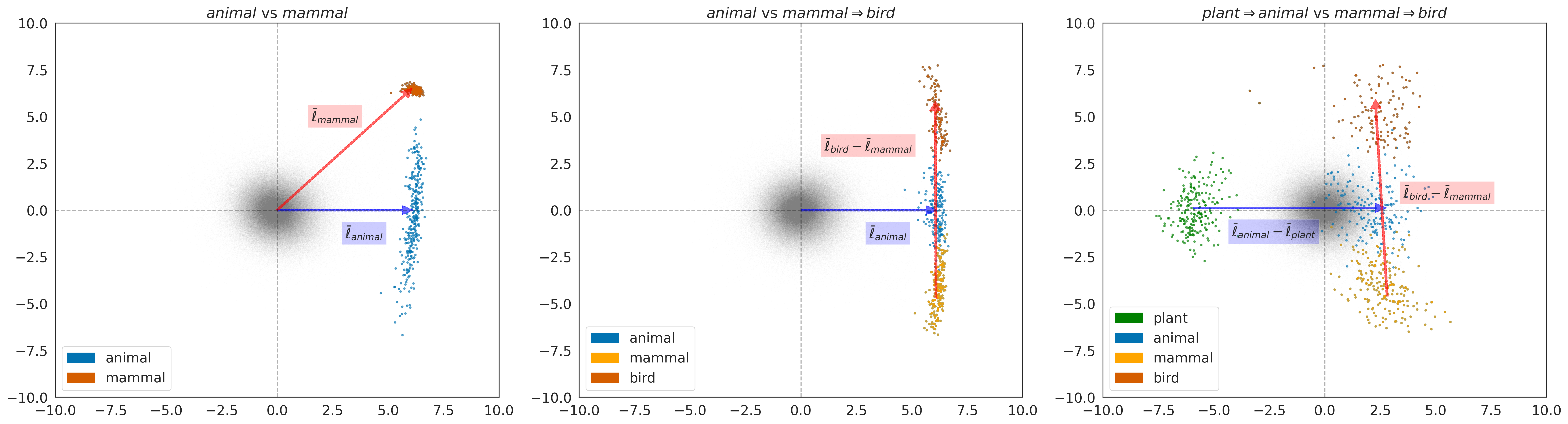
Figure 2: Hierarchical semantics are encoded as orthogonality in the representation space, as predicted in Theorem 6. The plots show the projection of the unembedding vectors on the 2D subspaces: $\mathrm{span}\{\bar{\ell}_{\texttt{animal}},\bar{\ell}_{\texttt{mammal}}\}$ (left; statement (b)), $\mathrm{span}\{\bar{\ell}_{\texttt{animal}},\bar{\ell}_{\texttt{bird}}-\bar{\ell}_{\texttt{mammal}}\}$ (middle; statement (c)), and $\mathrm{span}\{\bar{\ell}_{\texttt{animal}}-\bar{\ell}_{\texttt{plant}},\bar{\ell}_{\texttt{bird}}-\bar{\ell}_{\texttt{mammal}}\}$ (right; statement (d)). The gray points indicate all 256K tokens in the vocabulary, and the colored points are the tokens in $\mathcal{Y}(\texttt{w})$. The blue and red vectors are used to span the 2D subspaces.

The power of having a vector representation is that now we can use ordinary vector space operations to construct representation of other concepts. We now turn to the representation of categorical concepts, e.g., $\{\texttt{mammal},\texttt{reptile},\texttt{bird},\texttt{fish}\}.$ There is now a straightforward way to define the representation of such concepts:

Definition 7.

The polytope representation of a categorical concept $Z=\{z_{0},\dots,z_{k-1}\}$ is the convex hull of the vector representations of the elements of the concept.

Polytopes are quite general objects. The definition here also includes representations of categorical variables that are semantically unnatural, e.g., $\{\texttt{dog},\texttt{sandwich},\texttt{running}\}$. We would like to make a more precise statement about the representation of “natural” concepts. One possible notion of a “natural” concept is one where the model can freely manipulate the output values. The next theorem shows such concepts have particularly simple structure:

Theorem 8 (Categorical Concepts are Represented as Simplices).

Suppose that $\{w_{0},\dots,w_{k-1}\}$ is a collection of $k$ mutually exclusive attributes such that for every joint distribution $Q(w_{0},\dots w_{k-1})$ there is some $\ell_{i}$ such that $\mathbb{P}(W=w_{i}\leavevmode\nobreak\ |\leavevmode\nobreak\ \ell_{i})=Q(W=w_{i})$ for every $i$. Then, the vector representations $\bar{\ell}_{w_{0}},\dots,\bar{\ell}_{w_{k-1}}$ form a $(k-1)$-simplex in the representation space. In this case, we take the simplex to be the representation of the categorical concept $W=\{w_{0},\dots,w_{k-1}\}$.

Summary

Together, Theorems 6 and 8 give the simple structure illustrated in fig. 1: hierarchical concepts are represented as direct sums of simplices. The direct sum structure is immediate from the orthogonality in Theorem 6.

5 Experiments

We now turn to empirically testing the theoretical results in the representation space of the Gemma-2B large language model [][]team2024gemma.

5.1 Setup

Canonical representation space

The results in this paper rely on transforming the representation space so that the Euclidean inner product is a causal inner product, aligning the embedding and unembedding representations. Following [PCV24], we estimate the required transformation as:

$$g(y)=\mathrm{Cov}(\gamma)^{-1/2}(\gamma(y)-\mathbb{E}[\gamma])$$ (5.1)

where $\gamma$ is the unembedding vector of a word sampled uniformly from the vocabulary. Centering by $\mathbb{E}[\gamma]$ is a reasonable approximation of centering by $\bar{\gamma}_{0}$ defined in Theorem 4 because this makes the projection of a random $g(y)$ on an arbitrary direction close to $0$. This matches the requirement that the projection of a word onto a concept the words does not belong to should be close to $0$.

WordNet

We define a large collection of binary concepts using WordNet [][]miller1995wordnet. Briefly, WordNet organizes English words into a hierarchy of synsets, where each synset is a set of synonyms. The WordNet hierarchy is based on word hyponym relations, and reflects the semantic hierarchy of interest in this paper. We take each synset as an attribute $w$ and define $\mathcal{Y}(w)$ as the collection of all words belonging to any synset that is a descendant of $w$. For example, the synset mammal.n.01 is a descendant of animal.n.01, so both $\mathcal{Y}(\texttt{mammal.n.01})$ and $\mathcal{Y}(\texttt{animal.n.01})$ contain the word “dog”. We collect all noun and verb synsets, and augment the word collections by including plural forms of the nouns, multiple tenses of each verb, and capital and lower case versions of each word. We filter to include only those synsets with at least 50 words in the Gemma vocabulary. This leaves us with 593 noun and 364 verb synsets, each defining an attribute.

Estimation via Linear Discriminant Analysis

Now, we want to estimate the vector representation $\bar{\ell}_{w}$ for each attribute $w$. To do this, we make use of vocabulary sets $\mathcal{Y}(w)$. Following Theorem 4, the vector associated to the concept $w$ should have two properties. First, when the full vocabulary is projected onto this vector, the words in $\mathcal{Y}(w)$ should be well-separated from the rest of the vocabulary. Second, the projection of the unembedding vectors for $y\in\mathcal{Y}(w)$ should be approximately the same value. Equivalently, the variance of the projection of the unembedding vectors for $y\in\mathcal{Y}(w)$ should be small. To capture these requirements, we estimate the directions using a variant of Linear Discriminant Analysis (LDA), which finds a projection minimizing within-class variance and maximizing between-class variance. Formally, we estimate the vector representation of a binary feature $W$ for an attribute $w$ as

$$\bar{\ell}_{w}=\left(\tilde{g}_{w}^{\top}\mathbb{E}(g_{w})\right)\tilde{g}_{w},\quad\text{with}\quad\tilde{g}_{w}=\frac{\mathrm{Cov}(g_{w})^{\dagger}\mathbb{E}(g_{w})}{\|\mathrm{Cov}(g_{w})^{\dagger}\mathbb{E}(g_{w})\|_{2}},$$ (5.2)

where $g_{w}$ is the unembedding vector of a word sampled uniformly from $\mathcal{Y}(w)$ and $\mathrm{Cov}(g_{w})^{\dagger}$ is a pseudo-inverse of the covariance matrix. We estimate the covariance matrix $\mathrm{Cov}(g_{w})$ using the Ledoit-Wolf shrinkage estimator [][]ledoit2004well, because the dimension of the representation spaces is much higher than the number of samples.

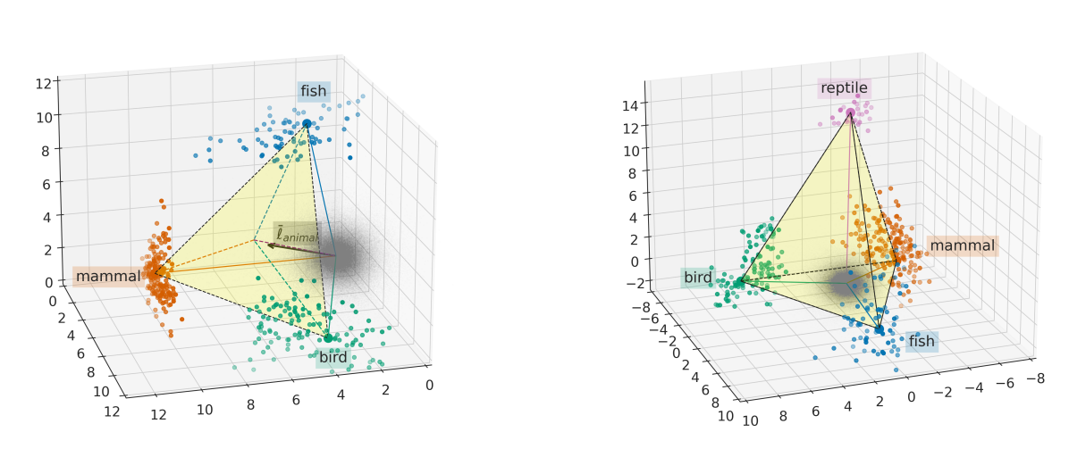
Figure 3: Categorical concepts are represented as simplices. The plots show the projection of the unembedding vectors on the 3D subspaces: $\mathrm{span}\{\bar{\ell}_{\texttt{mammal}},\bar{\ell}_{\texttt{bird}},\bar{\ell}_{\texttt{fish}}\}$ (left) and $\mathrm{span}\{\bar{\ell}_{\texttt{bird}}-\bar{\ell}_{\texttt{mammal}},\bar{\ell}_{\texttt{fish}}-\bar{\ell}_{\texttt{mammal}},\bar{\ell}_{\texttt{reptile}}-\bar{\ell}_{\texttt{mammal}}\}$ (right). The gray points indicate all 256K tokens in the vocabulary, and the colored points are the tokens in $\mathcal{Y}(\texttt{w})$. The left plot further shows the orthogonality between the triangle and the projection of $\bar{\ell}_{\texttt{animal}}$ (black arrow).

5.2 Visualization of $\mathtt{animal}$

As a concrete example, we check the theoretical predictions for the concept $\mathtt{animal}$. For this, we generated two sets of tokens $\mathcal{Y}(\texttt{animal})$ and $\mathcal{Y}(\texttt{plant})$ using ChatGPT-4 openai2023gpt4 and manually inspected them. $\mathcal{Y}(\texttt{animal})$ is separated to six sets of tokens for each subcategory $\{\texttt{mammal},\texttt{bird},\texttt{fish},\texttt{reptile},\texttt{amphibian},\texttt{insect}\}$.

Figure 2 illustrates the geometric relationships between various representation vectors. The main takeaway is that the semantic hierarchy is encoded as orthogonality in the manner predicted by Theorem 6. The figure also illustrates Theorem 4, showing that the projection of the unembedding vectors for $y\in\mathcal{Y}(w)$ is approximately constant, while the projection of $y\not\in\mathcal{Y}(w)$ is zero.

Figure 3 illustrates that the representation of a categorical concept is a simplex, as predicted in Theorem 8. It also shows that, as predicted, the simplex for $\texttt{fish},\texttt{mammal},\texttt{bird}$ is orthogonal to the vector representation of $\mathtt{animal}$.

5.3 WordNet Hierarchy

We now turn to using the WordNet hierarchy to evaluate the theoretical predictions at scale. We report the noun hierarchy here and defer the verb hierarchy to Appendix C.

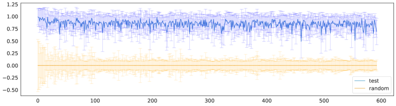
Figure 4: Linear representations exist for most binary features in the WordNet noun hierarchy. Comparison of projection of test and random words on estimated vector representations for each WordNet feature. The values are divided by the norm of the estimated vector representation. The $x$-axis indices denote all features in the noun hierarchy. The thick lines present the mean of the projections for each feature and the error bars indicate the 1.96 $\times$ standard error.

Existence of Vector Representations for Binary Features

To evaluate whether vector representations exist, for each synset $w$ we split $\mathcal{Y}(w)$ into train words (80%) and test words (20%), fit the LDA estimator to the train words, and examine the projection of the unembedding vectors for the test words onto the estimated vector representation. Figure 4 shows the mean and standard error of the test projections, divided by the magnitude of each estimated $\bar{\ell}_{w}$. If a vector representation exists for an attribute, we would expect these values to be close to 1. We see that this is indeed the case, giving evidence that vector representations do indeed exist for these features.

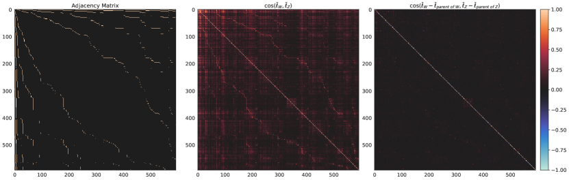
Figure 5: Hierarchical semantics in WordNet are encoded in Gemma representation space, with the orthogonal structure predicted in Theorem 6. The adjacency matrix of the hierarchical relations between features in the noun hierarchy (left), the cosine similarity between the vector representations $\bar{\ell}_{w}$ for each feature (middle), and the cosine similarity between child-parent vectors $\bar{\ell}_{w}-\bar{\ell}_{\text{parent of }w}$ for each feature (right). The features are ordered by the hierarchy.

Hierarchical Orthogonality

It remains to evaluate the prediction that hierarchical relations are encoded as orthogonality in the representation space. Figure 5 shows the adjacency matrix of the WordNet noun hyponym inclusion graph (left), the cosine similarity between the vector representations $\bar{\ell}_{w}$ for each feature (middle), and the cosine similarity between child-parent vectors $\bar{\ell}_{w}-\bar{\ell}_{\text{parent of }w}$ for each feature (right). Strikingly, the cosine similarity clearly reflects the semantic hierarchy—the adjacency matrix is clearly visible in the middle heatmap. This is because, e.g., $\mathtt{mammal.n.01}$ and $\mathtt{animal.n.01}$ have high cosine similarity. By contrast, as predicted by Theorem 6, the child-parent and parent-grandparent vectors are orthogonal. This also straightforwardly implies all other theoretical connections between orthogonality and semantic hierarchy.

In Appendix C, we present zoomed-in heatmaps for the subtree of descendants of “animal”, and the results for the verb hierarchy.

6 Discussion and Related Work

We set out to understand how semantic structure is encoded in the geometry of representation space. We have arrived an astonishingly simple structure, summarized in Figure 1. The key contributions are moving from representing concepts as directions to representing them as vectors (and polytopes), and connecting semantic hierarchy to orthogonality.

Related work

The results here connect closely to the study of linear representations in language models [MYZ13, PSM14, Aro+16, Elh+22, Bur+22, Tig+23, NLW23, Mos+22, Li+23a, Gur+23, Wan+23, Jia+24, PCV24, e.g.,]. In particular, [PCV24] formalize the linear representation hypothesis by unifying three distinct notions of linearity: word2vec-like embedding differences, logistic probing, and steering vectors. Our work relies on this unification, and just focuses on the steering vector notion. Our work also connects to work aimed at theoretically understanding the existence of linear representations. Specifically, [Aro+16, Aro+18, FG19] use RAND-WALK model where the latent vectors are modeled to drift on the unit sphere. [BL06, Rud+16, RB17] consider a similar dynamic topic modeling. [GAM17] and subsequent works [AH19, ABH19] propose a paraphrasing model where a subset of words is semantically equivalent to a single word. [EDH18] try to explain linear representations by decomposing the pointwise mutual information matrix while [RLV23] connect it to contrastive loss. jiang2024origins connect the existence of linear representations to the implicit bias of gradient descent. In this paper, we do not seek to justify the existence of linear representations, but rather to understand their structure if they do exist. Though, by empirically estimating vector representations for thousands of concepts, we add to the body of evidence supporting the existence of linear representations. [Elh+22] also empirically observe the formation of polytopes in the representation space of a toy model, and the present work can be viewed in part as giving an explanation for this phenomenon.

There is also a growing literature studying the representation geometry of natural language [MT17, Rei+19, VM21, VM20, Li+20, Che+21, CTB22, Lia+22, JAV23, Wan+23, PCV24, Val+24]. Much of this work focuses on connections to hyperbolic geometry [NK17, GBH18, Che+21, He+24]. We do not find such a connection in existing LLMs, but it is an interesting direction for future work to determine if more efficient LLM representations could be constructed in hyperbolic space. jiang2023uncovering hypothesize that very general "independence structures" are naturally represented by partial orthogonality in vector spaces [AAZ22]. The results here confirm and expand on this hypothesis in the case of hierarchical structure in language models.

Implications and Future Work

The results in this paper are foundational for understanding the structure of representation space in language models. Of course, the ultimate purpose of foundations is to build upon them. One immediate direction is to refine the attempts to interpret LLM structure to explicitly account for hierarchical semantics. As a concrete example, there is currently significant interest in using sparse autoencoders to extract interpretable features from LLMs [e.g.,][]cunningham2023sparse, bricken2023monosemanticity, attention_saes, braun2024identifying. This work searches for representations in terms of distinct binary features. Concretely, it hopes to find features for, e.g., $\mathtt{animal}$, $\mathtt{mammal}$, $\mathtt{bird}$, etc. Based on the results here, these representations are strongly co-linear, and potentially difficult to disentangle. On the other hand, a representation in terms of $\bar{\ell}_{\texttt{animal}}$, $\bar{\ell}_{\texttt{mammal}}-\bar{\ell}_{\texttt{animal}}$, $\bar{\ell}_{\texttt{bird}}-\bar{\ell}_{\texttt{animal}}$, etc., will be cleanly separated and equally interpretable. Fundamentally, semantic meaning has hierarchical structure, so interpretability methods should respect this structure. Understanding the geometric representation makes it possible to design such methods.

In a separate, foundational, direction: the results in this paper rely on using the canonical representation space. We estimate this using the whitening transformation of the unembedding layer. However, this technique only works for the final layer representation. It is an important open question how to make sense of the geometry of internal layers.

Appendix A Proofs

A.1 Proof of Theorem 4

See 4

Proof.

For any $y_{1},y_{0}\in\mathcal{Y}(w)$ or $y_{1},y_{0}\not\in\mathcal{Y}(w)$, let $Z$ be a binary concept where $\mathcal{Y}(Z=0)=\{y_{0}\}$ and $\mathcal{Y}(Z=1)=\{y_{1}\}$. Since $Z$ is subordinate to $W$, eq. 3.2 implies that

$$\operatorname*{logit}\mathbb{P}(Y=y_{1}\leavevmode\nobreak\ |\leavevmode\nobreak\ Y\in\{y_{0},y_{1}\},\ell+\bar{\ell}_{W})=\operatorname*{logit}\mathbb{P}(Y=y_{1}\leavevmode\nobreak\ |\leavevmode\nobreak\ Y\in\{y_{0},y_{1}\},\ell)$$ (A.1)

$$\iff\bar{\ell}_{W}^{\top}(g(y_{1})-g(y_{0}))=\bar{\ell}_{W}^{\top}A(\gamma(y_{1})-\gamma(y_{0}))=0$$ (A.2)

where $A$ is the invertible matrix in eq. 2.2. This means that $\bar{\ell}_{W}^{\top}A\gamma(y)$ is the same for all $y\in\mathcal{Y}(w)$, and it is also the same for all $y\not\in\mathcal{Y}(w)$.

Furthermore, for any $y_{1}\in\mathcal{Y}(w)$ and $y_{0}\not\in\mathcal{Y}(w)$, eq. 3.1 implies that

$$\operatorname*{logit}\mathbb{P}(Y=y_{1}\leavevmode\nobreak\ |\leavevmode\nobreak\ Y\in\{y_{0},y_{1}\},\ell+\bar{\ell}_{W})>\operatorname*{logit}\mathbb{P}(Y=y_{1}\leavevmode\nobreak\ |\leavevmode\nobreak\ Y\in\{y_{0},y_{1}\},\ell)$$ (A.3)

$$\iff\bar{\ell}_{W}^{\top}(g(y_{1})-g(y_{0}))=\bar{\ell}_{W}^{\top}A(\gamma(y_{1})-\gamma(y_{0}))>0.$$ (A.4)

Thus, by setting $b_{w}^{0}=\bar{\ell}_{W}^{\top}A\gamma(y)$ for any $y\not\in\mathcal{Y}(w)$, and $b_{w}=\bar{\ell}_{W}^{\top}A\gamma(y_{1})-\bar{\ell}_{W}^{\top}A\gamma(y_{0})>0$ for any $y_{1}\in\mathcal{Y}(w)$ and $y_{0}\not\in\mathcal{Y}(w)$, we get

$$\begin{cases}\bar{\ell}_{W}^{\top}A\gamma(y)=b_{w}^{0}+b_{w}&\text{if }y\in\mathcal{Y}(w)\\ \bar{\ell}_{W}^{\top}A\gamma(y)=b_{w}^{0}&\text{if }y\not\in\mathcal{Y}(w).\end{cases}$$ (A.5)

Then, we can choose an origin as

$$\bar{\gamma}_{0}^{w}=b_{w}^{0}A^{-1}\bar{\ell}_{W}$$ (A.6)

satisfying eq. 4.1.

On the other hand, if there exist $\bar{\ell}_{W}$ and $\bar{\ell}_{Z}$ for causally separable attributes $w$ and $z$, then $\bar{\ell}_{W}$ and $\bar{\ell}_{Z}$ are orthogonal by the property of the causal inner product. If they are not orthogonal, adding $\bar{\ell}_{Z}$ can change the other concept $W$, and it is a contradiction. Now if there exist the linear representation for $d$ binary features for causally separable attributes $\{w_{0},\dots,w_{d-1}\}$, we can choose a canonical $\bar{\gamma}_{0}$ in eq. 2.2 as

$$\bar{\gamma}_{0}=\sum_{i}\bar{\gamma}_{0}^{w_{i}}.$$ (A.7)

with eq. 4.1 satisfied. ∎

A.2 Proof of Theorem 6

See 6

Proof.

1. For $\bar{\ell}_{w_{1}}$ and $\bar{\ell}_{w_{0}}$, by Theorem 4, we have

   $$\begin{cases}(\bar{\ell}_{w_{1}}-\bar{\ell}_{w_{0}})^{\top}g(y)=0-b_{w_{0}}=-b_{w_{0}}&\text{if }y\in\mathcal{Y}(w_{0})\\ (\bar{\ell}_{w_{1}}-\bar{\ell}_{w_{0}})^{\top}g(y)=b_{w_{1}}-0=b_{w_{1}}&\text{if }y\in\mathcal{Y}(w_{1})\\ (\bar{\ell}_{w_{1}}-\bar{\ell}_{w_{0}})^{\top}g(y)=0-0=0&\text{if }y\not\in\mathcal{Y}(w_{0})\cup\mathcal{Y}(w_{1}).\end{cases}$$ (A.8)

   Since $\bar{\ell}_{w_{1}}-\bar{\ell}_{w_{0}}$ can change the target concept $w_{0}\Rightarrow w_{1}$ without changing any other concept subordinate or causally separable to the target concept, $\bar{\ell}_{w_{1}}-\bar{\ell}_{w_{0}}$ is the linear representation $\bar{\ell}_{w_{0}\Rightarrow w_{1}}$.

2. For $\bar{\ell}_{w}$ and $\bar{\ell}_{z}$ where $z\prec w$, by Theorem 4, we have

   $$\begin{cases}(\bar{\ell}_{z}-\bar{\ell}_{w})^{\top}g(y)=b_{z}-b_{w}&\text{if }y\in\mathcal{Y}(z)\\ (\bar{\ell}_{z}-\bar{\ell}_{w})^{\top}g(y)=0-b_{w}=-b_{w}&\text{if }y\in\mathcal{Y}(w)\setminus\mathcal{Y}(z)\\ (\bar{\ell}_{z}-\bar{\ell}_{w})^{\top}g(y)=0-0=0&\text{if }y\not\in\mathcal{Y}(w).\end{cases}$$ (A.9)

   When $w\setminus z$ denotes an attribute defined by $\mathcal{Y}(w)\setminus\mathcal{Y}(z)$, $\bar{\ell}_{z}-\bar{\ell}_{w}$ can change the target concept $w\setminus z\Rightarrow z$ without changing any other concept subordinate or causally separable to the target concept. Thus, $\bar{\ell}_{z}-\bar{\ell}_{w}$ is the linear representation $\bar{\ell}_{w\setminus z\Rightarrow z}$. This concept means $\texttt{not\_z}\Rightarrow\texttt{is\_z}$ conditioned on $w$, and hence it is subordinate to $w$.

   Therefore, $\bar{\ell}_{w}$ is orthogonal to the linear representation $\bar{\ell}_{w\setminus z\Rightarrow z}=\bar{\ell}_{z}-\bar{\ell}_{w}$ by the property of the causal inner product. If they are not orthogonal, adding $\bar{\ell}_{w}$ can change the other concept $w\setminus z\Rightarrow z$, and it is a contradiction.

3. By the above result (b), $\bar{\ell}_{w}^{\top}(\bar{\ell}_{z_{1}}-\bar{\ell}_{w})=\bar{\ell}_{w}^{\top}(\bar{\ell}_{z_{0}}-\bar{\ell}_{w})=0$. Therefore, $\bar{\ell}_{w}^{\top}(\bar{\ell}_{z_{1}}-\bar{\ell}_{z_{0}})=0$.

4. Let’s say that $w_{1}$ is $w_{Z}$ defined in Definition 2. The binary contrast $z_{0}\Rightarrow z_{1}$ is subordinate to the binary feature for the attribute $w_{0}$. By the property of the causal inner product, $\bar{\ell}_{w_{0}}$ is orthogonal to the linear representation $\bar{\ell}_{z_{0}\Rightarrow z_{1}}=\bar{\ell}_{z_{1}}-\bar{\ell}_{z_{0}}$ (by (a)). Then, with the above result (c), we have $(\bar{\ell}_{w_{1}}-\bar{\ell}_{w_{0}})^{\top}(\bar{\ell}_{z_{1}}-\bar{\ell}_{z_{0}})$.

5. By the above result (b), we have

   $$\begin{cases}\|\bar{\ell}_{w_{1}}-\bar{\ell}_{w_{0}}\|_{2}^{2}=\|\bar{\ell}_{w_{1}}\|_{2}^{2}-\|\bar{\ell}_{w_{0}}\|_{2}^{2}\\ \|\bar{\ell}_{w_{2}}-\bar{\ell}_{w_{1}}\|_{2}^{2}=\|\bar{\ell}_{w_{2}}\|_{2}^{2}-\|\bar{\ell}_{w_{1}}\|_{2}^{2}\\ \|\bar{\ell}_{w_{2}}-\bar{\ell}_{w_{0}}\|_{2}^{2}=\|\bar{\ell}_{w_{2}}\|_{2}^{2}-\|\bar{\ell}_{w_{0}}\|_{2}^{2}.\end{cases}$$ (A.10)

   Then,

   $$\|\bar{\ell}_{w_{1}}-\bar{\ell}_{w_{0}}\|_{2}^{2}+\|\bar{\ell}_{w_{2}}-\bar{\ell}_{w_{1}}\|_{2}^{2}$$ (A.11)

   $$=\|\bar{\ell}_{w_{1}}\|_{2}^{2}-\|\bar{\ell}_{w_{0}}\|_{2}^{2}+\|\bar{\ell}_{w_{2}}\|_{2}^{2}-\|\bar{\ell}_{w_{1}}\|_{2}^{2}$$ (A.12)

   $$=\|\bar{\ell}_{w_{2}}\|_{2}^{2}-\|\bar{\ell}_{w_{0}}\|_{2}^{2}$$ (A.13)

   $$=\|\bar{\ell}_{w_{2}}-\bar{\ell}_{w_{0}}\|_{2}^{2}.$$ (A.14)

   Therefore, $\bar{\ell}_{w_{1}}-\bar{\ell}_{w_{0}}$ is orthogonal to $\bar{\ell}_{w_{2}}-\bar{\ell}_{w_{1}}$.

∎

A.3 Proof of Theorem 8

See 8

Proof.

If we can represent arbitrary joint distributions, this means, in particular, that we can change the probability of one attribute without changing the relative probability between a pair of other attributes. Consider the case where $k=3$, as illustrated in Figure 6. If $\bar{\ell}_{w_{0}},\bar{\ell}_{w_{1}},\bar{\ell}_{w_{2}}$ are on a line, then there is no direction in that line (to change the value in the categorical concept) such that adding the direction can change the probability of $w_{2}$ without changing the relative probabilities between $w_{0}$ and $w_{1}$. However, if $\bar{\ell}_{w_{0}},\bar{\ell}_{w_{1}},\bar{\ell}_{w_{2}}$ are not on a line, they form a triangle. Then, there exists a line that is toward $\bar{\ell}_{w_{2}}$ and perpendicular to the opposite side of the triangle. Now adding the direction $\tilde{\ell}$ can manipulate the probability of $w_{2}$ without changing the relative probabilities between $w_{0}$ and $w_{1}$. That is, for any $\alpha>0$ and context embedding $\ell$,

$$\begin{cases}\mathbb{P}(W=w_{2}\leavevmode\nobreak\ |\leavevmode\nobreak\ \ell+\alpha\tilde{\ell})>\mathbb{P}(W=w_{2}\leavevmode\nobreak\ |\leavevmode\nobreak\ \ell),\text{ and}\\ \frac{\mathbb{P}(W=w_{1}\leavevmode\nobreak\ |\leavevmode\nobreak\ \ell+\alpha\tilde{\ell})}{\mathbb{P}(W=w_{0}\leavevmode\nobreak\ |\leavevmode\nobreak\ \ell+\alpha\tilde{\ell})}=\frac{\mathbb{P}(W=w_{1}\leavevmode\nobreak\ |\leavevmode\nobreak\ \ell)}{\mathbb{P}(W=w_{0}\leavevmode\nobreak\ |\leavevmode\nobreak\ \ell)}.\end{cases}$$ (A.15)

Therefore, the vectors $\bar{\ell}_{w_{0}},\bar{\ell}_{w_{1}},\bar{\ell}_{w_{2}}$ form a 2-simplex.

This argument extends immediately to higher $k$ by induction. For each $i\in\{0,\dots,k-1\}$, there should exist a direction that is toward $\bar{\ell}_{w_{i}}$ and orthogonal to the opposite hyperplane ($(k-2)$-simplex) formed by the other $\bar{\ell}_{w_{i^{\prime}}}$’s. Then, the vectors $\bar{\ell}_{w_{0}},\dots,\bar{\ell}_{w_{k-1}}$ form a $(k-1)$-simplex. ∎

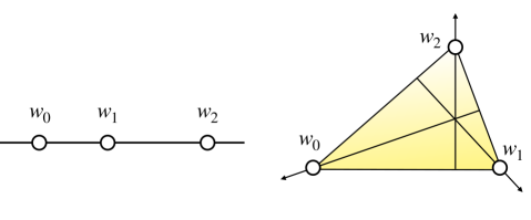
Figure 6: Illustration of the case $k=3$ in the proof of Theorem 8.

Appendix B Experiment Details

We employ the Gemma-2B version of the Gemma model [][]team2024gemma, which is accessible online via the huggingface library. Its two billion parameters are pre-trained on three trillion tokens. This model utilizes 256K tokens and 2,048 dimensions for the representation space.

We always use tokens that start with a space (‘$\backslash$u2581’) in front of the word, as they are used for next-word generation with full meaning. Additionally, like WordNet data we use, we include plural forms, and both capital and lowercase versions of the words in $\mathcal{Y}(\texttt{animal})$ and $\mathcal{Y}(\texttt{plant})$ for visualization in Section 5.2.

In the WordNet synset data, each content of the synset mammal.n.01 indicates that "mammal" is a word, "n" denotes "noun," and "01" signifies the first meaning of the word. In the WordNet hierarchy, if a parent has only one child, we combine the two features into one. Additionally, since the WordNet hierarchy is not a perfect tree, a child can have more than one parent. We use one of the parents when computing the $\bar{\ell}_{w}-\bar{\ell}_{\text{parent of }w}$.

Appendix C Additional Results

C.1 Zooming in on a Subtree of Noun Hierarchy

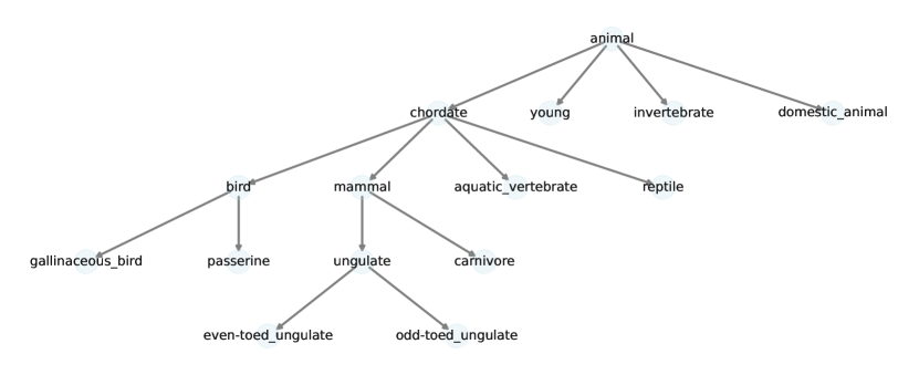
Figure 7: Subtree in WordNet noun hierarchy for descendants of animal.

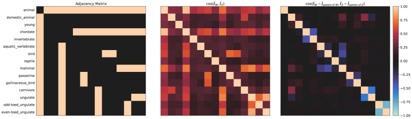
Figure 8: Zoomed-in Heatmaps of the subtree for animal in Figure 7.

As it is difficult to understand the entire WordNet hierarchy at once from the heatmaps in Figure 5, we present a zoomed-in heatmap for the subtree (Figure 7) for the feature animal in Figure 8. The left heatmap displays the adjacency matrix of the hierarchical relations between features, aligned with the subtree in Figure 7. The middle heatmap shows that the cosine similarities between the vector representations $\bar{\ell}_{w}$ correspond to the adjacency matrix. The final heatmap demonstrates that the child-parent vector $\bar{\ell}_{w}-\bar{\ell}_{\text{parent of }w}$ and $\bar{\ell}_{\text{parent of }w}-\bar{\ell}_{\text{grandparent of }w}$ are orthogonal, as predicted in Theorem 6.

C.2 WordNet Verb Hierarchy

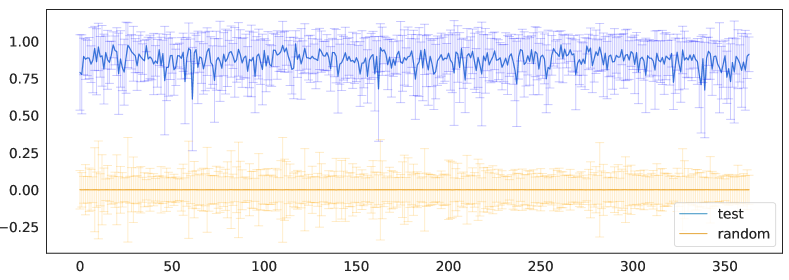
Figure 9: Linear representations exist for most binary features in the WordNet verb hierarchy. Comparison of projection of test and random words on estimated vector representations for each feature. The values are divided by the norm of the estimated vector representation. The $x$-axis indices denote all features in the verb hierarchy. The thick lines present the mean of the projections for each feature and the error bars indicate the 1.96 $\times$ standard error.

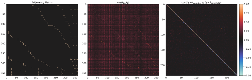
Figure 10: The adjacency matrix of the hierarchical relations between features in the WordNet verb hierarchy (left), the cosine similarity between the vector representations $\bar{\ell}_{w}$ for each feature (middle), and the cosine similarity between child-parent vectors $\bar{\ell}_{w}-\bar{\ell}_{\text{parent of }w}$ for each feature (right). The features are ordered by the hierarchy.

In the same way as for the noun hierarchy, we estimate the vector representations for the WordNet verb hierarchy. To evaluate whether vector representations exist, we split $\mathcal{Y}(w)$ for each synset $w$ into train words (80%) and test words (20%), fit the LDA estimator to the train words, and examine the projection of the unembedding vectors for the test words onto the estimated vector representation. Figure 9 shows the mean and standard error of the test projections, divided by the magnitude of each estimated $\bar{\ell}_{w}$. If a vector representation exists for an attribute, we would expect these values to be close to 1. This is indeed the case, providing evidence that vector representations do indeed exist for these features.

Figure 10 displays the adjacency matrix of the WordNet verb hyponym inclusion graph (left), the cosine similarity between the vector representations $\bar{\ell}_{w}$ for each feature (middle), and the cosine similarity between child-parent vectors $\bar{\ell}_{w}-\bar{\ell}_{\text{parent of }w}$ for each feature (right). The cosine similarity clearly reflects the semantic hierarchy—the adjacency matrix is clearly visible in the middle heatmap. By contrast, as predicted by Theorem 6, the child-parent and parent-grandparent vectors are orthogonal. This straightforwardly implies all other theoretical connections between orthogonality and the semantic hierarchy.

References

- [ABH19] Carl Allen, Ivana Balazevic and Timothy Hospedales “What the vec? Towards probabilistically grounded embeddings” In Advances in Neural Information Processing Systems 32, 2019
- [AH19] Carl Allen and Timothy Hospedales “Analogies explained: Towards understanding word embeddings” In International Conference on Machine Learning, 2019, pp. 223–231 PMLR
- [AAZ22] Arash A Amini, Bryon Aragam and Qing Zhou “A non-graphical representation of conditional independence via the neighbourhood lattice” In arXiv preprint arXiv:2206.05829, 2022
- [Aro+16] Sanjeev Arora et al. “A latent variable model approach to pmi-based word embeddings” In Transactions of the Association for Computational Linguistics 4 MIT Press One Rogers Street, Cambridge MA 02142-1209, USA journals-info …, 2016, pp. 385–399
- [Aro+18] Sanjeev Arora et al. “Linear algebraic structure of word senses, with applications to polysemy” In Transactions of the Association for Computational Linguistics 6, 2018, pp. 483–495
- [BL06] David M Blei and John D Lafferty “Dynamic topic models” In Proceedings of the 23rd international conference on Machine learning, 2006, pp. 113–120
- [Bra+24] Dan Braun, Jordan Taylor, Nicholas Goldowsky-Dill and Lee Sharkey “Identifying Functionally Important Features with End-to-End Sparse Dictionary Learning” In arXiv preprint arXiv:2405.12241, 2024
- [Bri+23] Trenton Bricken et al. “Towards Monosemanticity: Decomposing Language Models With Dictionary Learning” https://transformer-circuits.pub/2023/monosemantic-features/index.html In Transformer Circuits Thread, 2023
- [Bur+22] Collin Burns, Haotian Ye, Dan Klein and Jacob Steinhardt “Discovering latent knowledge in language models without supervision” In arXiv preprint arXiv:2212.03827, 2022
- [CTB22] Tyler A Chang, Zhuowen Tu and Benjamin K Bergen “The geometry of multilingual language model representations” In arXiv preprint arXiv:2205.10964, 2022
- [Che+21] Boli Chen et al. “Probing BERT in hyperbolic spaces” In arXiv preprint arXiv:2104.03869, 2021
- [Cun+23] Hoagy Cunningham et al. “Sparse autoencoders find highly interpretable features in language models” In arXiv preprint arXiv:2309.08600, 2023
- [Elh+22] Nelson Elhage et al. “Toy models of superposition” In arXiv preprint arXiv:2209.10652, 2022
- [EDH18] Kawin Ethayarajh, David Duvenaud and Graeme Hirst “Towards understanding linear word analogies” In arXiv preprint arXiv:1810.04882, 2018
- [FG19] Abraham Frandsen and Rong Ge “Understanding composition of word embeddings via tensor decomposition” In arXiv preprint arXiv:1902.00613, 2019
- [GBH18] Octavian Ganea, Gary Bécigneul and Thomas Hofmann “Hyperbolic entailment cones for learning hierarchical embeddings” In International Conference on Machine Learning, 2018, pp. 1646–1655 PMLR
- [Gha+24] Asma Ghandeharioun et al. “Patchscopes: A Unifying Framework for Inspecting Hidden Representations of Language Models” In International Conference on Machine Learning (to appear), 2024
- [GAM17] Alex Gittens, Dimitris Achlioptas and Michael W. Mahoney “Skip-Gram - Zipf + Uniform = Vector Additivity” In Annual Meeting of the Association for Computational Linguistics, 2017
- [Gur+23] Wes Gurnee et al. “Finding Neurons in a Haystack: Case Studies with Sparse Probing” In arXiv preprint arXiv:2305.01610, 2023
- [GT24] Wes Gurnee and Max Tegmark “Language Models Represent Space and Time” In The Twelfth International Conference on Learning Representations, 2024 URL: https://openreview.net/forum?id=jE8xbmvFin
- [He+24] Yuan He, Zhangdie Yuan, Jiaoyan Chen and Ian Horrocks “Language Models as Hierarchy Encoders” In arXiv preprint arXiv:2401.11374, 2024
- [JAV23] Yibo Jiang, Bryon Aragam and Victor Veitch “Uncovering meanings of embeddings via partial orthogonality” In arXiv preprint arXiv:2310.17611, 2023
- [Jia+24] Yibo Jiang et al. “On the Origins of Linear Representations in Large Language Models” In International Conference on Machine Learning (to appear), 2024
- [Kis+24] Connor Kissane, Robert Krzyzanowski, Arthur Conmy and Neel Nanda “Sparse Autoencoders Work on Attention Layer Outputs”, Alignment Forum, 2024 URL: https://www.alignmentforum.org/posts/DtdzGwFh9dCfsekZZ
- [LW04] Olivier Ledoit and Michael Wolf “A well-conditioned estimator for large-dimensional covariance matrices” In Journal of multivariate analysis 88.2 Elsevier, 2004, pp. 365–411
- [Li+20] Bohan Li et al. “On the sentence embeddings from pre-trained language models” In arXiv preprint arXiv:2011.05864, 2020
- [Li+23] Kenneth Li et al. “Emergent World Representations: Exploring a Sequence Model Trained on a Synthetic Task” In The Eleventh International Conference on Learning Representations, 2023
- [Li+23a] Kenneth Li et al. “Inference-Time Intervention: Eliciting Truthful Answers from a Language Model” In arXiv preprint arXiv:2306.03341, 2023
- [Lia+22] Victor Weixin Liang et al. “Mind the gap: Understanding the modality gap in multi-modal contrastive representation learning” In Advances in Neural Information Processing Systems 35, 2022, pp. 17612–17625
- [MT23] Samuel Marks and Max Tegmark “The geometry of truth: Emergent linear structure in large language model representations of true/false datasets” In arXiv preprint arXiv:2310.06824, 2023
- [Mes+24] Thomas Mesnard et al. “Gemma: Open models based on gemini research and technology” In arXiv preprint arXiv:2403.08295, 2024
- [MYZ13] Tomáš Mikolov, Wen-tau Yih and Geoffrey Zweig “Linguistic regularities in continuous space word representations” In Proceedings of the 2013 conference of the north american chapter of the association for computational linguistics: Human language technologies, 2013, pp. 746–751
- [Mil95] George A Miller “WordNet: a lexical database for English” In Communications of the ACM 38.11 ACM New York, NY, USA, 1995, pp. 39–41
- [MT17] David Mimno and Laure Thompson “The strange geometry of skip-gram with negative sampling” In Conference on Empirical Methods in Natural Language Processing, 2017
- [Mos+22] Luca Moschella et al. “Relative representations enable zero-shot latent space communication” In arXiv preprint arXiv:2209.15430, 2022
- [NLW23] Neel Nanda, Andrew Lee and Martin Wattenberg “Emergent Linear Representations in World Models of Self-Supervised Sequence Models” In arXiv preprint arXiv:2309.00941, 2023
- [NK17] Maximillian Nickel and Douwe Kiela “Poincaré embeddings for learning hierarchical representations” In Advances in neural information processing systems 30, 2017
- [Ope23] OpenAI “GPT-4 Technical Report” In arXiv preprint arXiv:2303.08774, 2023
- [PCV24] Kiho Park, Yo Joong Choe and Victor Veitch “The Linear Representation Hypothesis and the Geometry of Large Language Models” In International Conference on Machine Learning (to appear), 2024
- [PSM14] Jeffrey Pennington, Richard Socher and Christopher D Manning “Glove: Global vectors for word representation” In Proceedings of the 2014 conference on empirical methods in natural language processing (EMNLP), 2014, pp. 1532–1543
- [Rei+19] Emily Reif et al. “Visualizing and measuring the geometry of BERT” In Advances in Neural Information Processing Systems 32, 2019
- [RLV23] Narutatsu Ri, Fei-Tzin Lee and Nakul Verma “Contrastive Loss is All You Need to Recover Analogies as Parallel Lines” In arXiv preprint arXiv:2306.08221, 2023
- [RB17] Maja Rudolph and David Blei “Dynamic bernoulli embeddings for language evolution” In arXiv preprint arXiv:1703.08052, 2017
- [Rud+16] Maja Rudolph, Francisco Ruiz, Stephan Mandt and David Blei “Exponential family embeddings” In Advances in Neural Information Processing Systems 29, 2016
- [Tig+23] Curt Tigges, Oskar John Hollinsworth, Atticus Geiger and Neel Nanda “Linear representations of sentiment in large language models” In arXiv preprint arXiv:2310.15154, 2023
- [Val+24] Lucrezia Valeriani et al. “The geometry of hidden representations of large transformer models” In Advances in Neural Information Processing Systems 36, 2024
- [VM20] Riccardo Volpi and Luigi Malagò “Evaluating Natural Alpha Embeddings on Intrinsic and Extrinsic Tasks” In Workshop on Representation Learning for NLP, 2020
- [VM21] Riccardo Volpi and Luigi Malagò “Natural alpha embeddings” In Information Geometry 4.1 Springer, 2021, pp. 3–29
- [Wan+23] Zihao Wang, Lin Gui, Jeffrey Negrea and Victor Veitch “Concept Algebra for (Score-Based) Text-Controlled Generative Models” In Advances in Neural Information Processing Systems, 2023 URL: https://openreview.net/forum?id=SGlrCuwdsB
- [Zou+23] Andy Zou et al. “Representation engineering: A top-down approach to ai transparency” In arXiv preprint arXiv:2310.01405, 2023