Towards Universal Unfolding of Detector Effects in High-Energy Physics using Denoising Diffusion Probabilistic Models

Abstract

The unfolding of detector effects in experimental data is critical for enabling precision measurements in high-energy physics. However, traditional unfolding methods face challenges in scalability, flexibility, and dependence on simulations. We introduce a novel unfolding approach using conditional Denoising Diffusion Probabilistic Models (cDDPM). Our method utilizes the cDDPM for a non-iterative, flexible posterior sampling approach, which exhibits a strong inductive bias that allows it to generalize to unseen physics processes without explicitly assuming the underlying distribution. We test our approach by training a single cDDPM to perform multidimensional particle-wise unfolding for a variety of physics processes, including those not seen during training. Our results highlight the potential of this method as a step towards a “universal” unfolding tool that reduces dependence on truth-level assumptions.

1 Introduction

Unfolding detector effects in high-energy physics (HEP) events is a critical challenge with significant implications for both theoretical and experimental physics. Experimental data in HEP presents a distorted picture of the true physics processes due to detector effects. Unfolding is an inverse-problem solved through statistical inference that aims to correct the detector distortions of the observed data to recover the true distribution of particle properties. This process is essential for the validation of theories, new discoveries, precision measurements, and comparison of experimental results between different experiments. Since there are flaws in any possible solution to such a problem, the quality of the statistical inference directly impacts the reliability of scientific conclusions, making unfolding a cornerstone in high-energy physics research.

Traditional unfolding methods [5] are based on the linearization of the problem, reducing it to the resolution of a set of linear equations. Such approaches often suffer from limitations such as the requirement for data to be binned into histograms, the inability to unfold multiple observables simultaneously, and the lack of utilization of all features that control the detector response. These limitations necessitate a more robust and comprehensive approach to unfolding that would increase the usefulness of a dataset, for example by providing more information about the underlying physics process that led to the observed data.

Machine learning methods for unfolding have recently emerged as a powerful tool for this purpose. The ability of machine learning algorithms to learn patterns and relationships from large datasets makes them well-suited to analyzing the vast amounts of data generated by modern particle experiments. The OmniFold method, for instance, mitigates many of the challenges faced by traditional approaches by allowing us to utilize a multidimensional representation of the particles, which can include both the full phase space information and high-dimensional features [1]. Along with OmniFold, a variety of machine learning approaches for unfolding have been presented in recent years, including generative adversarial networks [9], conditional invertible neural networks [2], latent variational diffusion models [16], Schrödinger bridges and diffusion models [11], and others, see [15] for a recent survey. Each new method has made further strides in unfolding and shown the advantages in machine learning based approaches compared to traditional techniques. However, these methods all rely on an explicit description of the expected underlying distribution resulting from the unfolding process.

In this work, we introduce a novel approach based on Denoising Diffusion Probabilistic Models (DDPM) to unfold detector effects in HEP data without requiring an explicit assumption about the underlying distribution. We demonstrate how a single conditional DDPM can be trained to perform multidimensional particle-wise unfolding for a variety of physics processes. This flexibility is a step towards a “universal” unfolding tool, providing unfolded estimates while reducing the dependence on truth-level assumptions that could bias the results. This study serves as a benchmark for improving unfolding methods for the LHC and future colliders.

2 Unfolding

2.1 Posing the Unfolding Problem

The traditional approach to unfolding begins with a detailed model that describes how detector effects distort the particle property distributions. These distortions affect the kinematic quantities of particles incident to the detector, altering the distribution $f_{\text{true}}(x)$ that characterizes the underlying physics process. To reverse this distortion, statistical tools are used to infer this underlying distribution from the observed distribution $f_{\text{det}}(y)$ obtained from data. Mathematically, that amounts to solving a Fredholm integral equation of the first kind [4],

$$f_{\text{det}}(y)=\int{dx\,P(y|x)\,f_{\text{true}}(x)}$$ (1)

where $P(y|x)$ is the conditional probability distribution describing the detector effects. Unfolding requires the inverse process $P(x|y)$, which describes the probability of a particle with true value $x$ given a detector measurement $y$. With Bayes’ theorem, this conditional probability can be expressed as

$$P(x|y)=\frac{P(y|x)f_{\text{true}}(x)}{f_{\text{det}}(y)}~{}.$$ (2)

In this context, a detector dataset can be unfolded by sampling from the posterior $P(x|y)$ to recover the distribution $f_{\text{true}}(x)$. Since the detector effects $P(y|x)$ are assumed to be the same for any physics distribution, we can see that the posterior $P(x|y)$ depends on the prior distribution $f_{\text{true}}(x)$. Therefore, if we approximate $P(x|y)$ using a dataset for a specific physics process described by $f_{\text{true}}(x)$, then this posterior $P(x|y)$ will only serve to unfold detector data for physics processes that also follow $f_{\text{true}}(x)$.

This reveals one of the main challenges in developing a universal unfolder, which can be applied to unfold detector data for any physics process. Instead of developing a method able to learn a posterior $P(x|y)$ to unfold detector data pertaining to a specific true underlying distribution, a universal unfolder aims to remove detector effects from any set of measured data agnostic of the process of interest, ideally with no bias towards any prior distribution.

2.2 Our Unfolding Approach

Although we cannot achieve an ideal universal unfolder, we can seek an approach that will enhance the inductive bias of the unfolding method to improve generalization to cover various posteriors pertaining to different physics data distributions. From eq. 2 we can see that the posteriors for two different physics processes $i$ and $j$ are related by a ratio of the probability density functions of each process,

$$\frac{P_{i}(x|y)}{P_{j}(x|y)}=\frac{f_{\text{true}}^{\,i}(x)\,f_{\text{det}}^{\,j}(y)}{f_{\text{det}}^{\,i}(y)\;f_{\text{true}}^{\,j}(x)}~{}.$$ (3)

Assuming we can learn the posterior for a given physics process, we note that we could extrapolate to unseen posteriors if the priors $f_{\text{true}}(x)$ and detector distributions $f_{\text{det}}(y)$ can be approximated or written in a closed form. Although these functions have no analytical form, we can approximate key features using the first moments of these distributions. By making use of these moments, we can have a more flexible unfolder that is not strictly tied to a selected prior distribution, and enables it to interpolate and extrapolate to unseen posteriors based on the provided moments. Consequently, this unfolding tool gains the ability to handle a wider range of physics processes and enhances the generalization capabilities, making it a more versatile tool for unfolding in various high energy physics applications.

In practice, one can use a training dataset of pairs $\{x,y\}$ to train a machine learning model to learn a posterior $P(x|y)$. To implement our approach and improve the inductive bias, we define a training dataset consisting of multiple prior distributions and incorporate the moments of these distributions to the data pairs. The moments are therefore included in the conditioning and generative aspects of the machine learning model such that it may be able to model multiple posteriors. As a result, we establish an unfolding tool as a posterior sampler that, when trained with sufficient priors within a family of distributions, is “universal” in the sense that it has a strong inductive bias to allow generalization towards estimating the prior distribution of unseen datasets. Further details and a technical description of this method are provided in section 4.

Our proposed approach calls for a flexible generative model, and denoising diffusion probabilistic models (DDPMs) [13] lend themselves naturally to this task. DDPMs learn via a reversible generative process that can be conditioned directly on the moments of the distribution $f_{\text{det}}(y)$ and on the detector values themselves, providing a natural way to model $P(x|y)$ for unfolding. In particular, the various conditioning methods available for DDPMs offer the flexibility to construct a model that can adapt to different detector data distributions and physics processes. Further details on DDPMs are provided in section 3.

3 Denoising Diffusion Probabilistic Models

The standard DDPM [13] consists of two parts. First is a forward process (or diffusion process) $q(x_{t}|x_{t-1})$ which is fixed to a Markov chain that gradually adds Gaussian noise (following a variance schedule $\beta_{1},...,\beta_{T}$) to data samples from a known initial distribution,

$$q(x_{t}|x_{t-1}):=\mathcal{N}(x_{t}\,;\sqrt{1-\beta_{t}}\,x_{t},\;\beta_{t}\,\mathbf{I}).$$ (4)

Second is a learned reverse process (or denoising process) $p_{\theta}\,(x_{0:T})$ parameterized by $\theta$. The reverse process is also a Markov chain with learned Gaussian transitions starting at $p(x_{T})=\mathcal{N}(x_{T};\mathbf{0},\mathbf{I})$,

$$p_{\theta}\,(x_{0:T}):=p(x_{T})\prod^{T}_{t=1}p_{\theta}\,(x_{t-1}|x_{t})$$ (5)

$$p_{\theta}(x_{t-1}|x_{t}):=\mathcal{N}\bigl{(}x_{t-1}\,;\mu_{\theta}(x_{t},t),\;\sigma_{t}^{2}\mathbf{I}\bigr{)}.$$ (6)

By learning to reverse the forward diffusion process, the model learns meaningful latent representations of the underlying data and is able to remove noise from data to generate new samples from the associated data distribution. This type of generative model has natural applications in high energy physics, for example generating data samples from known particle distributions. However, to be used in unfolding the process must be altered so that the denoising procedure is dependent on the observed detector data, $y$. This can be achieved by incorporating conditioning methods to the DDPM.

3.1 Conditional DDPM

Conditioning methods for DDPMs can either use conditions to guide unconditional DDPMs in the reverse process [7], or they can incorporate direct conditions to the learned reverse process. While guided diffusion methods have had great success in image synthesis [10], direct conditioning provides a framework that is particularly useful in unfolding.

We implement a conditional DDPM (cDDPM) for unfolding that keeps the original unconditional forward process and introduces a simple, direct conditioning on $y$ to the reverse process,

$$p_{\theta}\,(x_{0:T}|y):=p(x_{T}|y)\prod^{T}_{t=1}p_{\theta}\,(x_{t-1}|x_{t},y).$$ (7)

Similar to an unconditional DDPM, this reverse process has the same functional form as the forward process and can be expressed as a Gaussian transition with a learned mean $\mu_{\theta}$ and a fixed variance at each timestep $\sigma^{2}_{t}$,

$$p_{\theta}(x_{t-1}|x_{t},y):=\mathcal{N}\bigl{(}x_{t-1}\,;\mu_{\theta}(x_{t},y),\;\sigma_{t}^{2}\mathbf{I}\bigr{)}.$$ (8)

This conditioned reverse process learns to directly estimate the posterior probability $P(x|y)$ through its Gaussian transitions. More specifically, the reverse process, parameterized by $\theta$, learns to remove the introduced noise to recover the target value $x$ by conditioning directly on $y$.

Training optimizes the parameters $\theta$ to maximize the likelihood of accurately estimating the noise $\epsilon$ that should be removed at each timestep in order to denoise $x_{t}$ given the condition $y$. Similar to the unconditional DDPM, we use the Gaussian nature of these transitions and a reparametrization of the mean to simplify the loss function to the mean squared error (MSE) between the noise $\epsilon$ added at each timestep during the forward process and the noise $\epsilon_{\theta}(x_{t},y)$ predicted by the model given the noisy sample $x_{t}$ at timestep $t$ and the condition $y$:

$$L(\theta)=\mathbb{E}_{\epsilon,x_{t},y}\left[\Big{\|}\epsilon-\epsilon_{\theta}\,(x_{t},y)\Big{\|}^{2}\right].$$ (9)

A detailed derivation of this loss can be found in Appendix A. We can compare this approach to the commonly used guided conditioning method, where the model estimates the noise with a weighted combination of the conditional and unconditional predictions as $\tilde{\epsilon}_{\theta,\phi}(x_{t},y)=(1+w)\,\epsilon_{\theta}(x_{t},y)-w\,\epsilon_{\phi}(x_{t})$ [14]. The cDDPM approach can be seen as a special case of guided conditioning with the guidance weight $w=0$. In this case, sampling would be done purely according to the learned conditional distribution $p_{\theta}(x_{t}|y)$. Although the learned conditional probability implicitly depends on the prior, sampling from the cDDPM does not require explicitly evaluating the prior distribution $p_{\phi}(x_{t})$ over the data space. This makes the cDDPM a natural choice for applications like unfolding where the prior is unknown or difficult to model.

4 Unfolding with cDDPMs

This section describes how we use the cDDPM formulation to approach the problem of universal unfolding in two parts: (a) using vector data pairs $(\vec{x},\vec{y})$ from a physics simulation we can train a cDDPM to achieve multidimensional particle-wise unfolding by learning the posterior $P(\vec{x}|\vec{y})$ (section 4.1), (b) using simulated data for a variety of physics processes $i$ and imposing a conditioning based on the moments of the detector-level distributions, we can train a cDDPM to learn multiple posteriors $P_{i}(\vec{x}|\vec{y})$. During sampling, the model can then extrapolate to estimate an unseen $P_{j}(\vec{x}|\vec{y})$ of some other physics process $j$, thereby acting as a flexible unfolding tool that can generalize to unseen distributions (section 4.2). Finally, we describe the cDDPM architecture and present pseudocode for the training and sampling algorithms in section 4.3.

4.1 Multidimensional Particle-Wise Unfolding

The first step towards developing our unfolding tool is to setup a denoising diffusion process that can achieve multidimensional unfolding in a particle-wise manner. We setup a toy model and define particle kinematic information with a version of the 4-momentum vector that includes the transverse momentum, pseudorapidity, azimuthal angle, and energy of the particle ($[p_{T},\eta,\phi,E]$). These particle 4-vectors are defined both at truth-level as $\vec{x}$ and detector-level as $\vec{y}$. A cDDPM can be trained with data pairs $(\vec{x},\vec{y})$ as input to learn the posterior distribution $P(\vec{x}|\vec{y})$. When sampling, the model receives detector data $\vec{y}$ as input and conditionally generates the corresponding truth-level $\vec{x}$ according to $P(\vec{x}|\vec{y})$. This unfolding is done on a particle-by-particle basis, allowing the event-wise information to be preserved.

As described in section 3.1, the conditioning of the cDDPM is defined such that the sampling procedure is based solely on the posterior $P(\vec{x}|\vec{y})$ without explicit evaluation of the training data prior. Section 5.1 provides experimental results demonstrating this.

4.2 Generalization and Inductive Bias

Once we establish a cDDPM that can learn a posterior distribution $P(\vec{x}|\vec{y})$ for unfolding, we turn our attention to developing a tool that can unfold a variety of physics processes. As detailed in section 2.2, different physics processes will have different associated posteriors, and we aim to develop an unfolding tool with strong inductive bias to cover a wide range of these posteriors.

Since the posteriors $P_{i}(\vec{x}|\vec{y})$ depend on their respective prior $f_{\text{true}}^{\,i}(\vec{x})$ and detector distribution $f_{\text{det}}^{\,i}(\vec{y})$, adding information that describes these distributions may enable the cDDPM to gain a flexibility to learn various $P_{i}(\vec{x}|\vec{y})$. We choose to use the moments of the particle $p_{T}$ distribution of $f_{\text{true}}^{\,i}(\vec{x})$ and $f_{\text{det}}^{\,i}(\vec{y})$, since the $p_{T}$ distribution is a distinguishing feature for a physics process. For each simulated physics process $i$ we calculate the first six moments of $\{x_{p_{T}}\}_{i}$ and $\{y_{p_{T}}\}_{i}$ and append the moments to each data vector in the dataset to construct the vectors $\vec{x}^{\,m}=(\vec{x},\mu_{\,n\in 1:6}^{x_{p_{T}}})$ and $\vec{y}^{\,m}=(\vec{y},\mu_{\,n\in 1:6}^{y_{p_{T}}})$, where $\vec{x}$ and $\vec{y}$ are the truth-level and detector-level data vectors, respectively, and $\mu_{\,n\in 1:6}$ are the calculated moments of the $p_{T}$ distributions. We create a training dataset consisting of these vector pairs from various physics processes $\{\vec{x}^{\,m},\vec{y}^{\,m}\}_{\text{train}}=\bigcup_{i}\{\vec{x}^{\,m},\vec{y}^{\,m}\}_{i}$. From this training dataset, the cDDPM learns the posterior $P_{i}(\vec{x}^{\,m}|\vec{y}^{\,m})$, which carries distributional information for each of the physics processes included via the moments. Then during inference, we unfold a detector dataset $\{\vec{y}^{\,m}\}_{j}\sim f_{\text{det}}^{\,j}(\vec{y})$ by sampling from the corresponding posterior $P_{j}(\vec{x}^{\,m}|\vec{y}^{\,m})$ to get $\{\vec{x}^{\,m}\}_{j}\sim f_{\text{true}}^{\,j}(\vec{x})$. This method was tested on toy-model data, and the results can be seen in section 5.1.

4.3 cDDPM Unfolding Algorithm

As described in section 3.1, the cDDPM algorithm has the structure of the standard DDPM, but with a simple conditioning introduced in the denoising process. The input dataset for training is built with data pairs $(\vec{x}^{\,m},\vec{y}^{\,m})$ from various simulated physics processes. During inference, the inputs are given to the denoising process are the detector-level data vector $\vec{y}^{\,m}$ and random noise values $\vec{x}^{\,m}_{T}\sim\mathcal{N}(0,\mathbb{I})$ meant to represent noisy versions of the particle’s truth-level $\vec{x}^{\,m}$. The denoising process removes noise from $\vec{x}^{\,m}_{T}$ in $T$ steps according to the learned conditional distribution $p_{\theta}(\vec{x}^{\,m}_{0:T}|\vec{y}^{\,m})$. Pseudocode for the training and sampling algorithms can be seen in fig. 1 and fig. 2.

Algorithm 1 Conditional DDPM: Training

Input: dataset {$\vec{x}^{\,m}_{0}$, $\vec{y}^{\,m}$}, variance schedule $\beta_{1}$, … $\beta_{T}$

$t\leftarrow\text{Uniform}(\{1,\,...\,,T\})$

$\bar{\alpha}_{t}\leftarrow\prod_{s=1}^{t}(1-\beta_{s})$

$\vec{\epsilon}\leftarrow\mathcal{N}(0,\mathbb{I})$

Repeat

1. $\vec{x}^{\,m}_{t}\leftarrow\sqrt{\bar{\alpha_{t}}}\,\vec{x}^{\,m}_{0}+\sqrt{1-\bar{\alpha_{t}}}\,\vec{\epsilon}$

2. Calculate loss, $L=||\vec{\epsilon}-\vec{\epsilon}_{\theta}\,\bigl{(}\vec{x}^{\,m}_{t}\,,\vec{y}^{\,m}\bigr{)}||^{2}$

3. Update $\theta$ via $\nabla_{\theta}L$

Until converged

Figure 1: The training procedure for the conditional DDPM unfolding model is presented. The algorithm trains on data samples {$\vec{x}^{\,m}_{0}$, $\vec{y}^{\,m}$}, where $\vec{x}^{\,m}_{0}=(\vec{x},\mu_{\,n\in 1:6}^{x_{p_{T}}})$ and $\vec{y}^{\,m}=(\vec{y},\mu_{\,n\in 1:6}^{y_{p_{T}}})$. In step (a) Gaussian noise $\vec{\epsilon}$ is added to $\vec{x}^{\,m}_{0}$ over $T$ timesteps according to the variance schedule. The model parameterized by $\theta$ is trained to estimate this added noise by observing the noisy states $\vec{x}^{\,m}_{t}$ at a timestep $t$ and the condition $\vec{y}^{\,m}$.

Algorithm 2 Conditional DDPM: Sampling

Input: detector-level data vector $\vec{y}^{\,m}$, variance schedule $\beta_{1}$, … $\beta_{T}$

$\vec{x}^{\,m}_{T}\leftarrow\mathcal{N}(0,\mathbb{I})$

For $t=T,...,1$ do

1. $\alpha_{t}\leftarrow 1-\beta_{t}$,   $\bar{\alpha}_{t}\leftarrow\prod_{s=1}^{t}\alpha_{s}$,   $\sigma_{t}\leftarrow\sqrt{\beta_{t}}$

2. $\vec{z}\leftarrow\mathcal{N}(0,\mathbb{I})$ if $t>1$, else $\vec{z}\leftarrow 0$

3. $\vec{x}^{\,m}_{t-1}\leftarrow\frac{1}{\sqrt{\alpha_{t}}}\bigl{(}\vec{x}^{\,m}_{t}-\frac{1-\alpha_{t}}{\sqrt{1-\bar{\alpha_{t}}}}\,\vec{\epsilon}_{\theta}\,\bigl{(}t\,,\vec{x}^{\,m}_{t}\,,\vec{y}^{\,m}\bigr{)}\bigr{)}\,+\,\sigma_{t}\,\vec{z}$

Return $\vec{x}^{\,m}_{0}$

Figure 2: The trained conditional DDPM model serves as a posterior sampler, generating unfolded truth-level samples $\vec{x}^{\,m}_{0}$ given condition $\vec{y}^{\,m}$. Starting from pure noise $\vec{x}^{\,m}_{T}$, the conditioned reverse process denoises $\vec{x}^{\,m}_{t}$ at each timestep by removing the estimated injected noise. Here $\sigma_{t}\equiv\sqrt{\beta_{t}}$ since this choice is optimal for a non-deterministic $\vec{x}^{\,m}_{0}$.

5 Results

5.1 Toy models

Proof-of-concept was demonstrated using toy models with non-physics data. To evaluate the unfolding performance, we calculated the 1-dimensional Wasserstein and Energy distances between the truth-level, unfolded, and detector-level data for each component in the data vectors of the samples. We also computed the Wasserstein distance and KL divergence between the histograms of the truth-level data and those of the unfolded and detector-level data. The sample-based Wasserstein distances are displayed on each plot, and a comprehensive list of the metrics is provided in appendix D.

To test the approach described in section 4.1 we present two test cases that probe different aspects of the cDDPM in unfolding. In case (1), we test the ability of the cDDPM to learn a posterior $P(\vec{x}|\vec{y})$ given a dataset of pairs $\{\vec{x},\vec{y}\}$. The datasets are created by sampling each component of the truth-level vector $\vec{x}=[p_{T},\eta,\phi,E]$ from various distributions. To mimic physics data, the particle $p_{T}$ is sampled from an exponential function $f(x;\frac{1}{\beta})=\frac{1}{\beta}\exp(-\frac{x}{\beta})$ where $\beta=0.4$, the azimuthal angle $\phi$ is sampled from a uniform distribution in the range $[-\pi,\pi]$, and $\eta$ is sampled from a Gaussian distribution with $\mu=0$ and $\sigma=2$. We assume that the particles are massless and calculate the last component, energy, as $E=p_{T}\,\text{cosh}\,\eta$. Finally, detector-like smearing is applied to the particle 4-vector representation to get the corresponding detector-level dataset ${\vec{y}}$. A separate test dataset is created in the exact same way, and the same detector smearing is applied. A cDDPM is trained and used to unfold the test detector-level data, and the results for the $p_{T}$ distributions are shown in fig. 3. With case (2) we further investigate the cDDPM and the dependence of the learned posterior $P(\vec{x}|\vec{y})$ on the distributions presented in training. We generate an alternative training dataset $\{\vec{x}\,^{\prime},\vec{y}\,^{\prime}\}$ by sampling from the original training dataset pairs such that the new detector-level distribution has a flat density in $p_{T}$. Since we re-sample the dataset pairs by altering the detector-level distribution, the posterior $P(\vec{x}|\vec{y})$ remains the same between the original and alternative training datasets. A cDDPM trained with this alternative training dataset was used to unfold the original test data, and the results (fig. 3) show a similar unfolding performance when compared to case (1). This suggests that the cDDPM sampling is in fact based only on the posterior $P(\vec{x}|\vec{y})$ without the explicit dependence on the training distribution prior.

Figure 3: Unfolding results for toy-model data using a cDDPM are shown. On the left are the results for case (1) were we test the ability of the cDDPM to learn a posterior $P(\vec{x}|\vec{y})$ given a dataset of pairs $\{\vec{x},\vec{y}\}$. On the right we unfold the same dataset as the left, but here the cDDPM was trained using an alternative training dataset that was sampled such the posterior $P(\vec{x}|\vec{y})$ remains the same while the marginals are different. The successful unfolding shows that since the cDDPM formulation does not require evaluating the prior distribution, it is able to learn the posterior $P(\vec{x}|\vec{y})$ without significant dependence on the shape of the training distribution.

Next, we test the ability of the cDDPM to unfold a variety of physics processes using the approach described in section 4.2. We use the same methods described earlier to generate toy data, but this time we create three different datasets for training (denoted with $i$) where the particle $p_{T}$ is sampled from an exponential distribution with varying $\beta$ (for the training datasets, $\beta_{i}=0.07,0.3,\text{ and }0.7$). Detector-like smearing is then applied to create data pairs $\{\vec{x},\vec{y}\}_{i}$, and the moments of the $p_{T}$ distribution for each dataset are calculated and appended as part of the datasets to give $\{\vec{x}^{\,m},\vec{y}^{\,m}\}_{i}$. The three datasets of varying $\beta_{i}$ were then combined to form the training dataset, and a cDDPM is trained where the denoising procedure is conditioned on $\vec{y}^{\,m}$ to learn the posterior $P_{i}(\vec{x}^{\,m}|\vec{y}^{\,m})$. Separate test datasets (denoted with $j$) were created in the same way as the training datasets, but with $\beta_{j}=0.06,0.2,\text{ and }0.5$. Including the moments in the regression conditioning is meant to allow the model to estimate the unseen posterior $P_{j}(\vec{x}^{\,m}|\vec{y}^{\,m})$ within a class of distributions. The successful unfolding results of the $p_{T}$ distributions (fig. 4) show that the model is able to interpolate within the training data provided to unfold samples with $\beta_{j}=0.5$ and $\beta_{j}=0.2$, and to extrapolate to unfold the distribution with $\beta_{j}=0.06$. The full unfolding results for the toy models (including the other components of the particle 4-vectors) can be found in appendix D.

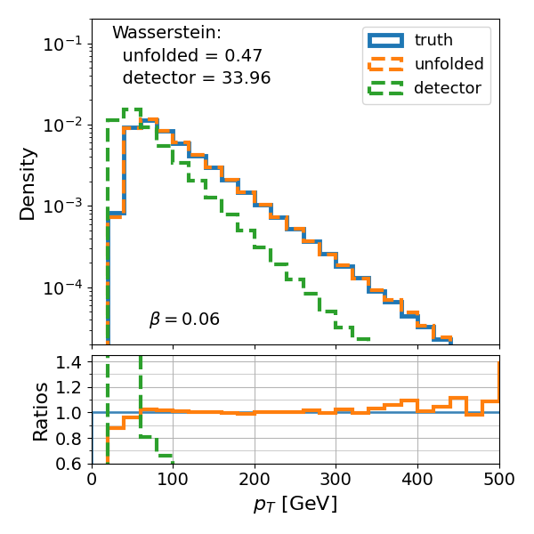
Figure 4: Unfolding results for three test datasets with different exponential $p_{T}$ distributions using a single cDDPM model. The model was trained on a combination of datasets with $\beta_{i}$ = 0.07, 0.3, and 0.7, and conditioned on the moments of the $p_{T}$ distributions. The cDDPM successfully unfolds the test datasets with $\beta_{j}$ = 0.06 (extrapolation), 0.2, and 0.5 (interpolation).

5.2 Physics Results

We test our approach on particle physics data by applying it to jet datasets from various processes sampled using the PYTHIA event generator (details of these synthetic datasets can be found in appendix B). The generated truth-level jets were passed through two different detector simulation frameworks to simulate particle interactions within an LHC detector. The detector simulations used were DELPHES with the standard CMS configuration, and another detector simulator developed using an analytical data-driven approximation for the $p_{T}$, $\eta$, and $\phi$ resolutions from results published by the ATLAS collaboration (more details in appendix C). The DELPHES CMS detector simulation is the standard and allows comparison to other machine-learning based unfolding algorithms, while the data-driven detector simulation tests the unfolding success under more drastic detector smearing.

In this setup, each jet is represented by a vector that includes the observables $[p_{T},\eta,\phi,E,p_{x},p_{y},p_{z}]$ both at truth-level ($\vec{x}$) and at detector level ($\vec{y}$). Following the approach described in section 4.2, the moments of the $p_{T}$ distributions are calculated per physics process and appended as part of the data vectors. A training dataset $\{\vec{x}^{\,m},\vec{y}^{\,m}\}_{\text{train}}=\bigcup_{i}\{\vec{x}^{\,m},\vec{y}^{\,m}\}_{i}$ was created for each detector configuration using simulated data from multiple physics processes $i$, which include $t\bar{t}$, $W$+jets, $Z$+jets, dijet, and leptoquark. Each process was simulated under a few different generator settings, such as varying parton distribution functions (PDFs), parton shower models, and with phase space biases.

A cDDPM was trained for each detector simulation and then used to unfold detector data from a variety of physics simulations. The test datasets were sampled both from processes that were included the training datasets ($\{\vec{x}^{\,m},\vec{y}^{\,m}\}_{i}$) and from processes that were purposefully left out of the training ($\{\vec{x}^{\,m},\vec{y}^{\,m}\}_{j}$). Unfolding results for the DELPHES CMS detector simulation can be seen in fig. 5, and results for the data-driven detector simulation in fig. 6. Additionally, the model was tested by unfolding datasets of combined processes meant to mimic a detector data distribution prior to background subtraction (fig. 7). A complete set of our physics results and additional tests can be found in appendix E.

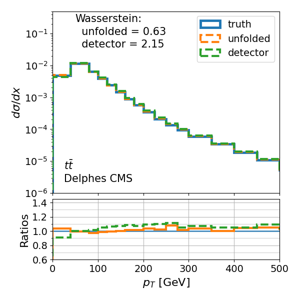
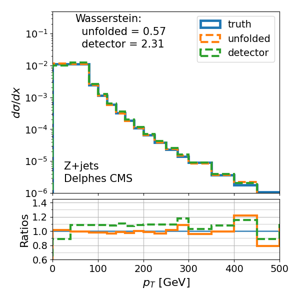
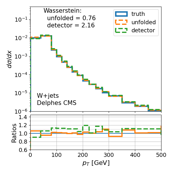
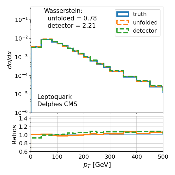
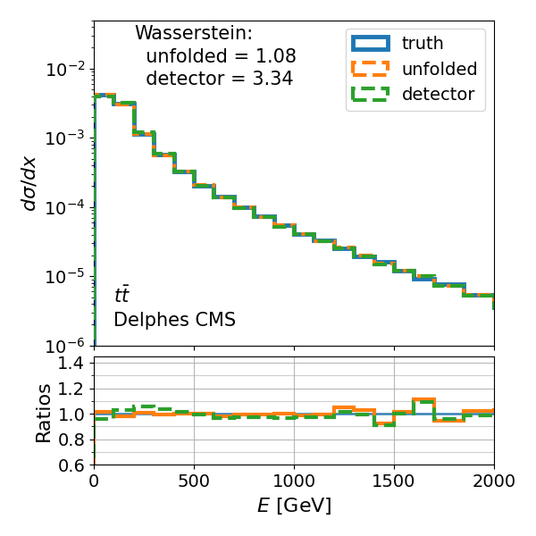
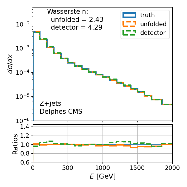
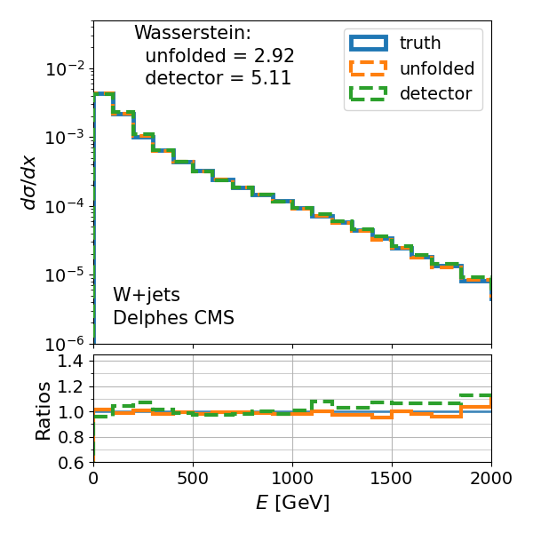
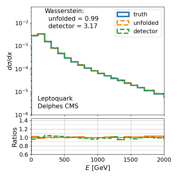
Figure 5: Unfolding performance of a single cDDPM on various simulated physics processes with detector effects simulated using DELPHES CMS. The training dataset included $t\bar{t}$, $Z$+jets, and $W$+jets processes, while the Leptoquark process was purposefully excluded. The cDDPM successfully unfolds the detector-level distributions, demonstrating its ability to generalize to new physics processes.

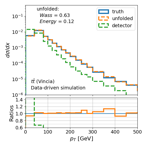
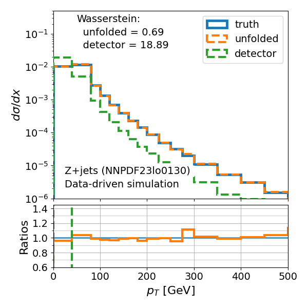
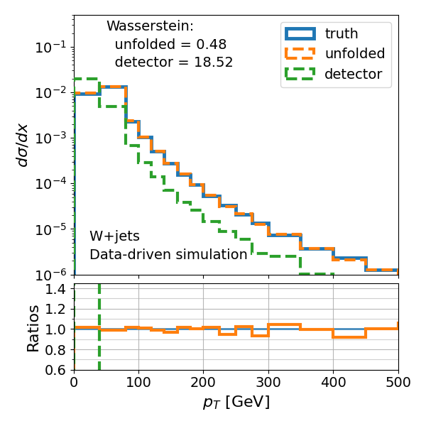
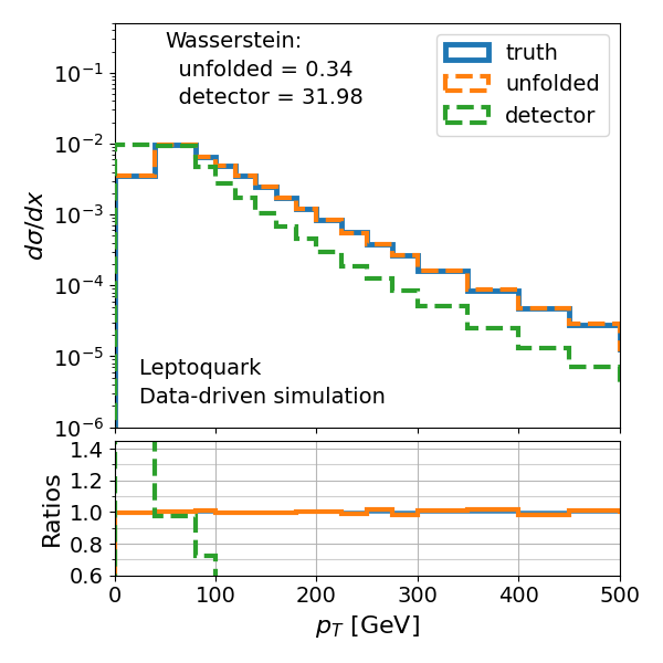
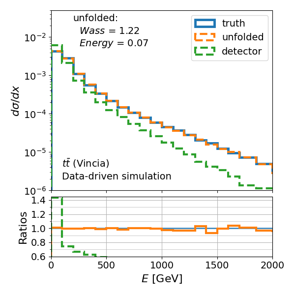
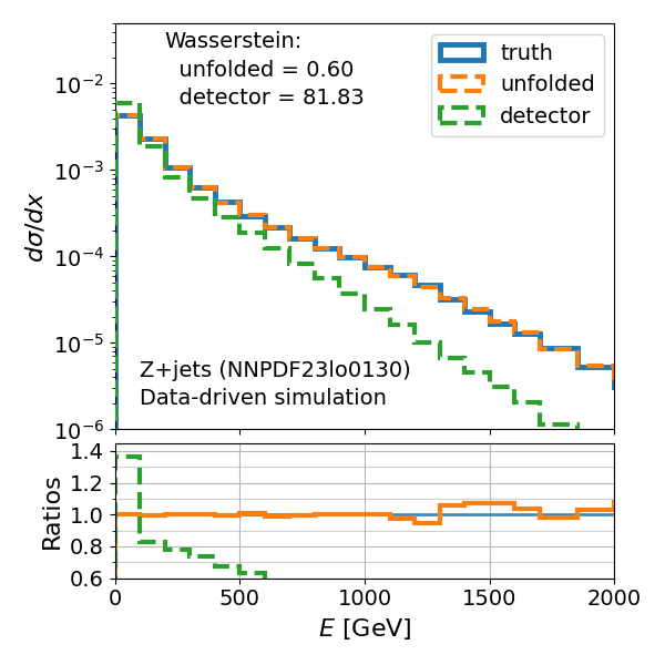
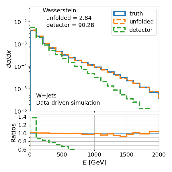
Figure 6: Unfolding results for various simulated physics processes using a single cDDPM, with detector effects simulated using an analytical data-driven approach. The $W$+jets process was included in the training dataset (along with others), while $t\bar{t}$, $Z$+jets, and Leptoquark processes were not. Despite the more drastic detector smearing, the cDDPM achieves significant improvement in unfolding the unseen processes compared to the detector-level distributions.

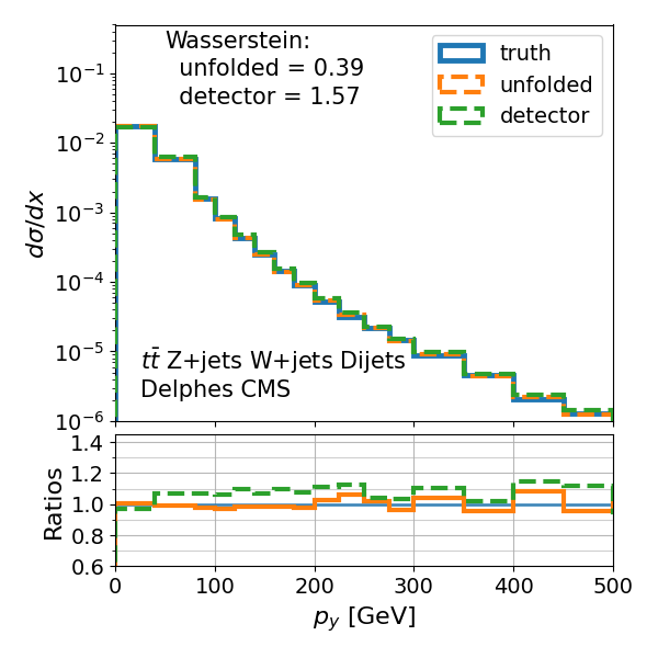
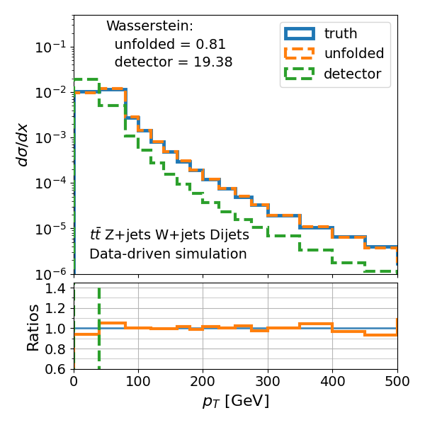
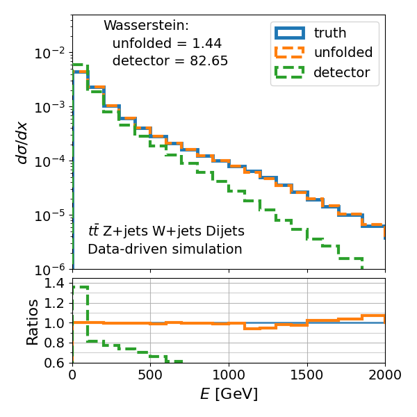
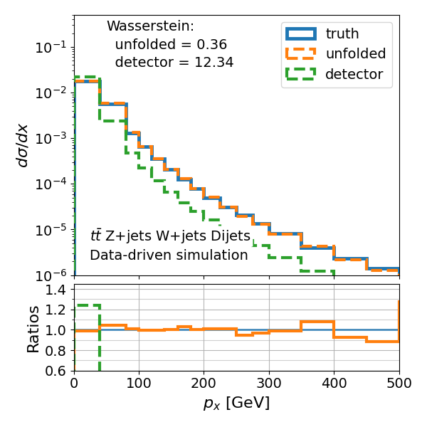
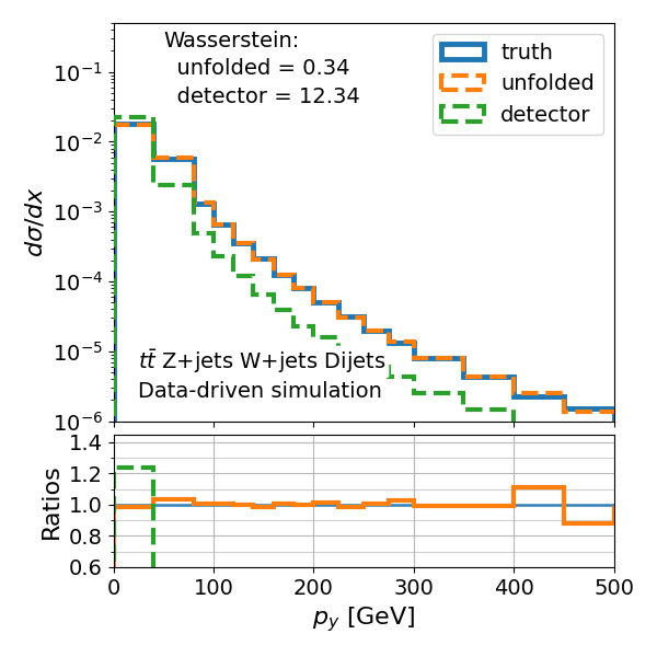
Figure 7: Unfolding performance of the cDDPM on combined datasets mimicking detector data prior to background subtraction. The top row shows results for the DELPHES CMS detector simulation, while the bottom row presents results for the data-driven detector simulation. The cDDPM successfully unfolds the combined datasets, demonstrating its potential for unfolding detector data before background subtraction.

6 Discussion

Our results demonstrate that a single cDDPM can successfully unfold detector effects on particle jets from a variety of physics processes, including those not seen during training. The distinguishing feature of our method is its non-iterative and flexible posterior sampling approach, which exhibits a strong inductive bias that allows the cDDPM to generalize to unseen processes without explicitly assuming the underlying physics distribution, setting it apart from other unfolding techniques so far.

The cDDPM’s ability to unfold data from combined processes presents a new opportunity to handle detector data prior to background subtraction, streamlining the unfolding process. These results are consistent for both the DELPHES CMS and the analytical data-driven detector simulations, indicating that the cDDPM’s performance is not drastically limited by the degree of detector smearing. We expect this approach to be applicable to other particles, detector-level observables, and event-wise quantities, enabling the reconstruction of full events after unfolding.

Several open questions remain regarding the implementation of the conditioning on the moments. These include optimal selection of priors and the number of moments required for the best unfolding performance. Further investigation is needed to determine the extent of the cDDPM’s inductive bias and its tolerance to variations in the underlying physics processes. Understanding these aspects will be crucial for refining the method and ensuring its robustness across a wide range of scenarios.

While this approach shows promise, improvements such as uncertainty estimation, accounting for systematic and experimental uncertainties, and handling particles falling outside detector thresholds are necessary to fully realize its potential. Incorporating these enhancements will be essential for making the cDDPM a reliable and comprehensive unfolding tool in high-energy physics. We leave these developments for future work.

Appendices

Appendix A Conditional DDPM Loss Derivation

In the proposed conditional DDPM, the forward process is a Markov chain that gradually adds Gaussian noise to the data according to a variance schedule $\beta$.

$$q(x_{t}|x_{t-1}):=\mathcal{N}(x_{t}\,;\sqrt{1-\beta_{t}}\,x_{t}\;,\;\beta_{t}\,\mathbf{I})$$

The reverse process is the joint distribution $p_{\theta}\,(x_{0:T}|y)=p_{\theta}\,(x_{0},x_{1},...x_{T}|y)$, and it is defined as a Markov chain with learned Gaussian transitions starting at $p(x_{T}|y)=\mathcal{N}(x_{T};0,\mathbb{I})$

$$p_{\theta}\,(x_{0:T}|y):=p(x_{T}|y)\prod^{T}_{t=1}p_{\theta}\,(x_{t-1}|x_{t}\,,y)$$

$$p_{\theta}(x_{t-1}|x_{t}\,,y):=\mathcal{N}\bigl{(}x_{t-1}\,;\mu_{\theta}(x_{t},t,y)\;,\;\Sigma_{\theta}(x_{t},t,y)\bigr{)}$$

Training is performed by optimizing the variational bound on negative log likelihood:

$$\begin{split}\mathbb{E}\bigl{[}-log\,p_{\theta}\,(x_{0}|y)\bigr{]}&\leq\mathbb{E}_{q}\left[-log\,\frac{p_{\theta}(x_{0:T}|y)}{q(x_{1:T}|x_{0})}\right]\\ &=\mathbb{E}_{q}\left[-log\,p(x_{T}|y)\>-\sum_{t\geq 1}log\,\frac{p_{\theta}(x_{t-1}|x_{t},y)}{q(x_{t}|x_{t-1})}\right]\;:=L\end{split}$$

Following the similar derivation provided in [13], this loss can then be rewritten using the KL-divergence

$$\begin{split}L&=\mathbb{E}_{q}\left[-log\frac{p_{\theta}(x_{0:T}|y)}{q(x_{1:T}|x_{0})}\right]\\ &=\mathbb{E}_{q}\left[-log\,p(x_{T}|y)\>-\sum_{t\geq 1}log\,\frac{p_{\theta}(x_{t-1}|x_{t},y)}{q(x_{t}|x_{t-1})}\right]\\ &=\mathbb{E}_{q}\left[-log\,p(x_{T}|y)\>-\sum_{t>1}log\,\frac{p_{\theta}(x_{t-1}|x_{t},y)}{q(x_{t}|x_{t-1})}\>-log\,\frac{p_{\theta}(x_{0}|x_{1},y)}{q(x_{1}|x_{0})}\right]\\ &=\mathbb{E}_{q}\left[-log\,p(x_{T}|y)\>-\sum_{t>1}log\,\frac{p_{\theta}(x_{t-1}|x_{t},y)}{q(x_{t-1}|x_{t},x_{0})}\cdot\frac{q(x_{t-1}|x_{0})}{q(x_{t}|x_{0})}\>-log\,\frac{p_{\theta}(x_{0}|x_{1},y)}{q(x_{1}|x_{0})}\right]\\ &=\mathbb{E}_{q}\left[-log\,\frac{p(x_{T}|y)}{q(x_{T}|x_{0})}\>-\sum_{t>1}log\,\frac{p_{\theta}(x_{t-1}|x_{t},y)}{q(x_{t-1}|x_{t},x_{0})}\>-log\,p_{\theta}(x_{0}|x_{1},y)\right]\\ &=\mathbb{E}_{q}\left[\underbrace{D_{KL}\bigl{(}q(x_{T}|x_{0})\parallel p(x_{T}|y)\bigr{)}}_{L_{T}}+\sum_{t>1}\underbrace{D_{KL}\bigl{(}q(x_{t-1}|x_{t},x_{0})\parallel p_{\theta}(x_{t-1}|x_{t},y)\bigr{)}}_{L_{1:T-1}}-\underbrace{\log p_{\theta}(x_{0}|x_{1},y)}_{L_{0}}\right]\\ \end{split}$$

The term $L_{T}$ is a constant, as it is the KL-divergence between two distributions of pure noise, and the $L_{0}$ term is a final denoising step with no comparison to the forward process posteriors. For the term $L_{1:T-1}$, the forward process posteriors can be written as

$$q(x_{t+1}|x_{t},x_{0})=\mathcal{N}(x_{t+1};\tilde{\mu}_{t}(x_{t},x_{0}),\tilde{\beta}_{t}I)$$

$$\text{where}~{}\tilde{\mu}_{t}(x_{t},x_{0})=\left(\frac{\beta_{t}\sqrt{\bar{\alpha}_{t-1}}}{1-\bar{\alpha}_{t}}x_{0}+\frac{\sqrt{\bar{\alpha}_{t}}(1-\bar{\alpha}_{t-1})}{(1-\bar{\alpha}_{t})}x_{t}\right)~{}\text{and}~{}\tilde{\beta}_{t}=\frac{1-\bar{\alpha}_{t-1}}{1-\bar{\alpha}_{t}}\beta_{t}$$

and the reverse process posterior as

$$p_{\theta}(x_{t-1}|x_{t}\,,y)=\mathcal{N}(x_{t-1}\,;\mu_{\theta}(x_{t},t,y)\;,\;\Sigma_{\theta}(x_{t},t,y))$$

$$\text{where}~{}\Sigma_{\theta}(x_{t},t,y)=\sigma^{2}\mathbf{I},\sigma^{2}=\beta_{t}\text{ or }\sigma^{2}=\tilde{\beta}_{t}$$

and a parametrization for $\mu_{\theta}(x_{t},t,y)$ such that it predicts $\tilde{\mu}_{t}(x_{t},x_{0})$. With this the loss becomes

$$L_{t-1}=\mathbb{E}\left[\frac{1}{2\sigma_{t}^{2}}\parallel\tilde{\mu}_{t}\,(x_{t},x_{0})-\mu_{\theta}\,(x_{t},t,y)\parallel^{2}\right]+C$$

where $C$ is a constant, and $\tilde{\mu}_{t}$ and $\mu_{\theta}$ can be reparametrized using $x_{t}=\sqrt{\bar{\alpha_{t}}}\,x_{0}+\sqrt{1-\bar{\alpha_{t}}}\,\epsilon$ and reduced to

$$L_{t-1}=\mathbb{E}_{\epsilon,x_{0},y}\left[\frac{\beta_{t}^{2}}{2\sigma_{t}^{2}\alpha_{t}(1-\bar{\alpha}_{t})}\parallel\epsilon-\epsilon_{\theta}\,(\sqrt{\bar{\alpha}_{t}}x_{0}+\sqrt{1-\bar{\alpha}_{t}}\epsilon,t,y)\parallel^{2}\right].$$

Finally we can write a simplified version of the loss with the terms differentiable in $\theta$ as

$$\begin{split}L_{simple}(\theta)&=\mathbb{E}_{\epsilon,x_{t},y}\left[\parallel\epsilon-\epsilon_{\theta}\,(\sqrt{\bar{\alpha}_{t}}x_{0}+\sqrt{1-\bar{\alpha}_{t}}\epsilon,t,y)\parallel^{2}\right]\\ &=\mathbb{E}_{\epsilon,x_{t},y}\left[\parallel\epsilon-\epsilon_{\theta}\,(x_{t},t,y)\parallel^{2}\right].\end{split}$$

Appendix B Physics Simulations

Physics datasets were generated using PYTHIA 8.3 Monte-Carlo event generator. The simulations were run for proton-proton collisions at a center-of-mass energy of 13 TeV to emulate LHC physics interactions. The various physics processes used in this study were chosen for their high jet-production cross-section across a large jet energy range. The chosen processes were hadronic decays of $t\bar{t}$, $(Z\rightarrow\mu\bar{\mu})+$jets, $(W\rightarrow\mu\bar{\nu})+$jets, dijets, and the new-physics process of leptoquarks. Each of these processes were run under multiple generator settings, with varying parton distribution functions (PDFs), parton shower models, and with an imposed phase space bias that increased the probability of generating events with high jet energies. For simulations where a phase space bias was applied, the events are sampled in the phase space as $(\hat{p}_{T}/p_{T}^{\text{ref}})^{a}$, where we set $p_{T}^{\text{ref}}=100$ GeV and $a=5$ such that events with a $p_{T}$ over 100 GeV will be oversampled, increasing the event statistics in high-energy regions [3]. A list of the physics processes generated for the DELPHES CMS detector simulation is shown in table 1, and those generated for the data-driven detector simulation in table 2. Unless stated otherwise, the simulations were run with the PYTHIA simple parton shower model and no phase space bias.

Process	PDF (Phase Space Bias)	In Training?
$t\bar{t}$	CTEQ6L1	✓
	CTEQ6L1 (biased)	✓
$Z+$jets	CTEQ6L1	✓
	CTEQ6L1 (biased)	✓
$W+$jets	CTEQ6L1
Dijets	CTEQ6L1	✓
	CTEQ6L1 (biased)	✓
Leptoquark	CTEQ6L1

Table 1: List of physics simulations generated for the DELPHES CMS detector simulation, along with the corresponding parton distribution functions (PDFs), phase space biases, and their inclusion in the training dataset.

Process	PDF with Parton Shower (Phase Space Bias)	In Training?
$t\bar{t}$	CT14lo	✓
	CT14lo (biased)	✓
	CT14lo with Vincia
	NNPDF23_lo_as_0130_qed	✓
	CTEQ6L1	✓
	CTEQ6L1 (biased)
$Z+$jets	CT14lo	✓
	CT14lo (biased)	✓
	NNPDF23_lo_as_0130_qed
	CTEQ6L1	✓
	CTEQ6L1 (biased)
$W+$jets	CT14lo	✓
	CT14lo (biased)	✓
	NNPDF23_lo_as_0130_qed
	CTEQ6L1
Dijets	CT14lo	✓
	NNPDF23_lo_as_0130_qed
	CTEQ6L1	✓
	CTEQ6L1 (biased)	✓
Leptoquark	CT14lo
	CT14lo (biased)
	NNPDF23_lo_as_0130_qed
	CTEQ6L1

Table 2: List of physics simulations generated for the data-driven detector simulation, along with the corresponding parton distribution functions (PDFs), parton shower models, phase space biases, and their inclusion in the training dataset. Simulations not included in the training dataset were used as test datasets.

Appendix C Detector Simulation and Jet Matching

Our results present the unfolding of detector effects from two different detector simulation frameworks: DELPHES and a data-driven approach. DELPHES is a framework developed for the simulation of multipurpose detectors for physics studies [12]. Specifically, the DELPHES CMS configuration is frequently used as the detector simulation of choice in recent machine-learning based unfolding studies.

To test the unfolding performance under more exaggerated detector effects, we developed a framework with a data-driven detector simulation using jet energy resolution results published by the ATLAS collaboration at a centre-of-mass energy of 8 TeV with an integrated luminosity of 20 $\text{fb}^{-1}$ [8]. In this framework, the PYTHIA event generator is used to simulate truth-level particles, and the resulting partons are grouped into jets using the FastJet package [6]. The transverse momentum $p_{T}$, azimuthal angle $\phi$, and pseudorapidity $\eta$ of each truth-level jet is then smeared following the ATLAS calibration and resolution functions. For the $\phi$ and $\eta$ smearing, the effect is small since the angular resolution effects are proportional to the detector granularity. We assume that there is no angular shift and apply a smearing to $\phi$ and $\eta$ by sampling from a Gaussian centered at the truth-level value and with a $\sigma$ equal to the detector resolution for the particle. We apply a quadratic fit ($\sigma=a\,p_{T}^{~{}2}+b\,p_{T}+c$) to the calibration data presented in [8] to approximate the detector resolution in $\phi$ ($a=5.6\times 10^{-8}$, $b=-1.12\times 10^{-4}$, $c=0.06$) and $\eta$ ($a=8.4\times 10^{-8}$, $b=1.68\times 10^{-4}$, $c=0.09$).

In principle, a calorimeter cell measurement is an energy measurement, but since the jet calibration studies precisely measure the jet $p_{T}$ resolution, we apply a shift and a smearing to the jet $p_{T}$ instead. The jet $p_{T}$ resolution can be expressed as $\sigma_{p_{T}}=p_{T}\sqrt{\frac{a}{p_{T}^{~{}2}}+\frac{b}{p_{T}}+c}$ and a fit of this function is applied to the jet calibration data (specifically for jets with $0<|\eta\,|<0.8$ for simplicity) to approximate this resolution ($a=11.09$, $b=0.504$, $c=0.0009$). The jet $p_{T}$ also has a calibration shift, which can be defined from the data as $p_{T}\,^{\prime}=p_{T}\left(0.0063\sqrt{p_{T}-20}+0.6\right)$. The detector smeared $p_{T}$ is then defined by sampling from a Gaussian centered at $p_{T}\,^{\prime}$ and with $\sigma$ equal to the jet $p_{T}$ resolution. Finally, the smeared energy for each jet is calculated with $E=\sqrt{m^{2}+|\vec{p}\,|^{2}}$ by fixing the mass of the particle $m$ and using the smeared $p_{T}$. Pseudocode of this smearing procedure is shown fig. 8 in for clarity.

Algorithm 3 Data-Driven Detector Smearing

Input: truth-level dataset with [$p_{T}^{\>\text{true}}$, $\eta^{\text{true}}$, $\phi^{\text{true}}$, $m^{\text{true}}$] per jet

For each jet in the dataset do

1. $\sigma_{\eta}\leftarrow 0.000000084\,(p_{T}^{\>\text{true}})^{2}-0.000168\,p_{T}^{\>\text{true}}+0.09$

2. $\sigma_{\phi}\leftarrow 0.000000056\,(p_{T}^{\>\text{true}})^{2}-0.000112\,p_{T}^{\>\text{true}}+0.06$

3. $\sigma_{p_{T}}\leftarrow p_{T}^{\>\text{true}}\sqrt{\frac{11.09}{(p_{T}^{\>\text{true}})^{2}}+\frac{0.504}{p_{T}^{\>\text{true}}}+0.6}$

4. $\eta^{\text{det}}\leftarrow\mathcal{N}(\eta^{\text{true}},\sigma_{\eta})$

5. $\phi^{\text{det}}\leftarrow\mathcal{N}(\phi^{\text{true}},\sigma_{\phi})$

6. $p_{T}^{\,\text{shift}}\leftarrow p_{T}^{\>\text{true}}\left(0.0063\sqrt{p_{T}^{\>\text{true}}-20}+0.6\right)$

7. $p_{T}^{\>\text{det}}\leftarrow\mathcal{N}(p_{T}^{\,\text{shift}},\sigma_{p_{T}})$

8. $E^{\text{det}}\leftarrow\sqrt{\left((p_{T}^{\>\text{det}}\,cosh(\eta^{\text{det}})\right)^{2}+(m^{\text{true}})^{2}}$

Return detector-level dataset with [$p_{T}^{\>\text{det}}$, $\eta^{\text{det}}$, $\phi^{\text{det}}$, $E^{\text{det}}$] per jet

Figure 8: Pseudocode for the data-driven detector smearing algorithm. The algorithm takes a truth-level dataset with [$p_{T}^{true}$, $\eta^{true}$, $\phi^{true}$, $m^{true}$] per jet and applies smearing to each observable based on the detector resolution functions derived from ATLAS calibration data. The smeared observables [$p_{T}^{det}$, $\eta^{det}$, $\phi^{det}$, $m^{det}$] are returned for each jet in the detector-level dataset.

In Monte Carlo based detector simulation methods used by LHC experiments (like Geant4), the detector smearing occurs at the parton level instead of at the jet level as we defined here. As a result, the jet-clustering algorithm is applied independently to the truth-level data and the detector-level data and it is necessary to implement a jet-matching algorithm to identify which detector-level jet pertain to which truth-level jet within an event. To mimic any confounding effects that might result from mismatched jets in those simulations, we also implement jet-matching in our data-driven detector simulation. After detector smearing, the jets within an event are reordered by decreasing $p_{T}$ such that we lose track of which detector-level jet came from each truth-level jet. The angular distance $\Delta R=\sqrt{(\Delta\phi)^{2}+(\Delta\eta)^{2}}$, where $\Delta\phi=\phi^{\text{det}}-\phi^{\text{true}}$ and $\Delta\eta=\eta^{\text{det}}-\eta^{\text{true}}$, is calculated between each truth-level and detector-level jet in an event, and the pairs with the lowest $\Delta R$ are matched, up to a maximum value set to $\Delta R=0.4$. This maximum limit is defined by the maximum radius limit in the definition of a jet.

Appendix D Toy Model Results

The full unfolding results of the toy model tests are shown here, including the $\eta$, $\phi$, and $E$ distributions of the data 4-vectors. In fig. 9 we show the full results of multidimensional unfolding tests as well as the tests on the cDDPM dependence on the training prior when learning the posterior. In fig. 10 the full results for the moments-based unfolding are shown.

In fig. 10 we show the complete 4-vector unfolding results that demonstrate the cDDPM’s capacity to learn the posterior distribution $P(\mathbf{x}|\mathbf{y})$ given a dataset of pairs ${\vec{x},\vec{y}}$, as evidenced by the close match between the unfolded and truth-level distributions for all particle properties. Moreover, the bottom row of fig. 10 highlights the cDDPM’s robustness to changes in the marginal distributions of the training dataset.

In fig. 10 we present the complete unfolding results for the multidimensional toy model tests using a class of exponential functions. The successful unfolding of all particle properties for the test datasets underscores the cDDPM’s capacity to generalize beyond the specific distributions seen during training.

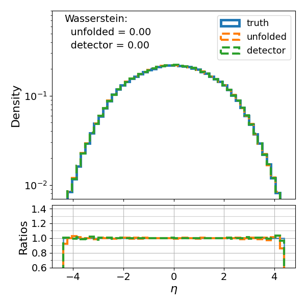
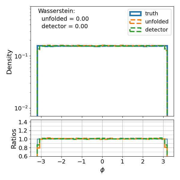
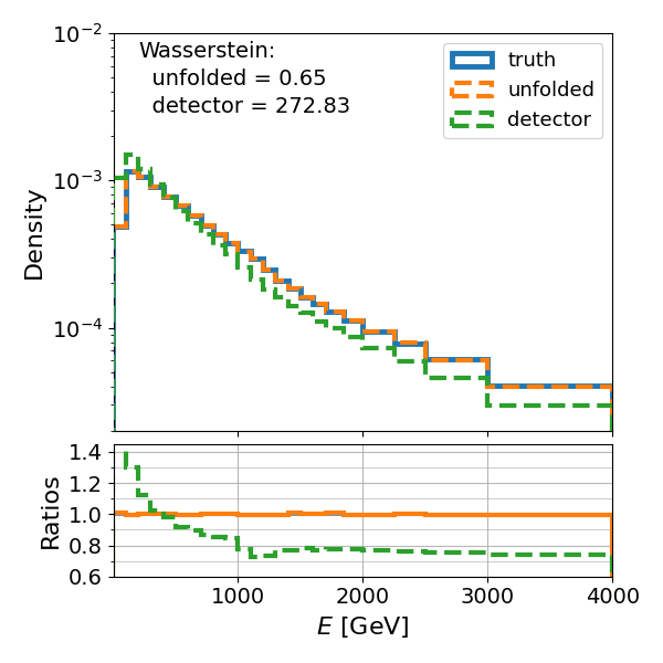
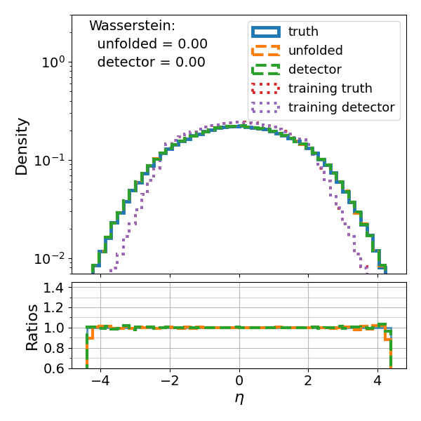
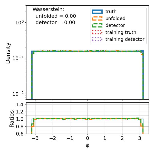
Figure 9: Complete unfolding results for the multidimensional toy model tests, demonstrating the cDDPM’s ability to learn the posterior $P(x|y)$ given a dataset of pairs $\{x,y\}$. The bottom row shows the unfolding performance when the cDDPM is trained on an alternative dataset with different marginal distributions but the same posterior, confirming that the cDDPM’s sampling is based on the learned posterior without significant dependence on the training prior.

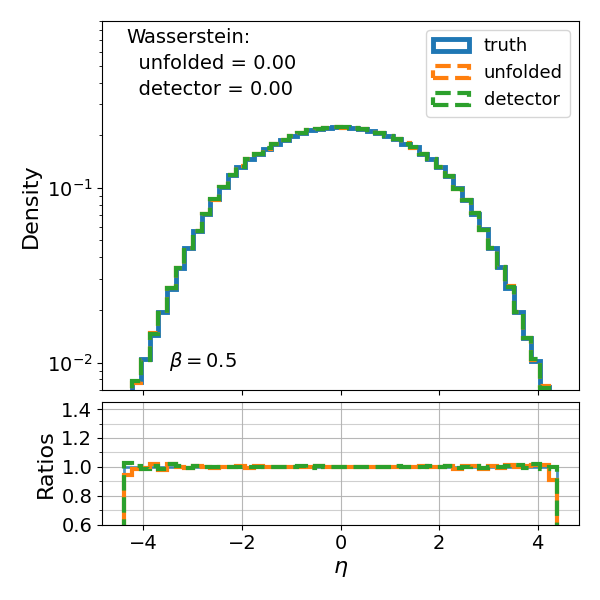
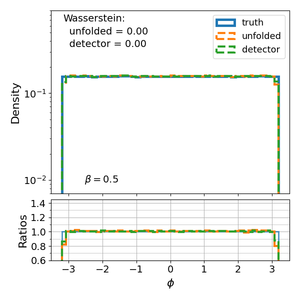
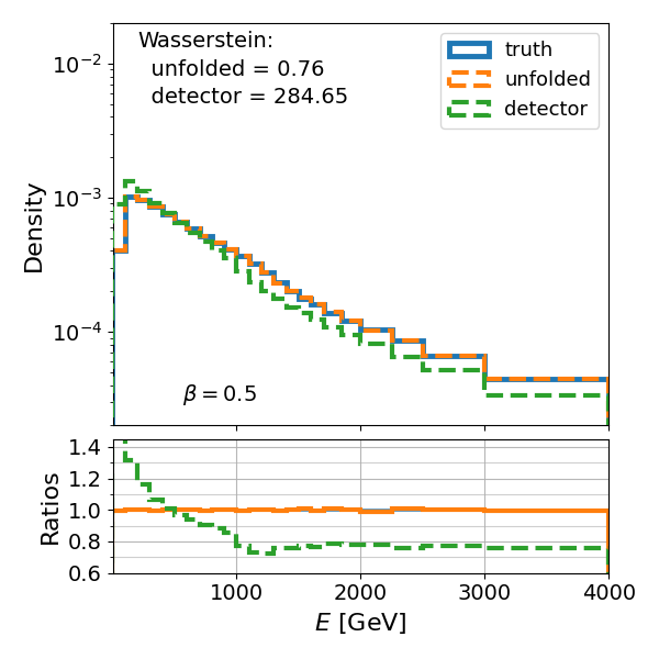
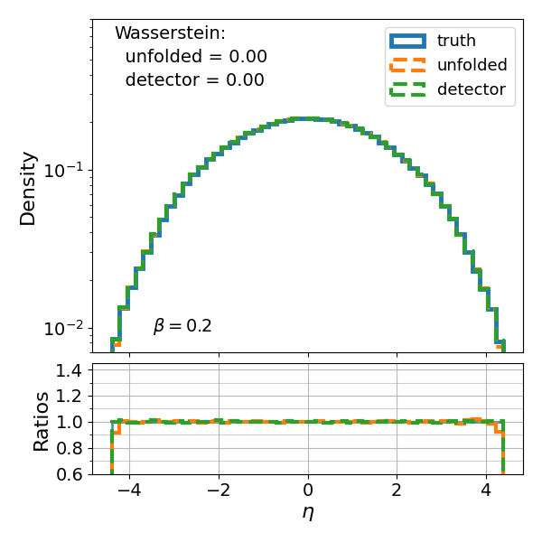
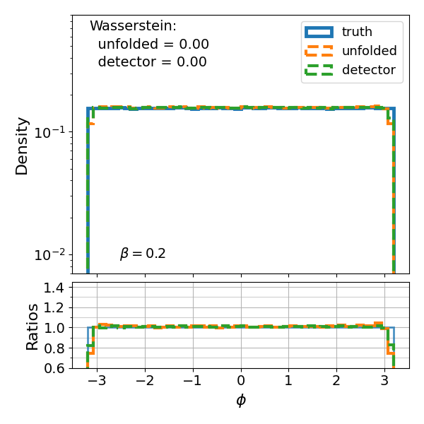
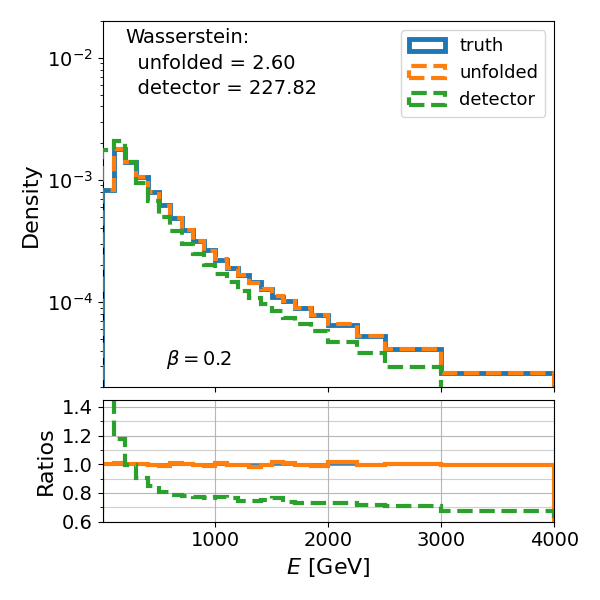
Figure 10: Complete unfolding results for the multidimensional toy model tests using a class of exponential functions. The cDDPM is trained on datasets with different exponential distributions (characterized by $\beta_{i}$) and conditioned on the moments of the $p_{T}$ distributions. The successful unfolding of the test datasets demonstrates the cDDPM’s ability to interpolate and extrapolate within the class of distributions based on the provided moments.

Appendix E Complete Physics Results

In fig. 11 and fig. 12 we present the unfolding results for the remaining particle properties ($\eta$, $\phi$, $E$, $p_{x}$, $p_{y}$, $p_{z}$) that were not shown in the main text. These additional plots demonstrate the cDDPM’s ability to successfully unfold the full particle vector, providing a comprehensive view of its performance across all dimensions.

The tables in this appendix (table 3 and table 4) provide a detailed breakdown of the unfolding performance metrics for each particle property and dataset. Furthermore, these metrics (Energy distance, Wasserstein distance between histograms, and KL divergence between histograms) offer a more in-depth perspective on the unfolding quality.

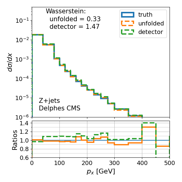
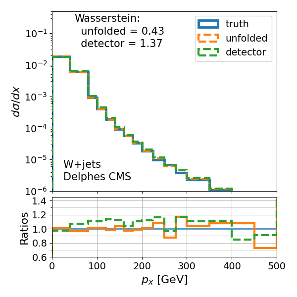
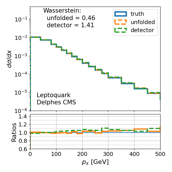
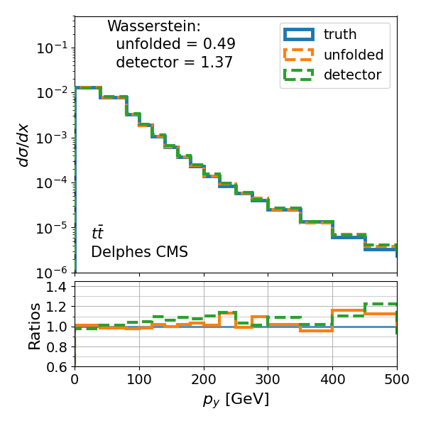
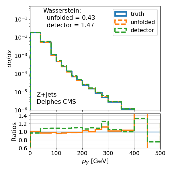
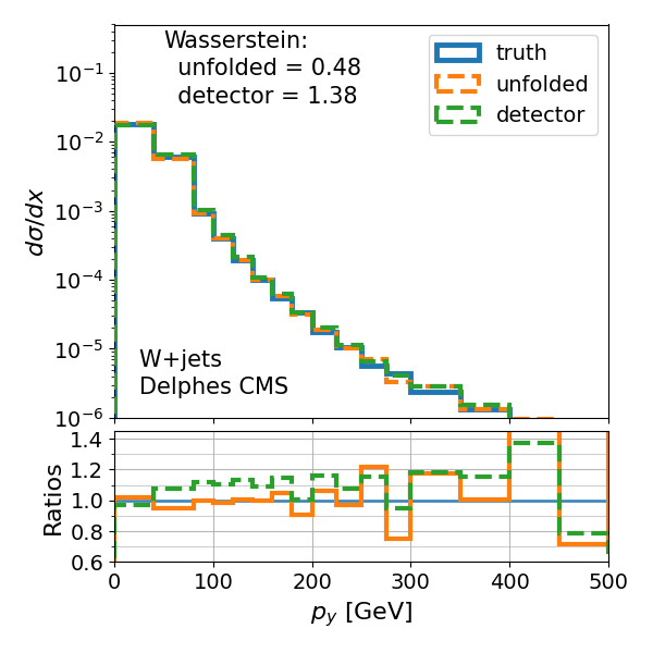
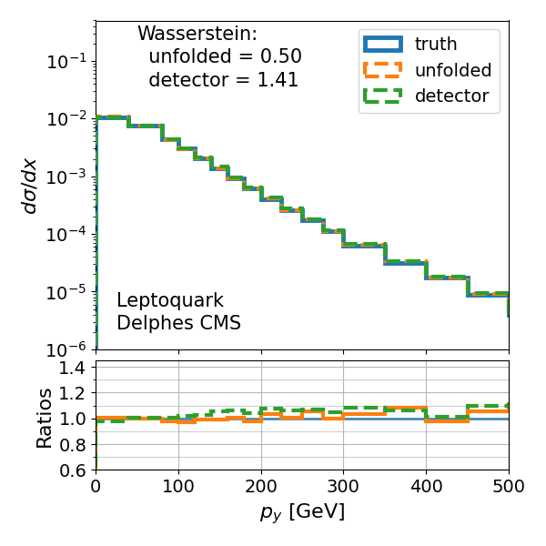
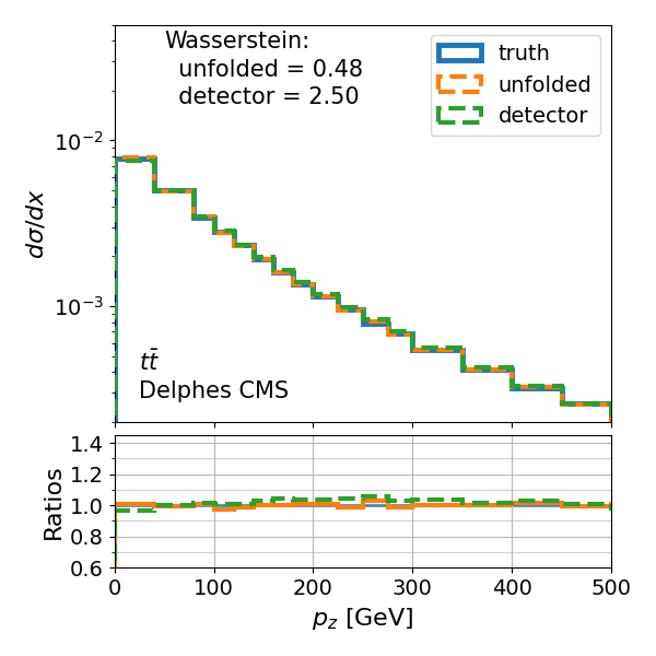
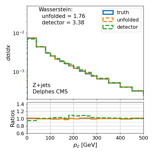
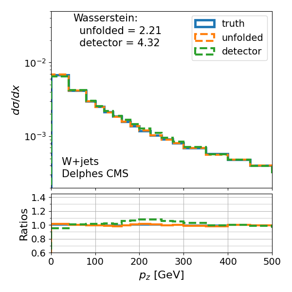
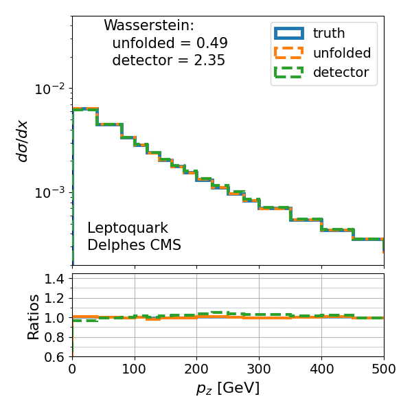
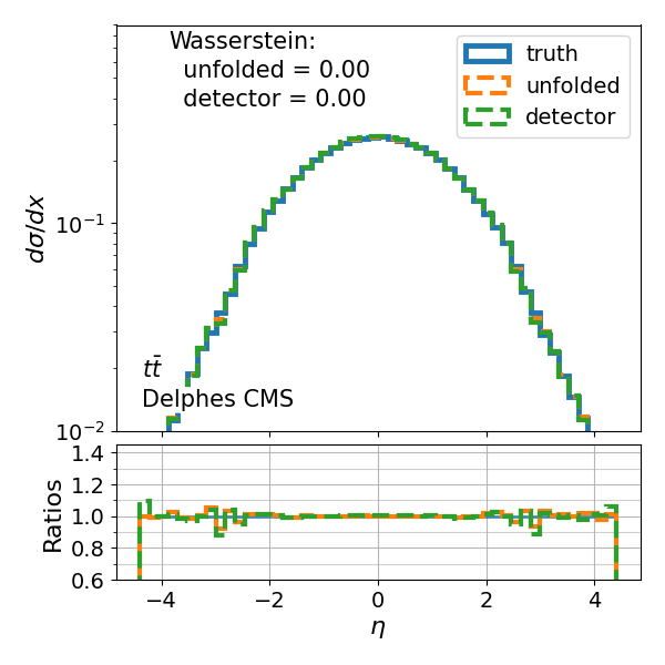
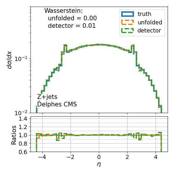
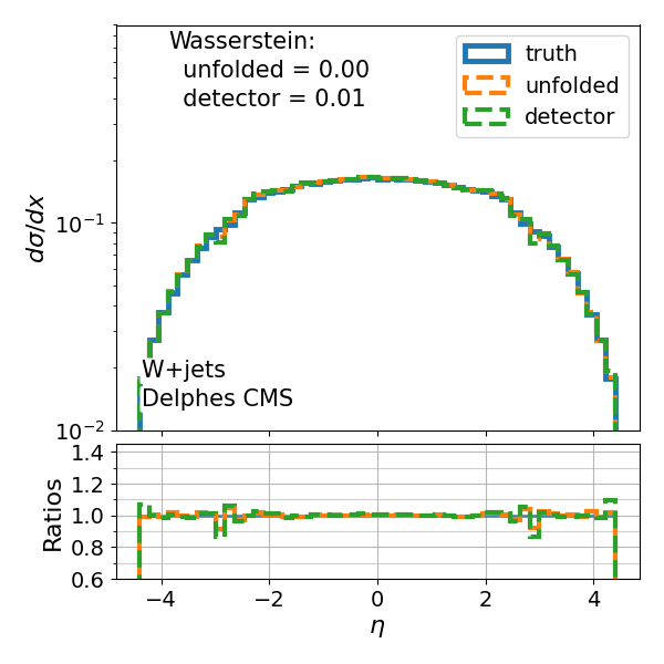
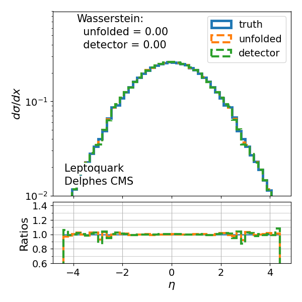
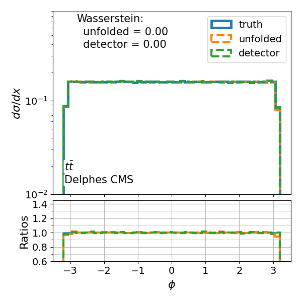
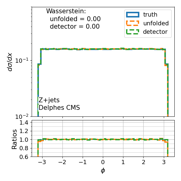
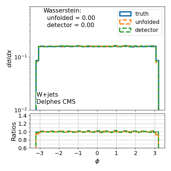
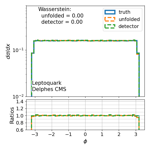
Figure 11: Unfolding performance of a single cDDPM on the remaining particle properties ($\eta$, $\phi$, $p_{x}$, $p_{y}$, $p_{z}$) for various simulated physics processes with detector effects simulated using DELPHES CMS. These plots show the particle vector properties that were not included in the main results in fig. 5.

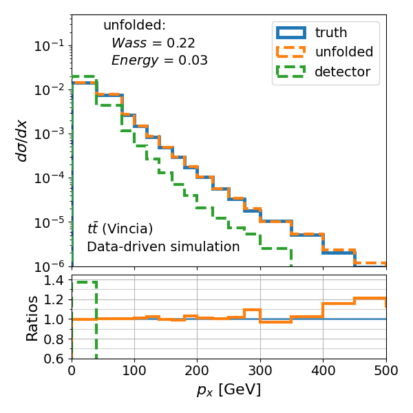
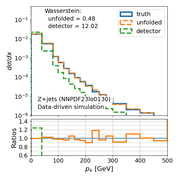
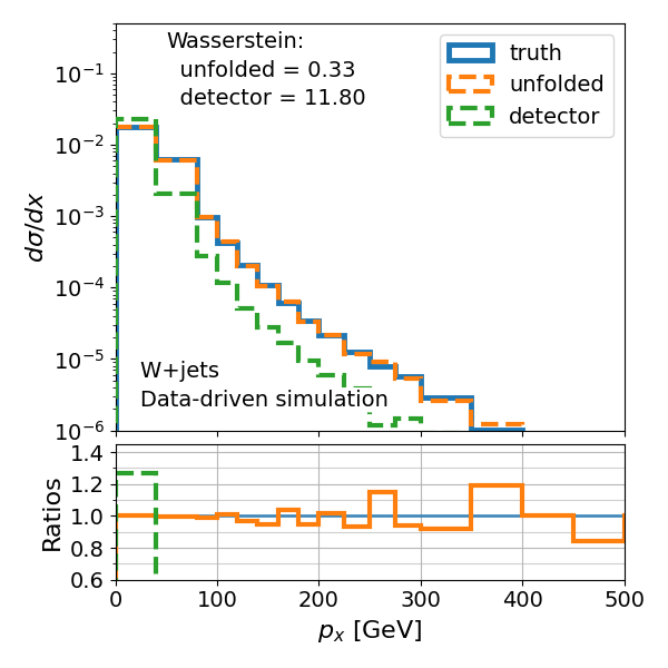
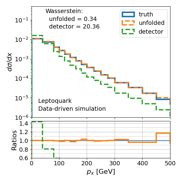
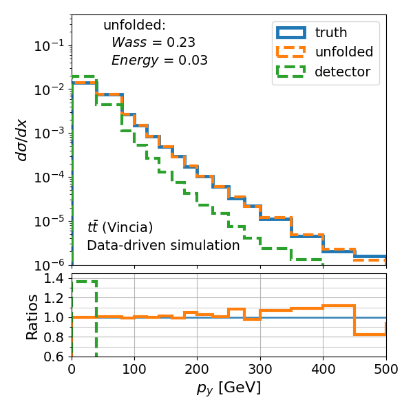
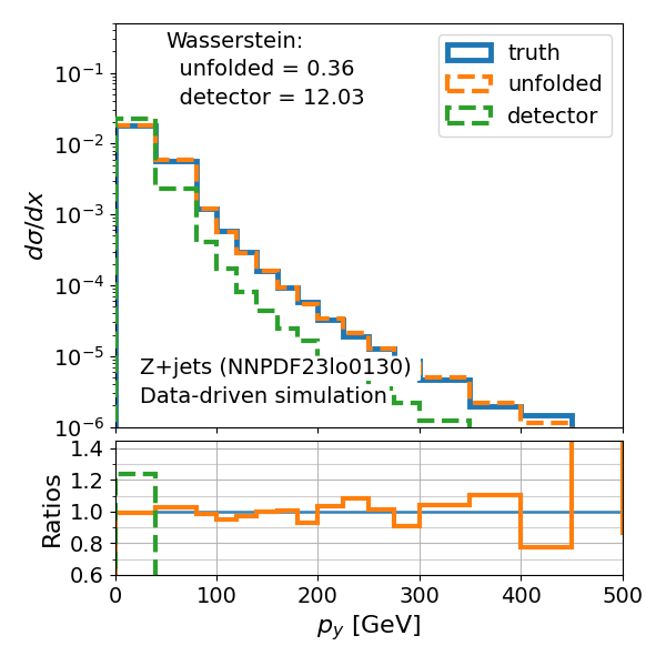
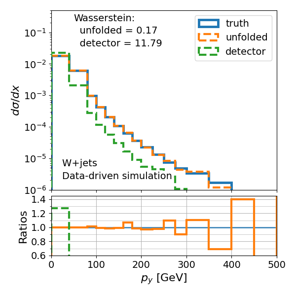
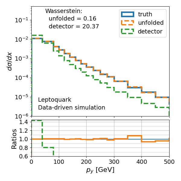
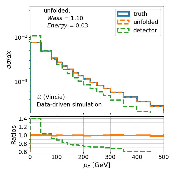
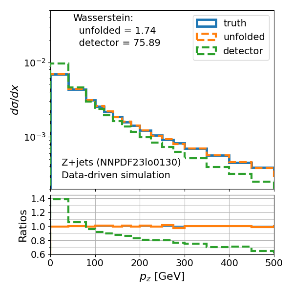
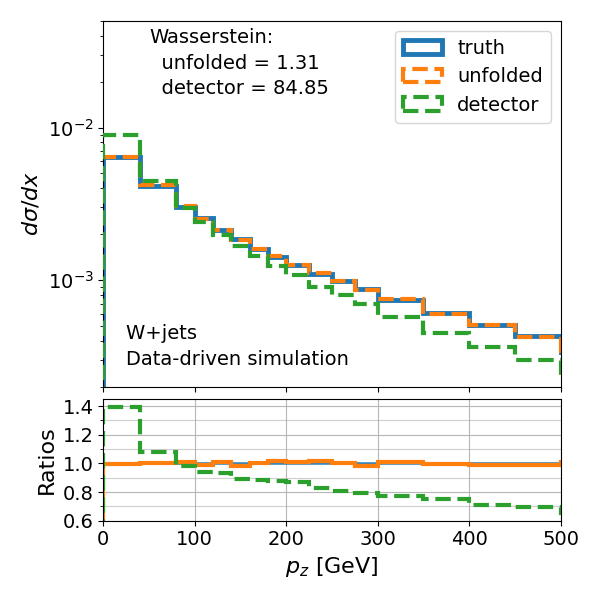
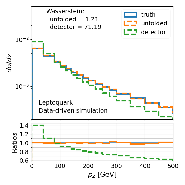
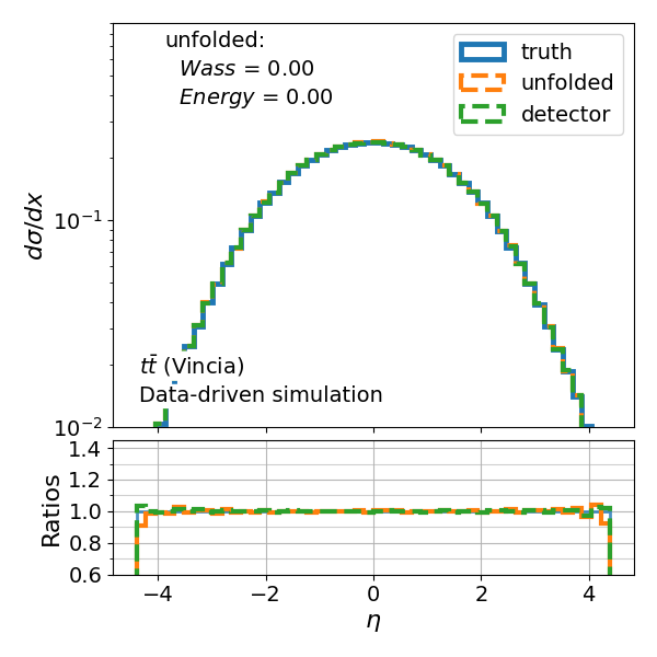
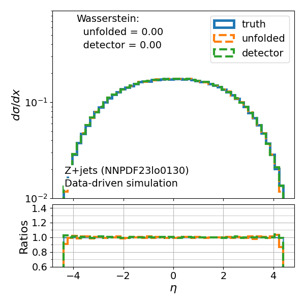
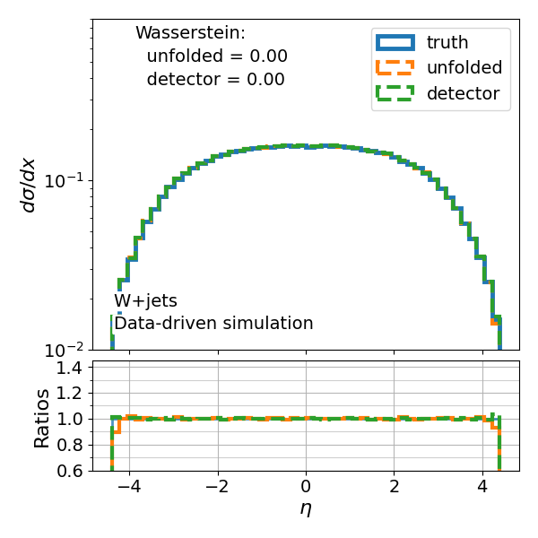
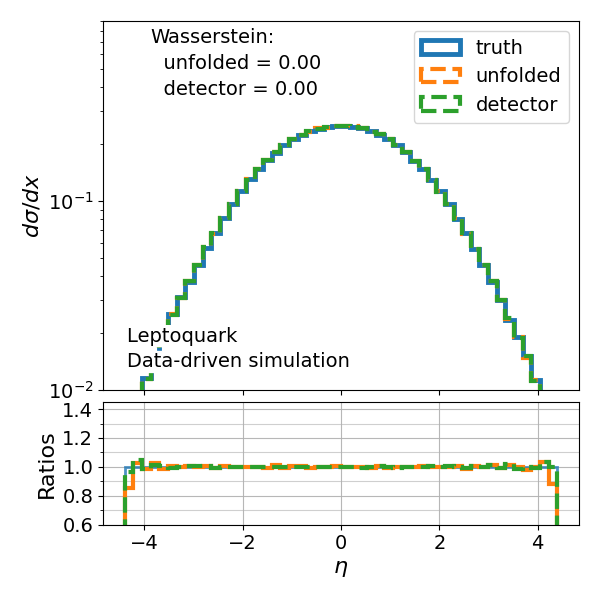
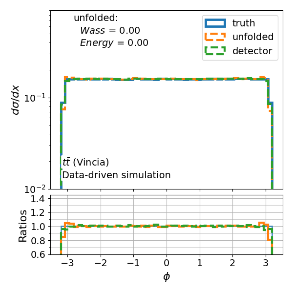
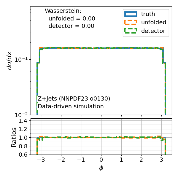
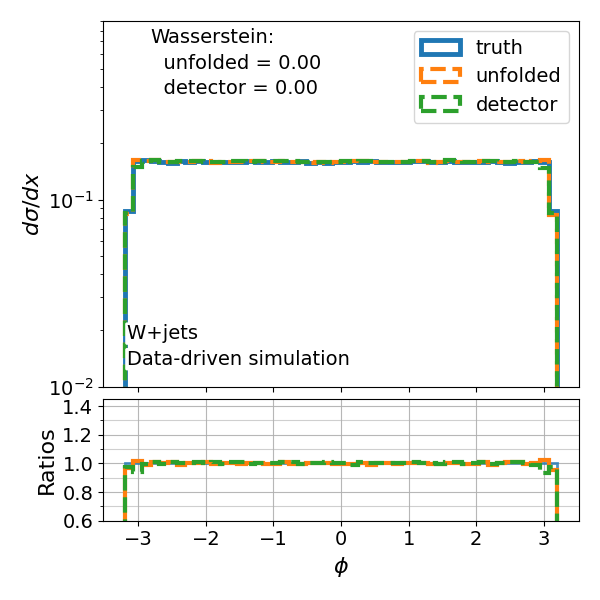
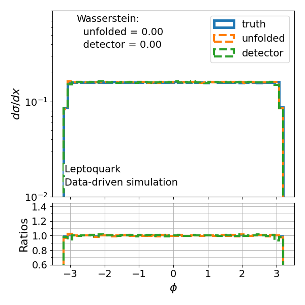
Figure 12: Unfolding performance of a single cDDPM on the remaining particle properties ($\eta$, $\phi$, $p_{x}$, $p_{y}$, $p_{z}$) for various simulated physics processes with detector effects simulated using an analystical data-driven approach. These plots show the particle vector properties that were not included in the main results in fig. 6.

			Sample		Histogram
			Wasserstein	Energy	Wasserstein	KL Divergence
$t\bar{t}$ (CTEQ6L1)	$p_{T}$	unfolded:	0.634	0.070	0.00003	0.00020
		detector:	2.150	0.249	0.00006	0.00125
	$\eta$	unfolded:	0.001	0.001	0.00073	0.00009
		detector:	0.004	0.002	0.00093	0.00017
	$\phi$	unfolded:	0.002	0.001	0.00037	0.00005
		detector:	0.001	0.001	0.00027	0.00002
	$E$	unfolded:	1.083	0.110	0.00001	0.00010
		detector:	3.339	0.253	0.00002	0.00068
	$p_{x}$	unfolded:	0.350	0.032	0.00001	0.00006
		detector:	1.371	0.117	0.00004	0.00064
	$p_{y}$	unfolded:	0.488	0.044	0.00002	0.00016
		detector:	1.373	0.117	0.00004	0.00064
	$p_{z}$	unfolded:	0.484	0.020	0.00002	0.00006
		detector:	2.503	0.114	0.00004	0.00035
Z+jets (CTEQ6L1)	$p_{T}$	unfolded:	0.569	0.104	0.00002	0.00009
		detector:	2.306	0.473	0.00013	0.00465
	$\eta$	unfolded:	0.002	0.001	0.00092	0.00016
		detector:	0.006	0.003	0.00164	0.00042
	$\phi$	unfolded:	0.002	0.001	0.00068	0.00007
		detector:	0.001	0.001	0.00081	0.00004
	$E$	unfolded:	2.430	0.143	0.00000	0.00008
		detector:	4.288	0.381	0.00002	0.00092
	$p_{x}$	unfolded:	0.334	0.046	0.00002	0.00011
		detector:	1.470	0.193	0.00006	0.00138
	$p_{y}$	unfolded:	0.428	0.063	0.00002	0.00020
		detector:	1.471	0.193	0.00006	0.00136
	$p_{z}$	unfolded:	1.757	0.052	0.00002	0.00008
		detector:	3.377	0.183	0.00006	0.00091
W+jets (CTEQ6L1)	$p_{T}$	unfolded:	0.758	0.169	0.00006	0.00118
		detector:	2.157	0.399	0.00011	0.00347
	$\eta$	unfolded:	0.002	0.001	0.00105	0.00019
		detector:	0.006	0.003	0.00147	0.00044
	$\phi$	unfolded:	0.002	0.001	0.00070	0.00009
		detector:	0.001	0.001	0.00087	0.00009
	$E$	unfolded:	2.916	0.172	0.00001	0.00010
		detector:	5.108	0.334	0.00002	0.00090
	$p_{x}$	unfolded:	0.430	0.066	0.00002	0.00018
		detector:	1.371	0.169	0.00006	0.00135
	$p_{y}$	unfolded:	0.480	0.076	0.00003	0.00021
		detector:	1.376	0.169	0.00006	0.00134
	$p_{z}$	unfolded:	2.213	0.071	0.00002	0.00007
		detector:	4.321	0.164	0.00005	0.00077
Leptoquark (CTEQ6L1)	$p_{T}$	unfolded:	0.778	0.070	0.00003	0.00014
		detector:	2.214	0.211	0.00004	0.00059
	$\eta$	unfolded:	0.001	0.001	0.00080	0.00009
		detector:	0.003	0.002	0.00099	0.00020
	$\phi$	unfolded:	0.002	0.001	0.00049	0.00005
		detector:	0.001	0.001	0.00056	0.00004
	$E$	unfolded:	0.993	0.094	0.00001	0.00015
		detector:	3.167	0.221	0.00001	0.00048
	$p_{x}$	unfolded:	0.460	0.033	0.00002	0.00008
		detector:	1.412	0.100	0.00003	0.00033
	$p_{y}$	unfolded:	0.503	0.038	0.00002	0.00012
		detector:	1.412	0.100	0.00003	0.00033
	$p_{z}$	unfolded:	0.487	0.021	0.00001	0.00003
		detector:	2.348	0.102	0.00003	0.00025
Mixed Processes	$p_{T}$	unfolded:	0.255	0.039	0.00002	0.00007
		detector:	2.461	0.453	0.00012	0.00357
	$\eta$	unfolded:	0.001	0.001	0.00080	0.00014
		detector:	0.005	0.003	0.00131	0.00034
	$\phi$	unfolded:	0.002	0.001	0.00068	0.00006
		detector:	0.001	0.001	0.00098	0.00005
	$E$	unfolded:	0.970	0.061	0.00000	0.00003
		detector:	5.264	0.378	0.00002	0.00090
	$p_{x}$	unfolded:	0.186	0.022	0.00000	0.00002
		detector:	1.568	0.189	0.00006	0.00113
	$p_{y}$	unfolded:	0.388	0.046	0.00001	0.00005
		detector:	1.568	0.189	0.00006	0.00111
	$p_{z}$	unfolded:	0.764	0.022	0.00001	0.00002
		detector:	4.235	0.181	0.00006	0.00079

Table 3: Metrics for evaluating the unfolding performance on datasets with the DELPHES CMS detector simulation. The Wasserstein distance, Energy distance, Wasserstein distance between histograms, and KL divergence between histograms are reported for each observable ($p_{T}$, $\eta$, $\phi$, $E$, $p_{x}$, $p_{y}$, $p_{z}$) of the unfolded and detector-level datasets, compared to the truth-level dataset.

			Sample		Histogram
			Wasserstein	Energy	Wasserstein	KL Divergence
$t\bar{t}$	$p_{T}$	unfolded:	0.702	0.118	0.00004	0.00047
		detector:	25.010	3.139	0.00062	0.27450
	$\eta$	unfolded:	0.006	0.003	0.00056	0.00006
		detector:	0.001	0.000	0.00037	0.00001
	$\phi$	unfolded:	0.003	0.002	0.00116	0.00043
		detector:	0.001	0.002	0.00091	0.00011
	$E$	unfolded:	1.543	0.072	0.00000	0.00004
		detector:	75.829	3.763	0.00016	0.07258
	$p_{x}$	unfolded:	0.280	0.032	0.00001	0.00003
		detector:	15.915	1.498	0.00062	0.11977
	$p_{y}$	unfolded:	0.252	0.029	0.00001	0.00005
		detector:	15.924	1.497	0.00062	0.11992
	$p_{z}$	unfolded:	1.604	0.049	0.00001	0.00006
		detector:	66.295	2.120	0.00034	0.03229
Z+jets	$p_{T}$	unfolded:	1.279	0.294	0.00012	0.00410
		detector:	18.891	3.208	0.00084	0.27440
	$\eta$	unfolded:	0.005	0.003	0.00051	0.00005
		detector:	0.001	0.000	0.00044	0.00001
	$\phi$	unfolded:	0.003	0.002	0.00139	0.00051
		detector:	0.002	0.002	0.00102	0.00011
	$E$	unfolded:	0.836	0.062	0.00000	0.00005
		detector:	81.193	3.844	0.00014	0.06062
	$p_{x}$	unfolded:	0.457	0.066	0.00004	0.00063
		detector:	12.028	1.454	0.00047	0.10377
	$p_{y}$	unfolded:	0.444	0.065	0.00003	0.00043
		detector:	12.030	1.453	0.00047	0.10362
	$p_{z}$	unfolded:	0.992	0.027	0.00001	0.00004
		detector:	75.227	2.376	0.00030	0.02745
W+jets	$p_{T}$	unfolded:	1.027	0.230	0.00003	0.00046
		detector:	18.524	3.336	0.00071	0.36640
	$\eta$	unfolded:	0.006	0.003	0.00062	0.00006
		detector:	0.001	0.000	0.00030	0.00001
	$\phi$	unfolded:	0.003	0.002	0.00130	0.00045
		detector:	0.002	0.003	0.00088	0.00011
	$E$	unfolded:	2.838	0.126	0.00000	0.00006
		detector:	90.277	4.047	0.00013	0.06111
	$p_{x}$	unfolded:	0.466	0.068	0.00001	0.00008
		detector:	11.796	1.493	0.00051	0.12376
	$p_{y}$	unfolded:	0.458	0.065	0.00001	0.00009
		detector:	11.790	1.492	0.00052	0.12468
	$p_{z}$	unfolded:	2.812	0.085	0.00001	0.00004
		detector:	84.845	2.568	0.00027	0.02439
Leptoquark	$p_{T}$	unfolded:	0.638	0.079	0.00003	0.00021
		detector:	31.980	3.257	0.00053	0.20558
	$\eta$	unfolded:	0.005	0.003	0.00066	0.00006
		detector:	0.001	0.000	0.00032	0.00001
	$\phi$	unfolded:	0.002	0.002	0.00116	0.00034
		detector:	0.001	0.002	0.00079	0.00010
	$E$	unfolded:	1.391	0.093	0.00001	0.00009
		detector:	84.355	4.120	0.00016	0.09232
	$p_{x}$	unfolded:	0.444	0.038	0.00001	0.00006
		detector:	20.359	1.587	0.00063	0.11089
	$p_{y}$	unfolded:	0.325	0.030	0.00001	0.00007
		detector:	20.365	1.587	0.00063	0.11133
	$p_{z}$	unfolded:	1.297	0.050	0.00001	0.00004
		detector:	71.195	2.260	0.00032	0.02896

Table 4: Metrics for evaluating the unfolding performance on datasets with the data-driven detector simulation. The Wasserstein distance, Energy distance, Wasserstein distance between histograms, and KL divergence between histograms are reported for each observable ($p_{T}$, $\eta$, $\phi$, $E$, $p_{x}$, $p_{y}$, $p_{z}$) of the unfolded and detector-level datasets, compared to the truth-level dataset.

References

- [1] Anders Andreassen et al. “OmniFold: A Method to Simultaneously Unfold All Observables” In Phys. Rev. Lett. 124 American Physical Society, 2020, pp. 182001 DOI: 10.1103/PhysRevLett.124.182001
- [2] Mathias Backes, Anja Butter, Monica Dunford and Bogdan Malaescu “An unfolding method based on conditional Invertible Neural Networks (cINN) using iterative training”, 2024 arXiv:2212.08674 [hep-ph]
- [3] Christian Bierlich et al. “A comprehensive guide to the physics and usage of PYTHIA 8.3”, 2022 arXiv:2203.11601 [hep-ph]
- [4] Volker Blobel “An Unfolding Method for High Energy Physics Experiments”, 2002 arXiv:hep-ex/0208022 [hep-ex]
- [5] Lydia Brenner et al. “Comparison of unfolding methods using RooFitUnfold” In Int. J. Mod. Phys. A 35.24, 2020, pp. 2050145 DOI: 10.1142/S0217751X20501456
- [6] Matteo Cacciari, Gavin P. Salam and Gregory Soyez “FastJet user manual: (for version 3.0.2)” In The European Physical Journal C 72.3 Springer ScienceBusiness Media LLC, 2012 DOI: 10.1140/epjc/s10052-012-1896-2
- [7] Jooyoung Choi et al. “ILVR: Conditioning Method for Denoising Diffusion Probabilistic Models”, 2021 arXiv:2108.02938 [cs.CV]
- [8] ATLAS Collaboration “Determination of jet calibration and energy resolution in proton–proton collisions at using the ATLAS detector” In The European Physical Journal C 80.12 Springer ScienceBusiness Media LLC, 2020 DOI: 10.1140/epjc/s10052-020-08477-8
- [9] Kaustuv Datta, Deepak Kar and Debarati Roy “Unfolding with Generative Adversarial Networks”, 2018 arXiv:1806.00433 [physics.data-an]
- [10] Prafulla Dhariwal and Alex Nichol “Diffusion Models Beat GANs on Image Synthesis”, 2021 arXiv:2105.05233 [cs.LG]
- [11] Sascha Diefenbacher et al. “Improving Generative Model-based Unfolding with Schrödinger Bridges”, 2023 arXiv:2308.12351 [hep-ph]
- [12] J. Favereau et al. “DELPHES 3: a modular framework for fast simulation of a generic collider experiment” In Journal of High Energy Physics 2014.2 Springer ScienceBusiness Media LLC, 2014 DOI: 10.1007/jhep02(2014)057
- [13] Jonathan Ho, Ajay Jain and Pieter Abbeel “Denoising Diffusion Probabilistic Models”, 2020 arXiv:2006.11239 [cs.LG]
- [14] Jonathan Ho and Tim Salimans “Classifier-Free Diffusion Guidance”, 2022 arXiv:2207.12598 [cs.LG]
- [15] Nathan Huetsch et al. “The Landscape of Unfolding with Machine Learning” In arXiv preprint arXiv:2404.18807, 2024
- [16] Alexander Shmakov et al. “End-To-End Latent Variational Diffusion Models for Inverse Problems in High Energy Physics”, 2023 arXiv:2305.10399 [hep-ex]