Reducing phenotype-structured PDE models of cancer evolution to systems of ODEs: a generalised moment dynamics approach

Abstract

Intratumour phenotypic heterogeneity is nowadays understood to play a critical role in disease progression and treatment failure. Accordingly, there has been increasing interest in the development of mathematical models capable of capturing its role in cancer cell adaptation. This can be systematically achieved by means of models comprising phenotype-structured nonlocal partial differential equations, tracking the evolution of the phenotypic density distribution of the cell population, which may be compared to gene and protein expression distributions obtained experimentally. Nevertheless, given the high analytical and computational cost of solving these models, much is to be gained from reducing them to systems of ordinary differential equations for the moments of the distribution. We propose a generalised method of model-reduction, relying on the use of a moment generating function, Taylor series expansion and truncation closure, to reduce a nonlocal reaction-advection-diffusion equation, with general phenotypic drift and proliferation rate functions, to a system of moment equations up to arbitrary order. Our method extends previous results in the literature, which we address via two examples, by removing any a priori assumption on the shape of the distribution, and provides a flexible framework for mathematical modellers to account for the role of phenotypic heterogeneity in cancer adaptive dynamics, in a simpler mathematical framework.

1 Introduction

Intratumour heterogeneity is increasingly understood as a primary determinant of disease progression and therapeutic response in solid cancers [60, 15, 57]. While this heterogeneity has long-been viewed through the lens of clonal differences, recent experimental and clinical studies have implicated non-genetic heterogeneity as a driver of drug resistance and treatment failure [7, 43, 52]. The Epithelial-Mesenchymal Transition (EMT) is a well-studied example of non-genetic resistance [73, 43], although a multitude of other examples exist, including adaptive rewiring of the mitogen activated protein kinase pathway [52], and drug tolerant persisters in non-small cell lung cancer [71, 40]. Alongside its role in the development of drug-resistance, non-genetic plasticity is at the core of metabolic and morphological changes of cancer cells, facilitating their survival in harsh environments and their metastatic spread [61, 72, 81].

Recent studies indicate that epigenetic regulation of genetically identical cancer cells induces a reversible drug-tolerant phenotype that expands during anticancer therapy [47, 70]. In particular, transcriptomic data has identified reversible phenotypic changes that drive the development of resistance to targeted anti-cancer therapies and are mediated by a number of complex physiological factors [47, 70]. Indeed, recent advances in multi-omics techniques have illustrated the complex dynamics of gene and protein expression that drive phenotypic plasticity [25, 82]. This ability to characterise population-level phenotypic plasticity permits a deeper understanding of evolution of non-genetic intratumour heterogeneity and the population distribution in phenotypic space. Consequently, these experimental advances facilitate the development of mathematical models designed to capture both the shape and evolution of the phenotypic distribution of cancer cells.

Accordingly, there has been increased interest in the development of mathematical models to characterise the role of phenotypic heterogeneity in drug resistance and tumour progression [31, 59]. A variety of deterministic and stochastic modelling frameworks have been proposed to study the evolutionary dynamics of phenotype-structured populations  [20, 42, 5, 77]. Many existing models of phenotypic plasticity have focused on characterising the dynamics of a fixed and finite number of phenotypes, with transitions between these discrete states corresponding to an evolutionary game [46, 33, 48, 88]. This discrete-phenotype framework is particularly common in the study of cancer treatment and relies on the assumption of the existence of drug-sensitive and drug-resistant subpopulations [74, 33, 18]. However, as the role of continuously increasing levels of drug resistance has become apparent in driving treatment response, there has been increased interest in understanding the adaptive dynamics that drive short-term phenotypic adaptation in response to, for example, the application of chemotherapeutic drugs. Moreover, the relevance of capturing phenotypic variants on a continuum extends beyond the study of the development of drug resistance, as phenotypic changes in cells are mediated by variations in the level of expression of relevant genes and proteins, which are indeed measured on a continuum.

Dieckmann and Law [35] proposed an adaptive dynamics framework to explicitly capture the dynamics of the continuous adaptation of the mean phenotypic state, with population level heterogeneity captured by means of stochastic fluctuations in phenotypic space, specifically focusing on ‘mutation-selection’ dynamics which are easily transferable to the study of cancer [1, 58]. Moreover, their derivation of the dynamic of the mean evolutionary path inspired many deterministic studies, generally more amenable to analytical investigations [42, 4], of adaptive dynamics relying on the simplifying assumption of a monomorphic population [32, 58, 84]. These models often comprise a system of ordinary differential equations (ODEs) that model the evolution of both the population size and the mean trait $m_{1}(t)$. Nonetheless, as increasing importance is being attributed to population-level heterogeneity, we focus on deterministic frameworks providing a mean-field macroscopic description of stochastic, individual-cell dynamics, that do not rely on the limiting assumption of a monomorphic population.

Such a complementary modelling approach describes the time-evolution of the entire phenotypic density distribution, denoted $p(t,x)$. The dynamics of the population, which is continuously structured by the variable $x$ in phenotypic space, are described by a nonlocal partial differential equation (PDE) which typically takes the form of a reaction-advection-diffusion equation. This framework explicitly captures the continuous phenotypic adaptation of the population while preserving information on population-level heterogeneity, and is becoming increasingly common as experimental advances allow for direct characterisation of cancer cell phenotypes. For example, Almeida et al., [3] and Celora et al., [21] leveraged time-resolved flow cytometry experiments to inform a structured PDE model of adaptation to nutrient or oxygen deprivation. Notably, in these works the phenotypic state $x$ is interpreted as the level of expression of a certain gene or protein, although this need not be case [28, 30].

Although phenotype-structured PDEs carry increased biological relevance in the context of heterogeneous tumours, they carry a set of challenges that do not apply to standard ODE modelling frameworks. In order to improve their analytical and numerical tractability, particularly in view of model calibration with transcriptomics and proteomics data, it is useful to reduce phenotype-structured PDEs to a system of ODEs for the moments characterising the phenotypic density distribution $p(t,x)$. This reduction allows modellers to use existing technical tools for ODE models, such as tools for identifiability analysis, sensitivity analysis, and model parameterisation, while maintaining the biological relevance and interpretability of the phenotype-structured PDE. This approach has been applied in mathematical oncology [3, 6, 55, 83], generally building on the model reduction procedure developed by Almeida et al., [2] and Chisholm et al., 2016b [27]. In these works, the authors showed that if the initial phenotypic density distribution, with $x\in\mathbb{R}$, is normally distributed with mean $m_{1}(0)$ and variance $\sigma^{2}(0)$, then under further restrictions on the population net-proliferation rate and phenotypic drift rates, it is possible to obtain explicit ODEs for $m_{1}(t)$ and $\sigma^{2}(t)$. However, while protein expression distributions may be approximately normal in some cases [3], the assumption that the phenotypic trait $x$ is unbounded and possibly negative is not, in general, compatible with biological data. Moreover, the additional restrictions on the functional forms of terms relating to proliferation rate and phenotypic drift in these studies reduce the model applicability to a limited range of biological scenarios.

In this paper, we propose a generalised method to reduce phenotype-structured PDEs modelling cell adaptive dynamics to a system of ODEs for the moments characterising the phenotypic distribution $p(t,x)$. Our method allows us to extend the analysis presented in [2, 27, 55] by:

• relaxing the assumption of an unbounded phenotypic space, thus working in a more biologically relevant phenotypic domain;

• removing all a priori assumptions on the shape of the distribution;

• removing the additional restrictions on the phenotypic drift and net proliferation rate terms.

The model reduction procedure relies on the use of the moment generating function of the phenotypic distribution and techniques such as Taylor series expansion and moment closure that have previously been used in the stochastic modelling literature [36, 51, 37, 69, 87]. We thus obtain a system of ODEs for the moments characterising the phenotypic density distributions up to an arbitrary order.

The remainder of the manuscript is structured as follows. After introducing the general phenotype-structured reaction-advection-diffusion equation in Section 2, we demonstrate the model reduction procedure in Section 3, compare results with several examples from the extant literature in Section 4, before concluding with a discussion in Section 5.

2 A general phenotype-structured PDE model of cell adaptive dynamics

Let $p(t,x)$ denote the phenotypic distribution of the population at time $t$, i.e. the density of cells in the phenotypic state $x\in\Omega\subset\mathbb{R}$ at time $t\in\mathbb{R}_{\geqslant 0}$, with $\Omega:=[{l},L]$ (${l}<L$) a compact and connected set. The population size at time $t$, $P(t)$ is obtained by integrating over all possible phenotypes and is given by

$$P(t)=\int_{\Omega}p(t,x)\mathrm{d}x.$$ (1)

We consider $p(t,x)$ satisfying the following PDE

$$\partial_{t}p(t,x)-\beta\partial^{2}_{xx}p(t,x)+\partial_{x}\big{[}\,V(t,x)p(t,x)\,\big{]}=\left(f(t,x)-\frac{P(t)}{\kappa}\right)p(t,x),$$ (2)

for $t>0$ and $x\in\Omega$. Eq. (2) is complemented with no flux boundary conditions, i.e.

$$\beta\partial_{x}p+V(t,x)p=0\quad\textrm{for}\quad x\in\partial\Omega,$$ (3)

where we denote by $\partial\Omega$ the boundary of $\Omega$, and the initial condition

$$p(0,x)=p^{0}(x)\geqslant 0,\quad\text{with}\quad\int_{\Omega}p^{0}(x)\mathrm{d}x>0,$$ (4)

where $p^{0}(x)$ denotes the phenotypic distribution at time zero.

The second term on the left-hand-side of Eq. (2) models spontaneous phenotypic changes as a diffusive flux [27, 26, 29] with coefficient $\beta\geqslant 0$. The third term on the left-hand-side of Eq. (2) models environment-driven phenotypic changes by an advection term [3, 22] with velocity $V(t,x)$, the time-dependency of which is likely mediated by some environmental factor denoted by $c(t)\geqslant 0$, i.e. $V(t,x)\equiv V(c(t),x)$. The reaction term on the right-hand-side of Eq. (2) models phenotype-dependent cell proliferation and death as in the non-local Lotka-Volterra equation [64]. The phenotype-dependent intrinsic growth rate $f(t,x)$ is likely mediated by some environmental factor $c(t)$, i.e. $f(t,x)\equiv f(c(t),x)$, while the rate of death due to competition for space depends on the population size $P(t)$, defined in (1), and the coefficient $\kappa>0$.

We assume that the functions $f(t,x)$ and $V(t,x)$ are continuous in $x$ at each point in time, i.e.

$$f(\cdot,x)\in{C}^{0}(\Omega)\quad\text{and}\quad V(\cdot,x)\in{C}^{0}(\Omega).$$ (5)

Models comprising PDEs in the form of Eq. (2) can be formally derived from stochastic individual based models in the continuum, deterministic limit, see for instance [23, 24, 27, 77] and references therein. In particular, the diffusion and drift terms emerge as the macroscopic deterministic description of a biased random walk [27, 56, 77]. In the stochastic and statistical literature, the left-hand-side of Eq. (2) is usually thought of as a Fokker-Planck equation (or equivalently, a Kolmogorov forward equation) [45], which arises as the governing equation for the probability density function of a set of non-interacting particles undergoing a biased diffusion process in $x$.

Remark 2.1.

The phenotypic state $x$ of a cell can be interpreted directly as the cellular level of expression of some gene and/or protein which mediates the observable characteristics and behaviour of the cell, relevant to the specific problem of interest. Due to natural biological constraints, gene and protein expression levels live in a bounded domain, as already clarified in the Introduction, motivating the choice of $\Omega:=[l,L]\subset\mathbb{R}$. The value of $l$ and $L$, i.e. the lowest and highest gene/protein expression levels realistically admissible, should be carefully selected by the modeller and inferred from biological data. In practice, these bounds encompass the entirety of the observable data. Consequently, gene/protein expression levels outside $\Omega$ are expected to be biologically infeasible and can be neglected.

3 Reduction to a system of ODEs characterising the phenotypic distribution

The structured PDE (2) captures the dynamics of the density of cells in phenotype-space. However, the density of cells at a given phenotype is unlikely to be the object of experimental or clinical interest. Rather, the evolution of the population size and distribution in phenotypic space is relevant for understanding phenotypic adaptation. Consequently, we now develop a system of ODEs to characterise the population distribution in phenotypic space. We begin by considering the size of the total population, $P(t).$

3.1 The total cell population

The population size $P(t)$ only depends on time due to the integration over phenotype space. We can therefore derive an integro-differential equation for the population size $P(t)$.

Lemma 3.1.

Let $p(t,x)$ satisfy Eq. (2), along with boundary conditions (3), initial conditions (4) and definition (1). The population size $P(t)$ evolves according to the integro-differential equation

$$\frac{\textrm{d}}{\textrm{dt}}P(t)=\int_{\Omega}f(t,x)p(t,x)\mathrm{d}x-\frac{P^{2}(t)}{\kappa},$$ (6)

complemented with the initial condition

$$P(0)=\int_{\Omega}p^{0}(x)\mathrm{d}x>0.$$ (7)

Moreover, under assumption (5), we have that

$$0<P(t)\leqslant\overline{P}<\infty\quad\forall t\geqslant 0.$$ (8)

Proof.

Integrating (2) with respect to $x$ over $\Omega$, and interchanging integration and differentiation gives

$$\frac{\textrm{d}}{\textrm{dt}}P(t)=\int_{\Omega}\partial_{x}[\beta\partial_{x}p(t,x)-V(t,x)p(t,x)]\mathrm{d}x+\int_{\Omega}\left(f(t,x)-\frac{P(t)}{\kappa}\right)p(t,x)\mathrm{d}x,$$

where we have also used definition (1). Applying the boundary condition (3), and again using (1), immediately gives Eq. (6). The initial condition (7) can be obtained by integrating the initial condition (4) directly. The strict positivity of $P(0)$ follows directly from the assumption imposed on $p^{0}(x)$ in (4).

Assumption (5) ensures that

$$f_{\text{m}}\leqslant f(\cdot,x)\leqslant f_{\text{M}}\quad\forall t\geqslant 0,$$

by the Boundedness Theorem. Then, from (6), the following inequality holds

$$\frac{\textrm{d}}{\textrm{dt}}P(t) \leqslant f_{\text{M}}\int_{\Omega}p(t,x)\mathrm{d}x-\frac{P^{2}(t)}{\kappa}\leqslant\left(f_{\text{M}}-\frac{P(t)}{\kappa}\right)P(t)$$

which, setting $\overline{P}:=\max(P(0),f_{\text{M}}\kappa)$, gives the upper bound in (8). Similarly, we have

$$\frac{\textrm{d}}{\textrm{dt}}P(t) \geqslant f_{\text{m}}\int_{\Omega}p(t,x)\mathrm{d}x-\frac{P^{2}(t)}{\kappa}\geqslant\left(f_{\text{m}}-\frac{P(t)}{\kappa}\right)P(t).$$

We note that the lower bound for $\frac{\textrm{d}}{\textrm{dt}}P(t)$ is a scalar logisitic differential equation. Thus, Gronwall’s inequality immediately yields the strict positivity of $P(t)$ for all $t>0$. ∎

3.2 The moment generating function

In Lemma 3.1, we derived an integro-differential equation for the population size $P(t)$. However, this integro-differential equation explicitly depends on the population distribution across phenotypic space. Rather than studying this population distribution explicitly, we instead characterise $p(t,x)$ by recasting this population density as a probability distribution in phenotypic space and studying the moments of this distribution. In what follows, we consider the phenotypic distribution scaled by the total population size

$$\hat{p}(t,x)=\frac{p(t,x)}{P(t)}.$$ (9)

The distribution $\hat{p}(t,x)$ encodes a time-dependent probability measure $\mu(t)$ over phenotypic space. This measure $\mu(t)$ has a Radon-Nikoydym derivative with respect to the Lebesgue measure $\lambda$ given by the distribution $\hat{p}(t,x)$, i.e.

$$\frac{\mathrm{d}\mu}{\mathrm{d}\lambda}=\hat{p}(t,x).$$

Importantly, the combination of this measure $\mu(t)$ and the population size $P(t)$ encode the biologically relevant information of the phenotype-structured population $p(t,x)$. Indeed, as $\hat{p}(t,x)$ has bounded support in phenotypic space, the moments of $\mu$ completely determine the distribution. Furthermore, we can recover the population distribution via

$$p(t,x)=P(t)\hat{p}(t,x).$$

In what follows, we develop a system of ODEs to characterise the higher order moments of the distribution $\hat{p}(t,x)$; Curto and di Dio, [34] performed a similar analysis for the heat equation. To do so, we consider the moment generating function of the distribution $\hat{p}(t,x)$, given by

$$M(s,t)=\int_{\Omega}e^{sx}\hat{p}(t,x)\mathrm{d}x.$$ (10)

We see from this definition that $M(0,t)=1$ due to the scaling of $\hat{p}(t,x)$ by the total population size at all times $t$. The higher moments of $\mu$, where $m_{k}(t)$ denotes the $k$-th moment, are given by

$$m_{k}(t)=\partial_{s}^{k}M(s,t)|_{s=0}\qquad k\geqslant 1,$$ (11)

and we note that these higher moments are explicitly time dependent, as has been observed in other recent studies [34]. As mentioned, the space of possible phenotypes is compact, so the sequence $\{m_{n}(t)\}_{n=0}^{\infty}$ completely characterises the probability distribution $\hat{p}(t,x)$.

Note that, using the definition (9), the evolution of the population size $P(t)$ in Eq. (12) is given by

$$\frac{\textrm{d}}{\textrm{dt}}P(t)=\left(\int_{\Omega}f(t,x)\hat{p}(t,x)\mathrm{d}x-\frac{P(t)}{\kappa}\right)P(t).$$ (12)

We note that $P(t)$ thus satisfies a generalized logistic equation with growth rate and carrying capacity dependent on the phenotypic distribution $\hat{p}(t,x)$. Thus, we now focus on the evolution of $\hat{p}(t,x)$.

3.3 A system of integro-differential equations for the moments of $\hat{p}(t,x)$

Proposition 3.2.

Let $p(t,x)$ satisfy Eq. (2), along with boundary conditions (3), initial conditions (4) and definition (1). Then, the 0-th moment of $\hat{p}(t,x)$ defined in (9) is $m_{0}(t)=1$ for all $t\geqslant 0$ and, under assumption (5), the moments $m_{k}(t)$ ($k\in\mathbb{N}$, $k\geqslant 1$) satisfy the following system of integro-differential equations

$$\left.\begin{aligned} \frac{\textrm{d}}{\textrm{dt}}m_{1}(t)=&\;\left[-\beta\left[\hat{p}(t,x)\right]\rvert_{\partial\Omega}+\int_{\Omega}V(t,x)\hat{p}(t,x)\mathrm{d}x+\int_{\Omega}xf(t,x)\hat{p}(t,x)\mathrm{d}x-m_{1}(t)\int_{\Omega}f(t,x)\hat{p}(t,x)\mathrm{d}x\right],\\ \frac{\textrm{d}}{\textrm{dt}}m_{k}(t)=&\;\beta k(k-1)m_{k-2}(t)-\beta n\left[x^{k-1}e^{xs}\hat{p}(t,x)\right]\rvert_{\partial\Omega}+k\int_{\Omega}x^{k-1}V(x,c)\hat{p}(t,x)\mathrm{d}x\\ &+\int_{\Omega}x^{k}f(x,c)\hat{p}(t,x)\mathrm{d}x-m_{k}(t)\int_{\Omega}f(x,c)\hat{p}(t,x)\mathrm{d}x\qquad k\geqslant 2,\end{aligned}\right\}$$ (13)

complemented with initial conditions

$$m_{k}(0)=\left(\frac{1}{\int_{\Omega}p^{0}(s)\mathrm{d}s}\right)\int_{\Omega}x^{k}p^{0}(x)\mathrm{d}x\quad(k\geqslant 1)$$ (14)

and the identity $m_{0}(t)=1$ for all $t\geqslant 0.$

Proof.

The proof of Proposition 3.2 relies on the use of the moment generating function of the distribution, introduced in Eq. (10) of Section 3.2, to derive the higher order moments.

Step 1: 0-th moment. It follows immediately from the definition of $\hat{p}(t,x)$ in Eq. (9) and the moment generating function in Eq. (10) that $m_{0}(t)=1$ for all time.

Step 2: evolution of the moment generating function. We multiply (2) by $e^{sx}$ and integrate with respect to $x$ to find

$$\partial_{t}\left[\int_{\Omega}e^{sx}p(t,x)\mathrm{d}x\right]-\int_{\Omega}\left(e^{sx}\partial_{x}\left[\beta\partial_{x}p(t,x)-V(t,x)p(t,x)\right]\right)\mathrm{d}x=\int_{\Omega}\left(f(t,x)-\frac{P(t)}{\kappa}\right)e^{sx}p(t,x)\mathrm{d}x.$$

Multiplying the first term by unity, i.e. by $P(t)/P(t)$, and using definition (10) yields

$$\partial_{t}\left[M(s,t)P(t)\right]-\int_{\Omega}\left(e^{sx}\partial_{x}\left[\beta\partial_{x}p(t,x)-V(t,x)p(t,x)\right]\right)\mathrm{d}x=\int_{\Omega}\left(f(t,x)-\frac{P(t)}{\kappa}\right)e^{sx}p(t,x)\mathrm{d}x.$$

The second term on the left-hand-side can be integrated by parts twice and, after imposing boundary condition (3), this gives

$$\int_{\Omega}e^{sx}\partial_{x}\left[\beta\partial_{x}p(t,x)-V(t,x)p(t,x)\right]\mathrm{d}x=-s\beta{\left[e^{xs}p(t,x)\right]\rvert_{\partial\Omega}}+\beta s^{2}M(s,t)P(t)+s\int_{\Omega}e^{sx}V(t,x)p(t,x)\mathrm{d}x.$$

Altogether this gives

$$P(t)\partial_{t}M(s,t)+M(s,t)\frac{\textrm{d}}{\textrm{dt}}P(t)= -s\beta{\left[e^{xs}p(t,x)\right]\rvert_{\partial\Omega}}+\beta s^{2}M(s,t)P(t)+s\int_{\Omega}e^{sx}V(x,c)p(t,x)\mathrm{d}x$$

$$+\int_{\Omega}f(x,c)e^{sx}p(t,x)\mathrm{d}x-\frac{P(t)}{\kappa}M(s,t)m_{0}(t).$$

Substituting (6) and diving by $P(t)>0$, which is non-zero as proved in Lemma 3.1, we find

$$\left.\begin{aligned} \partial_{t}M(s,t)=&-s\beta{\left[e^{xs}\hat{p}(t,x)\right]\rvert_{\partial\Omega}}+\beta s^{2}M(s,t)+s\int_{\Omega}e^{sx}V(t,x)\hat{p}(t,x)\mathrm{d}x\\ &+\int_{\Omega}f(t,x)e^{sx}\hat{p}(t,x)\mathrm{d}x-M(s,t)\int_{\Omega}f(t,x)\hat{p}(t,x)\mathrm{d}x,\end{aligned}\right\}$$ (15)

where we used definition (9).

Step 4: the first moment. Differentiating (15) once with respect to $s$ gives

$$\partial_{t}[\partial_{s}M(s,t)]= -\beta\big{(}{\left[e^{xs}\hat{p}(t,x)\right]\rvert_{\partial\Omega}}+s{\left[xe^{xs}\hat{p}(t,x)\right]\rvert_{\partial\Omega}}\big{)}+\beta\left(2sM(s,t)+s^{2}\partial_{s}M(s,t)\right){+\int_{\Omega}e^{sx}V(t,x)\hat{p}(t,x)\mathrm{d}x}$$

$${+s\int_{\Omega}xe^{sx}V(t,x)\hat{p}(t,x)\mathrm{d}x}+\int_{\Omega}xf(t,x)e^{sx}\hat{p}(t,x)\mathrm{d}x-[\partial_{s}M(s,t)]\int_{\Omega}f(t,x)\hat{p}(t,x)\mathrm{d}x.$$

which, after setting $s=0$, immediately gives

$$\frac{\textrm{d}}{\textrm{dt}}m_{1}(t)=-\beta\left[\hat{p}(t,x)\right]\rvert_{\partial\Omega}{+\int_{\Omega}V(t,x)\hat{p}(t,x)\mathrm{d}x}+\int_{\Omega}xf(t,x)\hat{p}(t,x)\mathrm{d}x-m_{1}(t)\int_{\Omega}f(t,x)\hat{p}(t,x)\mathrm{d}x,$$

i.e. ODE (13)₂. This is complemented with the initial condition

$$m_{1}(0)=\int_{\Omega}x\hat{p}(0,x)\mathrm{d}x=\frac{1}{P(0)}\int_{\Omega}xp^{0}(x)\mathrm{d}x,$$

obtained from the definition (11) and initial condition (4).

Step 5: the $k$-th moment. For $k\geqslant 2$, we calculate the $k$-th derivatives with respect to $s$ of the terms on the right-hand-side of (15) to find, by induction, the following:

$$\partial^{k}_{s}\big{[}s\beta\left[e^{xs}\hat{p}(t,x)\right]\rvert_{\partial\Omega}\big{]} =\beta\big{(}k{\left[x^{k-1}e^{xs}\hat{p}(t,x)\right]\rvert_{\partial\Omega}}+s{\left[x^{k}e^{xs}\hat{p}(t,x)\right]\rvert_{\partial\Omega}}\big{)},$$

$$\partial^{k}_{s}\left[\beta s^{2}M(s,t)\right] =\beta k(k-1)\partial_{s}^{k-2}M(s,t)+\beta\left(2ks\partial_{s}^{k-1}M(s,t)+s^{2}\partial_{s}^{k}M(s,t)\right),$$

$$\partial^{k}_{s}\left[s\int_{\Omega}e^{sx}V(x,c)\hat{p}(t,x)\mathrm{d}x\right] =\int_{\Omega}\left(kx^{k-1}+sx^{k}\right)e^{sx}V(x,c)\hat{p}(t,x)\mathrm{d}x,$$

$$\partial^{k}_{s}\left[\int_{\Omega}e^{sx}f(x,c)\hat{p}(t,x)\mathrm{d}x\right] =\int_{\Omega}x^{k}e^{sx}f(x,c)\hat{p}(t,x)\mathrm{d}x.$$

Then, differentiating (15) $k$ times and setting $s=0$, one retrieves, for $k\geqslant 2$,

$$\left.\begin{aligned} \frac{\textrm{d}}{\textrm{dt}}m_{k}(t)=&-\beta k\left[x^{k-1}e^{xs}\hat{p}(t,x)\right]\rvert_{\partial\Omega}+\beta k(k-1)m_{k-2}(t)+\int_{\Omega}nx^{k-1}V(x,c)\hat{p}(t,x)\mathrm{d}x\\ &+\int_{\Omega}x^{k}f(x,c)\hat{p}(t,x)\mathrm{d}x-m_{k}(t)\int_{\Omega}f(x,c)\hat{p}(t,x)\mathrm{d}x,\end{aligned}\right\}$$ (16)

i.e. ODE (13)₃. This is complemented with the initial condition

$$m_{k}(0)=\int_{\Omega}x^{k}\hat{p}(0,x)\mathrm{d}x=\frac{1}{P(0)}\int_{\Omega}x^{k}p^{0}(x)\mathrm{d}x,$$

obtained, again, from the definition (11) and initial condition (4), completing (14).

∎

Remark 3.3.

The integro-differential equations for $m_{k}(t)$ include the distribution $\hat{p}(t,x)$ evaluated on the boundary $\partial\Omega.$ Due to diffusion, the distribution is not identically zero at the boundary. However, the biological interpretation of the phenotypic variable (see Remark 2.1) implies that the population density at the boundary, while non-zero, is sufficiently small to be unobservable in biological data. Therefore, in what follows, we make the biologically motivated assumption that the contribution of the boundary terms is negligible, so

$$\left.\left[\hat{p}(t,x)\right]\right|_{\partial\Omega}=\left.\left[x^{k}\hat{p}(t,x)\right]\ \right|_{\partial\Omega}=0.$$ (17)

3.4 Restriction to a bounded phenotypic domain

The system of equations in (13) involves integrating $\hat{p}(t,x)$ over the entire phenotypic domain $\Omega$. Consequently, the system (13) is redundant as the resulting integro-differential equations for the moments $m_{n}(t)$ a priori require the density $\hat{p}(t,x)$. Until now, we have considered a generic compact and connected phenotypic domain $\Omega=[l,L]$, fitness function $f(t,x)$, and adaptation function $V(t,x)$. Importantly, the integral terms in (13) depend on these functions and implicitly on the domain $\Omega$. We remark that it is possible to restrict $\Omega$ to the unit interval using the mapping

$$x\;\xrightarrow{}\;\frac{x-l}{L-l},$$

as done, for instance in [3, 77].

Here, we show that, by considering a bounded phenotypic domain restricted to $\Omega=[0,1]$, and functions $f(t,x)$ and $V(t,x)$ that are analytic in phenotypic space, we can eliminate the redundancy in Eq. (13). Specifically, building on the analytical strategies adopted in [35, 36, 54], we show how utilizing the Taylor expansions of both $f(t,x)$ and $V(t,x)$ transforms Eq. (13) into a system of differential equations that depend only on the moments $m_{k}(t)$, $k\geqslant 1$.

Corollary 3.4.

Consider $x\in\Omega\equiv[0,1]$. Let $p(t,x)$ satisfy Eq. (2), along with boundary conditions (3), initial conditions (4) and definition (1). Further, assume that both $f$ and $V$ are analytic functions of $x$ and that equality (17) holds.

Then, $m_{0}(t)=1$ for all $t\geqslant 0$ by definition, and the higher order moments $m_{k}(t)$ ($k\geqslant 1$) of the phenotypic distribution $\hat{p}(t,x)$ satisfy the following system of ODEs

$$\left.\begin{aligned} \frac{\textrm{d}}{\textrm{dt}}m_{1}(t)&=\displaystyle\sum_{n=0}^{\infty}\left(V_{n}(t)-m_{1}(t)f_{n}(t)\right)\left[\displaystyle\sum_{i=0}^{n}(-1)^{i}\binom{n}{i}(m_{1}(t))^{i}\right]m_{n-i}(t)\\ &{}\quad+\displaystyle\sum_{n=0}^{\infty}f_{n}(t)\left[\displaystyle\sum_{i=0}^{n}(-1)^{i}\binom{n}{i}(m_{1}(t))^{i}m_{n+1-i}(t)\right]\\ \frac{\textrm{d}}{\textrm{dt}}m_{k}(t)&=-m_{k}(t)\displaystyle\sum_{n=0}^{\infty}f_{n}(t)\displaystyle\left[\sum_{i=0}^{n}(-1)^{i}\binom{n}{i}(m_{1}(t))^{i}m_{n-i}(t)\right]+\beta k(k-1)m_{k-2}(t)\\ &{}\quad+\displaystyle\sum_{n=0}^{\infty}\left[\displaystyle\sum_{i=0}^{n}(-1)^{i}\binom{n}{i}(m_{1}(t))^{i}\right]\left[f_{n}(t)m_{n+k-i}(t)+kV_{n}(t)m_{n+(k-1)-i}(t)\right],\quad k\geqslant 2.\end{aligned}\right\}$$ (18)

with initial conditions given by Eq. (14), and where $f_{n}(t)$ and $V_{n}(t)$ are defined as

$$f_{n}(t)=\frac{\partial_{x}^{n}f(t,x)|_{x=m_{1}(t)}}{n!}\quad\textrm{and}\quad V_{n}(t)=\frac{\partial_{x}^{n}V(t,x)|_{x=m_{1}(t)}}{n!}.$$ (19)

Proof.

As both $f$ and $V$ are analytic functions of $x$, we Taylor expand these functions about the mean phenotype $x^{*}=m_{1}(t)$ to find

$$f(x,t)=\displaystyle\sum_{n=0}^{\infty}\frac{\partial_{x}^{n}f(t,x)|_{x=m_{1}(t)}(x-m_{1}(t))^{n}}{n!}\quad\textrm{and}\quad V(x,t)=\displaystyle\sum_{n=0}^{\infty}\frac{\partial_{x}^{n}V(x,t)|_{x=m_{1}(t)}(x-m_{1}(t))^{n}}{n!}.$$

Then, using definitions (19), the binomial expansion of $(x-m_{1}(t))^{n}$ gives

$$f(x,c)=\displaystyle\sum_{n=0}^{\infty}f_{n}(t)\left[\displaystyle\sum_{i=0}^{n}(-1)^{i}\binom{n}{i}x^{n-i}(m_{1}(t))^{i}\right]\quad\textrm{and}\quad V(x,c)=\displaystyle\sum_{n=0}^{\infty}V_{n}(t)\left[\displaystyle\sum_{i=0}^{n}(-1)^{i}\binom{n}{i}x^{n-i}(m_{1}(t))^{i}\right].$$

Thus, utilizing the Taylor expansion of $f$ and the definition of $m_{n}$, combining (10)-(11), gives

$$\int_{0}^{1}f(x,c)\hat{p}(t,x)\mathrm{d}x =\displaystyle\sum_{n=0}^{\infty}\left[\displaystyle\sum_{i=0}^{n}(-1)^{i}f_{n}(t)\binom{n}{i}(m_{1}(t))^{i}\int_{0}^{1}x^{n-i}\hat{p}(t,x)\mathrm{d}x\right]$$

$$=\displaystyle\sum_{n=0}^{\infty}\displaystyle\left[\sum_{i=0}^{n}(-1)^{i}f_{n}(t)\binom{n}{i}(m_{1}(t))^{i}m_{n-i}(t)\right].$$

Then, for integer $k$, a similar calculation yields

$$\int_{0}^{1}x^{k}f(x,c)\hat{p}(t,x)\mathrm{d}x=\displaystyle\sum_{n=0}^{\infty}\left[\displaystyle\sum_{i=0}^{n}(-1)^{i}f_{n}(t)\binom{n}{i}(m_{1}(t))^{i}m_{n+k-i}(t)\right],$$

and

$$\int_{0}^{1}kx^{k-1}V(x,c)\hat{p}(t,x)\mathrm{d}x=\displaystyle\sum_{n=0}^{\infty}V_{n}(t)\left[\displaystyle\sum_{i=0}^{n}k(-1)^{i}\binom{n}{i}(m_{1}(t))^{i}m_{n+(k-1)-i}(t)\right].$$

Inserting these expansions into the ODEs (13), and using (17), immediately yields the claim. ∎

These Taylor expansions replace the integral terms in (13) by weighed moments of the distribution $\hat{p}(x,t)$. However, the resulting differential equations involve moments of all orders, each of which needs to be defined by a corresponding ODE. Consequently, replacing the integral terms by the corresponding infinite summations in (13) leads to a system of infinitely many ODEs wherein the differential equation for the $k$-th moment depends on higher order moments. Nevertheless, higher order moments are not generally used to describe biological data. Therefore, we proceed under the modelling assumption that the population distribution $p(t,x)$ is sufficiently well characterised by its first $N$ moments so that the higher order moments can be discarded. We illustrate how this assumption has been applied in existing models in Section 4 and discuss the limitations of this assumption in the Discussion. Moreover, we consider the asymptotic behaviour of the terms in the summations, to truncate the series and close the system.

Series truncation and system closure.

Consider the infinite series appearing in Eq. (18)₁, i.e. the term

$$T(t)=\sum_{n=0}^{\infty}f_{n}(t)\left[\displaystyle\sum_{i=0}^{n}(-1)^{i}\binom{n}{i}(m_{1}(t))^{i}m_{n-i}(t)\right]\,.$$

As a result of the assumption that the population distribution $\hat{p}(t,x)$ is sufficiently well characterised by its first $N$ moments, we only consider the first $N$ moments of $\hat{p}$ and set $m_{k}=0$ for all $k>N$, as similarly done in [35, 39, 69]. Then the term $T(t)$ can be replaced by $T_{N}(t)$ given by

$$T_{N}(t)= \sum_{n=0}^{N}f_{n}(t)\left[\displaystyle\sum_{i=0}^{n}(-1)^{i}\binom{n}{i}(m_{1}(t))^{i}m_{n-i}(t)\right]+\sum_{n=N+1}^{\infty}f_{n}(t)\left[\displaystyle\sum_{i=n-N}^{n}(-1)^{i}\binom{n}{i}(m_{1}(t))^{i}m_{n-i}(t)\right]$$

$$= \sum_{n=0}^{\infty}f_{n}(t)\left[\displaystyle\sum_{i=\max(0,n-N)}^{n}(-1)^{i}\binom{n}{i}(m_{1}(t))^{i}m_{n-i}(t)\right]\,.$$

Next, we consider the fact that $0<m_{1}(t)<1$ for all $t\geqslant 0$, where the strict inequality can be ensured by appropriate modelling choices, as discussed in Remark 3.3. This implies that $(m_{1})^{i}\to 0$ as $i\to\infty$. Having chosen $f(t,x)$ analytic in a bounded domain, we know that $f_{n}(t)$ will be bounded for all $n\in\mathbb{N}$, and may thus choose $M\in\mathbb{N}$ such that for all $j>M$ we have that $(m_{1})^{j}\approx 0$. This allows us to truncate the infinite summation, and approximate $T_{N}(t)$ by $T_{N,M}(t)$ given by

$$T_{N,M}(t)=\sum_{n=0}^{M}f_{n}(t)\left[\displaystyle\sum_{i=\max(0,n-N)}^{n}(-1)^{i}\binom{n}{i}(m_{1}(t))^{i}m_{n-i}(t)\right]\,.$$

Analogous arguments can be made for the infinite summations in equations (18)₂ and (18)₃. We therefore obtain that system (18) can be approximated by the finite system of ODEs for the $N$ moments of $\hat{p}(t,x)$

$$\left.\begin{aligned} \frac{\textrm{d}}{\textrm{dt}}m_{1}(t)&=\displaystyle\sum_{n=0}^{M}\left(V_{n}(t)-m_{1}(t)f_{n}(t)\right)\left[\displaystyle\sum_{i=\max(0,n-N)}^{n}(-1)^{i}\binom{n}{i}(m_{1}(t))^{i}m_{n-i}(t)\right]\\ &{}\quad+\displaystyle\sum_{n=0}^{M}f_{n}(t)\left[\displaystyle\sum_{i=\max(0,n+1-N)}^{n}(-1)^{i}\binom{n}{i}(m_{1}(t))^{i}m_{n+1-i}(t)\right],\\ \frac{\textrm{d}}{\textrm{dt}}m_{k}(t)&=-m_{k}(t)\displaystyle\sum_{n=0}^{M}f_{n}(t)\displaystyle\left[\sum_{i=\max(0,n-N)}^{n}(-1)^{i}\binom{n}{i}(m_{1}(t))^{i}m_{n-i}(t)\right]+\beta k(k-1)m_{k-2}(t)\\ &\quad+k\displaystyle\sum_{n=0}^{M}V_{n}(t)\left[\displaystyle\sum_{i=\max(0,n+(k-1)-N)}^{n}(-1)^{i}\binom{n}{i}(m_{1}(t))^{i}m_{n+(k-1)-i}(t)\right]\\ &\quad+\displaystyle\sum_{n=0}^{M}f_{n}(t)\left[\displaystyle\sum_{i=\max(0,n+k-N)}^{n}(-1)^{i}\binom{n}{i}(m_{1}(t))^{i}m_{n+k-i}(t)\right],\quad 2\leqslant k\leqslant N,\end{aligned}\right\}$$

with $m_{0}(t)\equiv 1$.

Altogether, under these assumptions, the dynamics of the phenotypic distribution of the population are given by

$$\left.\begin{aligned} \frac{\textrm{d}}{\textrm{dt}}P(t)&=P(t)\displaystyle\sum_{n=0}^{M}f_{n}(t)\left[\displaystyle\sum_{i=\max(0,n-N)}^{n}(-1)^{i}\binom{n}{i}(m_{1}(t))^{i}m_{n-i}(t)\right]-\frac{P^{2}(t)}{\kappa},\\ \frac{\textrm{d}}{\textrm{dt}}m_{1}(t)&=\displaystyle\sum_{n=0}^{M}\left(V_{n}(t)-m_{1}(t)f_{n}(t)\right)\left[\displaystyle\sum_{i=\max(0,n-N)}^{n}(-1)^{i}\binom{n}{i}(m_{1}(t))^{i}m_{n-i}(t)\right]\\ &{}\quad+\displaystyle\sum_{n=0}^{M}f_{n}(t)\left[\displaystyle\sum_{i=\max(0,n+1-N)}^{n}(-1)^{i}\binom{n}{i}(m_{1}(t))^{i}m_{n+1-i}(t)\right],\\ \frac{\textrm{d}}{\textrm{dt}}m_{k}(t)&=-m_{k}(t)\displaystyle\sum_{n=0}^{M}f_{n}(t)\displaystyle\left[\sum_{i=\max(0,n-N)}^{n}(-1)^{i}\binom{n}{i}(m_{1}(t))^{i}m_{n-i}(t)\right]+\beta k(k-1)m_{k-2}(t)\\ &\quad+k\displaystyle\sum_{n=0}^{M}V_{n}(t)\left[\displaystyle\sum_{i=\max(0,n+(k-1)-N)}^{n}(-1)^{i}\binom{n}{i}(m_{1}(t))^{i}m_{n+(k-1)-i}(t)\right]\\ &\quad+\displaystyle\sum_{n=0}^{M}f_{n}(t)\left[\displaystyle\sum_{i=\max(0,n+k-N)}^{n}(-1)^{i}\binom{n}{i}(m_{1}(t))^{i}m_{n+k-i}(t)\right],\quad 2\leqslant k\leqslant N.\end{aligned}\right\}$$ (20)

4 Special cases and examples in the literature

We here expand on some examples of how our generalised approach can be applied to more specific cases. We recover ODE systems for the moments of the phenotypic distribution previously considered in the literature from the generalised system (18), carefully derived in Section 3. This procedure also brings to light the details of how the obtained systems depend on the underlying assumptions on the nature of the phenotypic distribution or specific modelling choices.

4.1 The polynomials $f$ and $V$

We now focus on the case in which $f(t,x)$ and $V(t,x)$ are defined as polynomial functions of $x$, as done in various mathematical models employing PDEs in the form of Eq. (2) for the adaptive dynamics of a phenotype-structured population of cells, e.g. see [3, 27] and references therein.

If the functions $f$ and $V$ are polynomials then, as in [34], one need not restrict the domain to a bounded set for the results of Section 3 to hold. In fact, a polynomial of order $D\in\mathbb{N}$ can easily be expressed in the form of a Taylor series truncated at $D$, as all derivatives of order higher than $D$ will be zero. It is then natural to replace $M$ in the upper bounds of the summations in system (20) by $D:=\max(D_{f},D_{V})$, where $f(t,x)$ and $V(t,x)$ are polynomials of order $D_{f}$ and $D_{V}$, respectively. Then one need not rely on the restriction of $\Omega$ to the interval $[0,1]$ to ensure that the infinite summations, a product of the Taylor expansion of $f$ and $V$, can be truncated at some $M\in\mathbb{N}$ which, we re-iterate, rely on the fact that $0<m_{1}<1$ under this domain restriction. This allows the extension of the results to the case in which $\Omega=\mathbb{R}$, as considered in previous works deriving a system of ODEs for the moments of the phenotypic distribution starting from a phenotype-structured system of PDEs [3, 2, 6, 27, 55, 83], already mentioned in the Introduction.

We remark that, while choosing $f$ and $V$ to be polynomials allows one to bypass choosing $M$ for truncation of the infinite series, it does not automatically close the system of ODEs for the moments, and one is still required to identify the highest moment required to characterise the distribution to achieve this. In the aforementioned papers, this was done implicitly by introducing stronger assumptions on the shape of the phenotypic distribution, which could be introduced only thanks to the use of an infinite domain. Let us expand on this with an example.

Example from the literature: a Gaussian distribution.

Consider $\Omega\equiv\mathbb{R}$, as well as $f(t,x)$ and $V(t,x)$ defined by

$$f(t,x)=a(t)-b(t)\left(x-X(t)\right)^{2}\quad\text{and}\quad V(t,x)\equiv V_{0}(t),$$ (21)

i.e. polynomials of order 2 and 0, respectively. Under the assumption of an initial phenotypic distribution $p^{0}(x)$ in a Gaussian form, [27] first showed that $p(t,x)$ maintains a Gaussian form at all times, with the population size $P(t)$, the mean $m_{1}(t)$ and variance $\sigma^{2}(t)$ of the distribution satisfying the system of ODEs

$$\left.\begin{aligned} \frac{\textrm{d}}{\textrm{dt}}P(t)=&\left[a(t)-b(t)\left(m_{1}(t)-X(t)\right)^{2}-b(t)\sigma^{2}(t)\right]P(t)-\frac{P^{2}(t)}{\kappa},\\ \frac{\textrm{d}}{\textrm{dt}}m_{1}(t)=&-2b(t)\left(m_{1}(t)-X(t)\right)\sigma^{2}(t)+V_{0}(t),\\ \frac{\textrm{d}}{\textrm{dt}}\sigma^{2}(t)=&2\beta-2b\sigma^{4}(t),\end{aligned}\right\}$$ (22)

complemented with initial conditions $P(0)$, $m_{1}(0)$ and $\sigma^{2}(0)$, i.e. the corresponding moments characterising the initial Gaussian distribution $p^{0}(x)$. Analogous assumptions and results have since appeared in several following works by Lorenzi and coworkers [3, 2, 6, 55, 83] modelling cancer adaptive dynamics in different settings. System (22) can be obtained via formal calculations following the substitution of a Gaussian ansatz in Eq. (2) under definitions (21), although standard calculations focus on the evolution of the inverse variance $v=(\sigma^{2})^{-1}$ for convenience. We note that the variance $\sigma^{2}$ is the central second moment of the distribution and the relation $\sigma^{2}=m_{2}-m_{1}^{2}$ holds by definition.

Retrieving system (22) from our generalised approach.

Now consider the case in which $f$ and $V$ are defined as in (21). We show how the example above is a sub-case of of our generalised approach, assuming that the phenotypic distribution can be fully characterised by its first 4 moments, i.e. we set $m_{k}\equiv 0$ for all $k>4$. We thus consider system (20) with $N=4$, the infinite summation including $f_{n}(t)$ truncated at $D=2$ and those only including $V_{n}(t)$ truncated at 0, instead of some $M$, i.e.

$$\left.\begin{aligned} \frac{\textrm{d}}{\textrm{dt}}P(t)&=P(t)\displaystyle\sum_{n=0}^{2}f_{n}(t)\left[\displaystyle\sum_{i=0}^{n}(-1)^{i}\binom{n}{i}(m_{1}(t))^{i}m_{n-i}(t)\right]-\frac{P^{2}(t)}{\kappa},\\ \frac{\textrm{d}}{\textrm{dt}}m_{1}(t)&=-m_{1}(t)\displaystyle\sum_{n=0}^{2}f_{n}(t)\left[\displaystyle\sum_{i=0}^{n}(-1)^{i}\binom{n}{i}(m_{1}(t))^{i}m_{n-i}(t)\right]+V_{0}(t)\\ &\quad+\displaystyle\sum_{n=0}^{2}f_{n}(t)\left[\displaystyle\sum_{i=0}^{n}(-1)^{i}\binom{n}{i}(m_{1}(t))^{i}m_{n+1-i}(t)\right],\\ \frac{\textrm{d}}{\textrm{dt}}m_{k}(t)&=-m_{k}(t)\displaystyle\sum_{n=0}^{2}f_{n}(t)\displaystyle\left[\sum_{i=0}^{n}(-1)^{i}\binom{n}{i}(m_{1}(t))^{i}m_{n-i}(t)\right]+kV_{0}(t)m_{k-1}+\beta k(k-1)m_{k-2}(t)\\ &\quad+\displaystyle\sum_{n=0}^{2}f_{n}(t)\left[\displaystyle\sum_{i=\max(0,n+k-4)}^{n}(-1)^{i}\binom{n}{i}(m_{1}(t))^{i}m_{n+k-i}(t)\right],\quad 2\leqslant k\leqslant 4.\end{aligned}\right\}$$ (23)

This gives us a closed system of 5 ODEs for the moments of the distribution characterising the evolution of $p(t,x)$, for $\Omega\subseteq\mathbb{R}$ and any initial distribution $p^{0}(x)$ that can be fully characterised by its first 4 moments. If $\Omega=\mathbb{R}$ and we introduce the stronger assumption of $p(t,x)$ having a Gaussian form, then the following relations hold:

$$m_{3}=m_{1}\left(3m_{2}-2m_{1}^{2}\right)\quad\text{and}\quad m_{4}=3m_{2}^{2}-2m_{1}^{4},$$ (24)

which are the raw moment equivalent of the fact that the third central moment of a Gaussian distribution is zero (i.e. the distribution is symmetric), and its fourth central moment equals $3\sigma^{4}$, i.e. the kurtosis is 3. These properties are so that the ODEs for $m_{3}$ and $m_{4}$ in the system are redundant. Moreover, these properties together with the fact that $D=2$ ensure that the ODEs for $m_{1}$ and $m_{2}$ can be closed. Expanding the summations in (23) and substituting the relations (24) yields, after some algebra,

$$\left.\begin{aligned} \frac{\textrm{d}}{\textrm{dt}}P(t)&=P(t)\left[f_{0}(t)+f_{2}(t)(m_{2}-m_{1}^{2})\right]-\frac{P^{2}(t)}{\kappa},\\ \frac{\textrm{d}}{\textrm{dt}}m_{1}(t)&=f_{1}(t)(m_{2}-m_{1}^{2})+V_{0}(t),\\ \frac{\textrm{d}}{\textrm{dt}}m_{2}(t)&=2V_{0}m_{1}+2\beta+2f_{1}(t)m_{1}(m_{2}-m_{1}^{2})+2f_{2}(t)(m_{2}-m_{1}^{2})^{2}.\end{aligned}\right\}$$ (25)

Substituting $m_{2}=\sigma^{2}+m_{1}^{2}$ in all ODEs, and canceling Eq. (25)₂ from the left-hand-side of Eq. (25)₃, yields the system

$$\left.\begin{aligned} \frac{\textrm{d}}{\textrm{dt}}P(t)&=P(t)\left[f_{0}(t)+f_{2}(t)\sigma^{2}(t)\right]-\frac{P^{2}(t)}{\kappa},\\ \frac{\textrm{d}}{\textrm{dt}}m_{1}(t)&=f_{1}(t)\sigma^{2}(t)+V_{0}(t),\\ \frac{\textrm{d}}{\textrm{dt}}\sigma^{2}(t)&=2\beta+2f_{2}(t)\sigma^{4}(t).\end{aligned}\right\}$$

Applying the definitions of $f_{i}$ ($i=0,1,2$) and $V_{0}$ in (19) on $f$ and $V$ chosen in (21), this is analogous to system (22).

We stress again that such a simplification and natural truncation are possible only thanks to the fact that $f$ and $V$ are polynomials of order at most 2, and the properties (24) of a Normal distribution, which may be exploited only when adopting a Gaussian closure. On the contrary, system (23) holds for the more realistic case of $\Omega=[l,L]$ and under more general assumptions on the nature of the phenotypic distribution.

4.2 Link with canonical model of adaptive dynamics

While polynomial definitions for $f$ and $V$ are widely used in continuously structured models in mathematical oncology, other modelling choices may lead to alternative definitions of these functions. In general, these functions are usually sufficiently smooth to admit a Taylor series approximation [22, 30]. These alternative definitions are common in models of adaptive dynamics [35, 85], which consider a system of two ODEs for the size and mean trait of the population. These models [35, 32] link the population fitness, defined through the “$G$ function”, to the phenotypic evolution by assuming that the population evolves to maximize the population fitness. In general, these adaptive dynamics models do not restrict the phenotypic space $\Omega$, as we did to derive Eq. (20). Rather, as discussed by Dieckmann and Law, [35], they often implicitly assume that the functions $f$ and $V$ are only weakly non-linear and that the population is monomorphic so that higher order moments are negligible. In practice, this corresponds to setting $M=N=1$ in Section 3.4, and neglecting terms involving $m_{k},m_{1}^{k},f_{k}$ or $V_{k}$ for $k\geqslant 2$. These assumptions are possibly quite strong when considering cancer evolution [1], particularly due to the key role played by phenotypic diversity at the population-level.

Here, we consider the model proposed by Pressley et al., [66] to illustrate the possible consequences of these modelling assumptions. Specifically, we include terms with $m_{k},m_{1}^{k},f_{k}$ or $V_{k}$ for $k=0,1,2$, which corresponds to taking $N=M=2$ in Section 3.4. As in most adaptive dynamics models, we do not restrict the phenotypic domain, and therefore do not restrict the mean trait $m_{1}$ to the interval $[0,1]$, to permit a simpler comparison with the model presented in Pressley et al., [66]. This example illustrates how our model-reduction procedure readily extends the Pressley et al., [66] model to include population heterogeneity. However, we note that the model proposed in [66] also considered multiple clonal populations, which is an alternative perspective of intratumour heterogeneity [46] that only permits a finite number of phenotypes.

4.2.1 Application to adaptive dynamics in cancer

In recent work, Pressley et al., [66] developed a mathematical framework to capture continuous adaptation to treatment, in which the cellular phenotype is considered as a direct measure of cell resistance to anti-cancer therapy. The authors assume a monomorphic population, which is analogous to assuming that the $p(t,x)$ is given by a weigthed Dirac distribution in the phenotypic space centered on the mean phenotype $m_{1}(t)$. Their model then comprises the following system of equations for the population size $P(t)$ and mean phenotype $m_{1}(t)$

$$\left.\begin{aligned} \frac{\textrm{d}}{\textrm{dt}}P(t)&=P(t)G(m_{1}(t),P(t)),\\ \frac{\textrm{d}}{\textrm{dt}}m_{1}(t)&=\alpha\left.\frac{\partial G(x,y)}{\partial x}\right|_{(x,y)=(m_{1}(t),P(t))}.\\ \end{aligned}\right\}$$ (26)

The function $G$ captures the net proliferation rate of the population $P$ in the presence of anti-cancer treatment and in the case all individuals in the population present levels of resistance to treatment given by the mean phenotype $m_{1}$. Specifically, Pressley et al., [66] set

$$G(m_{1}(t),P(t))=r(m_{1}(t))\left(1-\frac{P(t)}{\kappa}\right)-d-\frac{c(t)}{k+bm_{1}(t)}$$

where is the carrying capacity of the population, $\alpha$ is the speed of phenotypic adaptation, and $d$ is an intrinsic death rate in the absence of treatment. The authors incorporate a potential cost of resistance via the intrinsic growth rate $r(m_{1}(t))$ of a population with phenotype $m_{1}(t)$, given by

$$r(m_{1}(t))=r_{max}\exp(-gm_{1}(t)),$$

where $r_{max}$ is the maximal growth rate and $g$ is the cost of resistance.

Anti-cancer treatment is included by means of the function $c(t)$, modelling the drug concentration at time $t$. The corresponding treatment effect is modulated by intrinsic drug resistance, given by $k$, and the mean resistance level of the population $bm_{1}(t)$. Pressley et al., [66] used this model to quantify the benefits of adaptive therapy in a monoclonal tumour, where treatment was applied until the tumour reaches half the initial size, then withdrawn until the tumour rebounds to the initial size.

We now show how the modelling framework derived with our model reduction procedure facilitates the extension of the model by Pressley et al., [66] to include population heterogeneity by considering higher order moments and setting $N=M=2$ in Eq. (20). Then, in our notation, the $G$ function is equivalent to

$$G(m_{1}(t),P(t))=f(t,m_{1}(t))-\frac{P(t)}{\kappa}$$

which is precisely the right-hand side of (2) with $f(t,x)$ restricted to $f(t,m_{1}(t))$. The evolution of the mean phenotype is determined by the gradient of the fitness function $G$, which corresponds to setting

$$V(t,m_{1})=\alpha\left.\partial_{x}f(t,x)\right|_{(t,x)=(t,m_{1}(t))}=\alpha\left.\frac{\partial G(x,y)}{\partial x}\right|_{(x,y)=(m_{1}(t),P(t))}.$$ (27)

After omitting time dependence of the moments, we immediately obtain

$$\left.\begin{aligned} \frac{\textrm{d}}{\textrm{dt}}P(t)&=P\left[G(m_{1},P)+f_{2}(t)\left(m_{2}-m_{1}^{2}\right)\right],\\ \frac{\textrm{d}}{\textrm{dt}}m_{1}(t)&=V_{0}(t)+(V_{2}(t)+f_{1}(t)-m_{1}f_{2}(t))(m_{2}-m_{1}^{2})-2f_{2}(t)m_{1}m_{2},\\ \frac{\textrm{d}}{\textrm{dt}}m_{2}(t)&=2\beta+f_{1}m_{1}m_{2}+f_{2}(t)m^{2}_{2}+2V_{0}(t)m_{1}+2V_{1}(t)(m_{2}-m_{1}^{2})-4V_{2}m_{1}m_{2}.\end{aligned}\right\}$$ (28)

Now, recognizing the second central moment, $\sigma^{2}=m_{2}-m_{1}^{2}$, and the relationship $m_{1}m_{2}=m_{1}(\sigma^{2}+m_{1}^{2})$, we immediately identify how the inclusion of population heterogeneity influences the model in [66] via

$$\left.\begin{aligned} \frac{\textrm{d}}{\textrm{dt}}P(t)&=P\left[G(m_{1},P)+f_{2}(t)\sigma^{2}\right],\\ \frac{\textrm{d}}{\textrm{dt}}m_{1}(t)&=V_{0}(t)+(V_{2}(t)+f_{1}(t)-3m_{1}f_{2}(t))\sigma^{2},\\ \frac{\textrm{d}}{\textrm{dt}}\sigma^{2}(t)&=2\beta+2V_{0}(t)m_{1}+2\sigma^{2}\left[V_{1}(t)-(2V_{2}(t)+f_{1}(t))m_{1}+f_{2}(t)(m_{1}^{2}-\frac{\sigma^{2}}{2})\right],\end{aligned}\right\}$$ (29)

We note that the population growth rate now depends not only on the fitness of the mean phenotype, $f_{0}(t),$ but also on the curvature of the fitness function $f_{2}(t)$ and the dispersal of the population about the mean, $\sigma^{2}.$ Further, the differential equation for $m_{1}(t)$ illustrates how including a drift velocity $V$ influences the evolution of the mean phenotype $m_{1}.$ Specifically, utilizing the definition of $V(t)$ in Eq. (27), we can re-write the ODE for $m_{1}(t)$ as

$$\frac{\textrm{d}}{\textrm{dt}}m_{1}(t)=(\alpha+\sigma^{2}(t))\left.\frac{\partial G}{\partial x}\right|_{(x,y)=(m_{1}(t),P(t))}+(V_{2}(t)-3m_{1}(t)f_{2}(t))\sigma^{2}(t),$$

which clearly links the dynamics of $m_{1}$ with the variance $\sigma^{2}$. This relationship between the population variance and the speed of evolution was also obtained by Dieckmann and Law, [35] in the context of a mutational distribution.

Furthermore, we once again note the influence of the curvature of the drift function, $V_{2}$, evaluated at the mean phenotype, scaled by the variance of the population. Thus, the generalized framework developed in Proposition 3.2 allows modellers to include population heterogeneity. We note that, even in the absence of diffusion, a population evolving from a delta-distributed initial population will exhibit phenotypic heterogeneity, as measured by $\sigma^{2}(t)>0$.

To illustrate the impact of including population level heterogeneity, we simulated the adaptive therapy regiment for a monoclonal population as in Pressley et al., [66]. We used the same model parameters as in their paper, which where explicitly chosen there for illustrative purposes, except for $\alpha$, which we varied to illustrate how the speed of adaptive evolution can influence population dynamics with and without population heterogeneity. In these simulations, we set $P(0)=6000,m_{1}(0)=0$, which are the same initial conditions as in [66]. However, to simulate Eq. (29), we also need to prescribe the initial heterogeneity, $\sigma^{2}(0)$ and the diffusion rate $\beta$. Recalling that Pressley et al., [66] considered a population with no variance, we set $\sigma^{2}(0)=0$. In Fig 1, we considered four different values of $\beta=2\alpha,\alpha,\alpha/2$ and $\beta=\alpha/10.$ We emphasize that parameters were not obtained by fitting the model to data, but rather chosen to qualitatively illustrate the influence of including population heterogeneity in a model of adaptive evolution of treatment resistance.

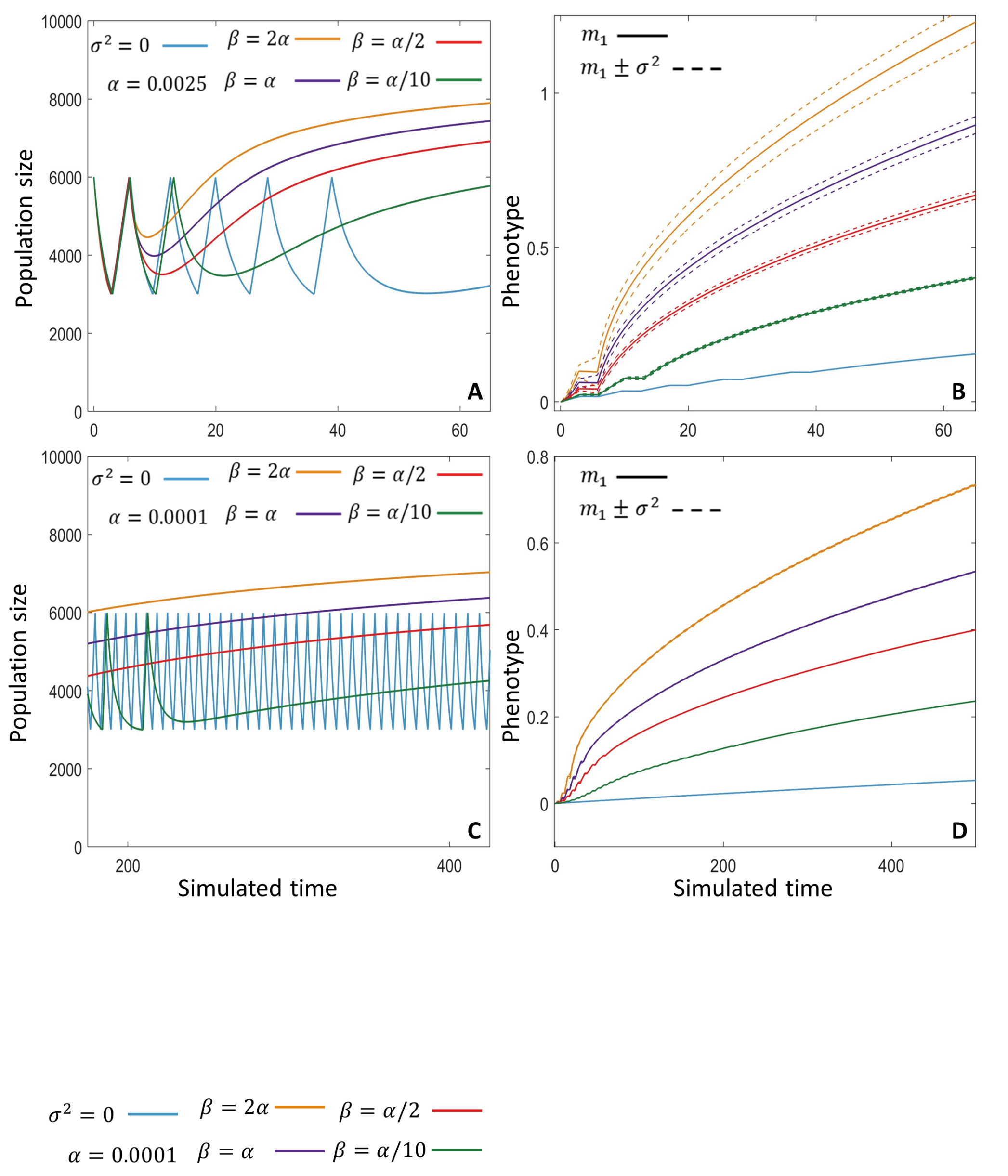
Figure 1: A comparison between the adaptive dynamics model including and excluding population heterogeneity during simulated adaptive therapy as implemented by Pressley et al., [66]. Panel A shows the simulated tumour dynamics, $P(t)$, for Eq. (26) in blue, denoted by $\sigma^{2}=0$. The remaining curves in panel A represent the population dynamics obtained by including population heterogeneity as in Eq. (29) for four distinct diffusion rates $\beta$. Panel B shows the corresponding predicted mean phenotype, $m_{1}(t)$. In all cases, the mean phenotype is plotted in a solid line, while the variance is shown in dashed lines for the four simulations that include population heterogeneity. Panel C shows a long-term simulation of adaptive therapy for $\alpha=0.0001$. For clarity, we only show $t\in(175,425)$ in panel C; the tumours with the 3 largest diffusion coefficients, $\beta$, have already developed resistance. The complete phenotypic dynamics for this long-term simulation are shown in panel D. Other than the given value of $\alpha,$ all simulations used the parameter values given in Pressley et al., [66].

In panel A of Fig 1, we note that population heterogeneity, even for small diffusion rates $\beta$, drives the development of resistance and tumour progression faster than in the model without population heterogeneity. Furthermore, the mean phenotype, $m_{1}$, is larger in the simulations including population heterogeneity, obtained from Eq. (29), than in those for the model of Pressley et al., [66], obtained from Eq. (26), at any given time. This highlights that population diversity may accelerate the development of treatment resistance as has been observed in many experimental [10, 60, 9, 76, 57, 33] and theoretical studies [3, 2, 6, 55, 83, 50, 89, 49, 19, 79, 44, 53, 41, 62]. To test the role of population heterogeneity in treatment outcome, we performed a longer-term simulations with $\alpha=0.0001$, as illustrated in panels C and D of Fig 1. In all cases that account for population heterogeneity, Eq. (29) predicts the evolution of resistance and failure of adaptive therapy. Conversely, the model neglecting phenotypic diversity instead predicts long-term control of tumour growth.

5 Discussion

Mathematical models have become increasingly important in our understanding of the mechanisms driving cancer evolutionary dynamics and the role of intratumour phenotypic heterogeneity. Phenotype-structured PDE models describe the temporal dynamics of both the tumour size and phenotypic composition. In the context of adaptive dynamics in continuously structured phenotypic space, these PDE models carry a distinct advantage in that individual model terms are directly biologically interpretable.

Benefits of reducing a phenotype-structured PDE to a system of ODEs.

While phenotype-structured PDE models are well-poised to interpret biological data, they carry, by their very nature, challenges that do not apply to the ODE models that are routine in the interpretation of data. For example, for a mathematical model to be parameterised it must be identifiable [8, 67, 17]. Outside of recent work [13, 11, 78], most computational tools for parameter identifiability analysis are developed for ODE models [8, 67]. Therefore, assessing parameter identifiability in PDE models often requires an ODE surrogate such as an equivalent or approximate system of moment equations [14]. Parameter identifiability is particularly pertinent in the case of phenotype-structured PDE models, as determining the phenotypic distribution of a tumour sample is experimentally demanding [12, 65]. Furthermore, numerical methods for phenotype-structured PDEs are not widely implemented in existing scientific software [68, 16]. Consequently, fitting these PDE models to experimental data often requires the development of problem specific software. The resulting numerical methods are typically more computationally expensive than for ODE models, with an increase in cost that becomes prohibitive as the dimensionality of the problem increases. Therefore, the ability to reduce a phenotype-structured PDE to a system of ODEs while maintaining the ability to characterise the tumour composition allows for significant computational efficiency.

Summary and novelty of our model-reduction procedure.

Accordingly, we proposed a generalised method to reduce a phenotype-structured PDE model of cancer adaptive dynamics to a system of ODEs for the moments of the phenotypic distribution, up to an arbitrary number of moments. This reduction allows modellers to use existing technical tools for ODE models while maintaining the biological relevance and the interpretability of the phenotype-structured PDE. The model-reduction procedure we propose relies on the use of the moment generating function of the phenotypic distribution, a Taylor series expansion of the phenotypic drift and proliferation rate functions, and truncation closure. Our work extends the analysis of Almeida et al., [2] and Chisholm et al., 2016b [27], to a more biologically relevant phenotypic domain and a model without any a priori assumptions on the shape of the distribution or the dependency of the phenotypic drift and proliferation rate on the phenotypic trait. Our work also extends the analysis of Dieckmann and Law, [35] that ties a stochastic model of mutation-selection dynamics to the adaptive dynamics models in Section 4.2.

Strengths and limitations.

Our model reduction procedure is independent of both the shape of the phenotypic distribution and the functional form of the terms that characterise adaptation. This generality and flexibility lends our analysis suitable for adaptation in a wide range of contexts, both within mathematical oncology and more broadly. We expect many of the advantages conferred by the reduced model to become even more pertinent in high-dimensional phenotypic spaces, particularly in the context of mechanistic interpretation of correspondingly high-dimensional multi-omics data. The necessity to impose a system closure yields an approximation of the underlying dynamics. However, we highlight that the presented approach can be applied up to an arbitrary order. The question of how many moments a problem necessitates, the closure to apply, or the effect of closure on parameter identifiability, remains open even in fields where moment closures have a long history [75, 51, 38, 69, 14, 87]. We expect unimodal phenotypic distributions to be well characterised by lower-order moments and our truncation closure. For high-dimensional problems, the question of closure type and order is likely determined by computational cost. Ultimately, we provide a general and flexible framework for describing adaptation in a continuously-distributed phenotypic space whilst retaining the computational and analytical advantages of ODE-based approaches.

Consequences and perspectives in cancer adaptive therapy.

Our work relaxes the assumptions of near-linear growth rates or vanishing variance underlying the canonical equation of adaptive dynamics [35] by explicitly linking the higher-order moments of the population distribution in phenotypic space with the resulting impacts on population growth and adaptation. To illustrate the possible effects of including population heterogeneity, we considered the model of adaptive dynamics in response to adaptive therapy by Pressley et al., [66]. We show that the inclusion of population heterogeneity can lead to treatment failure, under the same representative model parameters used in [66], whereas the opposite outcome was observed by the authors. While this result is unsurprising [10], it illustrates how phenotypic instability, manifested as population phenotypic heterogeneity, can drive tumour evolution [1, 43].

In this context, our work is directly relevant to recent multi-omics-level experiments characterising cellular phenotypes. However, these high dimensional data sets are challenging to interpret and thus numerous dimensionality reduction methods have been proposed [63, 15]. Amongst these are phenotype classification methods that summarise these data sets with a selected number of moments [86, 80]. As such, moment-based descriptions are increasingly considered to describe phenotypic states and our modelling therefore offers a direct link with these emerging clinically relevant data sets. For example, bulk and single-cell sequencing has identified continuous phenotypic adaptation in response to treatments in patient-derived xenografts carrying the BRAFV600E mutation [90]. Consequently, the framework derived in this work could facilitate both the development of mathematical models and the calibration of these models by multi-omics data to understand how phenotypic heterogeneity drives the evolution of treatment resistance to targeted therapies.

Code availability

The Matlab code underlying the simulations in Section 4.2 is available at https://github.com/ttcassid//Phenotype$\_$Continuous$\_$Adaptation

References

- Aguadé-Gorgorió and Solé, [2018] Aguadé-Gorgorió, G. and Solé, R. (2018). Adaptive dynamics of unstable cancer populations: The canonical equation. Evol. Appl., 11(8):1283–1292.
- Almeida et al., [2019] Almeida, L., Bagnerini, P., Fabrini, G., Hughes, B. D., and Lorenzi, T. (2019). Evolution of cancer cell populations under cytotoxic therapy and treatment optimisation: insight from a phenotype-structured model. ESAIM: Math. Model Num., 53(4):1157–1190.
- Almeida et al., [2024] Almeida, L., Denis, J. A., Ferrand, N., Lorenzi, T., Prunet, A., Sabbah, M., and Villa, C. (2024). Evolutionary dynamics of glucose-deprived cancer cells: insights from experimentally informed mathematical modelling. J. R. Soc. Interface, 21(210):20230587.
- Altrock et al., [2015] Altrock, P. M., Liu, L. L., and Michor, F. (2015). The mathematics of cancer: integrating quantitative models. Nat. Rev. Cancer, 15(12):730–745.
- Anderson et al., [2006] Anderson, A. R., Weaver, A. M., Cummings, P. T., and Quaranta, V. (2006). Tumor Morphology and Phenotypic Evolution Driven by Selective Pressure from the Microenvironment. Cell, 127(5):905–915.
- Ardaševa et al., [2020] Ardaševa, A., Gatenby, R. A., Anderson, A. R., Byrne, H. M., Maini, P. K., and Lorenzi, T. (2020). Evolutionary dynamics of competing phenotype-structured populations in periodically fluctuating environments. J. Math. Biol., 80:775–807.
- Bell and Gilan, [2020] Bell, C. C. and Gilan, O. (2020). Principles and mechanisms of non-genetic resistance in cancer. Br. J. Cancer, 122(4):465–472.
- Bellman and Åström, [1970] Bellman, R. and Åström, K. (1970). On structural identifiability. Math. Biosci., 7(3-4):329–339.
- Biswas et al., [2023] Biswas, A., Sahoo, S., Riedlinger, G. M., Ghodoussipour, S., Jolly, M. K., and De, S. (2023). Transcriptional state dynamics lead to heterogeneity and adaptive tumor evolution in urothelial bladder carcinoma. Commun. Biol., 6(1):1292.
- Bódi et al., [2017] Bódi, Z., Farkas, Z., Nevozhay, D., Kalapis, D., Lázár, V., Csörgö, B., Nyerges, Á., Szamecz, B., Fekete, G., Papp, B., Araújo, H., Oliveira, J. L., Moura, G., Santos, M. A. S., Székely Jr, T., Balázsi, G., and Pál, C. (2017). Phenotypic heterogeneity promotes adaptive evolution. PLOS Biol., 15(5):e2000644.
- Boiger et al., [2016] Boiger, R., Hasenauer, J., Hroß, S., and Kaltenbacher, B. (2016). Integration based profile likelihood calculation for PDE constrained parameter estimation problems. Inverse Probl., 32(12):125009.
- Brestoff and Frater, [2022] Brestoff, J. R. and Frater, J. L. (2022). Contemporary challenges in clinical flow cytometry: small samples, big data, little time. JALM, 7(4):931–944.
- Browning et al., [2024] Browning, A. P., Taşcă, M., Falcó, C., and Baker, R. E. (2024). Structural identifiability analysis of linear reaction–advection–diffusion processes in mathematical biology. P. R. Soc. A, 480(2286):20230911.
- Browning et al., [2020] Browning, A. P., Warne, D. J., Burrage, K., Baker, R. E., and Simpson, M. J. (2020). Identifiability analysis for stochastic differential equation models in systems biology. J. R. Soc. Interface, 17:20200652.
- Burkhardt et al., [2022] Burkhardt, D. B., San Juan, B. P., Lock, J. G., Krishnaswamy, S., and Chaffer, C. L. (2022). Mapping phenotypic plasticity upon the cancer cell state landscape using manifold learning. Cancer Discov., 12(8):1847–1859.
- Carpenter et al., [2017] Carpenter, B., Gelman, A., Hoffman, M. D., Lee, D., Goodrich, B., Betancourt, M., Brubaker, M., Guo, J., Li, P., and Riddell, A. (2017). Stan: a probabilistic programming language. J. Stat. Softw., 76(1).
- Cassidy, [2023] Cassidy, T. (2023). A continuation technique for maximum likelihood estimators in biological models. Bull. Math. Biol., 85(10):90.
- Cassidy and Craig, [2019] Cassidy, T. and Craig, M. (2019). Determinants of combination GM-CSF immunotherapy and oncolytic virotherapy success identified through in silico treatment personalization. PLOS Comput. Biol., 15(11):e1007495.
- Cassidy and Humphries, [2019] Cassidy, T. and Humphries, A. R. (2019). A mathematical model of viral oncology as an immuno-oncology instigator. Math. Med. Biol. A J. IMA, 37(1):117–151.
- Cassidy et al., [2021] Cassidy, T., Nichol, D., Robertson-Tessi, M., Craig, M., and Anderson, A. R. A. (2021). The role of memory in non-genetic inheritance and its impact on cancer treatment resistance. PLOS Comput. Biol., 17(8):e1009348.
- Celora et al., [2022] Celora, G. L., Bader, S. B., Hammond, E. M., Maini, P. K., Pitt-Francis, J. M., and Byrne, H. M. (2022). A dna-structured mathematical model of cell-cycle progression in cyclic hypoxia. J. Theor. Biol., 545:111104.
- Celora et al., [2021] Celora, G. L., Byrne, H. M., Zois, C. E., and Kevrekidis, P. G. (2021). Phenotypic variation modulates the growth dynamics and response to radiotherapy of solid tumours under normoxia and hypoxia. J. Theor. Biol., 527:110792.
- Champagnat et al., [2002] Champagnat, N., Ferričre, R., and Ben Arous4, G. (2002). The canonical equation of adaptive dynamics: a mathematical view. Selection, 2(1-2):73–83.
- Champagnat et al., [2006] Champagnat, N., Ferrière, R., and Méléard, S. (2006). Unifying evolutionary dynamics: from individual stochastic processes to macroscopic models. Theor. Popul. Biol., 69(3):297–321.
- Chen et al., [2023] Chen, J.-Y., Hug, C., Reyes, J., Tian, C., Gerosa, L., Fröhlich, F., Ponsioen, B., Snippert, H. J., Spencer, S. L., Jambhekar, A., Sorger, P. K., and Lahav, G. (2023). Multi-range ERK responses shape the proliferative trajectory of single cells following oncogene induction. Cell Rep., 42(3):112252.
- [26] Chisholm, R. H., Lorenzi, T., and Clairambault, J. (2016a). Cell population heterogeneity and evolution towards drug resistance in cancer: biological and mathematical assessment, theoretical treatment optimisation. Biochim. Biophys. Acta, 1860(11):2627–2645.
- [27] Chisholm, R. H., Lorenzi, T., Desvillettes, L., and Hughes, B. D. (2016b). Evolutionary dynamics of phenotype-structured populations: from individual-level mechanisms to population-level consequences. Z Angew. Math. Me., 67:1–34.
- Chisholm et al., [2015] Chisholm, R. H., Lorenzi, T., Lorz, A., Larsen, A. K., De Almeida, L. N., Escargueil, A., and Clairambault, J. (2015). Emergence of Drug Tolerance in Cancer Cell Populations: An Evolutionary Outcome of Selection, Nongenetic Instability, and Stress-Induced Adaptation. Cancer Res., 75(6):930–939.
- [29] Cho, H. and Levy, D. (2018a). Modeling continuous levels of resistance to multidrug therapy in cancer. Appl. Math. Model., 64:733–751.
- [30] Cho, H. and Levy, D. (2018b). Modeling the chemotherapy-induced selection of drug-resistant traits during tumor growth. J. Theor. Biol., 436:120–134.
- Clairambault and Pouchol, [2019] Clairambault, J. and Pouchol, C. (2019). A survey of adaptive cell population dynamics models of emergence of drug resistance in cancer, and open questions about evolution and cancer. Biomath,, 8(1):23.
- Coggan and Page, [2022] Coggan, H. and Page, K. M. (2022). The role of evolutionary game theory in spatial and non-spatial models of the survival of cooperation in cancer: a review. J. R. Soc. Interface, 19(193).
- Craig et al., [2019] Craig, M., Kaveh, K., Woosley, A., Brown, A. S., Goldman, D., Eton, E., Mehta, R. M., Dhawan, A., Arai, K., Rahman, M. M., Chen, S., Nowak, M. A., and Goldman, A. (2019). Cooperative adaptation to therapy (CAT) confers resistance in heterogeneous non-small cell lung cancer. PLOS Comput. Biol., 15(8):e1007278.
- Curto and di Dio, [2023] Curto, R. E. and di Dio, P. J. (2023). Time-dependent moments from the heat equation and a transport equation. Int. Math. Res. Not., 2023(17):14955–14990.
- Dieckmann and Law, [1996] Dieckmann, U. and Law, R. (1996). The dynamical theory of coevolution: a derivation from stochastic ecological processes. J. Math. Biol., 34(5-6):579–612.
- Engblom, [2006] Engblom, S. (2006). Computing the moments of high dimensional solutions of the master equation. Appl. Math. Comput., 180(2):498–515.
- Fan et al., [2016] Fan, S., Geissmann, Q., Lakatos, E., Lukauskas, S., Ale, A., Babtie, A. C., Kirk, P. D. W., and Stumpf, M. P. H. (2016). MEANS: python package for Moment Expansion Approximation, iNference and Simulation. Bioinformatics, 32(18):2863–2865.
- Ghusinga et al., [2017] Ghusinga, K. R., Soltani, M., Lamperski, A., Dhople, S. V., and Singh, A. (2017). Approximate moment dynamics for polynomial and trigonometric stochastic systems. In 2017 IEEE 56th Annual Conference on Decision and Control (CDC), pages 1864–1869. IEEE.
- Gillespie, [2009] Gillespie, C. S. (2009). Moment-closure approximations for mass-action models. IET Syst. Biol., 3(1):52–58.
- Goldman et al., [2015] Goldman, A., Majumder, B., Dhawan, A., Ravi, S., Goldman, D., Kohandel, M., Majumder, P. K., and Sengupta, S. (2015). Temporally sequenced anticancer drugs overcome adaptive resistance by targeting a vulnerable chemotherapy-induced phenotypic transition. Nat. Commun., 6(1):6139.
- Greene et al., [2014] Greene, J., Lavi, O., Gottesman, M. M., and Levy, D. (2014). The impact of cell density and mutations in a model of multidrug resistance in solid tumors. Bull. Math. Biol., 76(3):627–653.
- Gunnarsson et al., [2020] Gunnarsson, E. B., De, S., Leder, K., and Foo, J. (2020). Understanding the role of phenotypic switching in cancer drug resistance. J. Theor. Biol., 490:110162.
- Hanahan, [2022] Hanahan, D. (2022). Hallmarks of cancer: new dimensions. Cancer Discov., 12(1):31–46.
- Iwasa et al., [2006] Iwasa, Y., Nowak, M. A., and Michor, F. (2006). Evolution of resistance during clonal expansion. Genetics, 172(4):2557–2566.
- Kadanoff, [2000] Kadanoff, L. P. (2000). Statistical Physics: Statics, Dynamics And Renormalization. World Scientific, Singapore. Includes bibliographical references and index.
- Kareva, [2022] Kareva, I. (2022). Different costs of therapeutic resistance in cancer: Short- and long-term impact of population heterogeneity. Math. Biosci., 352(June):108891.
- Kavran et al., [2022] Kavran, A. J., Stuart, S. A., Hayashi, K. R., Basken, J. M., Brandhuber, B. J., and Ahn, N. G. (2022). Intermittent treatment of BRAFV600E melanoma cells delays resistance by adaptive resensitization to drug rechallenge. Proc. Natl. Acad. Sci. U. S. A., 119(12).
- Kaznatcheev et al., [2019] Kaznatcheev, A., Peacock, J., Basanta, D., Marusyk, A., and Scott, J. G. (2019). Fibroblasts and alectinib switch the evolutionary games played by non-small cell lung cancer. Nat. Ecol. Evol., 3(3):450–456.
- Köhn-Luque et al., [2023] Köhn-Luque, A., Myklebust, E. M., Tadele, D. S., Giliberto, M., Schmiester, L., Noory, J., Harivel, E., Arsenteva, P., Mumenthaler, S. M., Schjesvold, F., Taskén, K., Enserink, J. M., Leder, K., Frigessi, A., and Foo, J. (2023). Phenotypic deconvolution in heterogeneous cancer cell populations using drug-screening data. Cell Rep. Methods, page 100417.
- Kucharavy et al., [2018] Kucharavy, A., Rubinstein, B., Zhu, J., and Li, R. (2018). Robustness and evolvability of heterogeneous cell populations. Mol. Biol. Cell, 29(11):1400–1409.
- Kuehn, [2016] Kuehn, C. (2016). Moment Closure—A Brief Review. In Control of Self-Organizing Nonlinear Systems, pages 253–271. Springer.
- Labrie et al., [2022] Labrie, M., Brugge, J. S., Mills, G. B., and Zervantonakis, I. K. (2022). Therapy resistance: opportunities created by adaptive responses to targeted therapies in cancer. Nat. Rev. Cancer, 22(6):323–339.
- Lavi et al., [2013] Lavi, O., Greene, J. M., Levy, D., and Gottesman, M. M. (2013). The role of cell density and intratumoral heterogeneity in multidrug resistance. Cancer Res., 73(24):7168–7175.
- Lee et al., [2009] Lee, C. H., Kim, K.-H., and Kim, P. (2009). A moment closure method for stochastic reaction networks. J. Chem. Phys., 130(13).
- Lorenzi et al., [2015] Lorenzi, T., Chisholm, R. H., Desvillettes, L., and Hughes, B. D. (2015). Dissecting the dynamics of epigenetic changes in phenotype-structured populations exposed to fluctuating environments. J. Theor. Biol., 386:166–176.
- Lorenzi et al., [2020] Lorenzi, T., Macfarlane, F. R., and Villa, C. (2020). Discrete and continuum models for the evolutionary and spatial dynamics of cancer: a very short introduction through two case studies. In Trends in Biomathematics: Modeling Cells, Flows, Epidemics, and the Environment, pages 359–380. Springer.
- Marine et al., [2020] Marine, J.-C., Dawson, S.-J., and Dawson, M. A. (2020). Non-genetic mechanisms of therapeutic resistance in cancer. Nat. Rev. Cancer.
- Martinez et al., [2021] Martinez, V. A., Laleh, N. G., Salvioli, M., Thuijsman, F., Brown, J. S., Cavill, R., Kather, J. N., and Staňková, K. (2021). Improving mathematical models of cancer by including resistance to therapy: a study in non-small cell lung cancer. bioRxiv, pages 1–27.
- Marusyk et al., [2020] Marusyk, A., Janiszewska, M., and Polyak, K. (2020). Intratumor heterogeneity: the rosetta stone of therapy resistance. Cancer cell, 37(4):471–484.
- McGranahan and Swanton, [2017] McGranahan, N. and Swanton, C. (2017). Clonal heterogeneity and tumor evolution: past, present, and the future. Cell, 168(4):613–628.
- Mosier et al., [2021] Mosier, J. A., Schwager, S. C., Boyajian, D. A., and Reinhart-King, C. A. (2021). Cancer cell metabolic plasticity in migration and metastasis. Clin. Exp. Metastasis, 38(4):343–359.
- Nichol et al., [2016] Nichol, D., Robertson-Tessi, M., Jeavons, P., and Anderson, A. R. (2016). Stochasticity in the genotype-phenotype map: implications for the robustness and persistence of bet-hedging. Genetics, 204(4):1523–1539.
- Oshternian et al., [2024] Oshternian, S. R., Loipfinger, S., Bhattacharya, A., and Fehrmann, R. S. N. (2024). Exploring combinations of dimensionality reduction, transfer learning, and regularization methods for predicting binary phenotypes with transcriptomic data. BMC Bioinformatics, 25(1):167.
- Perthame and Barles, [2008] Perthame, B. and Barles, G. (2008). Dirac concentrations in Lotka-Volterra parabolic PDEs. Indiana U. Math. J., pages 3275–3301.
- Pigliucci, [2010] Pigliucci, M. (2010). Genotype-phenotype mapping and the end of the ‘genes as blueprint’ metaphor. Philos. Trans. R. Soc. B, 365(1540):557–566.
- Pressley et al., [2021] Pressley, M., Salvioli, M., Lewis, D. B., Richards, C. L., Brown, J. S., and Staňková, K. (2021). Evolutionary dynamics of treatment-induced resistance in cancer informs understanding of rapid evolution in natural systems. Front. Ecol. Evol., 9(August):1–22.
- Raue et al., [2009] Raue, A., Kreutz, C., Maiwald, T., Bachmann, J., Schilling, M., Klingmüller, U., and Timmer, J. (2009). Structural and practical identifiability analysis of partially observed dynamical models by exploiting the profile likelihood. Bioinformatics, 25(15):1923–1929.
- Sas, [2020] Sas, L. (2020). Monolix.
- Schnoerr et al., [2017] Schnoerr, D., Sanguinetti, G., and Grima, R. (2017). Approximation and inference methods for stochastic biochemical kinetics—a tutorial review. J. Phys. A, 50(9):093001.
- Shaffer et al., [2017] Shaffer, S. M., Dunagin, M. C., Torborg, S. R., Torre, E. A., Emert, B., Krepler, C., Beqiri, M., Sproesser, K., Brafford, P. A., Xiao, M., Eggan, E., Anastopoulos, I. N., Vargas-Garcia, C. A., Singh, A., Nathanson, K. L., Herlyn, M., and Raj, A. (2017). Rare cell variability and drug-induced reprogramming as a mode of cancer drug resistance. Nature, 546(7658):431–435.
- Sharma et al., [2010] Sharma, S. V., Lee, D. Y., Li, B., Quinlan, M. P., Takahashi, F., Maheswaran, S., McDermott, U., Azizian, N., Zou, L., Fischbach, M. A., Wong, K. K., Brandstetter, K., Wittner, B., Ramaswamy, S., Classon, M., and Settleman, J. (2010). A chromatin-mediated reversible drug-tolerant state in cancer cell subpopulations. Cell, 141(1):69–80.
- Shen and Clairambault, [2020] Shen, S. and Clairambault, J. (2020). Cell plasticity in cancer cell populations. F1000Research, 9.
- Shi et al., [2023] Shi, Z.-D., Pang, K., Wu, Z.-X., Dong, Y., Hao, L., Qin, J.-X., Wang, W., Chen, Z.-S., and Han, C.-H. (2023). Tumor cell plasticity in targeted therapy-induced resistance: mechanisms and new strategies. Signal Transduct. Target. Ther., 8(1):113.
- Smalley et al., [2019] Smalley, I., Kim, E., Li, J., Spence, P., Wyatt, C. J., Eroglu, Z., Sondak, V. K., Messina, J. L., Babacan, N. A., Maria-Engler, S. S., et al. (2019). Leveraging transcriptional dynamics to improve braf inhibitor responses in melanoma. EBioMedicine, 48:178–190.
- Smith et al., [2007] Smith, S., Fox, R., and Raman, V. (2007). A quadrature closure for the reaction-source term in conditional-moment closure. Proc. Combust. Inst., 31(1):1675–1682.
- Sottoriva et al., [2013] Sottoriva, A., Spiteri, I., Piccirillo, S. G. M., Touloumis, A., Collins, V. P., Marioni, J. C., Curtis, C., Watts, C., and Tavaré, S. (2013). Intratumor heterogeneity in human glioblastoma reflects cancer evolutionary dynamics. Proc. Natl. Acad. Sci. U. S. A., 110(10):4009–4014.
- Stace et al., [2020] Stace, R. E., Stiehl, T., Chaplain, M. A., Marciniak-Czochra, A., and Lorenzi, T. (2020). Discrete and continuum phenotype-structured models for the evolution of cancer cell populations under chemotherapy. Math. Model. Nat. Phenom., 15:14.
- Stapor et al., [2018] Stapor, P., Weindl, D., Ballnus, B., Hug, S., Loos, C., Fiedler, A., Krause, S., Hroß, S., Fröhlich, F., and Hasenauer, J. (2018). PESTO: Parameter EStimation TOolbox. Bioinformatics, 34(4):705–707.
- Sun et al., [2016] Sun, X., Bao, J., and Shao, Y. (2016). Mathematical modeling of therapy-induced cancer drug resistance: connecting cancer mechanisms to population survival rates. Sci. Rep., 6(1):22498.
- Tang et al., [2010] Tang, K. L., Li, T. H., Xiong, W. W., and Chen, K. (2010). Ovarian cancer classification based on dimensionality reduction for SELDI-TOF data. BMC Bioinformatics, 11:109.
- Tasdogan et al., [2020] Tasdogan, A., Faubert, B., Ramesh, V., Ubellacker, J. M., Shen, B., Solmonson, A., Murphy, M. M., Gu, Z., Gu, W., Martin, M., et al. (2020). Metabolic heterogeneity confers differences in melanoma metastatic potential. Nature, 577(7788):115–120.
- Tirosh et al., [2016] Tirosh, I., Izar, B., Prakadan, S. M., Wadsworth, M. H., Treacy, D., Trombetta, J. J., Rotem, A., Rodman, C., Lian, C., Murphy, G., Fallahi-Sichani, M., Dutton-Regester, K., Lin, J.-R., Cohen, O., Shah, P., Lu, D., Genshaft, A. S., Hughes, T. K., Ziegler, C. G. K., Kazer, S. W., Gaillard, A., Kolb, K. E., Villani, A.-C., Johannessen, C. M., Andreev, A. Y., Van Allen, E. M., Bertagnolli, M., Sorger, P. K., Sullivan, R. J., Flaherty, K. T., Frederick, D. T., Jané-Valbuena, J., Yoon, C. H., Rozenblatt-Rosen, O., Shalek, A. K., Regev, A., and Garraway, L. A. (2016). Dissecting the multicellular ecosystem of metastatic melanoma by single-cell RNA-seq. Science, 352(6282):189–196.
- Villa et al., [2021] Villa, C., Chaplain, M. A., and Lorenzi, T. (2021). Evolutionary dynamics in vascularised tumours under chemotherapy: Mathematical modelling, asymptotic analysis and numerical simulations. Vietnam J. Math., 49:143–167.
- Vincent and Brown, [2005] Vincent, T. L. and Brown, J. S. (2005). Evolutionary Game Theory, Natural Selection, and Darwinian Dynamics. Cambridge University Press.
- Vincent and Gatenby, [2008] Vincent, T. L. and Gatenby, R. A. (2008). An evolutionary model for initiation, promotion, and progression in carcinogenesis. Int. J. Oncol., 32(4):729–37.
- Vogelstein et al., [2021] Vogelstein, J. T., Bridgeford, E. W., Tang, M., Zheng, D., Douville, C., Burns, R., and Maggioni, M. (2021). Supervised dimensionality reduction for big data. Nat. Commun., 12(1):2872.
- Wagner et al., [2022] Wagner, V., Castellaz, B., Oesting, M., and Radde, N. (2022). Quasi-entropy closure: a fast and reliable approach to close the moment equations of the chemical master equation. Bioinformatics, 38(18):4352–4359.
- West et al., [2018] West, J., Ma, Y., and Newton, P. K. (2018). Capitalizing on competition: An evolutionary model of competitive release in metastatic castration resistant prostate cancer treatment. J. Theor. Biol., 455:249–260.
- Wooten and Quaranta, [2017] Wooten, D. J. and Quaranta, V. (2017). Mathematical models of cell phenotype regulation and reprogramming: Make cancer cells sensitive again! Biochim. Biophys. Acta, 1867(2):167–175.
- Xue et al., [2017] Xue, Y., Martelotto, L., Baslan, T., Vides, A., Solomon, M., Mai, T. T., Chaudhary, N., Riely, G. J., Li, B. T., Scott, K., Cechhi, F., Stierner, U., Chadalavada, K., de Stanchina, E., Schwartz, S., Hembrough, T., Nanjangud, G., Berger, M. F., Nilsson, J., Lowe, S. W., Reis-Filho, J. S., Rosen, N., and Lito, P. (2017). An approach to suppress the evolution of resistance in BRAFV600E-mutant cancer. Nat. Med., 23(8):929–937.