A modified dyon solution in a non-Abelian gauge model

Abstract

A modified $SU(2)$ Georgi-Glashow model is considered here, and it is shown that besides the well-known Julia-Zee dyon solution, the model can also have a modified dyon solution. The properties of the modified dyon solution are studied using analytical and numerical methods. A comparative analysis of the modified dyon and the Julia-Zee dyon shows that their properties are significantly different. In particular, except for the BPS case, the energy and electric charge of the modified dyons exceed considerably those of the Julia-Zee dyons. At the same time, the energy and electric charge of the modified dyon are bounded for all admissible parameter values, whereas those of the Julia-Zee dyon can be arbitrarily large in the BPS case.

1 Introduction

Among the various soliton solutions of field theory, there are those that have an electric charge. These soliton solutions can exist in both $(2+1)$-dimensional [1, 2, 3, 4, 5, 6, 7, 8, 9, 10, 11, 12] and $(3+1)$-dimensional [13, 14, 15, 16, 17, 18, 19, 20, 21, 22, 23, 24, 25, 26] gauge models. To ensure the finiteness of the energy of two-dimensional electrically charged solitons, $(2+1)$-dimensional gauge models must include the Chern-Simons term [27, 28, 29], whereas the Maxwell term may be missing. Due to the Chern-Simons term, the gauge field in these models is topologically massive, and therefore the electric field of the solitons is short-range. In contrast, the electric field of three-dimensional solitons is long-range, since there is no Chern-Simons term in $(3+1)$ dimensions and the gauge field models include only the Maxwell term.

The electrically charged solitons can be divided into two classes: topological solitons [13, 14, 15, 16, 17] and nontopological solitons [18, 19, 20, 21, 22, 23, 24, 25, 26]. The properties of the topological and nontopological solitons are considerably different. Because of topological triviality, the existence of nontopological solitons is entirely due to dynamical factors. In particular, a conserved Noether charge must exist in the corresponding field model, and the self-interaction potential of the scalar fields has to be of a special form [30, 31]. For a fixed value of the Noether charge, the field configuration of a nontopological soliton is a stationary point of the energy functional [32, 33, 34]. As a consequence, the energy and the Noether charge of the nontopological soliton are related by a differential relation, which determines a number of the soliton’s properties.

In contrast, topological solitons have topologically nontrivial field configurations, which prevents them from transitioning into lower energy states [35]. Hence, the presence of a potential term and Noether charge is not a necessary condition for the existence of three-dimensional topological solitons, as can be seen in the example of the BPS monopole [14]. The best known example of an electrically charged three-dimensional topological soliton is the dyon solution [13] in the $SU(2)$ Georgi-Glashow model [36]. Similar to nontopological solitons, a dyon solution is a stationary point (minimum) of the energy functional for a fixed value of the Noether (electric) charge. It follows that the the energy and the electric charge of the dyon are also related by a differential relation [37], as is the case for the nontopological solitons. As a result, except for the BPS case, the energy and electric charge of the dyon cannot be arbitrarily large [16].

In [38, 39], a soliton system consisting of vortex and Q-ball components interacting via an electric field is described. Being a source of an electric field, a dyon can also interact with another charged field, as a result of which a new soliton system can arise. In this paper, we consider a soliton system (modified dyon) arising from the interaction of the Julia-Zee dyon [13] and an isospinor self-interacting scalar field. The modified dyon consists of a core (deformed Julia-Zee dyon) surrounded by a cloud of a charged scalar field, and its properties differ significantly from those of the Julia-Zee dyon.

Throughout this paper, we use the natural units $c=1$, $\hbar=1$.

2 Lagrangian and field equations of the model

We consider a modified Georgi-Glashow model with a non-Abelian gauge group $SU(2)$. The model contains two types of self-interacting scalar fields, one of which is transformed according to the adjoint representation of the gauge group $SU(2)$, and the other according to the fundamental representation. The Lagrangian of the model takes the form

$$\mathcal{L} =-\frac{1}{4}F_{\mu\nu}^{a}F^{a\,\mu\nu}+\frac{1}{2}\left(D_{\mu}\phi^{a}\right)\left(D^{\mu}\phi^{a}\right)$$

$$+\left(D_{\mu}\Phi\right)^{{\dagger}}\left(D^{\mu}\Phi\right)-V\left(\phi^{a}\phi^{a}\right)-U\left(\Phi^{{\dagger}}\Phi\right),$$ (1)

where

$$F_{\mu\nu}^{a}=\partial_{\mu}A_{\nu}^{a}-\partial_{\nu}A_{\mu}^{a}-g\epsilon^{abc}A_{\mu}^{b}A_{\nu}^{c}$$ (2)

is the non-Abelian field strength,

$$D_{\mu}\phi^{a}=\partial_{\mu}\phi^{a}-g\epsilon^{abc}A_{\mu}^{b}\phi^{c}$$ (3)

is the covariant derivative of the isovector scalar field $\boldsymbol{\phi}$, and

$$D_{\mu}\Phi=\partial_{\mu}\Phi+igA_{\mu}^{a}\frac{\tau_{a}}{2}\Phi$$ (4)

is the covariant derivative of the isospinor scalar field $\Phi$. The self-interaction potentials of the isovector and isospinor scalar fields are

$$V\left(\phi^{a}\phi^{a}\right)=\frac{\lambda}{4}\left(\phi^{a}\phi^{a}-v^{2}\right)^{2}$$ (5)

and

$$U\left(\Phi^{{\dagger}}\Phi\right)=M^{2}\Phi^{{\dagger}}\Phi-\frac{G}{2}\left(\Phi^{{\dagger}}\Phi\right)^{2}+\frac{H}{3}\left(\Phi^{{\dagger}}\Phi\right)^{3},$$ (6)

respectively, where $M$ is a mass parameter, and $\lambda$, $G$, and $H$ are coupling constants. Note that the six-order potential in Eq. (6) is of the form widely used in models having Q-ball solutions.

Eq. (5) tells us that the potential $V$ reaches a zero minimum value at non-zero $\left|\boldsymbol{\phi}\right|=v$. At the same time, we assume that the potential $U$ has a global minimum at $\Phi=0$. For this to hold, the parameters of the potential $U$ in Eq. (6) must satisfy the inequality $3G^{2}<16HM^{2}$. The nonzero vacuum value of the isovector scalar field $\boldsymbol{\phi}$ leads to a spontaneous violation of the gauge group $SU(2)$ to an Abelian (electromagnetic) subgroup $U(1)$. As a result of the Higgs mechanism, the spectrum of small fluctuations of fields relative to the vacuum contains one neutral massless vector field, two charged massive vector fields with mass $m_{V}=gv$, one neutral massive Higgs field with mass $m_{H}=\sqrt{2\lambda}v$, and two charged massive scalar fields with mass $m_{\Phi}=M$.

Using standard methods of field theory, we find the field equations of model: (1)

$$D_{\mu}F^{a\,\mu\nu}=J^{a\,\nu},$$ (7)

$$D_{\mu}D^{\mu}\phi^{a}=-\lambda\left(\phi^{b}\phi^{b}-v^{2}\right)\phi^{a},$$ (8)

$$D_{\mu}D^{\mu}\Phi=-\left[M^{2}-G\left(\Phi^{{\dagger}}\Phi\right)+H\left(\Phi^{{\dagger}}\Phi\right)^{2}\right]\Phi,$$ (9)

where the covariantly conserved current

$$J^{a\,\nu} =g\epsilon_{abc}\phi_{b}D^{\nu}\phi_{c}+i2^{-1}g\left[\Phi^{{\dagger}}\tau^{a}D^{\nu}\Phi\right.$$

$$\bigl{.}-\left(D^{\nu}\Phi\right)^{{\dagger}}\tau^{a}\Phi\bigr{]}.$$ (10)

Later on, we shall also need the expression for the energy-momentum tensor of the model,

$$T_{\mu\nu} =-F_{\mu\rho}^{a}F_{\nu}^{a\,\rho}+\left(D_{\mu}\phi^{a}\right)\left(D_{\nu}\phi^{a}\right)$$

$$+D_{\mu}\Phi^{{\dagger}}D_{\nu}\Phi+D_{\nu}\Phi^{{\dagger}}D_{\mu}\Phi$$

$$+\eta_{\mu\nu}\left[\frac{1}{4}F_{\rho\tau}^{a}F^{a\,\rho\tau}-\frac{1}{2}\left(D_{\rho}\phi^{a}\right)\left(D^{\rho}\phi^{a}\right)\right.$$

$$\biggl{.}-D_{\mu}\Phi^{{\dagger}}D^{\mu}\Phi+V\left(\phi^{a\ast}\phi^{a}\right)+U\left(\Phi^{{\dagger}}\Phi\right)\biggr{]},$$ (11)

where the metric tensor $\eta_{\mu\nu}=\text{diag}(1,-1,-1,-1)$.

3 Some properties of the modified dyon solution

From Eqs. (5) and (11), it follows that to possess finite energy, a field configuration of model (1) must satisfy the asymptotic condition $\underset{r\rightarrow\infty}{\lim}\left|\boldsymbol{\phi}\right|=v$. From a topological point of view, this condition is equivalent to the existence of a mapping of the infinitely distant space sphere $S^{2}_{\infty}$ to the vacuum sphere $S_{\text{vac}}^{2}\!:\left|\boldsymbol{\phi}\right|=v$. Since the second homotopy group $\pi_{2}\left(S^{2}\right)=\mathbb{Z}$, the mapping $S^{2}_{\infty}\rightarrow S^{2}_{\text{vac}}$ is topologically nontrivial and splits into different topological classes, which are characterised by the integer winding number $n$.

In the absence of the isospinor scalar field $\Phi$, model (1) turns into the $SU(2)$ Georgi–Glashow model. It is well known that in the topological sector with the winding number $n=1$, the $SU(2)$ Georgi–Glashow model has two topological soliton solutions: the ’t Hooft–Polyakov monopole [40, 41] and the Julia–Zee dyon [13]. Both the ’t Hooft–Polyakov monopole and the Julia–Zee dyon have the same magnetic charge $Q_{M}$, but the dyon also possesses an electrical charge. The electric charge of the dyon can lie in the range from zero to some maximum value, which tends to infinity in the BPS case.

The inclusion of the self-interacting isospinor scalar field $\Phi$ modifies the Georgi–Glashow model leading to model (1). Our aim is to ascertain the possibility of the existence of a dyon solution in model (1) and to investigate the properties of this solution. To find a dyon solution, we use the following ansatz:

$$A^{a0} =n^{a}vj\left(r\right),$$ (12a)

$$A^{ai} =\epsilon^{aim}n^{m}\frac{1-u\left(r\right)}{gr},$$ (12b)

$$\phi^{a} =n^{a}vh\left(r\right),$$ (12c)

$$\Phi =vf\left(r\right)\left(in^{a}\tau_{a}\right)\Phi_{0},$$ (12d)

where the unit vector $n^{a}=x^{a}/r$, and $\Phi_{0}$ is a constant isospinor normalized to unity: $\Phi_{0}^{\dagger}\Phi_{0}=1$. The ansatz (12) corresponds to the most general spherically symmetric (modulo a global gauge transformation) field configuration that is odd with respect to the inversion $\mathbf{x}\rightarrow-\mathbf{x}$. Note that Eqs. (12a) – (12c) describe the field configuration of the Julia–Zee dyon, while Eqs. (12b) and (12d) coincide in form with the ansatz for the sphaleron solution [42] in the Standard Model.

We now introduce the dimensionless radial variable $\rho=m_{V}r$, where $m_{V}=gv$ is the mass of the electrically charged gauge bosons. Substituting ansatz (12) into field equations (7)–(9), we obtain a system of nonlinear differential equations for the ansatz functions:

$$j^{\prime\prime}\left(\rho\right)+\frac{2}{\rho}j^{\prime}\left(\rho\right)-\left(\frac{1}{2}f\left(\rho\right)^{2}+\frac{2}{\rho^{2}}u(\rho)^{2}\right)j(\rho)=0,$$ (13)

$$u^{\prime\prime}\left(\rho\right)-\frac{u(\rho)\left(u(\rho)^{2}-1\right)}{\rho^{2}}-\bigl{(}2^{-1}f\left(\rho\right)^{2}\bigr{.}$$

$$\bigl{.}+h(\rho)^{2}-j(\rho)^{2}\bigr{)}u(\rho)-2^{-1}f\left(\rho\right)^{2}=0,$$ (14)

$$h^{\prime\prime}\left(\rho\right)+\frac{2}{\rho}h^{\prime}\left(\rho\right)-\frac{2}{\rho^{2}}u(\rho)^{2}h(\rho)$$

$$+\kappa\left(1-h(\rho)^{2}\right)h(\rho)=0,$$ (15)

$$f^{\prime\prime}\left(\rho\right)+\frac{2}{\rho}f^{\prime}\left(\rho\right)-\frac{\left(1+u(\rho)\right)^{2}}{2\rho^{2}}f\left(\rho\right)$$ (16)

$$-\!\left[\left(\tilde{M}^{2}\!-\!\tilde{G}f(\rho)^{2}\!+\!\tilde{H}f(\rho)^{4}\right)\!-\!2^{-2}j(\rho)^{2}\right]f\left(\rho\right)\!=\!0,$$

where the dimensionless parameters are $\kappa=\lambda/g^{2}$, $\tilde{M}=M/m_{V}$, $\tilde{G}=G/g^{2}$, and $\tilde{H}=Hv^{2}/g^{2}$. We next obtain the expression for the energy $E=\int T_{00}d^{3}x$ of a field configuration in terms of the ansatz functions:

$$E=m_{M}\int\limits_{0}^{\infty}\left[\frac{u^{\prime}(\rho)^{2}}{\rho^{2}}+\frac{1}{2}j^{\prime}(\rho)^{2}+\frac{1}{2}h^{\prime}(\rho)^{2}+f^{\prime}(\rho)^{2}\right.$$

$$\left.+\frac{\left(1-u(\rho)^{2}\right)^{2}}{2\rho^{4}}+\frac{\left(j(\rho)^{2}+h(\rho)^{2}\right)}{\rho^{2}}u(\rho)^{2}\right.$$

$$\left.+\frac{\left(1+u(\rho)\right)^{2}}{2\rho^{2}}f(\rho)^{2}+\frac{1}{4}j(\rho)^{2}f(\rho)^{2}+\frac{\kappa}{4}\left(1-h(\rho)^{2}\right)^{2}\right.$$

$$\biggl{.}+\tilde{M}^{2}f(\rho)^{2}-\frac{\tilde{G}}{2}f(\rho)^{4}+\frac{\tilde{H}}{3}f(\rho)^{6}\biggr{]}\rho^{2}d\rho,$$ (17)

where $m_{M}=4\pi vg^{-1}$ is the mass of the BPS monopole [14].

The dyon solution must be regular at the origin and also must have finite energy. These two conditions together with Eqs. (12) and (17) lead us to the boundary conditions for the ansatz functions:

$$j(0)=0,\qquad\underset{\rho\rightarrow\infty}{\lim}j(\rho)=j_{\infty},$$ (18a)

$$u(0)=1,\qquad\underset{\rho\rightarrow\infty}{\lim}u(\rho)=0,$$ (18b)

$$h(0)=0,\qquad\underset{\rho\rightarrow\infty}{\lim}h(\rho)=1,$$ (18c)

$$f(0)=0,\qquad\underset{\rho\rightarrow\infty}{\lim}f(\rho)=0,$$ (18d)

where $j_{\infty}$ is a finite value.

For large $\rho$, Eqs. (13) – (16) are linearized, which makes it possible to study the asymptotics of the dyon solution. As a result, we conclude that in Eq. (18a), the limiting value $j_{\infty}$ must satisfy the condition

$$\left|j_{\infty}\right|<\min\bigl{(}2\tilde{M},1\bigr{)}.$$ (19)

Otherwise, the asymptotics for large $\rho$ of at least one of the ansatz functions $u(\rho)$ and $f(\rho)$ will be oscillatory, resulting in an infinite energy of the field configuration.

Eq. (12c) tells us that the Higgs field $\boldsymbol{\phi}$ is invariant under gauge transformations of the $U(1)$ subgroup corresponding to rotations around the unit vector $n^{a}=x^{a}/r$ in the isospace. As a result, the dyon solution possesses a long-range gauge (electromagnetic) field with the field strength tensor $F_{\mu\nu}=v^{-1}\phi^{a}F_{\mu\nu}^{a}$. The intensities of the electric and magnetic fields of the dyon solution are expressed in terms of the ansatz functions as

$$E_{i}=v^{-1}F_{0i}^{a}\phi^{a}=-gv^{2}h\left(\rho\right)j^{\prime}\left(\rho\right)n_{i}$$ (20)

and

$$B_{i} =-\left(2v\right)^{-1}\epsilon_{ijk}F_{jk}^{a}\phi^{a}$$

$$=-gv^{2}\frac{h\left(\rho\right)}{\rho^{2}}\left(1-u\left(\rho\right)^{2}\right)n_{i},$$ (21)

respectively. Using Eqs. (20) and (20), we obtain the expressions for the electric and magnetic charges of the dyon solution:

$$Q_{E}=\oint_{S_{\infty}^{2}}d^{2}S_{i}E_{i}=-\frac{4\pi}{g}\underset{\rho\rightarrow\infty}{\lim}\rho^{2}j^{\prime}\left(\rho\right)$$ (22)

and

$$Q_{M}=\oint_{S_{\infty}^{2}}d^{2}S_{i}B_{i}=-\frac{4\pi}{g},$$ (23)

where the negative magnetic charge for the field configuration with the positive winding number $n=1$ is due to the choice of the sign before the gauge coupling constant $g$ in Eqs.(2) and (3) which is similar to that used in [35, 43]. From Eq. (22), we then obtain the large $\rho$ asymptotics of the ansatz function $j(\rho)$ in terms of the electric charge of the dyon

$$j\left(\rho\right)\sim j_{\infty}+\frac{g}{4\pi}\frac{Q_{E}}{\rho}.$$ (24)

We can write the dyon’s energy (17) as the sum of five terms

$$E=E^{\left(E\right)}+E^{\left(T\right)}+E^{\left(B\right)}+E^{\left(G\right)}+E^{\left(P\right)},$$ (25)

where

$$E^{\left(E\right)}=m_{M}\int\limits_{0}^{\infty}\left[\frac{1}{2}j^{\prime}\left(\rho\right)^{2}+\frac{j\left(\rho\right)^{2}u\left(\rho\right)^{2}}{\rho^{2}}\right]\rho^{2}d\rho$$ (26)

is the energy of the electric field,

$$E^{\left(T\right)}=m_{M}\int\limits_{0}^{\infty}\left[\frac{1}{4}j\left(\rho\right)^{2}f\left(\rho\right)^{2}\right]\rho^{2}d\rho$$ (27)

is the kinetic energy of the isospinor scalar field $\Phi$,

$$E^{\left(B\right)}=m_{M}\int\limits_{0}^{\infty}\left[\frac{u^{\prime}\left(\rho\right)^{2}}{\rho^{2}}+\frac{\bigl{(}1-u\left(\rho\right)^{2}\bigr{)}^{2}}{2\rho^{4}}\right]\rho^{2}d\rho$$ (28)

is the energy of the magnetic field,

$$E^{\left(G\right)}=m_{M}\int\limits_{0}^{\infty}\left[\frac{1}{2}h^{\prime}\left(\rho\right)^{2}+f\left(\rho\right)^{\prime 2}\right.$$

$$\biggl{.}+\frac{u\left(\rho\right)^{2}h\left(\rho\right)^{2}}{\rho^{2}}+\frac{\left(1+u\left(\rho\right)\right)^{2}}{2\rho^{2}}f\left(\rho\right)^{2}\biggr{]}\rho^{2}d\rho$$ (29)

is the gradient part of the energy, and

$$E^{\left(P\right)}=m_{M}\int\limits_{0}^{\infty}\biggl{[}\frac{\kappa}{4}\bigl{(}1-h\left(\rho\right)^{2}\bigr{)}^{2}+\tilde{M}^{2}f\left(\rho\right)^{2}\biggr{.}$$

$$\biggl{.}-\frac{\tilde{G}}{2}f\left(\rho\right)^{4}+\frac{\tilde{H}}{3}f\left(\rho\right)^{6}\biggr{]}\rho^{2}d\rho$$ (30)

is the potential part of the energy. Using Gauss’s law (13), we then can express the sum $E^{\left(E\right)}+E^{\left(T\right)}$ in terms of the electric charge of the dyon

$$E^{\left(E\right)}+E^{\left(T\right)}=-2^{-1}vj_{\infty}Q_{E}.$$ (31)

Similar to the energy in Eq. (25), the Lagrangian $L=\int\mathcal{L}d^{3}x$ can also be written as a linear combination of Eqs. (26) – (30)

$$L=E^{\left(E\right)}+E^{\left(T\right)}-E^{\left(B\right)}-E^{\left(G\right)}-E^{\left(P\right)}.$$ (32)

Since the Lagrangian density (1) does not depend on time for field configurations (12), any solution of system (13) – (16) is a stationary point of the Lagrangian (32). Let $j(\rho)$, $u(\rho)$, $h(\rho)$, and $f(\rho)$ be a solution of system (13) – (16) satisfying the boundary conditions in Eq. (18). After the scale transformation $\rho\rightarrow\varkappa\rho$ of the argument of the solution, the Lagrangian $L$ becomes a function of the scale parameter $\varkappa$. From the above, it follows that the function $L(\varkappa)$ has a stationary point at $\varkappa=1$, and hence its derivative vanishes at this point: $\left.dL/d\varkappa\right|_{\varkappa=1}=0$.

We can easily find the transformation laws of the constituent parts of the dyon’s energy under the rescaling $\rho\rightarrow\varkappa\rho$: $E^{\left(E\right)}\rightarrow\varkappa^{-1}E^{\left(E\right)}$, $E^{\left(T\right)}\rightarrow\varkappa^{-3}E^{\left(T\right)}$, $E^{\left(B\right)}\rightarrow\varkappa E^{\left(B\right)}$, $E^{\left(G\right)}\rightarrow\varkappa^{-1}E^{\left(G\right)}$, and $E^{\left(P\right)}\rightarrow\varkappa^{-3}E^{\left(P\right)}$. Using Eq. (32) and these transformation laws, we obtain the virial relation for the dyon solution

$$E^{\left(E\right)}+E^{\left(B\right)}+3E^{\left(T\right)}-E^{\left(G\right)}-3E^{\left(P\right)}=0.$$ (33)

Eqs. (25), (31), and (32) tell us that the Lagrangian, the energy, and the electric charge of the dyon are connected by the relation

$$-L=E+vj_{\infty}Q_{E}.$$ (34)

We know that the dyon solution is an unconditional extremum (stationary point) of the Lagrangian $L$. Then, Eq. (34) tells us that the dyon solution is also a conditional extremum of the energy functional $E$ at a fixed value of the electric charge $Q_{E}$, with $vj_{\infty}$ being the Lagrange multiplier. We define the Noether charge of the dyon as $Q_{N}=g^{-1}Q_{E}$. Varying Eq. (34) and equating the variation to zero, we obtain the important differential relation

$$dE/dQ_{N}=g\,dE/dQ_{E}=\Omega,$$ (35)

where

$$\Omega=-gvj_{\infty}=-m_{V}j_{\infty}.$$ (36)

Eqs. (35) and (36) tell us that the derivative of the dyon’s energy with respect to its Noether (electric) charge is proportional to the limiting value of the ansatz function $j(\rho)$ at infinity. Note that a differential relation similar to Eq. (35) is a characteristic property of nontopological solitons and, in particular, of Q-balls [30].

The system of differential equations (13) – (16) together with boundary conditions (18) is a boundary value problem on the semi-infinite interval $\rho\in\left[0,\infty\right)$. This problem admits the trivial solution $f(\rho)=0$; in this case the solution to the remaining Eqs. (13) – (15) of the system coincides with the Julia-Zee dyon solution [13] of the $SU(2)$ Georgi-Glashow model [36]. The ansatz function $f(\rho)$ enters Eqs. (13) – (15) only via the quadratic combination $f(\rho)^{2}$. We can therefore suppose that if $f(\rho)$ is small enough, its backreaction on Eqs. (13) – (15) is all the smaller, and the solution to the boundary value problem will also exist for non-zero $f(\rho)$.

A qualitative analysis of the boundary value problem reveals that the amplitude of $f(\rho)$ is roughly determined by the position $f_{\min}$ of the non-zero minimum of the potential $U\left(f\right)=\tilde{M}^{2}f^{2}-2^{-1}\tilde{G}f^{4}+3^{-1}\tilde{H}f^{6}$. In addition, $U(f_{\min})$ must be sufficiently close to zero, otherwise $f(\rho)$ increases indefinitely as $\rho\rightarrow\infty$. These two conditions allow us to obtain approximate estimates for the parameters $\tilde{G}$ and $\tilde{H}$: $\tilde{G}\lessapprox 4\tilde{M}^{2}f_{\min}^{-2}$ and $\tilde{H}\lessapprox 3\tilde{M}^{2}f_{\min}^{-4}$. In addition, the smallness condition for $f(\rho)$ can be written as $f_{\min}^{2}\ll 1$, since for the Julia-Zee dyon, the maximum values of the ansatz functions $u(\rho)$ and $h(\rho)$ are equal to unity.

4 Numerical results

In this section, we present numerical results concerning the modified dyon solution of model (1). To obtain them, we use the numerical methods provided in the Maple package [44]. To check the correctness of the numerical results, we use Eqs. (31), (33), and (35). It follows from Eqs. (13) – (16) and (18) that the dimensionless ansatz functions $u(\rho)$, $j(\rho)$, $h(\rho)$, and $f(\rho)$ depend on the five dimensionless parameters: $\kappa$, $\tilde{M}$, $\tilde{G}$, $\tilde{H}$, and $\tilde{\Omega}=-j_{\infty}$. Furthermore, from Eqs. (17) and (22) it follows that the dimensionless combinations $\tilde{Q}_{E}=gQ_{E}$ (rescaled electric charge) and $\tilde{E}=g^{2}m_{V}^{-1}E=gv^{-1}E$ (rescaled energy) also depend only on these five parameters. The numerical results presented here correspond to the parameters $\tilde{M}=0.3$, $\tilde{G}=12.5$, and $\tilde{H}=326$. These parameters correspond to self-interaction potential (6) having an almost zero positive minimum at sufficiently small $f\approx 0.17$. In accordance with the above, this property of the potential (6) makes possible the existence of dyon solutions in model (1). Note that for $v=240\,\text{GeV}$ and $g=1/3$, which are typical Standard Model values corresponding to $m_{V}=80\,\text{GeV}$, we obtain the following values of the dimensional parameters: $M=24\,\text{GeV}$, $G=1.39$, and $H=6.3\times 10^{-4}\,\text{GeV}^{-2}$.

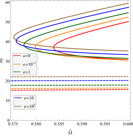
Figure 1: Dependence of the rescaled energy $\tilde{E}=g^{2}m_{V}^{-1}E$ on the parameter $\tilde{\Omega}=m_{V}^{-1}\Omega=-j_{\infty}$ for different values of the parameter $\kappa=g^{-2}\lambda$. The solid lines correspond to the modified dyons, and the dashed lines correspond to the Julia-Zee dyons.

Figure 1 presents the dependence of the energy $\tilde{E}$ for the modified dyon solution of model (1) on the parameter $\tilde{\Omega}$ for different values of the parameter $\kappa=g^{-2}\lambda$. In addition, Fig. 1 shows similar dependencies for the Julia-Zee dyon. Firstly, we see that the modified dyon solution exists only in a narrow range $\bigl{[}\tilde{\Omega}_{\min},2\tilde{M}\bigr{]}$ of values of the parameter $\tilde{\Omega}$. The right boundary of the interval $\bigl{[}\tilde{\Omega}_{\min},2\tilde{M}\bigr{]}$ is in agreement with Eq. (19), while the left boundary decreases monotonically with an increase in $\kappa$ and tends to a finite limit as $\kappa\rightarrow\infty$. The width of this interval is quite small and is only $0.02-0.025$, whereas the Julia-Zee dyon exists in a much wider wide interval $\left[0,1\right]$ of $|\tilde{\Omega}|$.

It follows from Fig. 1 that the $\tilde{E}(\tilde{\Omega})$ curves for the modified and Julia-Zee dyons behave completely differently. Indeed, we see that for the modified dyon, the $\tilde{E}(\tilde{\Omega})$ curves consist of two (lower and upper) branches that join at $\tilde{\Omega}=\tilde{\Omega}_{\min}$. For a given $\kappa$, the energy of the modified dyon reaches a minimum (maximum) value on the lower (upper) branch at the maximum value of $\tilde{\Omega}=2\tilde{M}$. Such a behaviour of the $\tilde{E}(\tilde{\Omega})$ curves is similar to their behaviour for an electrically charged Q-ball and completely different from that for the Julia-Zee dyon. Note that in Fig. 1, the $\tilde{E}(\tilde{\Omega})$ curves corresponding to the Julia-Zee dyon are practically indistinguishable from straight lines. This is because in Fig. 1, the width of the interval of $\tilde{\Omega}$ is much less than unity.

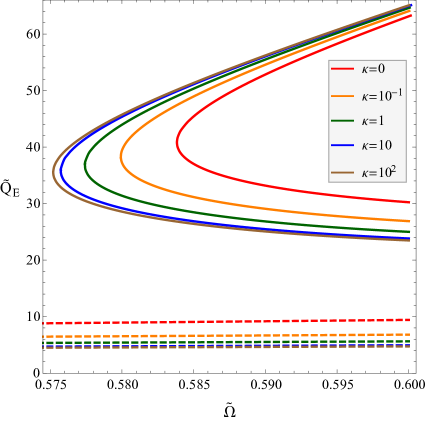
Figure 2: Dependence of the rescaled electric charge $\tilde{Q}_{E}=gQ_{E}$ on the parameter $\tilde{\Omega}=m_{V}^{-1}\Omega=-j_{\infty}$ for different values of the parameter $\kappa=g^{-2}\lambda$. The solid lines correspond to the modified dyons, and the dashed lines correspond to the Julia-Zee dyons.

Figure 2 presents the dependence of the electric charge $\tilde{Q}_{E}$ of the modified dyon solution on $\tilde{\Omega}$ for different values of $\kappa$. We see that the behavior of the $\tilde{Q}_{E}(\tilde{\Omega})$ curves is similar to that of the $\tilde{E}(\tilde{\Omega})$ curves for both the modified and Julia-Zee dyon solutions. The difference is that for the modified dyon solution, the $\tilde{E}(\tilde{\Omega})$ curves intersect each other, whereas the $\tilde{Q}_{E}(\tilde{\Omega})$ curves do not. As a result, for the modified dyon solution, the minimum and maximum energies are reached at $\tilde{\Omega}=2\tilde{M}$, and both of them increase with an increase in $\kappa$. But the minimum (maximum) electric charge of the modified dyon solution decreases (increases) with an increase in $\kappa$.

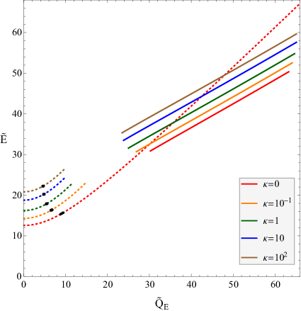
Figure 3: The $\tilde{E}(\tilde{Q}_{E})$ dependences for different $\kappa$. The solid lines correspond to the modified dyons, and the dotted lines correspond to the Julia-Zee dyons. The black segments on the dotted curves correspond to the ranges of the Julia-Zee dyon solutions presented in Figs. 1 and 2.

Figure 3 shows the dependences of the energy $\tilde{E}$ on the electric charge $\tilde{Q}_{E}$ for both the modified and Julia-Zee dyons. Note that in accordance with [16], the energy $\tilde{E}$ and the electric charge $\tilde{Q}_{E}$ of the Julia-Zee dyon can take arbitrarily large values only when $\kappa=0$ (the BPS case), whereas there are maximum possible values for both $\tilde{E}$ and $\tilde{Q}_{E}$ when $\kappa>0$. We see that the $\tilde{E}(\tilde{Q}_{E})$ curves are substantially different for the modified and Julia-Zee dyons. Firstly, except for the case $\kappa=0$, the energies and electric charges of the modified dyon solutions exceed the maximum possible values of the corresponding Julia-Zee dyon solutions. Secondly, for the modified dyon solutions, the curves $\tilde{E}(\tilde{Q}_{E})$ are visually indistinguishable from straight lines, which is not the case for the Julia-Zee dyon solutions. This is because in Figs. 1 and 2, the interval of variation of $\tilde{\Omega}$ is much less than $\tilde{\Omega}$ itself: $\Delta\tilde{\Omega}/\tilde{\Omega}\sim 1/30$, and the above property of the solid curves in Fig. 3 follows from Eq. (35) rewritten as

$$d\tilde{E}/d\tilde{Q}_{E}=\tilde{\Omega}.$$ (37)

Thirdly, unlike the Julia-Zee dyon, the energy and electric charge of the modified dyon cannot be arbitrarily large even when the parameter $\kappa=0$.

Figure 3 allows us to address the subject of stability of the modified dyon solution. Consider the family of the half-lines $a+b\tilde{Q}_{E}$ coming from the points of the dotted curve that correspond to a given value of $\kappa$. It is understood that the parameter $a$ depends on the origin point of the half-line. Then, it follows from Fig. 3 that for all the points $p$ of the dotted curves, the half-lines $a(p)+\tilde{Q}_{E}$ pass over the corresponding solid lines. Hence, the modified dyon is stable to the transition into the Julia-Zee dyon accompanied by emission of the charged vector bosons of mass $m_{V}=gv$. In contrast, for all the points $p$ of the dotted curves corresponding to $\kappa\geq 0.1$, the half-lines $a(p)+2\tilde{M}\tilde{Q}_{E}$ pass under the corresponding solid lines, where the appearance of the factor $2$ is due to the fact that the electric charges of the components of the scalar isodublet $\Phi$ are $\pm g/2$. The same is true for points $p$ of the dotted curve corresponding to $\kappa=0$ provided that $\tilde{Q}_{E}\left(p\right)\lesssim 25$. It follows that the modified dyon is unstable to the transition into the Julia-Zee dyon accompanied by emission of the charged scalar bosons of mass $M$.

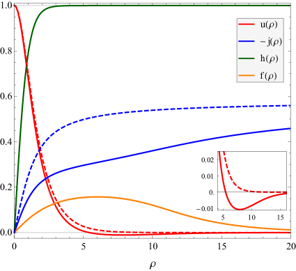
Figure 4: Ansatz functions of the dyon solutions corresponding to the parameters $\tilde{\Omega}=-j_{\infty}=0.58$ and $\kappa=g^{-2}\lambda=2$. The solid lines correspond to the modified dyon solution, and the dashed lines correspond to the Julia-Zee dyon solution.

The two possibilities described above are idealised. In reality, the transition of the modified dyon into the Julia-Zee dyon is accompanied by the emission of both vector and scalar bosons. Calculations show that the modified dyon is stable to the transition into the Julia-Zee dyon if the fraction of electric charge carried by the charged vector bosons exceeds $0.33$ for $\kappa=0$, and $0.24$ for $\kappa=100$.

In Fig. 4, we can see the ansatz functions corresponding to the two types of dyon solutions. The most significant differences are observed for $j(\rho)$. According to Eq. (24), the large $\rho$ asymptotics of this ansatz function is determined by the electric charge of the dyon. From Fig. 4, it follows that for a given $\tilde{\Omega}$ and $\kappa$, the electric charge of the modified dyon is substantially larger than that of the Julia-Zee dyon.

The ansatz function $u(\rho)$ is also different for the two dyon solutions, although not as much as $j(\rho)$. Nevertheless, there is an important difference between the two dyon solutions. From the subplot in Fig. 4, it follows that for the modified dyon, $u(\rho)$ crosses zero from above at finite $\rho$, reaches a minimum, and then tends to zero from below. At the same time, for the Julia-Zee dyon, $u(\rho)$ does not cross zero at finite $\rho$, but tends monotonically to zero from above. In contrast to $j(\rho)$ and $u(\rho)$, the ansatz function $h(\rho)$ is practically the same for the two dyon solutions.

From Fig. 4, we see that the maximum of the ansatz function $f(\rho)$ is outside of the core of the Julia-Zee dyon. Hence, the modified dyon consists of a core (deformed Julia-Zee dyon) surrounded by a spherical cloud of the charged scalar condensate. Note that in contrast to the electrically charged Q-ball, the density of the scalar condensate vanishes at the center of the modified dyon, which is caused by the boundary condition (18d).

5 Conclusion

We have shown that a modified dyon solution exists in a non-Abelian gauge model, which is essentially a modified Georgi-Glashow model. The modification consists in the inclusion of a self-interacting scalar isospinor field in the Lagrangian. The sixth-order self-interaction potential of the scalar field is of the Q-ball type. This modification of the Georgi-Glashow model leads to the existence of modified dyon solutions in addition to the usual Julia-Zee dyon solutions. The modified dyons exist in a much narrower parametric domain compared to the Julia-Zee dyons, and their properties differ significantly.

Firstly, except for the case $\kappa=0$, the energy and electric charge of the modified dyons significantly exceed those of the Julia-Zee dyons. Secondly, there is a non-zero minimum possible value of the electric charge for the modified dyon, whereas this is equal to zero for the Julia-Zee dyon. And thirdly, both the minimum and maximum value of the energy (electric charge) of the modified dyon are achieved at the maximum value of the parameter $\Omega$, whereas the energy (electric charge) of the Julia-Zee dyon increases monotonically with $\Omega$. As for the solutions themselves, the greatest differences are observed for the ansatz function $j(\rho)$, whose derivative determines the electric field strength of the dyon.

Finally, we note that various cosmological models tell us that the evolution of the early Universe proceeded through a sequence of phase transitions. Both electrically charged magnetic monopoles (dyons) and clouds of a charged scalar condensate can arise as a result of these phase transitions. The interaction of a long-range electric field of the dyon with the charged scalar condensate can lead to the formation of modified dyons similar to those considered in this paper.

References

- [1] S. K. Paul, A. Khare, Phys. Lett. B 174 (1986) 420. doi:10.1016/0370-2693(86)91028-2.
- [2] A. Khare, S. Rao, Phys. Lett. B 227 (1989) 424. doi:10.1016/0370-2693(89)90954-4.
- [3] J. Hong, Y. Kim, P. Y. Pac, Phys. Rev. Lett. 64 (1990) 2230. doi:10.1103/PhysRevLett.64.2230.
- [4] R. Jackiw, E. J. Weinberg, Phys. Rev. Lett. 64 (1990) 2234. doi:10.1103/PhysRevLett.64.2234.
- [5] R. Jackiw, K. Lee, E. J. Weinberg, Phys. Rev. D 42 (1990) 3488. doi:10.1103/PhysRevD.42.3488.
- [6] D. Bazeia, G. Lozano, Phys. Rev. D 44 (1991) 3348. doi:10.1103/PhysRevD.44.3348.
- [7] B. M. A. G. Piette, D. H. Tchrakian, W. J. Zakrzewski, Phys. Lett. B 339 (1994) 95. doi:10.1016/0370-2693(94)91139-8.
- [8] P. K. Ghosh, S. K. Ghosh, Phys. Lett. B 366 (1996) 199. doi:10.1016/0370-2693(95)01365-2.
- [9] K. Arthur, D. H. Tchrakian, Y. Yang, Phys. Rev. D 54 (1996) 5245. doi:10.1103/PhysRevD.54.5245.
- [10] M. Deshaies-Jacques, R. MacKenzie, Phys. Rev. D 74 (2006) 025006. doi:10.1103/PhysRevD.74.025006.
- [11] A. Yu. Loginov, JETP 118 (2014) 217. doi:10.1134/S1063776114020150.
- [12] F. Navarro-Lérida, E. Radu, D. H. Tchrakian, Phys. Rev. D 95 (2017) 085016. doi:10.1103/PhysRevD.95.085016.
- [13] B. Julia, A. Zee, Phys. Rev. D 11 (1975) 2227. doi:10.1103/PhysRevD.11.2227.
- [14] M. K. Prasad, C. M. Sommerfield, Phys. Rev. Lett. 35 (1975) 760. doi:10.1103/PhysRevLett.35.760.
- [15] S. Coleman, S. J. Parke, A. Neveu, C. M. Sommerfield, Phys. Rev. D 15 (1977) 544. doi:10.1103/PhysRevD.15.544.
- [16] Y. Brihaye, B. Kleihaus, D. H. Tchrakian, J. Math. Phys. 40 (1999) 1136. doi:10.1063/1.532793.
- [17] E. Radu, D. H. Tchrakian, Phys. Lett. B 632 (2006) 109. doi:10.1016/j.physletb.2005.10.020.
- [18] K. Lee, J. A. Stein-Schabes, R. Watkins, L. M. Widrow, Phys. Rev. D 39 (1989) 1665. doi:10.1103/PhysRevD.39.1665.
- [19] C. H. Lee, S. U.Yoon, Mod. Phys. Lett. A 6 (1991) 1479. doi:10.1142/S0217732391001597.
- [20] H. Arodz, J. Lis, Phys. Rev. D 79 (2009) 045002. doi:10.1103/PhysRevD.79.045002.
- [21] T. Tamaki, N. Sakai, Phys. Rev. D 90 (2014) 085022. doi:10.1103/PhysRevD.90.085022.
- [22] Y. Brihaye, V. Diemer, B. Hartmann, Phys. Rev. D 89 (2014) 084048. doi:10.1103/PhysRevD.89.084048.
- [23] I. E. Gulamov, E. Y. Nugaev, M. N. Smolyakov, Phys. Rev. D 89 (2014) 085006. doi:10.1103/PhysRevD.89.085006.
- [24] I. E. Gulamov, E. Y. Nugaev, A. G. Panin, M. N. Smolyakov, Phys. Rev. D 92 (2015) 045011. doi:10.1103/PhysRevD.92.045011.
- [25] V. Loiko, Ya. Shnir, Phys. Lett. B 797 (2019) 134810. doi:10.1016/j.physletb.2019.134810.
- [26] A. Yu. Loginov, V. V. Gauzshtein, Phys. Rev. D 102 (2020) 025010. doi:10.1103/PhysRevD.102.025010.
- [27] R. Jackiw, S. Templeton, Phys. Rev. D 23 (1981) 2291. doi:10.1103/PhysRevD.23.2291.
- [28] J. F. Schonfeld, Nucl. Phys. B 185 (1981) 157. doi:10.1016/0550-3213(81)90369-2.
- [29] S. Deser, R. Jackiw, S. Templeton, Phys. Rev. Lett. 48 (1982) 975. doi:10.1103/PhysRevLett.48.975.
- [30] S. Coleman, Nucl. Phys. B 262 (1985) 263.
- [31] T. D. Lee, Y. Pang, Phys. Rep. 221 (1992) 251.
- [32] R. Friedberg, T. D. Lee, A. Sirlin, Phys. Rev. D 13 (1976) 2739. doi:10.1103/PhysRevD.13.2739.
- [33] R. Friedberg, T. D. Lee, A. Sirlin, Nucl. Phys. B 115 (1976) 1. doi:10.1016/0550-3213(76)90274-1.
- [34] R. Friedberg, T. D. Lee, A. Sirlin, Nucl. Phys. B 115 (1976) 32. doi:10.1016/0550-3213(76)90275-3.
- [35] N. Manton, P. Sutclffe, Topological Solitons, Cambridge University Press, Cambridge, 2004.
- [36] H. Georgi, S. L. Glashow, Phys. Rev. D 6 (1972) 2977. doi:10.1103/PhysRevD.6.2977.
- [37] A. Yu. Loginov, Phys. Lett. B 822 (2021) 136662. doi:10.1016/j.physletb.2021.136662.
- [38] A. Yu. Loginov, Phys. Lett. B 777 (2018) 340. doi:10.1016/j.physletb.2017.12.054.
- [39] A. Yu. Loginov, V. V. Gauzshtein, Phys. Lett. B 784 (2018) 112. doi:10.1016/j.physletb.2018.07.044.
- [40] G. ’t Hooft, Nucl. Phys. B 79 (1974) 276. doi:10.1016/0550-3213(74)90486-6.
- [41] A. M. Polyakov, JETP Lett. 20 (1974) 194.
- [42] F. R. Klinkhamer, N. S. Manton, Phys. Rev. D 30 (1984) 2212. doi:10.1103/PhysRevD.30.2212.
- [43] P. Goddard, D. I. Olive, Rep. Prog. Phys. 41 (1978) 1357. doi:10.1088/0034-4885/41/9/001.
- [44] Maple 2022.1. Maplesoft, a division of Waterloo Maple Inc., Waterloo, Ontario.