Upper limit on axion-photon coupling from Markarian 421
††preprint: ITP-24-070, BNU-24-039The pseudo-Nambu-Goldstone boson (pNGB), axions, are motivated candidates for physics beyond the Standard Model (SM). The QCD axion Peccei and Quinn (1977a, b) was originally postulated to solve the strong CP problem, meanwhile, it is the cold dark matter (DM) candidate. Additionally, the axionlike particle (ALP) can also account for the DM, but is not associated to the solution of the strong CP problem. For simplicity, in the following the “axion” stands for the ALP. The axion-photon interaction has a two-photon vertex
| (1) |
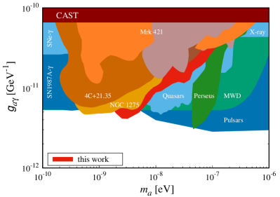
where is the axion field, is the axion-photon coupling constant, is the electromagnetic field tensor and its dual tensor . Considering the interaction between the axion and very high energy (VHE) photon in the astrophysical magnetic fields, it can lead to some detectable effects, such as the reduced TeV opacity of the Universe Mirizzi et al. (2007); Hooper and Serpico (2007); Ajello et al. (2016). The VHE TeV gamma-ray emissions from the extragalactic space, such as the active galactic nuclei (AGN), are mainly affected by the effect of extragalactic background light (EBL) absorption through the electron-positron pair production process . If considering the axion-photon conversion and further back-conversion in several astrophysical magnetic fields, the EBL absorption effect can be reduced and the Universe would appear to be more transparent than expected based on the pure EBL absorption. Meanwhile, it also provides a natural mechanism to constrain the axion properties with the axion mass and the coupling . See Fig. 1 for the latest axion-photon limits in the plane.
In this letter, we obtain a stringent upper limit on axion-photon coupling from the TeV blazar Markarian 421 with the 1038 days VHE gamma-ray observations. The source Markarian 421 (, , J2000) is a well-known nearby blazar at a redshift , it also known as other names, Mrk 421, TeV J1104+382, and 1ES 1101+384. Markarian 421 belongs to a subclass of AGNs, the high-frequency peaked BL Lac (HBL) or the high-synchrotron peaked BL Lac (HSP) object, which are classified by the weak or missing broad emission lines in the optical spectra. It was first discovered with the VHE emission by the Whipple 10-m Observatory Punch et al. (1992). Many works were investigated to constrain the axion-photon coupling from the gamma-ray of Markarian 421 Li et al. (2021); Gao et al. (2024). Recently, its long-term gamma-ray spectra are measured by the collaborations, the Large Area Telescope on board NASA’s Fermi Gamma-ray Space Telescope (Fermi-LAT) and the High Altitude Water Cherenkov (HAWC) Gamma-Ray Observatory, with the 1038 days of exposure from 2015 June to 2018 July Albert et al. (2022). Using this long-term gamma-ray flux, we consider the axion-photon conversion effect on the spectral energy distributions (SEDs) and set the limit on axion-photon coupling.
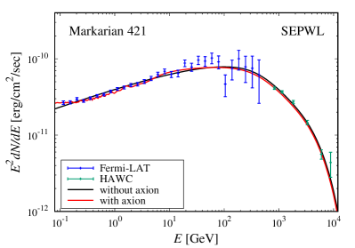
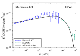
We first show the long-term VHE gamma-ray observations of Markarian 421 under the null hypothesis. The experimental data of Markarian 421 measured by Fermi-LAT and HAWC are shown in Fig. 2. To fit the gamma-ray spectrum, the intrinsic spectral model is selected as the power law with a super-exponential cut-off (SEPWL), , where represents the VHE photon energy, is a normalized constant, is the spectral index, , , and are free parameters, and we fix . As mentioned before, the main effect on VHE photon in the extragalactic space is the EBL photon absorption effect with an absorption factor , where is the optical depth, and the EBL spectral model is taken as Franceschini-08 Franceschini et al. (2008). Then we have the chi-square value under the null hypothesis , where (Fermi-LAT: 30, and HAWC: 6) represents the gamma-ray spectral point number, and represent the detected flux and its uncertainty, respectively. Note that here the gamma-ray intrinsic spectral model is selected with the minimum best-fit reduced from several common spectral models, see the Supplemental Material. We show the best-fit gamma-ray SED of Markarian 421 in Fig. 2. The black line represents the best-fit SED under the null hypothesis with and , where is the degree of freedom.
Next, we consider the effects of axion-photon conversion on VHE gamma-ray propagations from the source Markarian 421 to the Earth. In the transverse homogeneous magnetic field, the axion-photon conversion probability can be simply characterized as , where is the transverse magnetic field, is the oscillation length, and is the direction of the axion-photon propagation. While in the non-homogeneous astrophysical magnetic field, the magnetic field can be modeled as the domain-like structure and each domain can be regarded as homogeneous. In this case, the final photon-axion-photon conversion probability (the final photon survival probability) can be described in the density matrix formal , where represents the propagation distance, represents the whole transfer matrix, and represent the initial and final axion-photon density matrices, respectively, and . In this work, the axion-photon propagation process from Markarian 421 to the Earth can be divided into three parts, the blazar jet magnetic field, the extragalactic space, and the magnetic field in the Milky Way. We first discuss the axion-photon conversion in the blazar jet magnetic field of Markarian 421, which can be described by the poloidal and toroidal components. Here we consider a transverse magnetic field model with an electron density model , where corresponds to the distance from the source central black hole to the VHE emission region, represents the radius of the VHE emission region, represents the angle between the jet axis and the line of sight, and correspond to the core magnetic field and electron density at , respectively. We also consider the energy transformation between the laboratory and co-moving frames, and , with the Doppler factor . For Markarian 421, we take , , , , , and Albert et al. (2022). Note that for the jet region at , the magnetic field is wake and can be taken as zero. Then for the host galaxy region of Markarian 421, we neglect the axion-photon conversion in this part. Secondly, in the extragalactic space, we just consider the EBL absorption effect on VHE photon through the pair-production process. Since the magnetic field strength in this region is small , the axion-photon conversion effect will be weak and can be neglected. Thirdly, in the magnetic field of the Milky Way, we consider the axion-photon conversion again. Here the Galactic magnetic field is simulated with the disk and halo components, and also the “X-field” component at the Galactic center Jansson and Farrar (2012a, b).
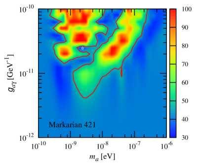
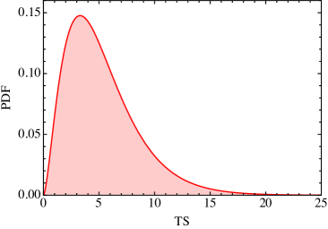
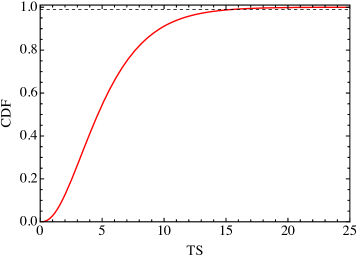
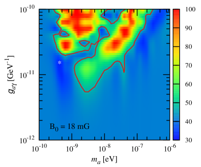
Using the final photon survival probability discussed above, now we can obtain the chi-square value under the axion hypothesis . For one axion parameter set, we can derive the best-fit chi-square , and also the best-fit chi-square distribution in the parameter plane. In Fig. 3, we show the best-fit chi-square distribution for Markarian 421 in the plane, where the label “” represents the minimum best-fit chi-square at . Meanwhile, we also show the best-fit gamma-ray SED corresponding to in Fig. 2 with the red line. Compared with the null hypothesis (black line), the minimum best-fit chi-square under the axion hypothesis can be significantly depressed. Using the best-fit chi-square distribution, here we set the 99% confidence level () limit on axion-photon coupling. In order to obtain the value of the threshold chi-square , 400 sets of the VHE gamma-ray observations of Markarian 421 in the pseudo-experiments by Gaussian samplings are simulated to derive the distribution of the test statistic (TS), , where and are the best-fit chi-squares of the null and axion hypotheses in the Monte Carlo simulations, respectively. It obeys the non-central chi-square distribution with the non-centrality and the effective , and we use it to derive the 99% chi-square difference . Then the 99% threshold chi-square is given by . In our simulations, we have the non-centrality and the effective , indicating the threshold chi-square (see the Supplemental Material). Then we show in Fig. 3 the 99% limit with the red contours, the region in the contour is excluded. Finally, we have the 99% upper limit on axion-photon coupling set by Markarian 421 with the 1038 days VHE gamma-ray observations measured by Fermi-LAT and HAWC, which is constrained to the coupling constant
| (2) |
for the axion mass
| (3) |
Compared with the latest axion-photon limits in the plane, see also Fig. 1 with the red contour, it is the most stringent upper limit in this mass region. In addition, we also have an upper limit for the axion mass .
In summary, we have obtained a stringent upper limit on axion-photon coupling from the 1038 days gamma-ray observations of the TeV blazar Markarian 421. The long-term VHE gamma-ray spectra are measured by the collaborations Fermi-LAT and HAWC from 2015 June to 2018 July. We show the best-fit SEDs of Markarian 421 under the null and axion hypotheses. Then we set the axion-photon limit in the plane. The 99% upper limit set by Markarian 421 is for the axion mass . It is the most stringent upper limit in this axion mass region. Additionally, since the VHE gamma-ray observations of another TeV blazar Markarian 501 (with redshift ) at the same time are given in Ref. Albert et al. (2022), we also make the axion analysis for this source in the Supplemental Material but no stringent limits are obtained. See also the Supplemental Material for more details in the calculations.
Acknowledgments.—We thank Sara Coutio de Len for providing the experimental data of Fermi-LAT and HAWC. This work was supported by the National Key R&D Program of China (Grant No. 2017YFA0402204), the CAS Project for Young Scientists in Basic Research YSBR-006, and the National Natural Science Foundation of China (NSFC) (Grants No. 11775025, No. 11821505, No. 11825506, No. 12047503, and No. 12175027).
References
- Peccei and Quinn (1977a) R. Peccei and H. R. Quinn, Phys. Rev. D 16, 1791 (1977a).
- Peccei and Quinn (1977b) R. Peccei and H. R. Quinn, Phys. Rev. Lett. 38, 1440 (1977b).
- Mirizzi et al. (2007) A. Mirizzi, G. G. Raffelt, and P. D. Serpico, Phys. Rev. D 76, 023001 (2007), arXiv:0704.3044 [astro-ph] .
- Hooper and Serpico (2007) D. Hooper and P. D. Serpico, Phys. Rev. Lett. 99, 231102 (2007), arXiv:0706.3203 [hep-ph] .
- Ajello et al. (2016) M. Ajello et al. (Fermi-LAT), Phys. Rev. Lett. 116, 161101 (2016), arXiv:1603.06978 [astro-ph.HE] .
- O’HARE (2020) C. O’HARE, “cajohare/axionlimits: Axionlimits,” (2020).
- Punch et al. (1992) M. Punch et al., Nature 358, 477 (1992).
- Li et al. (2021) H.-J. Li, J.-G. Guo, X.-J. Bi, S.-J. Lin, and P.-F. Yin, Phys. Rev. D 103, 083003 (2021), arXiv:2008.09464 [astro-ph.HE] .
- Gao et al. (2024) L.-Q. Gao, X.-J. Bi, J.-G. Guo, W. Lin, and P.-F. Yin, Phys. Rev. D 109, 063003 (2024), arXiv:2309.02166 [astro-ph.HE] .
- Albert et al. (2022) A. Albert et al. (HAWC), Astrophys. J. 929, 125 (2022), arXiv:2106.03946 [astro-ph.HE] .
- Franceschini et al. (2008) A. Franceschini, G. Rodighiero, and M. Vaccari, Astron. Astrophys. 487, 837 (2008), arXiv:0805.1841 [astro-ph] .
- Jansson and Farrar (2012a) R. Jansson and G. R. Farrar, Astrophys. J. 757, 14 (2012a), arXiv:1204.3662 [astro-ph.GA] .
- Jansson and Farrar (2012b) R. Jansson and G. R. Farrar, Astrophys. J. Lett. 761, L11 (2012b), arXiv:1210.7820 [astro-ph.GA] .
Upper limit on axion-photon coupling from Markarian 421
Supplemental Material
Hai-Jun Li, Wei Chao, and Yu-Feng Zhou
This is not the first investigation to constrain the axion-photon coupling from the TeV blazar Markarian 421. In Ref. Li et al. (2021), they first investigated the axion-photon conversion effect from this source by using the 4.5 years gamma-ray data of Fermi-LAT and Astrophysical Radiation with Ground-based Observatory at YangBaJing (ARGO-YBJ), showing the upper limit for the axion mass . In Ref. Gao et al. (2024), they presented the axion limits from Markarian 421 by using the 1 year data of Fermi-LAT and Major Atmospheric Gamma Imaging Cherenkov Telescopes (MAGIC), showing the similar upper limits but for the axion mass . While in this work, we obtain a more stringent upper limit from the VHE gamma-ray data of Fermi-LAT and HAWC, which is even the most stringent limit compared with other astrophysical results in the axion mass . This is mainly because the large value of obtained in this work. We know that here the greatest impact on the final result are parameters and , both larger of them will lead to more stringent limit. We also discuss the impact of the parameter uncertainty of in the Supplemental Material. On the other hand, compared with the experimental data of ARGO-YBJ and MAGIC, the data of HAWC shows smaller uncertainty in the high energy region.
An interesting point in this work is the minimum best-fit chi-square at , we also note that the small chi-square in this region in other works Li et al. (2021), especially in Ref. Ajello et al. (2016) with the NGC 1275 observations set by Fermi-LAT. It is still unclear whether there are any new interpretations for this parameter region.
This Supplemental Material is organized as follows. In Sec. I, we show the gamma-ray SEDs of Markarian 421 under the null hypothesis. In Sec. II, we display the final photon survival probability. In Sec. III, we show the TS distribution. In Sec. IV, we discuss the impact of the parameter uncertainty. Then we make the axion analysis for the source Markarian 501 in Sec. V. Finally, we attach the experimental gamma-ray data of Markarian 421 and Markarian 501 in Sec. VI.
I SEDs under the null hypothesis
In this section, we show the gamma-ray SEDs of Markarian 421 under the null hypothesis with the different intrinsic spectral models. It can be described by the simple and smooth concave functions with three to five free parameters. We take the common spectral models as the power law with exponential cut-off (EPWL, with three parameters), the power law with super-exponential cut-off (SEPWL, with four parameters), the log-parabola (LP, with four parameters), and the log-parabola with exponential cut-off (ELP, with five parameters),
| (S1) | |||||
| (S2) | |||||
| (S3) | |||||
| (S4) |
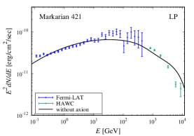
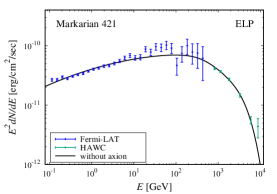
where , , , , , and are free parameters. While for the models EPWL and SEPWL, we fix . Using these intrinsic spectral models, we fit the gamma-ray of Markarian 421 and list the corresponding best-fit chi-squares in Table 1. Due to the smallest value of for SEPWL, we finally select this spectral model to fit Markarian 421. The best-fit SEDs for other spectral models are also shown in Fig. S1.
II Final photon survival probability
In the transverse homogeneous magnetic field , the axion-photon conversion probability can be described by with the oscillation length
| (S5) |
where is the plasma frequency, is the axion/photon energy, is the fine-structure constant, is the critical magnetic field, and represents the cosmic microwave background (CMB) photon dispersion effect.
| Model | parameter number | ||
|---|---|---|---|
| EPWL | 3 | 158.97 | 4.82 |
| SEPWL | 4 | 44.24 | 1.38 |
| LP | 4 | 244.52 | 7.64 |
| ELP | 5 | 63.25 | 2.04 |
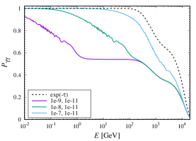
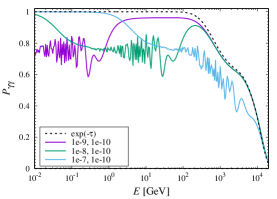
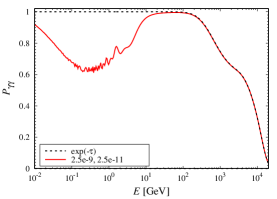
Here we show in Fig. S2 the final photon survival probability for Markarian 421. In the left and middle panels, we show for several typical axion-photon coupling parameter sets. In addition, we also show in the right panel the final photon survival probability for the minimum best-fit chi-square in the plane, with .
III TS distribution
We also show the test statistic (TS) distribution in Fig. S3 with the probability density function (PDF) and cumulative distribution function (CDF). In our simulations, we have the non-centrality and the effective , indicating the 99% chi-square difference , and the threshold chi-square . Then we use this value to set the 99% limit in the axion parameter plane.
IV Impact of the parameter uncertainty
Since we take the Markarian 421 blazar jet core magnetic field at as , here we discuss the impact of the uncertainty of . Ws show in Fig. S4 the best-fit chi-square distribution in the plane with different values of . Compared with , the 99% axion-photon limits are also shown in Fig. S5 with different lines. As we expected, the larger leads to the more stringent limit. The parameter has a similar impact on the final result. In addition, since we take and it has little impact on the limit, here we do not show the impact of the uncertainty of .
V Axion analysis for Markarian 501
Additionally, since the VHE gamma-ray observations of another TeV blazar Markarian 501 (Mrk 501, with redshift ) at the same time are also measured by Fermi-LAT and HAWC, in the following we make the axion analysis for this source. The experimental data of Fermi-LAT (27 points) and HAWC (6 points) are shown in Fig. S6. Here we also select the gamma-ray intrinsic spectral model SEPWL to fit Markarian 501, and the best-fit SED corresponds to is shown in Fig. S6. The best-fit chi-squares for other spectral models are listed in Table 2.
| Model | parameter number | ||
|---|---|---|---|
| EPWL | 3 | 74.91 | 2.50 |
| SEPWL | 4 | 42.06 | 1.45 |
| LP | 4 | 53.61 | 1.85 |
| ELP | 5 | 50.68 | 1.81 |
For the blazar jet magnetic field of Markarian 501, we take , , , , , and . Then we obtain the best-fit chi-square distribution in the plane, which is shown in Fig. S7. The value of the minimum best-fit chi-square in the plane is at , see also the corresponding SED in Fig. S6. In our TS analysis, we have the non-centrality and the effective , indicating the 99% threshold chi-square , corresponding to the red contour in Fig. S7. Since it shows a weak limit, we also show the 95% limit () with the orange contour. While for Markarian 421, since the value of is smaller than the best-fit chi-square under the null hypothesis , we just show the 99% limit. In summary, here we do not obtain a stringent upper limit from the source Markarian 501.
VI Experimental gamma-ray data
Finally, we attach the experimental gamma-ray data of Markarian 421 and Markarian 501 measured by Fermi-LAT and HAWC in Table 3 and 4, respectively.
| Collaboration | (GeV) | () | () |
|---|---|---|---|
| Fermi-LAT | 0.1152 | 2.662e-11 | 1.457e-12 |
| Fermi-LAT | 0.1531 | 2.686e-11 | 1.297e-12 |
| Fermi-LAT | 0.2034 | 2.984e-11 | 1.220e-12 |
| Fermi-LAT | 0.2701 | 2.805e-11 | 1.186e-12 |
| Fermi-LAT | 0.3588 | 3.059e-11 | 1.204e-12 |
| Fermi-LAT | 0.4766 | 3.268e-11 | 1.247e-12 |
| Fermi-LAT | 0.633 | 3.405e-11 | 1.324e-12 |
| Fermi-LAT | 0.8409 | 3.733e-11 | 1.472e-12 |
| Fermi-LAT | 1.117 | 4.030e-11 | 1.667e-12 |
| Fermi-LAT | 1.484 | 4.214e-11 | 1.852e-12 |
| Fermi-LAT | 1.971 | 4.542e-11 | 2.143e-12 |
| Fermi-LAT | 2.618 | 4.647e-11 | 2.466e-12 |
| Fermi-LAT | 3.477 | 5.040e-11 | 2.922e-12 |
| Fermi-LAT | 4.619 | 5.540e-11 | 3.508e-12 |
| Fermi-LAT | 6.135 | 6.246e-11 | 4.246e-12 |
| Fermi-LAT | 8.15 | 6.849e-11 | 5.077e-12 |
| Fermi-LAT | 10.82 | 6.250e-11 | 5.583e-12 |
| Fermi-LAT | 14.38 | 6.444e-11 | 6.508e-12 |
| Fermi-LAT | 19.1 | 8.767e-11 | 8.731e-12 |
| Fermi-LAT | 25.37 | 7.798e-11 | 9.440e-12 |
| Fermi-LAT | 33.7 | 9.612e-11 | 1.198e-11 |
| Fermi-LAT | 44.76 | 9.335e-11 | 1.353e-11 |
| Fermi-LAT | 59.46 | 1.023e-10 | 1.630e-11 |
| Fermi-LAT | 78.98 | 9.133e-11 | 1.762e-11 |
| Fermi-LAT | 104.9 | 4.667e-11 | 1.477e-11 |
| Fermi-LAT | 139.4 | 7.443e-11 | 2.167e-11 |
| Fermi-LAT | 185.1 | 1.001e-10 | 2.888e-11 |
| Fermi-LAT | 245.9 | 7.840e-11 | 2.949e-11 |
| Fermi-LAT | 326.6 | 7.500e-11 | 3.342e-11 |
| Fermi-LAT | 433.8 | 6.148e-11 | 3.538e-11 |
| HAWC | 831.3 | 4.124e-11 | 1.474e-12 |
| HAWC | 1145 | 3.678e-11 | 1.371e-12 |
| HAWC | 1835 | 2.713e-11 | 1.323e-12 |
| HAWC | 3306 | 1.463e-11 | 9.799e-13 |
| HAWC | 5984 | 5.615e-12 | 7.881e-13 |
| HAWC | 8809 | 4.379e-12 | 1.578e-12 |
| Collaboration | (GeV) | () | () |
|---|---|---|---|
| Fermi-LAT | 0.1153 | 9.598e-12 | 1.459e-12 |
| Fermi-LAT | 0.1531 | 9.851e-12 | 1.259e-12 |
| Fermi-LAT | 0.2034 | 7.649e-12 | 1.041e-12 |
| Fermi-LAT | 0.2701 | 8.056e-12 | 9.441e-13 |
| Fermi-LAT | 0.3588 | 9.912e-12 | 9.147e-13 |
| Fermi-LAT | 0.4764 | 1.083e-11 | 8.899e-13 |
| Fermi-LAT | 0.6332 | 1.112e-11 | 8.724e-13 |
| Fermi-LAT | 0.8408 | 1.152e-11 | 9.082e-13 |
| Fermi-LAT | 1.117 | 1.256e-11 | 9.967e-13 |
| Fermi-LAT | 1.484 | 1.117e-11 | 1.039e-12 |
| Fermi-LAT | 1.971 | 1.319e-11 | 1.219e-12 |
| Fermi-LAT | 2.618 | 1.413e-11 | 1.436e-12 |
| Fermi-LAT | 3.477 | 1.513e-11 | 1.609e-12 |
| Fermi-LAT | 4.62 | 1.604e-11 | 1.935e-12 |
| Fermi-LAT | 6.137 | 1.662e-11 | 2.205e-12 |
| Fermi-LAT | 8.152 | 1.755e-11 | 2.624e-12 |
| Fermi-LAT | 10.82 | 2.217e-11 | 3.312e-12 |
| Fermi-LAT | 14.38 | 1.144e-11 | 2.829e-12 |
| Fermi-LAT | 19.1 | 2.516e-11 | 4.681e-12 |
| Fermi-LAT | 25.37 | 2.165e-11 | 4.962e-12 |
| Fermi-LAT | 33.7 | 2.281e-11 | 5.872e-12 |
| Fermi-LAT | 44.75 | 3.127e-11 | 7.846e-12 |
| Fermi-LAT | 59.47 | 2.949e-11 | 8.848e-12 |
| Fermi-LAT | 78.99 | 1.660e-11 | 7.688e-12 |
| Fermi-LAT | 104.9 | 2.801e-11 | 1.143e-11 |
| Fermi-LAT | 139.4 | 4.310e-11 | 1.626e-11 |
| Fermi-LAT | 185.1 | 4.946e-11 | 2.010e-11 |
| HAWC | 749.8 | 9.850e-12 | 1.318e-12 |
| HAWC | 1060 | 8.533e-12 | 1.155e-12 |
| HAWC | 1890 | 3.696e-12 | 8.000e-13 |
| HAWC | 3890 | 2.397e-12 | 5.134e-13 |
| HAWC | 7362 | 1.797e-12 | 3.769e-13 |
| HAWC | 10900 | 2.035e-12 | 7.075e-13 |