mystyle \setfoot[0][][]0
A Broadband 3-D Numerical FEM Study on the Characterization of
Dielectric Relaxation Processes in Soils111Proc. 10th International
Conference on Electromagnetic Wave Interaction with Water and Moist Substances,
ISEMA 2013, Editor: K. Kupfer,
Weimar, Germany, Sep 25-27, 142-151, 2013
Norman Wagner1, Markus Loewer2
1 Institute of Material Research and Testing at the Bauhaus-University Weimar, Germany
2 Leibniz Institute for Applied Geophysics (LIAG), Hannover, Germany
ABSTRACT
Soil as a complex multi-phase porous
material typical exhibits several distributed relaxation processes in the frequency range from 1 MHz to
approximately 10 GHz of interest in applications. To relate physico-chemical
material parameters to the dielectric relaxation behavior, measured dielectric
relaxation spectra have to be parameterized. In this context, a broadband numerical 3D FEM
study was carried out to analyze the possibilities and limitations in
the characterization of the relaxation processes in complex systems.
Keywords: soil matric potential, soil moisture, dielectric relaxation behavior of soil
1 INTRODUCTION
The dielectric relaxation behavior of porous media such as soils contains valuable information of the material due to a strong correlation with the volume fractions of the soil phases as well as contributions by interactions between the pore solution and mineral particles [1, 2]. Hence, high frequency electromagnetic remote sensing techniques offer the possibility to estimate physico-chemical parameters fast and non-invasive [3].
To relate physico-chemical material parameters to the dielectric relaxation behavior, measured dielectric spectra have to be parameterized. Soil as a multi-phase porous material typical exhibits different relaxation processes mostly with a distribution of relaxation times in the frequency range of interest in applications [2]. In this context, a broadband numerical 3D FEM study in combination with a global inversion approach was carried out to analyze the possibility and limitations for the characterization and parametrization of the relaxation behavior. To quantify the uncertainty in the estimation of relaxation parameters from a data-set of full two port scattering parameters in the frequency range from 1 MHz to 10 GHz known dielectric relaxation spectra of standard materials as well as soil-related spectra were used. The spectra were analyzed by means of a broadband generalize dielectric relaxation model (GDR, see [1]).
2 MODELING AND INVERSION
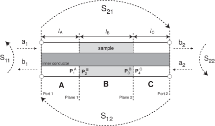
The structure used in the numerical 3D-FEM calculation of the full S-parameter set was based on a 50 coaxial transmission line cell introduced in [4] for determining HF-EM properties of undisturbed soil samples. The cell has an outer diameter of the inner conductor =16.9 mm, an inner diameter of the outer conductor =38.8 mm and a length =50 mm. The used input spectra are choosen according to (i) experimental results of de-ionized water, ethanol, methanol as well as water with defined electrical conductivity obtained with open ended coaxial line technique (see [5]) and (ii) different soil types with defined variation in dispersion and absorption as well as conductive losses (see [1, 4]). To study the accuracy in determination of relaxation parameters from a data-set of broadband full two port S-Parameters uni-, bi- and tri-modal dielectric relaxation spectra are used. In Table 1 the model parameters of the used materials are summarized.
2.1 3-D Finite Element Modeling
The numerical calculation was carried out based on a commercial software package for 3D-FEM simulation provided by Ansys (Ansoft HFSS). Ansoft HFSS solves Maxwell’s equations using a finite element method, in which the solution domain is divided into tetrahedral mesh elements. With tangential element basis functions field values from both nodal values at vertices and on edges are interpolated. Outer surface cross sections of the coaxial line structure corresponding to appropriate measurement planes were used as wave ports. A finite conductivity boundary condition was used at the outer surface in parallel to the length of the cell. The mesh generation was performed automatically with l/3 wavelength based adaptive mesh refinement at a solution frequency of 10 GHz. Broadband complex S-parameters were calculated based on an interpolating sweep (1 MHz - 10 GHz) with extrapolation to DC. The computed generalized S-matrix is normalized to 50 for comparison of the numerical calculated with measured S-parameters (see [6]).
| Material | ethanol | methanol | water | soil #1 | soil #2 | soil #3 |
| (sand-analog) | (silt-analog) | (clay-analog) | ||||
| 3.9 | 5.65 | 4.5 | 5 | 5 | 5 | |
| 20.7 | 28.0 | 75.2 | 30 | 30 | 30 | |
| [ps] | 160.7 | 56.4 | 9.8 | 1 | 1 | 1 |
| 1 | 1 | 1 | 1 | 1 | 1 | |
| - | - | - | - | |||
| [ns] | - | - | - | - | 10 | 10 |
| - | - | - | - | 1 | ||
| - | - | - | - | 0 | 0 | |
| - | - | - | - | - | 100 | |
| [s] | - | - | - | - | - | 10 |
| - | - | - | - | - | ||
| - | - | - | - | - | 0 | |
| [S/m] | 0 | 0 |
2.2 Quasi-analytical Inversion
In general, assuming propagation in TEM mode and non magnetic materials of a sample in a transmission line is related to its complex impedance or complex propagation factor as follows (see [7, 8, 9, 6]):
| (1) | |||||
| (2) | |||||
| (3) |
Herein is the characteristic impedance of the empty transmission line, the velocity of light with absolute dielectric permittivity, absolute magnetic permeability of vacuum, angular frequency and imaginary unit . To obtain or from measured complex S-parameters several quasi analytical approaches are available. In the transmission/reflection approach with coaxial transmission line technique, a sample is inserted into the coaxial line (see Fig. 1). The scattering equations corresponding to the experimental set-up or the implemented numerical model have to be found from an analysis of the electric field at the sample interfaces.
(i)
(ii)
In the modified NRW algorithm suggested by Baker-Jarvis et al. (see [8], hereafter called BJ) the following formulation of the appropriate scattering parameters is used:
| (6) |
with length of the empty coaxial line cell between the calibration planes and length of the coaxial line section filled with the sample. Than and reads:
| (7) |
The complex propagation factor and complex impedance are in both cases given as follows:
| (8) |
The results of equation (8) for the propagation factor are ambiguous due to the logarithm of the complex number with where the imaginary part is given by with . The correct as a function of frequency has to be numerically determined based on the discontinuity of . In this study we applied an one dimensional phase unwrapping procedure provided in matlab. Moreover, the correct roots in equation (5) or (7) were chosen such that , and , are satisfied.
(iii)
A further approach were suggested by Gorriti et al. [11] which is based on appropriate propagation matrixes ( with , see [12]):
| (9) |
In the numerical implemented structure section and have identical propagation properties and the material in the sample section is homogeneous and isotropic. The determination of the appropriate complex impedance or propagation factor of the sample from measured scattering parameters in the PM-approach is here developed in terms of and . The matrixes are given as follows:
| (10) |
with interface between section and as well as
| (11) |
Herein are the appropriate propagation factor and characteristic impedance of the -th section with sample section B labeled with . The dielectric relaxation spectrum of the material under study is contained within matrix B, which is given with equation (10) and (11) by
| (12) |
Equation (9) in terms of and can be rewritten
| (13) |
Substituting according to equation (12) into equation (13) and eliminating the exponential terms, the impedance of the sample than becomes
| (14) |
If the impedance terms are eliminated the propagation factor is given as
| (15) |
The correct sign were chosen such that and .
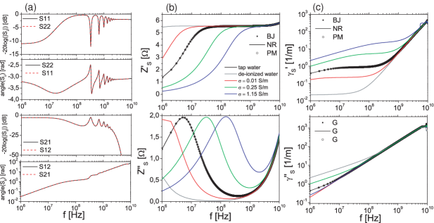
Hence, all three algorithms can be formulated in a way to determine explicitly and . For the calculation of the permittivity spectra the appropriate relationship according to equation (1), (2) or (3) can be used (see [13]). In Fig. 2 the results in case of tap water are shown. The numerical calculated complex S-parameters with the 3D-FEM approach subsequently were used to compute in the frequency range between 1 MHz to 10 GHz with the introduced quasi-analytical methods: classical NRW, BJ and the propagation matrix algorithm (PM).
2.3 Inverse Modeling
Soil as a multi-phase porous material typical exhibits several relaxation processes in the frequency range between 1 MHz and 10 GHz of interest in applications [3, 14, 1]. Dielectric loss spectra of saturated and unsaturated porous materials are the result of broadly distributed relaxation processes ([15, 16, 17, 18, 19, 20, 1, 5]). Based on the theory of fractional time evolutions Hilfer [21] derived relaxation functions for the complex frequency dependent dielectric permittivity of amorphous and glassy materials which are used to develop an generalized broadband relaxation model (GDR, see [20, 1]):
| (16) |
with high frequency limit of permittivity , relaxation strength , relaxation time as well as stretching exponents of the -th process and apparent direct current electrical conductivity .
The GDR-model was fitted to the dataset using a shuffled complex evolution metropolis algorithm (SCEM-UA, [22]). This algorithm is an adaptive evolutionary Monte Carlo Markov chain method and combines the strengths of the Metropolis algorithm, controlled random search, competitive evolution, and complex shuffling to obtain an efficient estimate of the most optimal parameter set, and its underlying posterior distribution, within a single optimization run [23].
The algorithm is based on a Bayesian inference scheme. The needed prior information are a lower and upper bound for each of the relaxation parameters . Assuming this non informative prior the posterior density for conditioned with the measurement is given by [22]:
| (17) |
Herein is the -th of measurements at each frequency and is the corresponding model prediction. represents the error of the numerical calculated S-parameters as a standard deviation. The parameter specifies the error model of the residuals. In the implemented numerical model -values are less than dB. The residuals are assumed normally distributed when , double exponential when , and tend to a uniform distribution as . In this study we use .
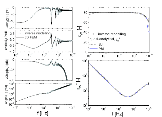
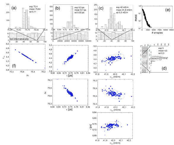
In Fig. 3 optimization results are represented in case of a coaxial transmission line filled with tap-water. The corresponding spectra obtained with the quasi-analytical approach as well as inverse modeling technique are represented in Figure 4. The optimization results are in close agreement with the expected parameters especially in case of the simple Debye-model. The appropriate bivariate scatter plots further indicate the expected correlation between and due to the limited accessible frequency range (see Figure 4).
3 RESULTS AND DISCUSSION
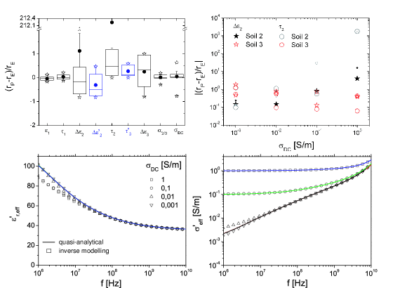
In Figure 5 the error statistics of the different relaxation parameters related to the expected parameters of Table 1 are represented for all investigated materials. The relative error of the relaxation time of process 3 is not included in the plot due to a high uncertainty related to the restricted frequency range. The error statistics clearly indicate an reasonable accuracy in the determination of the relaxation parameters of process 1 as well as the direct conductivity in agreement with experimental results [1, 24, 5]. This in addition shows the results of the obtained spectra in comparison with the quasi-analytical approaches. However, a serious limitation is observed in case of low values S/m leading to an increase in the uncertainty in the parameter estimation process (Figure 5, bottom). The uncertainty in the prediction of relaxation parameters and is strongly affected by the conductivity contribution (Figure 5, top/right). This suggests to separate conductivity effects prior to the analysis of the spectra especially in case of high conductivities S/m leading to a substantial decrease in the uncertainty. Moreover, the magnitude of the process in relationship to further overlying processes strongly affects the uncertainty of the parameter estimation process. In contrast, both relaxation time distribution parameters were estimated with reasonable accuracy.
4 CONCLUSION
The results show: (i) regardless of the underlying relaxation processes, the dielectric spectra can be determined in close agreement with the assumed input spectra and (ii) the relaxation behavior can be parameterized with reasonable accuracy if the relaxation frequency of the single processes is in the frequency range of the measurement. If is below or above the measurement range, than the accuracy of the estimated relaxation parameters strongly decreases. In context of spectra related to porous media it was found that the relaxation behavior of the free water contribution (primary -process) as well as the apparent conductivity contribution can be characterized in close agreement with experimental results. The low frequency process accounts for the low frequency dispersion as well as electrode polarization effects which is the most challenging process. The secondary process can be characterized, but the relaxation characteristics is strongly affected by the overlapping -process as well as the magnitude of the direct current conductivity contribution. To quantitatively relate the relaxation parameters to soil physico-chemical quantities (i) the measurement range have to be extended to lower frequencies, (ii) an informative prior have to be included in the optimization process, and (iii) the complexity of the relaxation model has to be constraint by means of a combination of relaxation models and mixture equations. In next steps, the results determined in parameterizing the the S-parameters will be compared with results obtained by classical parametrization of the dielectric spectra with quasi-analytical approaches based on the Geophysical Inversion and Modelling Library (GIMLi, see [25]).
References
- [1] N. Wagner, K. Emmerich, F. Bonitz, and K. Kupfer, “Experimental investigations on the frequency and temperature dependent dielectric material properties of soil,” IEEE Transactions on Geoscience and Remote Sensing, vol. 47, no. 7, pp. 2518–2530, 2011.
- [2] N. Wagner and A. Scheuermann, “On the relationship between matric potential and dielectric properties of organic free soils,” Canadian geotechnical journal, vol. 46, no. 10, pp. 1202–1215, 2009.
- [3] D. A. Robinson, C. S. Campbell, J. W. Hopmans, B. K. Hornbuckle, S. B. Jones, R. Knight, F. Ogden, J. Selker, and O. Wendroth, “Soil moisture measurement for ecological and hydrological watershed-scale observatories: A review,” Vadose Zone J., vol. 7, pp. 358–389, Feb. 2008.
- [4] K. Lauer, N. Wagner, and P. Felix-Henningsen, “A new technique for measuring broadband dielectric spectra of undisturbed soil samples,” European Journal of Soil Science, vol. 63, p. 224-238, 2012.
- [5] N. Wagner, M. Schwing, and A. Scheuermann, “Numerical 3-d fem and experimental analysis of the open-ended coaxial line technique for microwave dielectric spectroscopy on soil,” Geoscience and Remote Sensing, IEEE Transactions on, 2013, in print.
- [6] N. Wagner, B. Mueller, K. Kupfer, M. Schwing, and A. Scheuermann, “Broadband electromagnetic characterization of two-port rod based transmission lines for dielectric spectroscopy in soils,” in Proc. 1th European Conference on Moisture Measurement, Aquametry 2010 (K. Kupfer, ed.), (Weimar, Germany), pp. 228–237, MFPA Weimar, 2010.
- [7] A. Nicolson and G. Ross, “Measurement of the intrinsic properties of materials by time domain techniques,” IEEE Trans. Insturm. Meas, vol. IM-19, pp. 377–382, 1970.
- [8] J. Baker-Jarvis, M. D. Janezic, B. Riddle, R. T. Johnk, P. Kabos, C. L. Holloway, R. G. Geyer, and C. A. Grosvenor, “Measuring the permittivity and permeability of lossy materials: Solids, liquids, metals, building materials, and negative-index materials,” Tech. Rep. 1536, National Institute of Standards and Technology - NIST, 2004.
- [9] A. Gorriti and E. Slob, “Synthesis of all known analytical permittivity reconstruction techniques of nonmagnetic materials from reflection and transmission measurements,” IEEE Transactions on Geoscience and Remote Sensing, vol. 2, no. 4, pp. 433–436, 2005.
- [10] W. Weir, “Automatic measurement of complex dielectric donstant and permeability at microwave frequencies,” Proceedings of the IEEE, vol. 62, no. 1, pp. 33–36, 1974.
- [11] A. Gorriti and E. Slob, “Comparison of the different reconstruction techniques of permittivity from s-parameters,” IEEE Transactions on Geoscience and Remote Sensing, vol. 43, no. 9, pp. 2051–2057, 2005.
- [12] K. Zhang and D. Li, Electromagnetic theory for microwaves and optoelectronics. Springer, 2007.
- [13] N. Wagner, M. Schwing, A. Scheuermann, F. Bonitz, and K. Kupfer, “On the coupled hydraulic and dielectric material properties of soils: combined numerical and experimental investigations.,” in Proc. of the International Conference on Electromagnetic Wave Interaction with Water and Moist Substances (D. B. Funk, ed.), pp. 152–161, 2011.
- [14] D. A. Robinson, S. B. Jones, J. M. Wraith, D. Or, and S. P. Friedman, “A review of advances in dielectric and electrical conductivity measurement in soils using time domain reflectometry,” Vadose Zone J, vol. 2, no. 4, pp. 444–475, 2003.
- [15] P. Hoekstra and A. Delaney Journal of Geophysical Research, vol. 79, no. 11, pp. 1699–1708, 1974.
- [16] F. Hollender and S. Tillard, “Modeling ground-penetrating radar wave propagation and reflection with the jonscher parameterization,” Geophysics, vol. 63, no. 6, pp. 1933–1942, 1998.
- [17] T. Ishida, T. Makino, and C. Wang, “Dielectric-relaxation spectroscopy of kaolinite, montmorillonite, allophane, and imogolite under moist conditions,” Clays and Clay Minerals, vol. 48, no. 1, pp. 75–84, 2000.
- [18] T. J. Kelleners, D. A. Robinson, P. J. Shouse, J. E. Ayars, and T. H. Skaggs, “Frequency Dependence of the Complex Permittivity and Its Impact on Dielectric Sensor Calibration in Soils,” Soil Sci Soc Am J, vol. 69, no. 1, pp. 67–76, 2005.
- [19] N. Wagner, K. Kupfer, and E. Trinks, “A broadband dielectric spectroscopy study of the relaxation behaviour of subsoil.,” in Proc. of the International Conference on Electromagnetic Wave Interaction with Water and Moist Substances (S. Okamura, ed.), pp. 31–38, 2007.
- [20] N. Wagner, E. Trinks, and K. Kupfer, “Determination of the spatial -sensor characteristics in strong dispersive subsoil using frequency domain simulations in combination with microwave dielectric spectroscopy,” Measurement Science and Technology, vol. 18, no. 4, pp. 1137–1146, 2007.
- [21] R. Hilfer, “H-function representations for stretched exponential relaxation and non-Debye susceptibilities in glassy systems,” Physical Review E, vol. 65, p. 061510, 2002.
- [22] J. A. Vrugt, H. V. Gupta, W. Bouten, and S. Sorooshian, “A shuffled complex evolution metropolis algorithm for optimization and uncertainty assessment of hydrologic model parameters,” Water Resour. Res., vol. 39, pp. –, Aug. 2003.
- [23] J. Heimovaara, Timo, A. Huisman, Johan, A. Vrugt, Jasper, and W. Bouten, “Obtaining the Spatial Distribution of Water Content along a TDR Probe Using the SCEM-UA Bayesian Inverse Modeling Scheme,” Vadose Zone J, vol. 3, pp. 1128–1145, 2004.
- [24] N. Wagner and K. Lauer, “Simultaneous determination of the dielectric relaxation behavior and soilwater characteristic curve of undisturbed soil samples,” in Geoscience and Remote Sensing Symposium (IGARSS), 2012 IEEE International, pp. 3202–3205, IEEE, 2012.
- [25] M. Loewer, N. Wagner, and J. Igel, “Prediction of GPR performance in soils using broadband dielectric spectroscopy,” in Proc. of the International Conference on Electromagnetic Wave Interaction with Water and Moist Substances, ISEMA (K. Kupfer, ed.), p. this issue, 2013.