Congestion-Aware Path Re-routing Strategy for Dense Urban Airspace
Abstract
Existing UAS Traffic Management (UTM) frameworks designate preplanned flight paths to uncrewed aircraft systems (UAS), enabling the UAS to deliver payloads. However, with increasing delivery demand between the source-destination pairs in the urban airspace, UAS will likely experience considerable congestion on the nominal paths. We propose a rule-based congestion mitigation strategy that improves UAS safety and airspace utilization in congested traffic streams. The strategy relies on nominal path information from the UTM and positional information of other UAS in the vicinity. Following the strategy, UAS opts for alternative local paths in the unoccupied airspace surrounding the nominal path and avoids congested regions. The strategy results in UAS traffic exploring and spreading to alternative adjacent routes on encountering congestion. The paper presents queuing models to estimate the expected traffic spread for varying stochastic delivery demand at the source, thus helping to reserve the airspace around the nominal path beforehand to accommodate any foreseen congestion. Simulations are presented to validate the queuing results in the presence of static obstacles and intersecting UAS streams.
Index Terms:
Uncrewed aircraft system (UAS), UAS Traffic Management (UTM), congestion-aware path planning, Discrete-time queuing theoryI Introduction
With the rapid growth in the number of uncrewed aircraft systems (UAS) being deployed for on-demand delivery applications, severe congestion is foreseen in the urban airspace. There is a need for structuring the airspace to mitigate this congestion. Delivery applications is urban airspaces would normally require UAS to travel on preplanned paths between source-destination pairs. Geofencing these paths can physically separate a UAS trajectory from other UAS, as well as static obstacles. However, intersecting UAS trajectories are inevitable, especially in dense traffic scenarios. Increased traffic on these paths due to increasing delivery demand results in severe conflicts among the UAS. Further, the increasing number of conflicts in confined geofenced air volumes could be detrimental to UAS safety. Such limitations are majorly due to treating UAS traffic as a road-like network or air traffic, where UAS are restricted to the preplanned paths and air volumes. To overcome this problem, we propose in this paper an airspace design and a congestion mitigation strategy that utilizes the airspace surrounding the preplanned path and dynamically generates local paths for UAS. These paths are opted for when the preplanned paths are congested. We also suggest an approach for estimating the expected air volume that would be utilized as a function of the probabilistic occurrence of congestion. Such airspace can be adaptively reserved beforehand to accommodate any foreseen congestion.
Background and Literature: Several government and private agencies [1, 2, 3] have developed different airspace designs to enable beyond-visual range UAS operations. These designs impose structural constraints on UAS’s degree of freedom (DoF) to maximize airspace safety and capacity at the expense of introducing time delays in UAS flights. Broadly, the structures proposed suggest segmenting the airspace and restricting the UAS in an air matrix (discrete UAS DoF) [4]; in a network of virtual air geofenced corridors (unidirectional UAS traffic flow in an enclosed air corridor volume) [5]; or in geo-vectored altitude layers, where UAS heading vector range is limited in each altitude layer and the altitude layers are interconnected by vertical ascend or descend corridors) [6]. UAS safety risk is a probabilistic belief on collision occurrence among UAS. In [7], the event where the separation between UAS is below a threshold is termed an intrusion. An anticipated intrusion in a prescribed look-ahead time window is termed a conflict. Whereas congestion is an accumulation of UAS in a predefined region that eventually leads to increased conflict risk. The airspace designs have an intrinsic ability to reduce the occurrence of collision due to the constraints that it imposes on the UAS traffic.
In air matrix design, the airspace is tessellated into a cellular grid, and online path-planning strategies such as Rapidly exploring Random Trees (RRT), skeleton maps [8, 9] were proposed that generate optimal and risk-aware trajectories for UAS. However, with the increasing number of UAS, these strategies lead to an unstructured and unpredictable traffic pattern.
In altitude-layered airspace, the intrinsic safety can be improved if the UAS is capable of sensing and avoiding (SAA) the intrusions [10] or can mitigate conflict risk by preflight or in-flight conflict detection and resolution (CDR) [11, 12].
Though the SAA and CDR are adequate at individual UAS levels, these approaches perform poorly in congested traffic scenarios. In the study conducted by [13], beyond a critical demand, the SAA can no longer execute avoidance maneuvers without colliding with neighboring UAS. Whereas the in-flight CDR suffers from domino effects and spillback conflicts, which can severely destabilize the UAS traffic [14, 15]. A solution to this problem as proposed in this paper, is to mitigate congestion and prevent high UAS density regions from forming than to allow UAS to proceed and encounter conflicts in dense regions.
The analytical study in [16] suggests segregating UAS into altitude layers as prima facie for mitigating congestion.
In [14], when two or more UAS conflict, these UAS are collectively enclosed in a virtual disk and labeled as congested. Any UAS in its vicinity locally re-route, avoiding this disk until the conflicts in the disk are resolved. In [17], the airspace is tesselated into cells, and the cell is said to be congested if the number of pre-planned paths occupying the same cell is greater than the cell capacity. Similarly, in [18], a region is congested if the expectation of UAS encountering conflict with two or more UAS is above some threshold.
The papers [19, 20, 21] present strategies for mitigating congestion in the air corridor networks. In [19], the UAS traffic is modeled as fluid queues, and the congestion is mitigated by controlling the UAS inflow and outflow rate for each corridor in the network. In [20],
the velocity of the trailing UAS is reduced proportional to the weighted sum of UAS inter-separation distances in the congested volume. In [21],
the congestion is mitigated by solving a traffic assignment problem such that the number of UAS routed on each corridor results in an equitable UAS density distribution in all corridors. In [18, 17, 21], the mitigation strategy is spatial and does not capture congestion in the temporal sense, forcing new incoming UAS to take long detours. Whereas in [19, 20], intermittent local congestion events affect the throughput of the entire corridor network. This limitation is because the UAS is always restricted within air corridors despite airspace being available in the surrounding airspace.
Our Contributions: In this paper, we present a distributed congestion mitigation strategy where UAS decisively opts for local alternative paths upon encountering congestion in its preplanned flight path and reverts when congestion reduces. Such path re-routing response of UAS ensures no further UAS inflow into congested regions and upper bounds the number of conflicts in the region. The proposed strategy can handle congestion contingencies due to system failure, rogue agents, intersecting UAS streams, and time-varying stochastic delivery demand. The main contributions of this paper are as follows.
-
1.
A novel distributed congestion mitigation strategy is proposed, imposing congestion-aware and preference-based heading structural constraints on UAS degree of motion.
-
2.
Demonstrating how the proposed strategy adapts to the increasing UAS demand and dynamically creates parallel air corridors, thus offering intrinsic safety for high UAS traffic demand.
-
3.
Development of queuing-based models for estimating the expected spread of the UAS traffic stream when every UAS implements the proposed congestion mitigation strategy.
The paper is organized as follows. The workspace for the congestion mitigation problem is defined in Section II. Section III introduces congestion, the heading structural constraints being imposed, and the proposed congestion mitigation strategy employed by UAS. Section IV presents queuing models to study the emerging traffic behavior as a function of the UAS traffic demand and structural constraints. Section V presents simulations that demonstrate the increased intrinsic safety and resemblance of UAS traffic to the parallel air corridor network. Section VI concludes the paper, emphasizing the advantages of the proposed mitigation strategy.
II Problem Definition
This paper presents traffic analysis for a UAS traffic management (UTM) framework driven by stochastic delivery demand. The UTM environment has static obstacles and several source-destination pairs. The delivery service provider deploys a UAS for every customer requesting delivery on a specific source-destination route, and such requests recur stochastically. Accordingly, at the source location, a time-varying geometrically distributed request for UAS is assumed with bounded request rate , where is the maximum request rate. The time axis is divided into slots of time units and indexed with . We assume that though multiple requests are received in a given time slot, only one request among them is randomly chosen, for which a UAS is deployed at the start of the next timeslot. The remaining requests are dropped. The probability that a UAS would be deployed in a timeslot is given by .
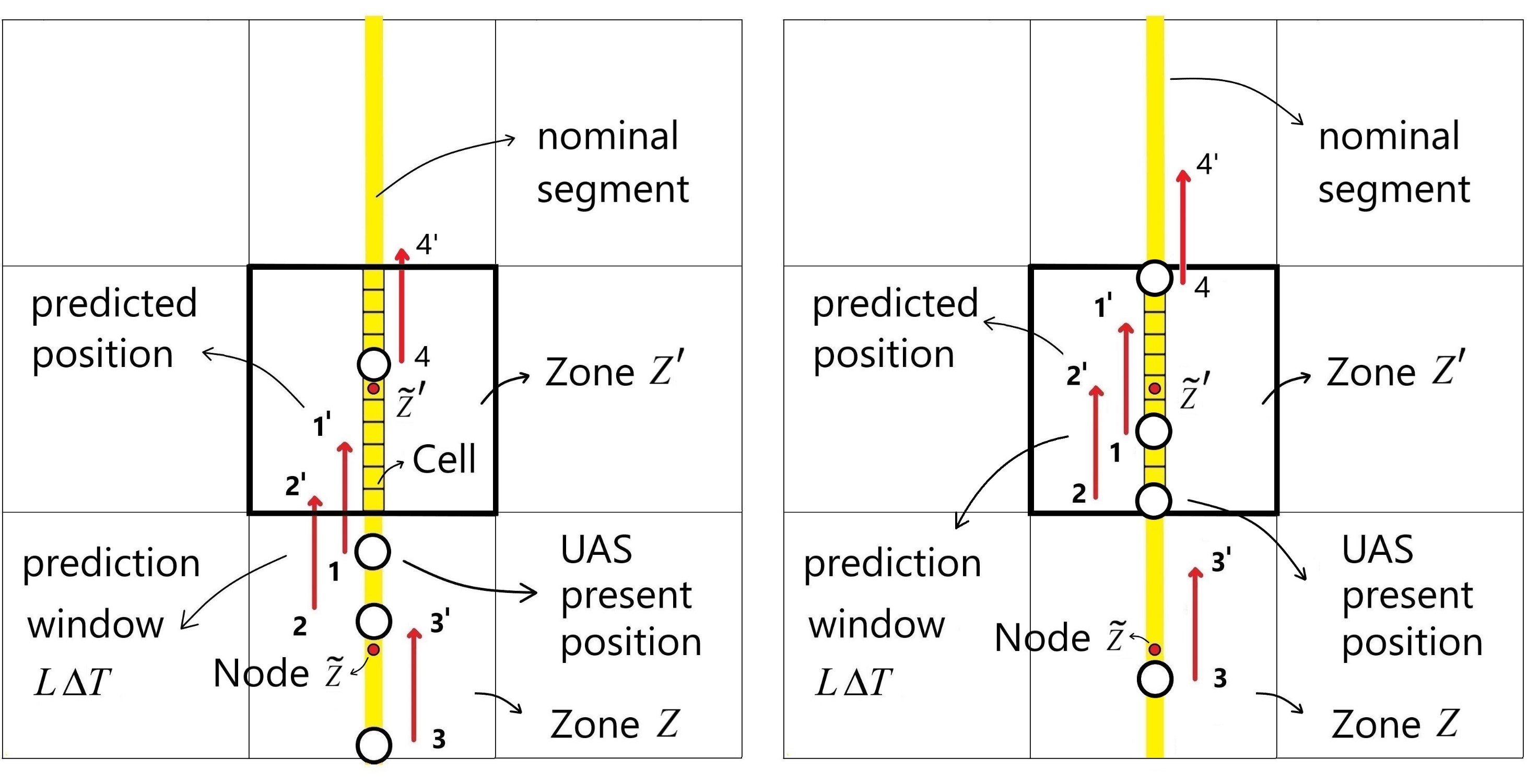
The workspace is assumed to be a bounded horizontal stretch of air volume containing the given source-destination pair. It is tessellated into a connected grid of a finite number of identical cells. As the static obstacles are of varying heights, some may intersect the cells of this workspace. We define a geometric center called the cell center for each static obstacle-free cell (refer Fig. 1). The motion of a UAS leaving a cell center and traveling in a straight line to reach a neighboring cell center is referred to as a transition. The traversal of UAS in the workspace is modeled as successive transitions from one cell center to any of its neighboring cell centers. We assume that the UAS takes seconds to transition between neighboring cell centers. Two UAS that are cells spatial separated are equivalently slots () temporal separated.
The UTM is assumed to prescribe a nominal path connecting cell centers between any source-destination pair. We assume this path would be approximated by connected straight-line segments passing through cell centers. Since the UAS requests are assumed geometrically distributed with request rate , the inter-separation distance between UAS transitioning on the nominal path (in time slots) is also geometrically distributed and is given by the distribution as follows.
| (1) |
where is the probability that the inter-separation distance between UAS is time slots. If between any two UAS, these two UAS are present in a cell and counted as an intrusion. Analogously, , the probability of an intrusion in the look-ahead time window is the conflict risk ().
Let time slots be the threshold on UAS inter-separation distance for defining congestion. Consider an arbitrary region in which more than UAS are present, with the inter-separation distances between them being less than . We assume positive correlation of with and negative correlation with , that is, . The relation means there is an increased risk of conflict when there are UAS that are time slots closer to each other. Avoiding such higher-risk regions is preferable. These regions are referred to as congested regions. Here, is a UTM design parameter.
The requests are recurring, hence there is a stream of UAS traffic flowing in the nominal path from source to destination. The traffic in the path, right ahead in front of a UAS, is its upstream traffic. The traffic trailing behind the UAS is its downstream traffic. When is large, is high; thus, the chances of a UAS encountering congestion on its upstream is high. When the probability of congestion increases, there is a requirement to generate alternative parallel paths (dependent on the request rate) that avoid congested regions.
The nominal path is a reference path given to the UAS. However, the UAS is free to opt for any of those cell centers in its neighborhood that do not violate the constraints set by the UTM. The main objective of this paper is to propose a distributed congestion mitigation strategy for the UAS. Using this strategy, individual UAS can dynamically generate local parallel paths for itself in the unoccupied airspace in a structured manner, following which the UAS bypasses congested regions in its local neighborhood. When the request rate is low, the UAS traverses along the nominal flight path. However, in the event of congestion on the nominal path, a certain number of UAS present in the downstream are diverted onto the parallel paths. As the request rate increases, the frequency of the congestion event increases. The number of UAS that would be diverted on parallel paths also increases, causing congestion on the parallel paths as well. Then, UAS downstream would have to opt for parallel paths further outward from the nominal path. When congestion reduces, the UAS on parallel paths tends to close in on the nominal path. In this process of mitigating congestion, there would be a change in the area occupied by the UAS stream around the nominal path with variation in the request rate.
The above idea is illustrated in Fig. 2. The UAS only relies on the nominal path information from UTM and the positional information of UAS present in its vicinity to determine congested regions and generate local parallel paths. For the UAS traffic streams routed between source-destination pairs, we intend to demonstrate and analyze the extent of the UAS traffic spread around the nominal path as a function of the request rate. The paper also extends congestion mitigation to scenarios where the inter-separation distances between UAS of intersecting UAS traffic streams fall below the threshold .
III Congestion Mitigation Methodology
The nominal path between the source-destination pair is segmented into a connected chain of straight-line segments. The set of cells through which the straight-line segment passes is called a nominal segment, with a start and an end cell defined for each segment. The proposed strategy deals with congestion in each nominal segment separately. A unit vector directed from start to end is called an upstream vector, and that directed from end to start is called a downstream vector. To identify a region as congested, we first need to geometrically define the region, for which, we partition the workspace as follows.
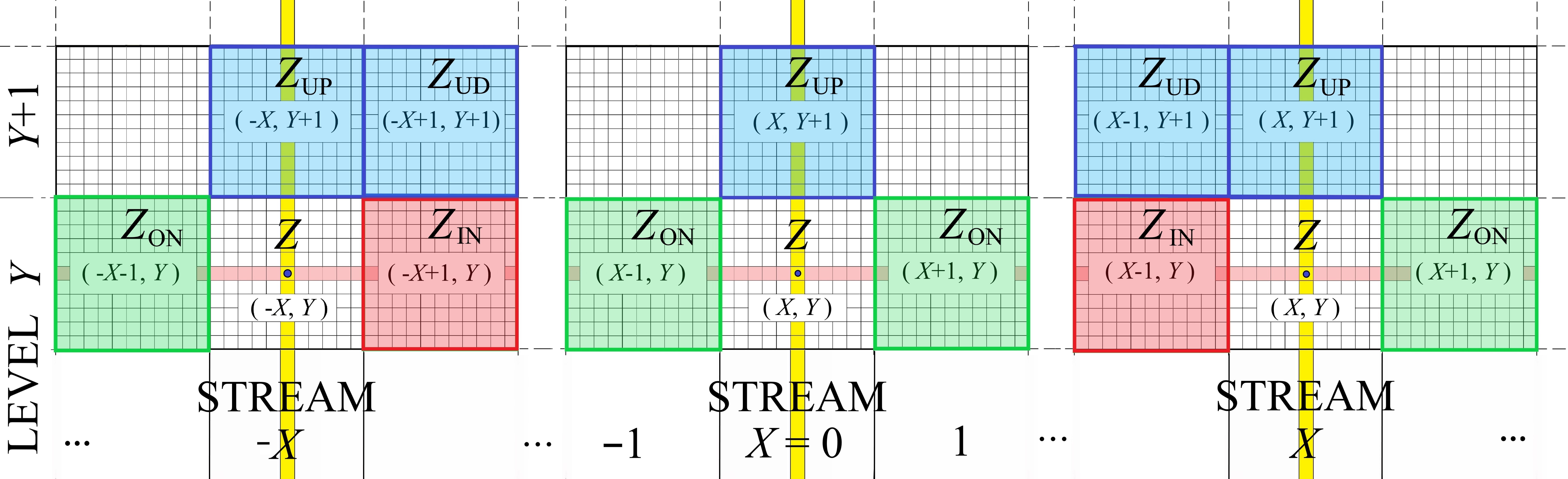
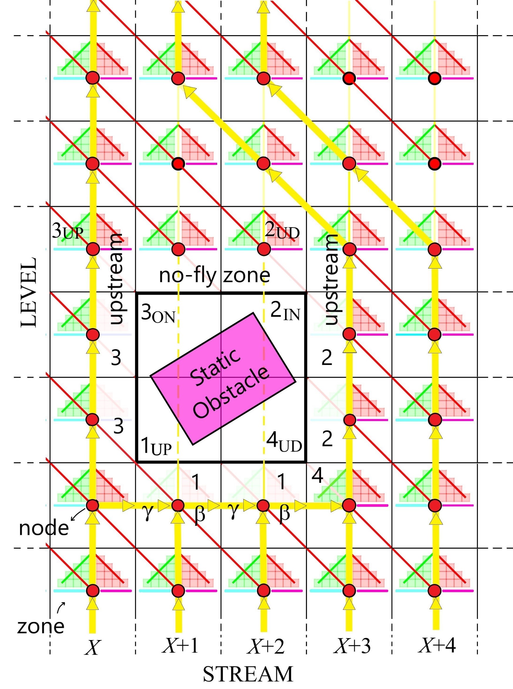
Assume the UAS are identical in all aspects and have a slot look-ahead time window to predict where other UAS would be in the next time ahead. The cells in the nominal segment (start and end included) that are time slots apart are called nodes (shown in Fig. 3(a)). With each node as a geometric center, the set of cells enclosed in a square region with edge length timeslots (an edge parallel to the segment) is called a nominal zone. The eight square regions (of timeslots edge length) surrounding the nominal zone are called zones and form the neighborhood of the nominal zone. Similarly, we may define the neighborhood for any arbitrary zone. We assume a finite grid of identical zones for each nominal segment to facilitate alternative path generation in the event of congestion. The grid is so positioned that the nominal zones are a subset of the grid and bisect the grid (shown in Fig. 3(b)). The length of the grid (that is the length of the nominal segment) is significantly larger than the width. The start cell, end cell, and width of the grid for two connected nominal segments are chosen such that the respective grids do not intersect. A stream-level tuple notation is used for referring to zones in the finite grid, where Stream and Level and, and are positive integers (refer Fig. 3(b)). The nominal zones are called Stream zones denoted with tuple , where denotes the zone level in the upstream direction. , denote the nominal zones containing start and end cells, respectively. We define the congested regions as follows.
Definition 1.
A zone is said to be congested if or more than number of UAS are present in the zone.
and are UTM design parameters. Note that the congestion in the zone is due to UAS transitioning on the given source-destination route as well as due to any exogenous UAS coexisting in the workspace. The grid construction is UAS-agnostic. The UAS can extract the grid geometry from the nominal segment information shared by the UTM. Within the zone, the heading of the UAS would be restricted so that UAS would only transition on a subset of cells. The heading constraint is position-dependent, for example, when UAS is in the nominal segment it is restricted to transition in the upstream direction. A UAS in a zone can detect or communicate with other UAS coexisting in the zone and its respective neighborhood. By knowing the UAS present positions, the heading constraint imposed, and that any UAS would complete one transition in one timeslot, we assume the UAS using a linear kinematic model can predict other UAS state information (position and heading) time ahead with sufficient accuracy.
The UAS on reaching a node needs transitions on the nominal segment to reach the neighboring zone. Since a slot look-ahead time window is assumed, when the UAS is at a node and finds the neighboring zone is likely to turn congested in the next slots, then the UAS could decide to avoid the neighboring zone.
Definition 2.
From the perspective of a UAS in zone (depicted in Fig. 4), the neighboring zone will likely be congested if the number of slot look-ahead UAS predicted positions in zone is greater than or equal to .
The congestion definition introduced for the nominal zone applies to all the zones in the grid. However, the decisions of UAS present in an arbitrary zone are only influenced by congestion occurrences in one or two of its neighboring upstream zones, which are,
-
1.
if
-
2.
if
-
3.
if
For ease of notation, we refer to the neighboring zones of interest as shown in Fig. 5. is an upstream neighbor, is an inner neighbor (zone closer to the Stream zone than zone ), is an upstream inner diagonal neighbor and, is an outer neighbor (zone farther from Stream than zone ). Note that and are defined only when . The zone notation can be extended to respective nodes as well. By interconnecting the nodes with respective nodes, , we have parallel segments referred to as Stream segments.
At node , if the UAS decides to avoid the zone , it generates a piece-wise re-route path (a sequence of the number of transitions to take in a specific heading direction). The UTM provides a heading-reference directed graph to the UAS present in an arbitrary grid level as shown in Fig. 6. For a zone , the graph comprises of
-
1.
an path of cells in the upstream direction (hereafter referred as heading) connecting node with ,
-
2.
a path of cells in the inward diagonal direction ( heading) connecting node with ,
-
3.
a and a path of cells each in the outward lateral direction ( heading), connecting zone with node and node with zone , respectively. These are alternate paths for UAS in , in case the turns congested. The paths including node are collectively referred to as path.
-
4.
number of inward diagonal ( heading) and number of outward diagonal ( heading) parallel paths, connecting and path with path, respectively. These are alternate paths for UAS in the cells of and path, in case the turns uncongested.
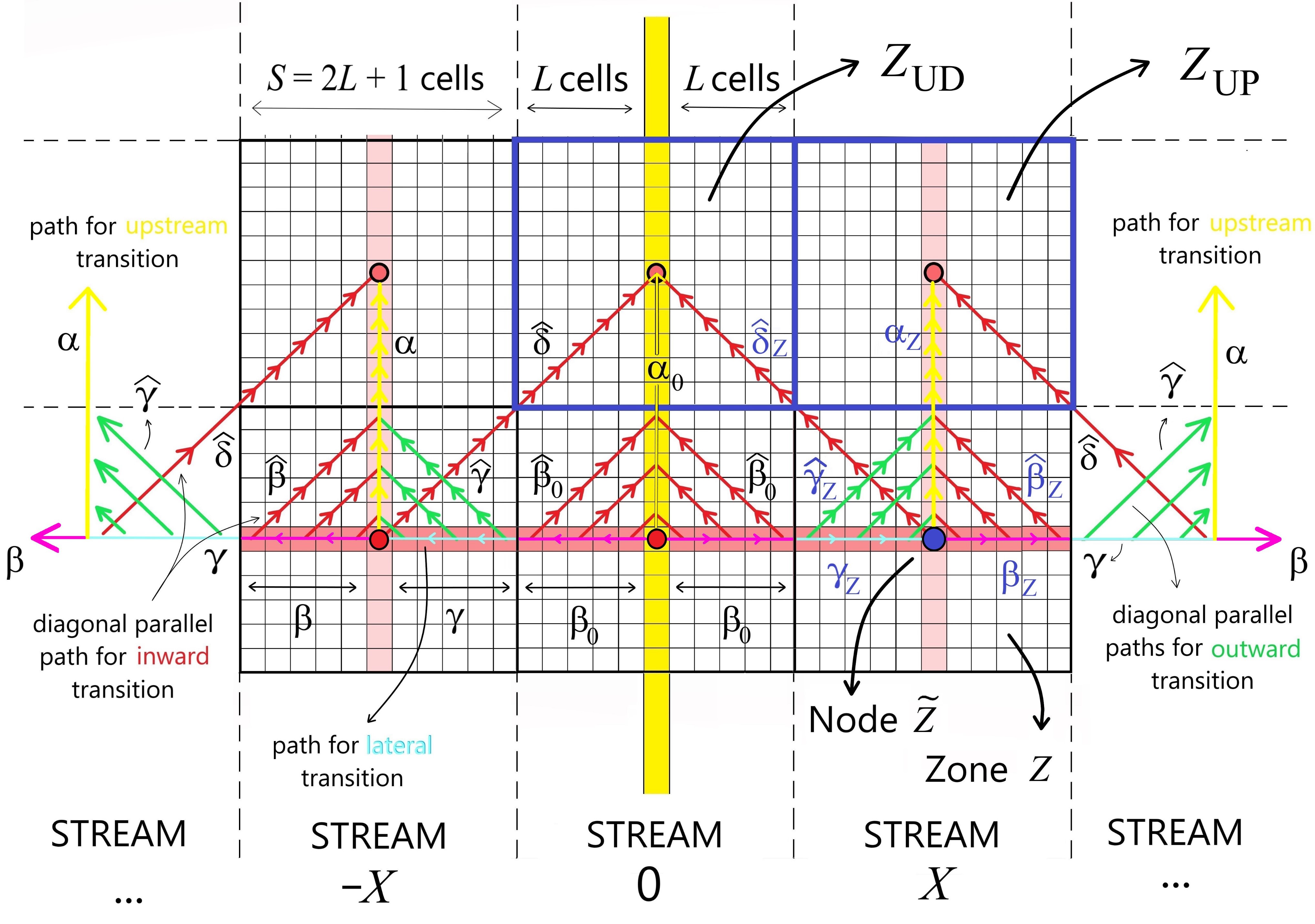
As a special case, the graph for Stream zones comprises an upstream path, two paths with opposite headings directed laterally outward from node, and number of inward diagonal paths. For notation convenience, we use , with subscript referring to the paths in the zones respectively. We ignore the subscript when referring to an arbitrary zone.
The rule-based congestion mitigation strategy for the UAS foreseeing congestion in its and zones is as follows. The following rules assume the UAS is transitioning on a Stream segment, . The heading reference graph is symmetric about the Stream segment; hence similar rules when do hold.
Rule 1.
The UAS present in zone identify respective and zones as congested or uncongested following Definition 2.
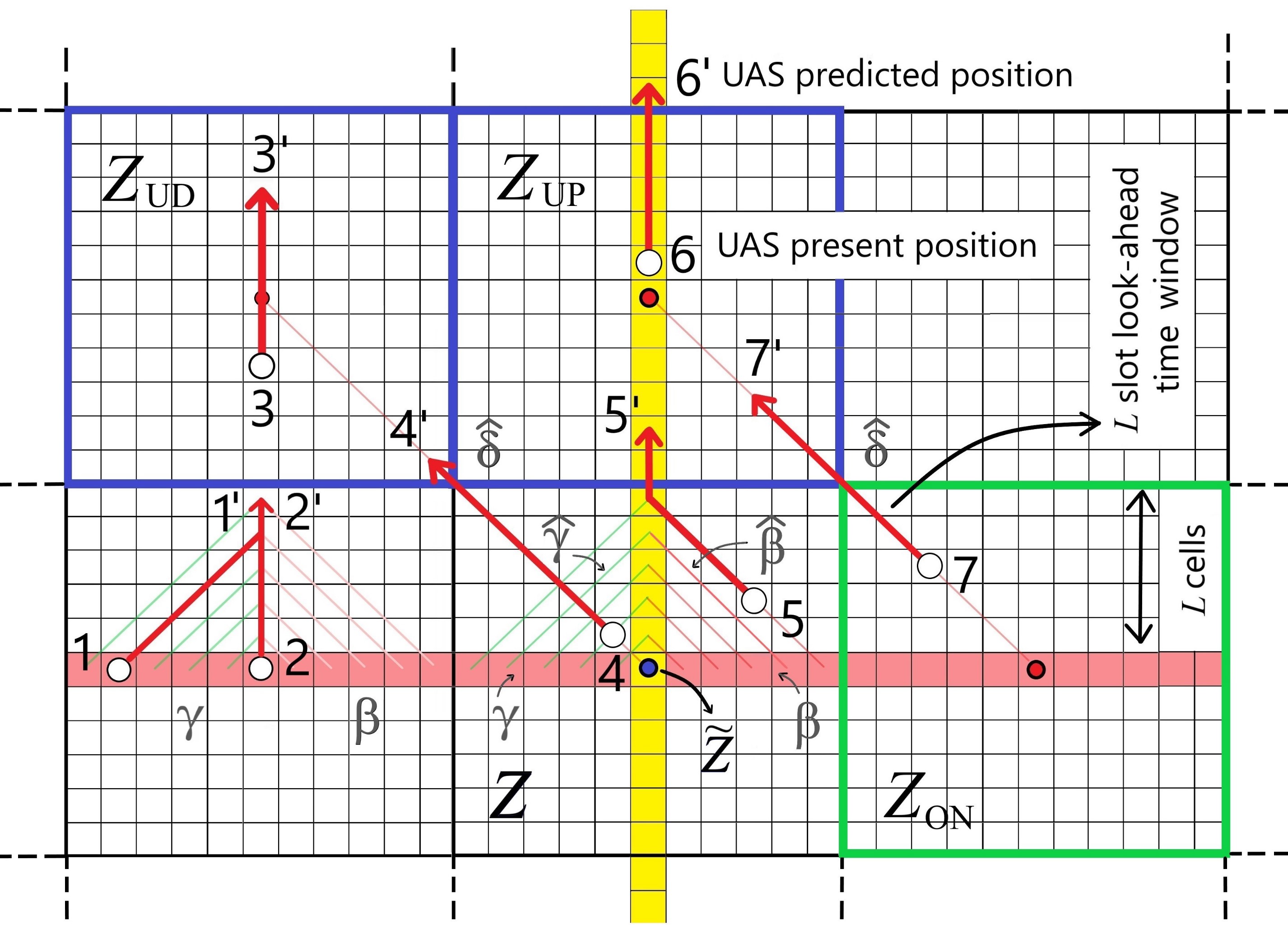
Note that the UAS is restricted to transition on the heading-constrained graph shown in Fig. 6. Under the above structural constraint, among the UAS present in the zone , the slot look-ahead predicted positions of only those UAS transitioning on paths lie in zone and are responsible for congestion. Similarly, predicted positions of UAS transitioning on path lie in zone (refer Fig. 7).
Rule 2.
In a given time slot, if the UAS present in path finds zone congested, then the UAS executes one lateral transition in the heading direction.
In Fig. 8, if is congested in timeslot , then in timeslot UAS in positions would be in positions respectively. A zone congested at one timeslot may or may not be congested in the next. Only myopic position predictions ( slot look-ahead) are possible for UAS transitioning on , as it is uncertain whether these UAS would continue transitioning in direction or not. Hence, these UAS are excluded in the Definition 2. If the UAS that has entered the path (UAS in position in Fig. 8) finds the zone congested for successive slots, the UAS ends in the path. Similarly, if a UAS that has entered the path (UAS in position in Fig. 8) finds the zone congested for successive slots, it reaches node .
The duration for which zone remains congested and the number of UAS present in the zone when congested depends on the exogenous UAS in as well. For the UAS laterally transitioning on path, with each successive outward transition, the UAS belief that the respective would always remain congested is reinforced. Hence, the UAS that has transitioned longer on the path rather prefers to avoid and progress to , believing that when the UAS enters path the upstream neighbor of would be uncongested. The UAS that has just entered node from the downstream zones passively prefers to move towards if uncongested. Whereas, the UAS presently in path had previously avoided the zone believing that when it entered path the would have been uncongested. The UAS in the path actively prefers to move towards zone , thus has a higher preference than the UAS in the node and path. Each UAS present in path is marked with a value reflecting the above time varying UAS preference to move towards zone. The UAS preference is modeled as a linear function of the UAS relative position on the path, given by
| (2) |
UAS having zero would mean the UAS is currently at node . UAS with negative prefer reverting (inward diagonal transition) to the zone. The UAS having positive prefer progressing (outward diagonal transition) to the zone if the zone turns uncongested. Preference is information shared among UAS transitioning in path or can be computed using positional information , enabling the UAS to distributedly decide which UAS should proceed upstream when the respective zone turns uncongested.
Rule 3.
If in a given time slot the zone turns uncongested, then among the UAS laterally transitioning on path, that UAS which has the highest preference would proceed towards the zone. The remaining UAS execute one lateral outward transition on respective paths.
Applying Rule 3 in Fig. 8, if UAS are present in position , then UAS in position proceeds to position ‘a’, whereas UAS in position transition to position respectively. The UAS in position proceed to position ‘b’ if and only if no UAS are present in positions and respectively. Corresponding to each value of , we have a piece-wise or or path that connects the path with node . Thus, a total of paths exists. Further, the UAS in path needs transitions on respective path to reach the node (refer Fig. 9).
Rule 4.
Following Rule 3, the UAS in the path that has the highest preference opts the following path to relatively transition upstream and reach node.
-
1.
If , then UAS is at node and proceeds with successive transitions in heading direction.
-
2.
When then UAS proceed with successive diagonal transitions in heading direction followed by upstream transitions in heading direction.
-
3.
When then UAS proceed with successive diagonal transitions in heading direction followed by upstream transitions in heading direction.
The following rules are for handling contingencies and exceptional scenarios. The UAS heading in and ( or ) direction may simultaneously reach the node in some time slot and encounter conflict. If conflict is not resolved, then following rules 2-4, the UAS will thereafter always conflict with each other for cell occupancy.
Rule 5.
In a given time slot, if a UAS in path is in conflict at node with a UAS from downstream, then the UAS in path is assigned preference . Irrespective of zone being congested, the UAS with executes a conflict resolution maneuver (shown in Fig. 10(a)) and then proceeds with upstream transitions in heading direction to reach .
The Conflict Detection and Resolution (CDR) methods suggested in [22, 23, 24] can be applied for conflict resolution maneuvers. The UAS is assumed to be enclosed in a virtual cylindrical disk of a predefined safety radius. The cells are large enough that during the spatiotemporal resolution maneuver, the safety disks do not overlap. However, the emphasis is on the UAS at cell center encountering conflict in time instant should reach neighboring cell center by time instant . The UAS is free to accelerate or decelerate about the nominal velocity to achieve the above time synchronization. During the conflict, the UAS executing conflict resolution maneuver (the UAS with ) has the highest preference. Hence, irrespective of zone being uncongested, the remaining UAS in path proceeds with one outward lateral transition.
Rule 6.
(Descend condition) In a given timeslot, if the downstream UAS enters node and finds the zone uncongested with no UAS present in path, then (irrespective of being uncongested or conflict at node ) the downstream UAS proceeds with successive transitions in the heading direction (shown in Fig. 10(b)) and reaches the node.
The UAS heading in and direction would never reach the node simultaneously because of the descend condition and hence, no conflict. However, the UAS transitioning in and directions may encounter conflict in some time instant. The conflict can be resolved by momentarily accelerating and decelerating the UAS. However, once the conflict is resolved, the UAS should reach their next destined cell centers in the time instant. While UAS is transitioning on the heading-constrained graph, the UAS may encounter zones that are occupied by static obstacles. The smallest rectangular zone cluster that encloses the static obstacle is demarcated as a no-fly zone.
Rule 7.
(Presence of static obstacle) For a UAS in zone , if the zone is a no-fly zone, then the UAS perceives as always congested. If the or zone is a no-fly zone, then the UAS perceives to be always congested. If the zone is a no-fly zone, then the UAS perceives the zone as always uncongested (refer Fig. 11).
As the UAS in the zone marked in Fig. 11 always perceive zone congested, by Rule 2, these UAS would certainly transition along path every successive timeslot. Hence, the -slot look ahead positions of these UAS can be determined and are included in the Definition 2.
Rule 8.
In a given timeslot, if the UAS is at Stream node and finds the zone congested, then it randomly opts either of the two heading directions with probability and and executes one lateral outward transition in the chosen heading direction.
Rule 9.
In a given timeslot, if the UAS present in node find the zone uncongested. Following Rule 6, either of the UAS in node or descends to with probability and respectively.
is a UTM design parameter to introduce bias in the traffic distribution about the Stream segment. It is useful when static obstacles or congestion hot spots due to exogenous UAS in the workspace are known apriori.
When every UAS in the finite grid follows the proposed rule-based congestion mitigation strategy, the emerging UAS traffic behavior resembles a parallel air corridor network, with no more than UAS in any zone and the number of active corridor streams (that is, the UAS traffic spread) adapting to the UAS demand (). When a new source-destination route is being planned for a given , the nominal path for the route, the finite grid, the parameters (zone dimension), (minimum number of UAS in the zone for congestion), and are chosen such that the expected traffic spread on this route does not interfere with existing hot spots. The expected UAS traffic spread could be estimated using queuing theoretical models presented in section IV. If is small, more UAS will transition outward; thus, more traffic spread. can be increased to lower the spread, compromising intrinsic safety. If is lower, denser traffic will flow on the left of Stream segment, hence more spread on the left and vice versa. However, if any nominal segment on the route need must pass through the hot spot intersecting the exogenous UAS traffic streams, we assume,
Assumption 1.
The nominal segment can be intersected by at most one exogenous traffic stream and must intersect orthogonally. The start cell, the end cell, and the finite grid for the nominal segment must be chosen such that the exogenous stream does not pass through any path in the grid.
The exogenous stream could be in the workspace or out of the plane as depicted by the air corridor in Fig. 3(b).
Assumption 2.
The inter-separation distances between UAS in the exogenous streams are geometrically distributed.
Assumption 3.
The traffic flow on the new source-destination route is affected by UAS in the exogenous traffic stream. However, the exogenous stream remains unaffected by the new incoming traffic flow.
The proposed mitigation strategy works even if the above assumptions are violated, as long as the slot look-ahead positions of UAS in the exogenous streams can be predicted or communicated (refer Fig. 12). Assumptions 1-3 have been stated to develop tractable queuing models for estimating expected traffic spread. Queuing analysis for the more general case is beyond the scope of this paper.
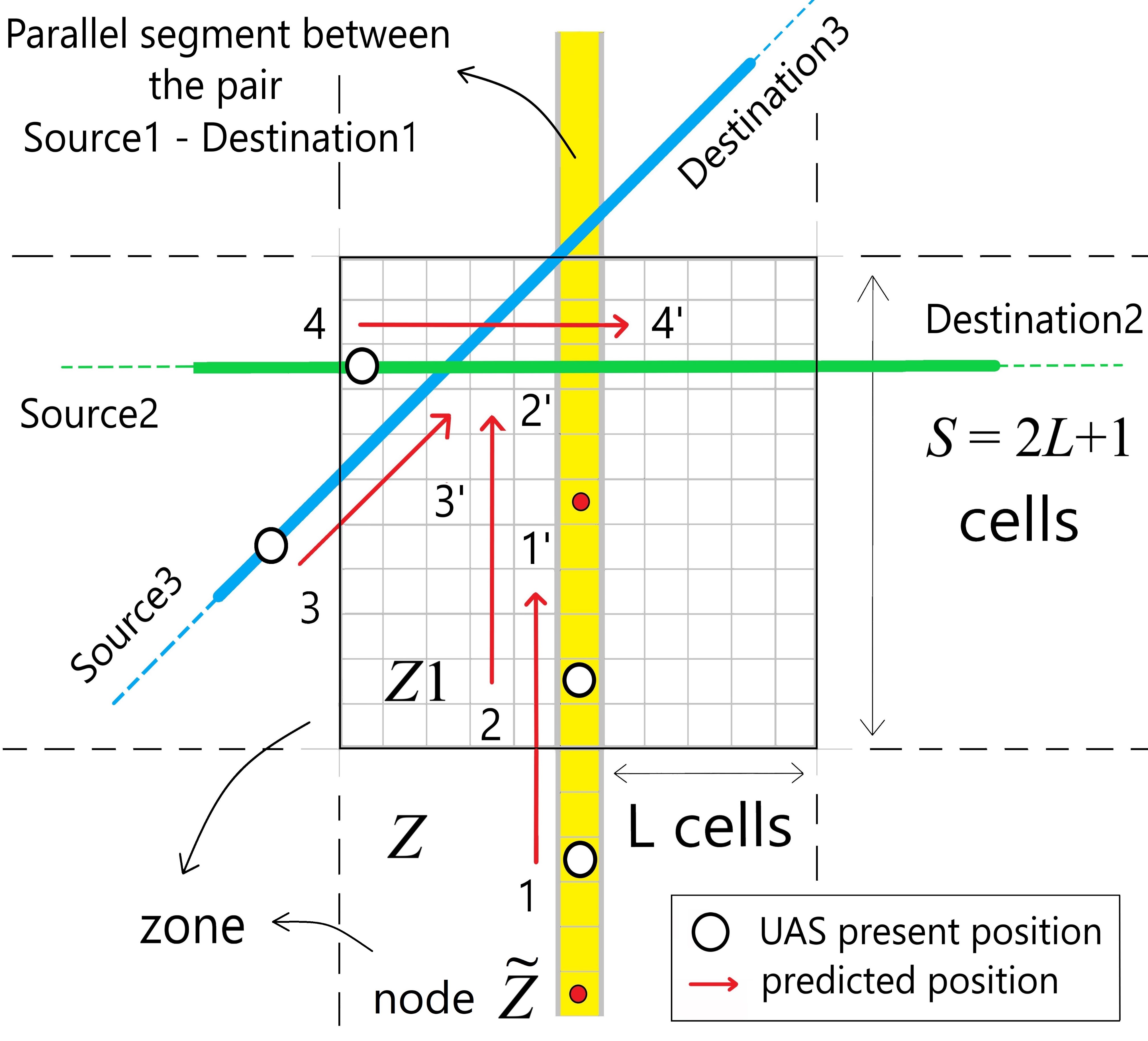
The UAS transitioning on the new route does encounter conflicts with UAS in the exogenous streams. However, for these UAS, the proposed congestion mitigation strategy guarantees no more than conflicts in any zone in the worst case. Here again, the conflicts are resolved by momentarily accelerating and decelerating the UAS, and once the conflict is resolved, the UAS must reach the destined cell center in the same time slot. If the exogenous stream is out of the plane, then in any timeslot at most one exogenous UAS exists in the zone. However, if the exogenous stream is in the workspace, the stream perpendicularly intersects the zone (Source2-Destination2 shown in Fig. 12), thus at most exogenous UAS can exist in any timeslot. If is the probability that an exogenous UAS enters a zone in a given timeslot, then the number of exogenous UAS in the zone is binomially distributed, with the expected number of exogenous UAS in the zone given by,
| (3) |
As a consequence of assumption 3, for the zones on the new route intersecting the exogenous stream must be greater than . Only then will the UAS transitioning on the new route cross the exogenous stream.
IV Congestion queuing model
We adopt the discrete-time queuing theory [25, 26, 27, 28] for estimating the expected number of UAS present in any zone , , . We define the queuing system , its servers, and queues as follows. Further, we will introduce sufficient supplementary variables so that the resulting queuing system state would be a Markov chain. As discussed in Fig. 7, for UAS transitioning in and paths, respective slot look-ahead positions are in zone and are responsible for congestion. We associate the zone with a queuing system , that comprises of cells belonging to and and paths. Following the rule-based congestion mitigation strategy, the UAS that enter this system of cells () are arrivals in queuing theory terminology. The downstream UAS that enter the system via node are referred to as nodal arrivals. Along with nodal arrivals, UAS in zones and enter the system via a cell that is not node. These UAS are referred to as non-nodal arrivals. The nodal and non-arrivals are denoted with random variables , and , respectively in Fig. 13. Note that if there is an arrival in time slot , and otherwise. Note that both and are bernoulli distributed and by Rule 6 (descend condition), in a given time slot both will not be 1 simultaneously. Thus, we merge the nodal arrivals as .
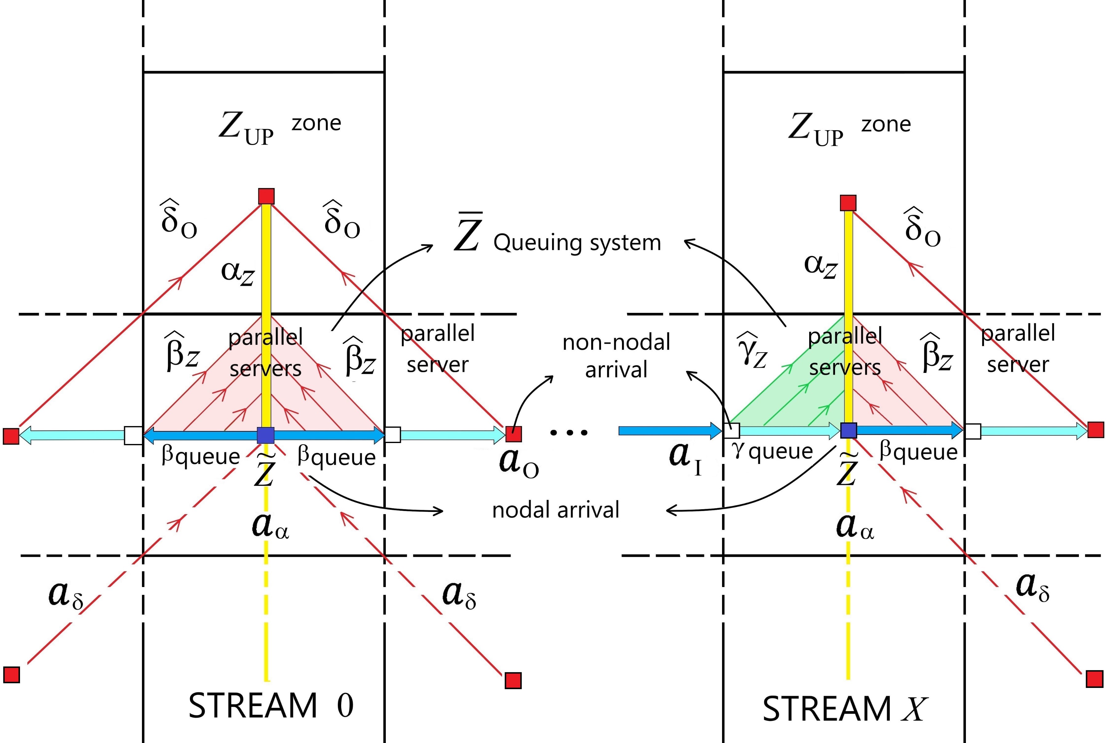
The paths summarized in Fig. 9 along with the path are the parallel servers of the system. The UAS transitioning on these paths are said to be in service. The UAS that has completed transitions on any of the paths is said to have received slots of service, and on reaching the node is said to have departed the queuing system. A UAS entering service needs transitions on any of the paths to reach node. Thus, irrespective of the parallel server and the time slot in which the UAS enters service, the service time is slots (that is time units). Let are random variables such that, at time slot , indicates that there exists a UAS that has received slots of service and otherwise. implies that a UAS has entered service in the previous time slot, and implies that a UAS would depart the system in the next time slot. A UAS that has received slots of service by time slot would have received slots of service by time slot. Hence,
| (4) |
where is the probability generating function (PGF) of limiting probability distribution of the random variable defined as,
| (5) |
The UAS in the exogenous stream passing through zone also contribute to congestion in . Corresponding cells through which the stream passes are appended in system . By Assumption 2, the inter-separation distances between UAS present positions, as well as between the slot look-ahead predicted positions, are geometrically distributed. Statistically, there is no difference between the counting processes related to when the present position and the predicted position enter the zone; hence, they can be interchangeably used for the exogenous stream. The UAS in the exogenous stream on entering zone are called exogenous arrivals. According to Assumption 1, the exogenous stream intersects the zone orthogonally. When the exogenous stream is in the workspace, the exogenous arrivals need transitions to exit the zone (that is, the service time is slots). Let be a random variable such that, indicates exogenous arrival at time slot has entered service. indicates that there exists exogenous arrival that has received slots of service. When the exogenous stream is out of plane then . If is the exogenous arrival rate then,
| (6) | |||
| (7) |
At any given time slot , the random variables are independent identically distributed (i.i.d). Note that is dependent on and . But, is independent of at time slot . Knowing the PGF of the sum of independent random variables is the product of the PGF of individual random variables; the number of UAS in the system currently in service and PGF of its limiting probability distribution are given by,
| (8) | |||
| (9) |
From the congestion definition 2, is the minimum number of UAS predicted positions to be present in a zone for the zone to be defined as congested. If in the time slot , UAS are in service, then the queuing system is said to be busy; otherwise is idle. The queuing system being busy implies UAS predicted positions exist in the zone . Thus,
Definition 3.
If the queuing system is busy, then the associated zone is congested.
Let be a random variable such that indicates the system is busy (that is associated zone is congested) and indicates the system is idle (that is associated zone is uncongested) at time slot .
| (10) |
The PGF of the probability distribution of , as is,
| (11) |
From Eqns. 9 and 11, the steady-state probability that the zone will be congested in time slot is given by,
| (12) |
where is the derivative with respect to . Using Eqn. 8 in Eqn. 12 we get congestion probability in terms of .
| (13) |
When there are no exogenous arrivals, in Eqn. 13. is the steady state probability that a UAS arrival will not enter service in a given time slot, and is the steady state probability that the arrival would enter service. Eqn. 13 is a forward relation that captures UAS arrivals entering the service are responsible for congestion.
If the system is busy in time slot , the system remains busy until at least one of the UAS departs service. The duration (in time slots) for which the system remains busy is referred to as the congestion period. Following Rule 2, the UAS arrivals during the congestion period would successively transition in paths. These UAS in the or paths are said to be queuing to enter service, with the number of transitions executed before entering service (in timeslots) being the waiting time. The motive is to find a feedback relation that captures congestion being responsible for an arrival entering the queue. It is evident from Fig. 13 that queues of Stream system behave differently from those of Stream queuing systems. We present queuing models for Stream and Stream systems as follows, highlighting respective differences.
IV-A Stream queuing system
The schematic for the Stream queuing system is shown in Fig. 14. A Stream queuing system has nodal arrival and non-nodal arrival . At the source node, arrivals signify UAS being deployed on receiving requests at rate . Thus, is bernoulli distributed with arrival rate and PGF , whereas arrivals with probability 1 and PGF . At any other node, the arrival distributions need to be computed considering departures from respective neighboring queuing systems. The Stream queuing system has two queues. According to Rule 7, if a UAS is queuing, then it is in either of the two queues with probability and . We merge the two queues and treat them as one. Similarly, following Rule 8, we merge the two servers of Stream queuing systems.
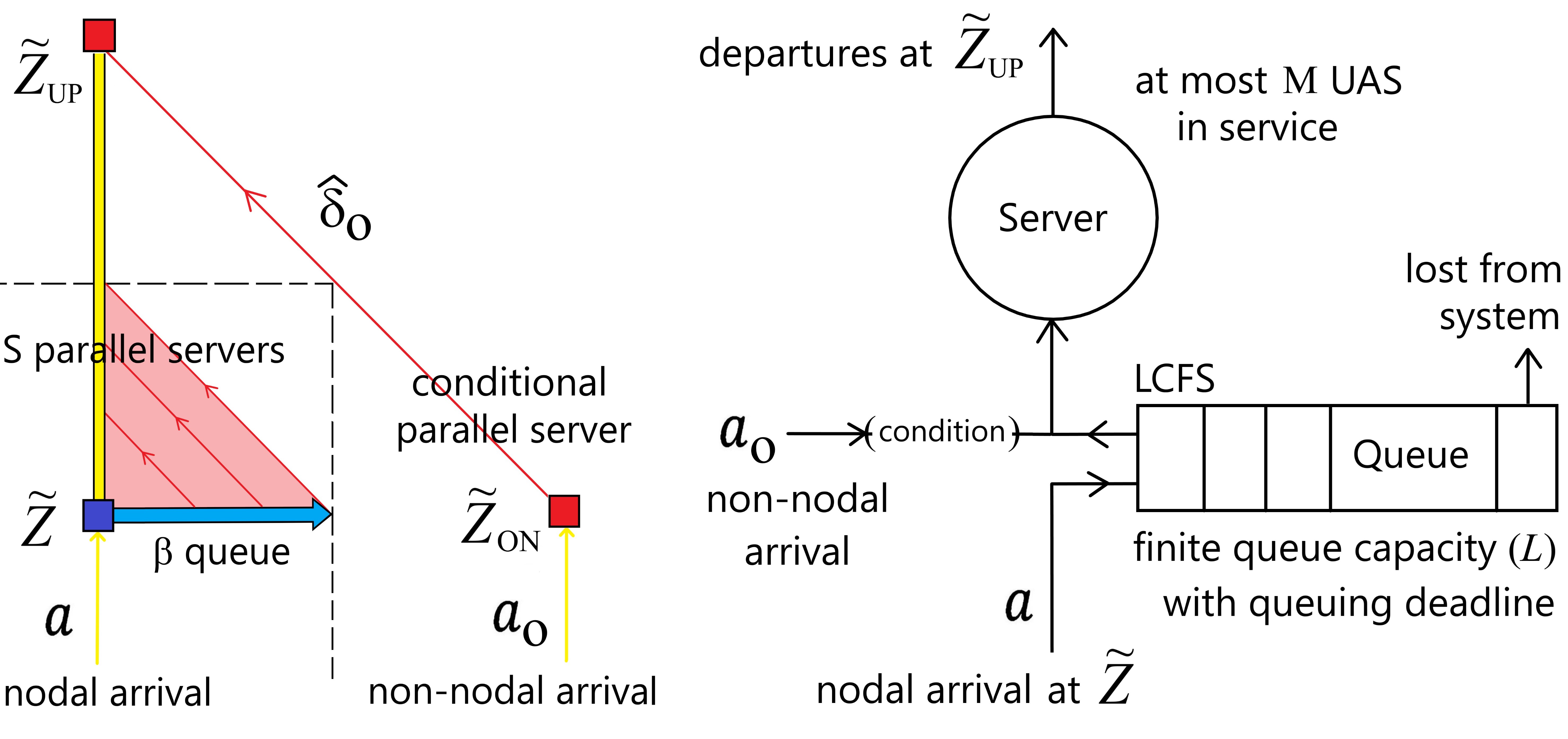
Let be random variables such that at time slot , gives the total number of UAS currently in the queue that have queued for no more than slots since entering the queue. implies that an arrival found the system busy in time slot and thus entered the queue and has queued for timeslot since then. gives the total number of UAS present in the queue. A UAS that has queued for slots (that is, successive transitions on ) exits the system in the next time slot. Hence, there is a queuing deadline of time slots to enter service, beyond which the UAS is lost from the system. As the queue never goes unbounded, the limiting probability distributions as exist.
The UAS preference decreases with each queued time slot. A UAS that has queued for the least number of slots has the highest preference. Hence, by Rule 3, if the system is idle ( is uncongested), then UAS with the highest preference enters service. This is fundamentally the Last Come, First Serve (LCFS) discipline. The following dynamical equations summarize the above queuing behavior when the system is busy and idle.
If the system is busy () then
| (14) | |||
| (15) |
If the system is idle () then following LCFS
| (16) | |||
| (17) |
where the notation . Eqn. 17 states that when , then one UAS from the queue enters service (the one which arrived last). Hence, the number of UAS that have queued at most slots () reduces by one. When , then the arrival enters service, and the number of UAS that have queued slots by time slot would have queued slots by timeslot . The arrivals and are independent at timeslot . And,
| (18) |
The PGF can be derived using the conditional PGF of Eqns. 14-17 as,
Hence for ,
| (19) | |||
| (20) |
By recursively substituting in , we get . In the timeslot , a UAS will enter service if and only if the system is uncongested and, more importantly, there are UAS available to enter service, that is
-
1.
there is a UAS nodal arrival (that is ), or
-
2.
there are UAS in queue (that is ), or
-
3.
there is a UAS non-nodal arrival (that is ) available to descend towards under the condition that there are no UAS nodal arrival and no UAS in the queue (descend condition),
Thus, as , we have
| (21) | |||
| (22) | |||
| (23) |
where is referred to as steady-state descend probability that a UAS at node would descend into zone and is the probability that a UAS is available to enter service in a given time slot. The PGF of the descend probability distribution is denoted by .
Eqn. 23 is the feedback relation that captures congestion being responsible for UAS entering the Stream 0 queue. Substituting Eqn. 23 in Eqn. 13, we get a polynomial equation in . There is an indeterminate term () in Eqn. 20, which we take advantage of using Rouché’s theorem. Knowing the steady state exists and , according to Rouché’s theorem [29, 28], the roots of the denominator of Eqn. 20 are also roots of the numerator, which leads to pole-zero cancellations and the polynomial in having a unique zero in . The polynomial equation is solved numerically for . Substituting in , we get respective probabilities.
Note that the congestion definition in Eqn. 13 is defined solely on UAS being in the service or not. However, it does not account for when these UAS have entered service. It would be misleading to assume no correlation between the time instances the UAS enters service, as this affects the congestion period duration. For example, consider and service time . If a UAS enters service in timeslot followed by another UAS entering service in timeslot . As UAS are in service, the is congested in time slot , and it remains congested for the next timeslots. Instead, if the second UAS had entered service in timeslot , then the turns congested in time slot , but it remains congested only for the next timeslot. We introduce the above correlation by modeling congestion as a Markov modulated on/off regular process (MMRP) [30].
IV-A1 Markov-modulated regular process
An MMRP (shown in Fig. 15(a)) is a two-state Markov chain, where the state of the Markov chain depends only on the state of a two-state background process. Here, is the Markov state, with and being the probability that is congested and uncongested, respectively. The number of UAS () present in service is the background process with two states and . If then and if then . Let is the transition probability that if uncongested in timeslot turns congested in timeslot , and is the transition probability that if congested in timeslot turns uncongested in timeslot , respectively. is the transition probability that remains congested and is the transition probability that it remains uncongested. Let denote the steady-state probability that a UAS is available to enter service (including exogenous arrivals) in any given time slot.
In a time interval of timeslots, if UAS were available to enter service, then the would be congested in the th timeslot. The would remain congested if and only if no UAS are departing in the next time slot, that is, there are no UAS that have received slots of service as shown in Fig. 15(b). This behavior is summarized in Eqn 24.
| (24) |
In the timeslot interval, if no more than UAS were available to enter service, then the would be uncongested in the th timeslot. Given uncongested, the would turn congested in the next time slot if UAS are already in service, no UAS are departing, and at least one UAS is available to enter the service (shown in Fig. 15(b)). This behavior is summarized in Eqn 25.
| (25) |
The Markov modulated congestion probability as derived in [30] is given by,
| (26) |
IV-A2 Markov modulated Bernoulli process (MMBP)
In a given timeslot, whether a UAS would enter service or not is correlated to the being congested and UAS being available. If , then . However, when , if UAS is available then with probability else with probability . is an MMBP, which refers to the Markov chain that generates a sequence of zeros when the background process is in one state and generates a Bernoulli process when the background process is in the second state (as shown in Fig. 16). Here, is the two-state Markov chain with being the background process. The Markov modulated probability that a UAS would enter service as derived in [30] is given by
| (27) |
The average number of UAS present in the service and the queue can be obtained by substituting and in and and computing and , respectively. The sum of the average number of UAS in the queue and the service is the expected number of UAS present in zone .
IV-A3 Queue overflow
The UAS that have queued for slots are lost from the queue and become non-nodal arrivals to the Stream queueing system. The steady-state probability that in timeslot , a UAS queuing would be lost from the system is called Queue overflow probability . Let be a random variable that there exists a UAS that has queued for slots in time slot .
| (28) |
As , we have,
| (29) | |||
| (30) |
Summing Eqns. 29-30 for and simplifying we get,
| (31) | |||
| (32) | |||
| (33) |
The UAS corresponding to has the least preference () amongst other UAS present in the queue, including the nodal arrival . If the is uncongested in time slot and there are higher UAS, then the UAS that has last arrived would enter service, forcing the UAS corresponding to to queue an additional slot. This UAS would have queued for slots and hence is lost from the system. When turns congested, under steady-state, the fraction of UAS arrivals that entered the queue but failed to enter service when was uncongested are lost during the congestion period. Thus, the Queue overflow probability is given by,
| (34) |
Following Rule 7, the steady-state probability distribution of the non-nodal arrivals for the neighboring Stream queuing system is given by
| (35) |
The non-nodal arrival probability distribution for neighboring Stream system is given by
| (36) |
IV-B Stream queuing system
The schematic for the Stream queuing system is shown in Fig. 17. A Stream queuing system has nodal arrivals and non-nodal arrivals . These arrivals are departures and overflows from the preceding systems. Assume that the PGF of these arrivals has already been computed. Let be a random variable such that if a nodal arrival in time slot would descend to zone and is otherwise. Corresponding descend probability and PGF are also known. is dependent on the arrivals and UAS queuing in the system (refer Eqn. 21). The non-nodal arrival on finding the system busy would enter the queue. The nodal arrival on finding the system busy and descend condition unsatisfied would enter the queue.
Let be random variables such that at time slot , gives the total number of UAS currently in the queue that have queued for no more than slots since entering the queue. are respective PGFs. is the total number of UAS queuing in the queue. The non-nodal arrival on finding zone congested for successive slots would enter the node . Thus, for UAS queuing in the queue, there is a slot queuing deadline to enter service, beyond which these UAS are lost from the queue. The UAS that are lost from the queue re-enter the system via node . Hence, these UAS are also treated as nodal arrivals to the system with PGF . If there are simultaneous and nodal arrivals in timeslot , then there is conflict at node . In conflict, the nodal arrival has the highest preference and enters service. Whereas the non-nodal arrival and the UAS queuing in queue are forced to queue an additional slot. In timeslots with no conflict, the UAS in the queue that has queued for the least number of slots has the highest preference and enters service. This is nothing but the LCFS discipline.
Let be a random variable that there exists a UAS that has queued for slots in queue in time slot . When is uncongested, the UAS corresponding to is lost from the system if,
-
1.
there is a conflict at node or
-
2.
there are no conflicts at node , but there are non-nodals arrivals or UAS in queue () that have higher preference than UAS .
When turns congested, then under steady-state, the fraction of UAS arrivals that entered the queue but failed to enter service when was uncongested are lost during the congestion period. The above behavior is similar to that of Stream queue. Thus, similar to Eqns. 33-34, the PGF of nodal arrivals is given as follows.
| (37) | ||||
| (38) | ||||
| (39) |
where is a pessimistic probability of conflict in timeslot .
| (40) | ||||
| (41) |
The LCFS dynamic equations for UAS queuing in the queue are as follows. If the system is busy () or there is a conflict () then
| (42) | |||
| (43) |
If the system is idle () and there is no conflict ( or ) then
| (44) | |||
| (45) |
Eqns. 42-45 are similar to Eqns. 14-17. Thus, for the queue can be derived using the conditional PGF as,
| (46) | |||
| (47) |
By recursively substituting in , we get the PGF . The nodal arrivals and that fail to enter service in time slot would enter the queue in the next time slot. Let be random variables such that at time slot , give the total number of UAS currently in the queue, that have queued for no more than slots since entering the queue. are respective PGFs. is the total number of UAS queuing in the queue. The queuing behavior of the queue when the system is busy or idle, when the descend condition is satisfied or not, and when there is a conflict at node or not can be summarized in the following eight scenarios. Note that and are independent at timeslot . For ,
-
1.
When there is a conflict () due to simultaneous and arrivals and the descend condition is satisfied () with probability , then by rule 5 the arrival enters service and by rule 6 the descends to zone. No arrival enters the queue. Irrespective of whether the system is busy or not and whether UAS are present in the queue or not, the UAS present in the queue are forced to queue an additional slot.
| (48) | ||||
| (49) |
-
2.
If there is a conflict () but the descend condition is not satisfied () with probability , then the arrival would enter service and would enter queue.
| (50) | ||||
| (51) |
-
3.
If either the system is busy () or idle () with UAS having higher preference being present ( or ) with probability then the UAS present in queue do not enter service.
(52) -
(a)
If there is no conflict because and with probability , then the arrival would enter the queue.
(53) (54) -
(b)
If there is no conflict because , and
-
i.
if descend condition is satisfied () with probability then no UAS will enter the queue.
(55) (56) -
ii.
If the descend condition is not satisfied () with probability , then the arrival will enter the queue.
(57) (58)
-
i.
-
(a)
-
4.
If the system is idle () and there are no UAS with higher preference ( , ) with probability then
(59) -
(a)
If there is no conflict because , with probability , then enters service. No UAS enters the queue.
(60) (61) -
(b)
If there is no conflict because , and
-
i.
if the descend condition is satisfied () with probability , then descends to . No UAS enters the queue. Following LCFS discipline, the UAS in the queue that has arrived last enters service.
(62) (63) -
ii.
If the descend condition is not satisfied () with probability , then the arrival or the UAS that has arrived last enters service
(64) (65)
-
i.
-
(a)
where can be obtained from Eqn. 18 and can be obtained by substituting in Eqn. 18. The PGF can be obtained by summing the above conditional PGFs in Eqns. 48-65 using the total probability theorem. By recursively substituting in , we get . In timeslot , a UAS will enter service if there is conflict, otherwise if and only if the system is idle, and more importantly, if there are UAS available to enter service, that is,
-
1.
there is a non-nodal arrival () or,
-
2.
there are UAS in queue () or,
-
3.
there is a nodal arrival ( or , ) or,
-
4.
there are UAS in queue ()
-
5.
there is a non-nodal arrival () that descends towards when descend condition is satisfied.
The probability that a UAS will enter the service is given by,
| (66) | |||
| (67) | |||
| (68) |
where is the descend probability that a non-nodal arrival at node would descend into zone and is the probability that a UAS is available to enter service in the given time slot. Note is the descend probability that the nodal arrival at node will not descend to zone.
The Eqn. 68 is the feedback relation that captures congestion responsible for UAS queuing in a Stream queue. Substituting Eqns. 40-41 in Eqn. 68 and simplifying for , we get as a function of . Substituting Eqn. 68 in Eqn. 13, we get a polynomial equation in . Numerically solving the polynomial equation for zeros, we get the congestion probability . Substituting in , , and we get respective probabilities.
As is an MMRP and is an MMBP, the respective Markov modulated probabilities and are given by Eqns. 26- 27. The average number of UAS present in the service and queue of Stream queuing system can be obtained by substituting and in , and and computing , and , respectively.
The UAS that have queued for slots in the queue are lost from the queuing system and become non-nodal arrivals for the queuing system. If the is uncongested in time slot , but there are UAS with higher preference present (that is when there is a conflict or or or when descend condition is unsatisfied or ), then in the next timeslot, the UAS corresponding to is lost from the system. When ZUP turns congested, under steady-state, the fraction of nodal arrivals and non-nodal arrivals queueing in queue that entered the queue, but failed to enter service when ZUP was uncongested are lost during the congestion period. The steady-state queue overflow probability for the queuing system is given by,
| (69) | |||
| (70) |
The PGF for the steady-state probability distribution of the non-nodal arrivals for the neighboring queuing system is given by
| (71) |
IV-C Service departures
Knowing congestion probability , the PGF of the probability distribution that UAS would depart the queuing system after receiving service is given by Eqn. 72. The UAS departures from the system are nodal arrivals for its neighboring upstream system given by
| (72) |
The algorithmic procedure for estimating the expected spread of UAS traffic in the finite grid ; for a given geometrically distributed request rate at the source is as follows.
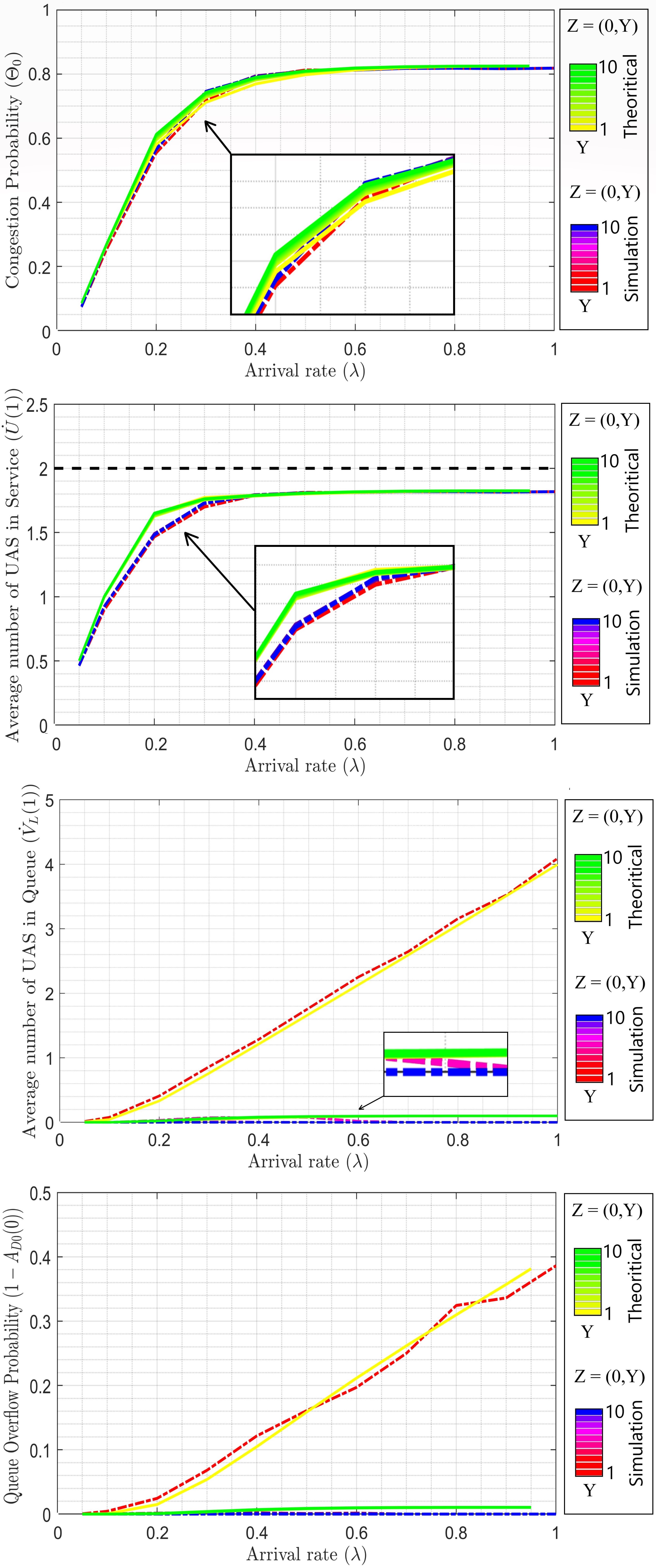
V Theoretical and Simulation Results
Consider the workspace enclosing a source-destination pair at altitude in the urban environment. The source is at , where for every request received, a UAS is deployed to deliver the payload at the paired destination. The time axis is discretized into time slots. We assume one or no request is received in any given time slot. The average rate at which the requests are received, analogously the arrival rate at which the UAS would be deployed at source, varies between average number of UAS per timeslot. For simulation, a horizontal cross-section of the workspace stretching between along axis, along axis and intersecting a static obstacle at the given altitude is considered. The UAS is enclosed in a virtual disk of safety radius . The cross-section is tessellated into cells of dimension . The UAS transitions with cell per time slot nominal velocity. The cell dimensions are large enough that there is no breach in the UAS periphery amongst UAS transitioning in respective cell neighborhoods (shown in Fig. 18). The UAS has a slot look-ahead time window, allowing it to predict where other UAS would be in the next . Assume that the UTM has prescribed a nominal path between source-destination such that in the cross-section, the set of cells through which the axis passes is the nominal segment. The cell enclosing the source is the start cell for the nominal segment. The zones are defined with edge length cells, and the finite grid (comprising streams and levels) is constructed centered on the nominal segment.
Every UAS deployed at the source follows the proposed congestion mitigation strategy. The simulation is run until around UAS are deployed at the source. The congestion
probability and expected number of UAS present in the zone are numerically computed by solving Eqn. 13 using MATLAB symbolic math toolbox. The theoretical results are validated with the average values of the UAS simulation data.
![[Uncaptioned image]](/html/2405.20972/assets/Fig_18.jpg)
Figure 19 shows snapshots of UAS distributedly employing the proposed rule-based congestion mitigation strategy. When every UAS in the source-destination traffic stream follows the proposed strategy, Fig. 20-22 show that the emerging traffic pattern closely resembles a parallel air corridor network with the number of air corridors adapting to the arrival rate 111The simulation videos have been uploaded in the following link https://youtu.be/Yk1vY6nynHg. The emergence of parallel air corridors is a consequence of the proposed strategy and UTM has no role in it nor there is any scheduling policy in place. It may be observed that in any zone no more than UAS are present, thus assuring increased UAS intrinsic safety. The above figures also demonstrate the variation in the number of active corridors, also referred to as traffic stream spread as a function of the arrival rate () and the UTM design parameters (). As the arrival rate increases or decreases, the congestion frequency and duration in the inner stream zones increases, hence more UAS shift onto outer streams, resulting in increased traffic spread. When we have denser traffic flow on the left of the nominal segment and vice versa.
When the arrival rate is small, in the lower levels the UAS inter-separation distances (depend only on arrival) are large. Hence the congestion duration is small (refer Fig. 23a). However in the higher levels, when a zone in the inner stream turns uncongested, the UAS in outer streams descend onto the inner stream (UAS marked 1 in snapshot 8 of Fig. 19). Thus, reducing UAS inter-separation distances, and resulting in longer congestion durations (refer Fig. 23b). In the zone, when , a UAS is available to enter every timeslot the zone turns uncongested (refer Fig. 23c). Thus, the zone remains congested for timeslots. For example, when and , the zone is congested for timeslots and hence the congestion probability (as validated in the plot of Fig. 24, when ). The rearrangement of UAS in the traffic stream happens such that beyond a certain level, we observe no UAS moving outward and no UAS descending inward.
![[Uncaptioned image]](/html/2405.20972/assets/Fig_19.jpg)
The same is validated in Fig. 24, the average number of UAS in the queue (that is UAS moving outward), and the queue overflow is nearly zero for Level and above zones. In the congestion probability plot, when , there is no congestion, so no UAS shifts onto outer streams and hence no UAS available to descend. The inter-separation distances depend only on arrival. Thus, the congestion duration remains unaffected as levels increase. When , there is congestion but the duration is small. There are UAS that descend and increase the congestion duration in the higher levels. However, on average the increase is not significant as with the increase in the congestion duration, the probability that a UAS would descend decreases. When , the congestion durations are long enough that most of the UAS arriving in the lower levels shift onto outer streams. However, these UAS rarely descend (refer Fig. 25b). Hence again the congestion duration remains unaffected as the level increases. Thus as and as the congestion probabilities of all zones converge.
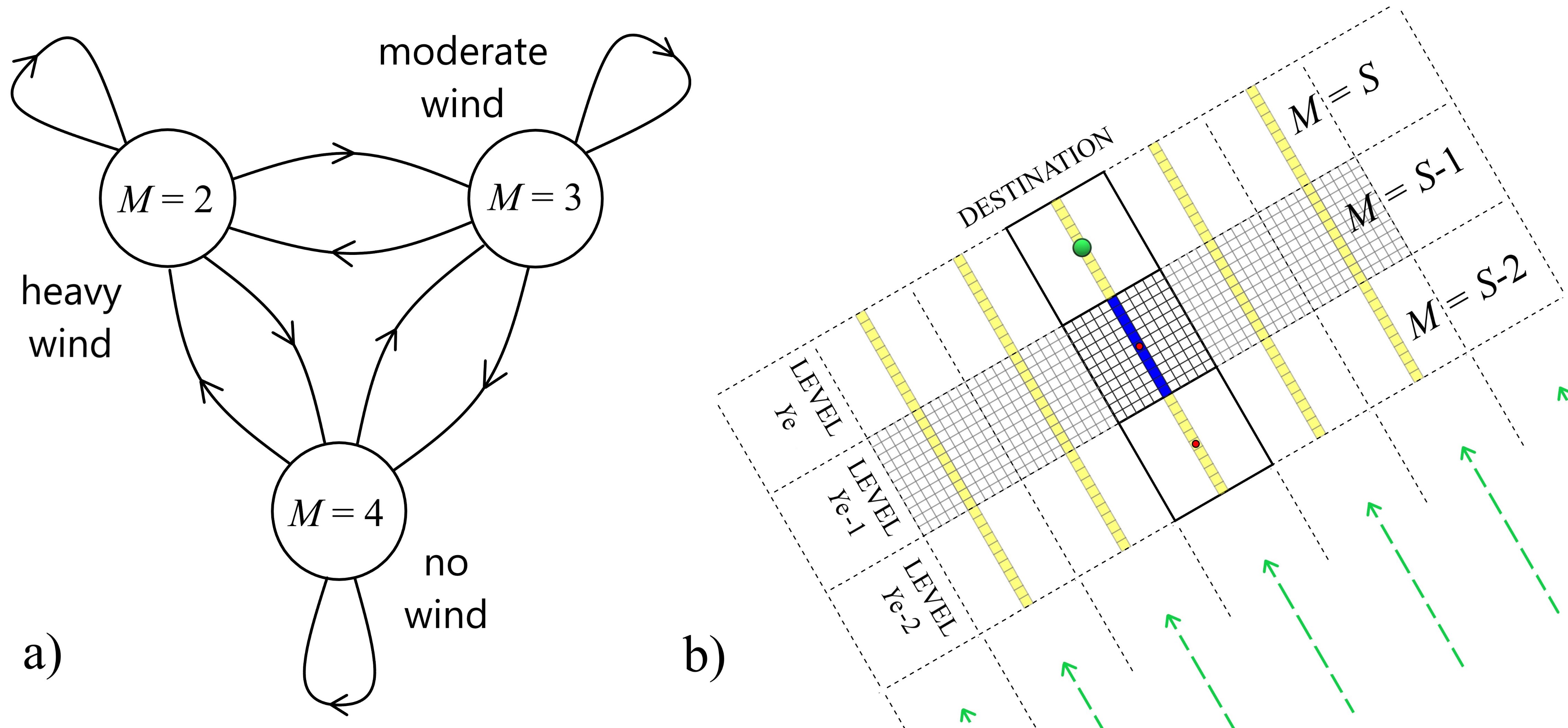
Unlike arrival rate which cannot be controlled, the UTM can take strategic decisions for parameters and . Figure 26 shows Rule 7 being employed by UAS in the presence of a static obstacle, due to which the UAS circumnavigate the obstacle. Instead, the UTM could choose an such that the traffic spread (shown in Fig. 21) would not pass through the static obstacle. In general, the traffic flow in the urban airspace is weather-dependent. As per UAS safety standards, the allowable congestion in a region is constrained on wind conditions. As in [19], the weather is modeled as a first-order Markov chain with zero, moderate, and heavy wind as states. The UTM may associate each state with a value (shown in Fig. 27a). Corresponding to prevailing wind condition, the UTM communicates respective value with the UAS. The UAS accordingly adapt ensuring no more than UAS are present in any zone, as shown in Fig. 22. Another use case for changing would be at the destination. must be gradually incremented over the levels (as shown in Fig. 27b) so that when in the final level containing the destination node, all UAS would enter the destination.
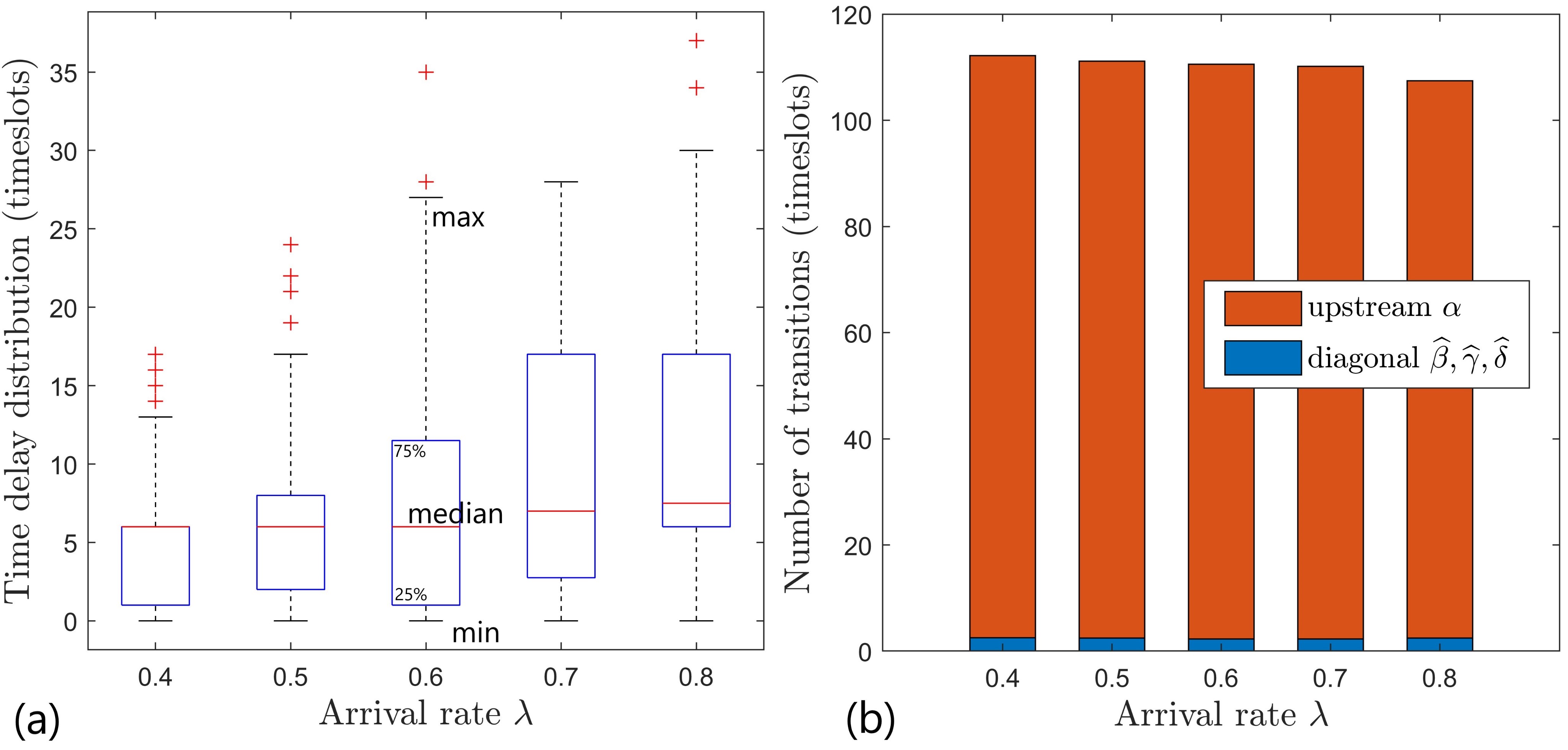
When executing a diagonal transition, to travel 1 unit distance in the upstream direction the UAS needs times higher velocity than when executing an upstream transition. Thus, diagonal transitions are energy-intensive maneuvers. However, as shown in Fig. 25b, the number of diagonal transitions executed is low and mostly confined to the lower levels.
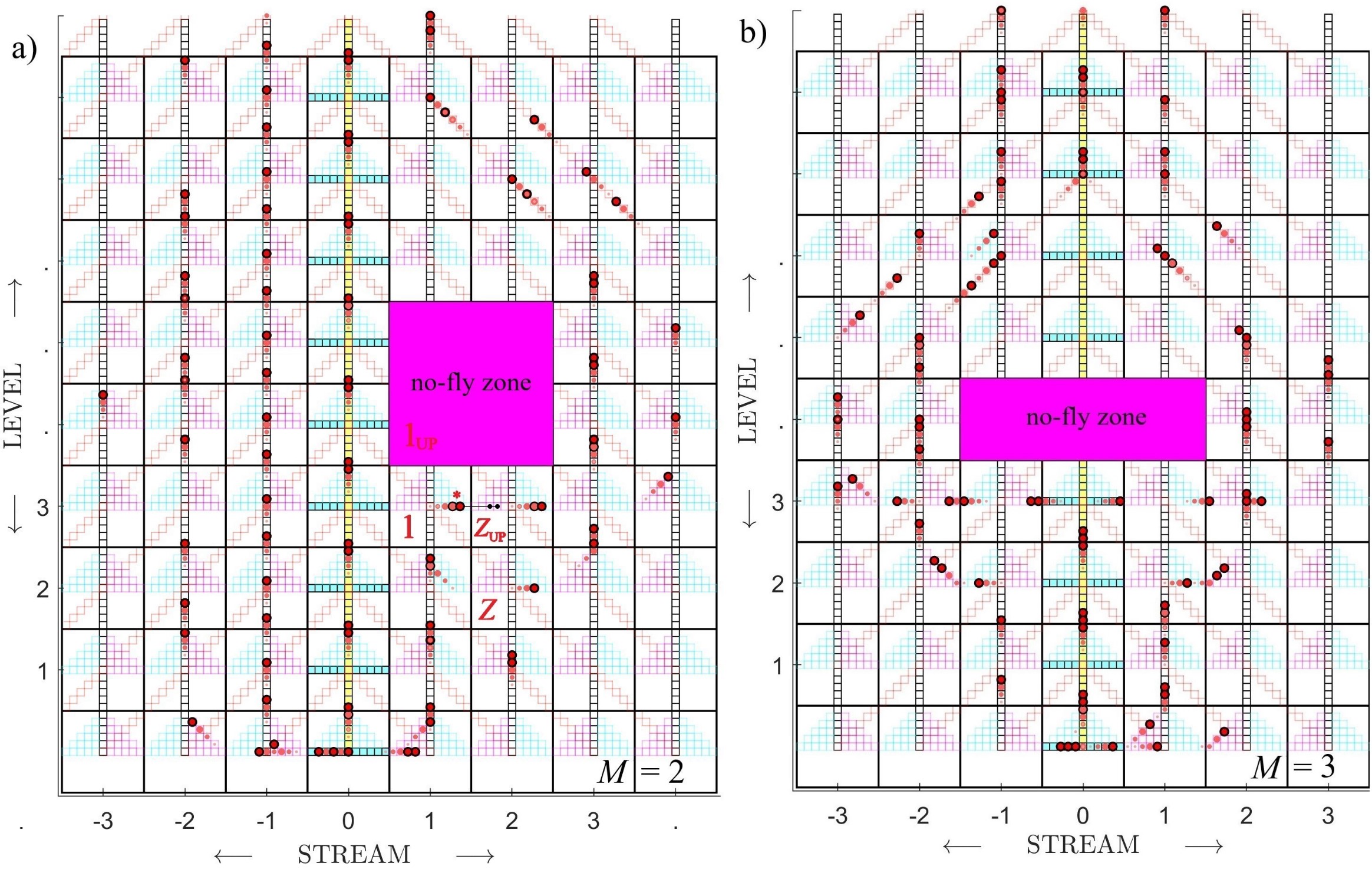
In Fig. 26a, the UAS marked in zone always perceive zone to be congested. These UAS would certainly enter zone . The respective look-ahead positions can be determined and hence these UAS are included in Definition 2. Thus, UAS in zone are affected by UAS .
For any given and , the UTM could estimate the expected traffic spread, and the expected number of UAS in the zone beforehand using the queueing models discussed in section IV. Based on these estimates the UTM could decide on the look-ahead window to define the zone and then decide on the parameters and for the appropriate use case. Fig 28-29 provide validation for theoretical estimates obtained from the queuing models.
When , we have an arrival every timeslot in the zone. As mentioned before, the zone would be congested for timeslots, and hence congestion probability is . The same can be verified in Fig. 28a for different values of . The average number of UAS in service never exceeds . The UAS queuing would be in either of the two queues each of capacity , with probability and (). Hence, the average number of UAS in the queue never exceeds . In Fig. 28-29 for zone , there maybe UAS queuing in both and queues. Hence, the average number of UAS queueing never exceeds . Only a fraction of the UAS arrivals to zone are lost from the queue to become non-nodal arrivals for zones. For a given arrival rate , the zone has higher congestion probability than zone as less number of UAS are available in zones to enter service. For the same reason, zones and have greater than outer neighboring and zones, respectively. When , we have equal in zones. When all UAS lost from become non-nodal arrivals to else only fraction of UAS lost become non-nodal arrivals. For any given , as more number of UAS are available to enter service when , hence in we have more number of UAS in service, resulting in increased congestion, and more number of UAS in the queue when compared to .
V-A Presence of exogenous traffic stream
Following Assumptions 1-3, an exogenous traffic stream perpendicularly intersecting the nominal segment at Level 2 is considered (refer Fig. 30a). The exogenous UAS arrival rate is . The expected number of exogenous UAS in the Level zones is . must be greater than for UAS to cross the exogenous traffic stream, hence is chosen to be . The exogenous UAS transitions with cell per time slot nominal velocity. The exogenous UAS do not follow the proposed mitigation strategy and are hence unaffected by congestion in the zone. However, the exogenous UAS contributes to congestion. When or more than look-ahead positions (exogenous UAS included) are present in a zone, then the UAS laterally transitions to avoid such zone (as shown in snapshot 1 of Fig. 30a). Unlike in the presence of a static obstacle, where it is certain that a UAS would always laterally transition every timeslot when in path, in the presence of an exogenous stream when the UAS would laterally transition is uncertain (congestion-dependent) and thus are not included in Definition . This results in the UAS transitioning laterally and those transitioning upstream experiencing conflicts (as shown in snapshot 1-2 of Fig. 30a). A conflict among UAS belonging to the same stream is referred to as internal conflict. A conflict between a UAS and an exogenous UAS is referred to as exogenous conflict. Though conflicts occur, the congestion mitigation strategy guarantees no more than conflicts in any zone, that is UAS intrinsic safety is improved. Further, the mitigation strategy helps reduce the total number of conflicts in the stream (as shown in Fig. 30b). These advantages come at the expense of additional time delay in the UAS path and energy cost proportional to the number of diagonal transitions (refer Fig. 30b. Here, the total number of upstream and diagonal transitions executed to reach Level zone is ). Note that the additional cost is insignificant when computed over the entire flight path. Depending on the inter-separation distance distribution between the exogenous UAS, the traffic spread may increase or decrease as shown in snapshots 3-4 of Fig. 30a. However, the queueing models can be used to estimate the expected traffic spread as validated in Fig. 30c.
VI Conclusion
In this paper, we present a heading-constrained airspace design for the altitude-layered urban airspace and propose a novel preference-based distributed congestion mitigation strategy. The proposed strategy offers a unified framework for handling contingencies such as congestion in the urban airspace, conflicts among exogenous UAS traffic streams, and static obstacle avoidance. The advantages of the proposed approach are many-fold. The airspace design is the responsibility of UTM which could be done offline and the UTM parameters could be communicated to the UAS as needed. The strategy is decentralized with individual UAS being responsible for mitigating congestion and minimal role played by UTM. Hence, the strategy is scalable to the rapidly growing number of UAS. The strategy improves UAS intrinsic safety by guaranteeing no more than UAS are present in any zone, also reducing the number of UAS conflicts. However, this comes at the expense of a minimal time delay and energy costs introduced in the UAS flight path associated with lateral and diagonal maneuvers. The emerging traffic behavior when every UAS employs the proposed strategy closely resembles a parallel air-corridor network, with the number of active air-corridors (referred to as traffic stream spread) adapting to the UAS demand. The UAS traffic is directional, thus no compromise on the UTM throughput. The paper also presents queueing theory models for estimating the expected traffic spread for any given UAS demand. The estimates help the UTM reserve the airspace beforehand for any foreseen congestion. Extending the above strategy to the general scenario where more than two exogenous UAS traffic streams intersect (may not be perpendicular) and affect each other would be the future avenue of this work. Further, proposing a probabilistic confidence definition for congestion instead of the present deterministic Definition 1 would help further reduce the internal conflicts. There may be other factors that affect the UAS preference to avoid or enter a congested region, that can be incorporated into the above strategy.
Acknowledgment
The research reported here was funded by the Commonwealth Scholarship Commission and the Foreign, Commonwealth and Development Office in the UK. Sajid Ahamed is grateful for their support. All views expressed here are those of the author(s) not the funding body.
References
- [1] P. Kopardekar, J. Rios, T. Prevot, M. Johnson, J. Jung, and J. E. Robinson, “Unmanned aircraft system traffic management (UTM) concept of operations,” AIAA Aviation Forum, 2016.
- [2] C. P. Catapult, “Enabling UTM in UK,” Connected Places Catapult, London, UK, 2020, (Accessed on 24 September 2023). [Online]. Available: https://www.suasnews.com/wp-content/uploads/2020/05/Connected-Places-Catapult-report-Enabling-UTM-in-the-UK-2.pdf
- [3] K. Balakrishnan, J. Polastre, J. Mooberry, R. Golding, and P. Sachs, “Blueprint for the sky: The roadmap for the safe integration of autonomous aircraft,” Airbus UTM, San Francisco, CA, 2018, (Accessed on 24 September 2023). [Online]. Available: https://storage.googleapis.com/blueprint/Airbus_UTM_Blueprint.pdf
- [4] B. Pang, W. Dai, T. Ra, and K. H. Low, “A concept of airspace configuration and operational rules for UAS in current airspace,” in 2020 AIAA/IEEE 39th Digital Avionics Systems Conference (DASC). IEEE, 2020, pp. 1–9.
- [5] L. A. Tony, A. Ratnoo, and D. Ghose, “Lane geometry, compliance levels, and adaptive geo-fencing in CORRIDRONE architecture for urban mobility,” in 2021 International Conference on Unmanned Aircraft Systems (ICUAS). IEEE, 2021, pp. 1611–1617.
- [6] J. M. Hoekstra, J. Ellerbroek, E. Sunil, and J. Maas, “Geovectoring: reducing traffic complexity to increase the capacity of UAV airspace,” in International conference for research in air transportation, Barcelona, Spain, 2018.
- [7] M. Doole, J. Ellerbroek, V. L. Knoop, and J. M. Hoekstra, “Constrained urban airspace design for large-scale drone-based delivery traffic,” Aerospace, vol. 8, no. 2, p. 38, 2021.
- [8] B. Li, S. Wang, C. Ge, Q. Fan, and C. Temuer, “Bi-level intelligent dynamic path planning for an UAV in low-altitude complex urban environment,” Transactions of the Institute of Measurement and Control, p. 01423312231167200, 2023.
- [9] S. A. M. Abdul, K. S. Prakash, S. Jana, and D. Ghose, “Numerical potential fields based multi-stage path planning for UTM in dense non-segregated airspace,” Journal of Intelligent & Robotic Systems, vol. 109, no. 1, pp. 1–30, 2023.
- [10] L. Agnel Tony, D. Ghose, and A. Chakravarthy, “Unmanned aerial vehicle mid-air collision detection and resolution using avoidance maps,” Journal of Aerospace Information Systems, vol. 18, no. 8, pp. 506–529, 2021.
- [11] D. Sacharny, T. C. Henderson, and V. V. Marston, “Lane-based large-scale UAS traffic management,” IEEE Transactions on Intelligent Transportation Systems, vol. 23, no. 10, pp. 18 835–18 844, 2022.
- [12] S. R. Nagrare, A. Ratnoo, and D. Ghose, “Intersection planning for multilane unmanned aerial vehicle traffic management,” Journal of Aerospace Information Systems, vol. 21, no. 3, pp. 216–233, 2024.
- [13] L. Watkins, N. Sarfaraz, S. Zanlongo, J. Silbermann, T. Young, and R. Sleight, “An investigative study into an autonomous UAS traffic management system for congested airspace safety,” in 2021 IEEE International Conference on Communications Workshops (ICC Workshops). IEEE, 2021, pp. 1–6.
- [14] L. Sedov, V. Polishchuk, and V. Bulusu, “Decentralized self-propagating ground delay for UTM: Capitalizing on domino effect,” in 2017 Integrated Communications, Navigation and Surveillance Conference (ICNS). IEEE, 2017, pp. 6C1–1.
- [15] M. J. Aarts, J. Ellerbroek, and V. L. Knoop, “Capacity of a constrained urban airspace: Influencing factors, analytical modelling and simulations,” Transportation Research Part C: Emerging Technologies, vol. 152, p. 104173, 2023.
- [16] E. Sunil, J. Ellerbroek, J. M. Hoekstra, and J. Maas, “Three-dimensional conflict count models for unstructured and layered airspace designs,” Transportation Research Part C: Emerging Technologies, vol. 95, pp. 295–319, 2018.
- [17] S. Lee, D. Hong, J. Kim, D. Baek, and N. Chang, “Congestion-aware multi-drone delivery routing framework,” IEEE Transactions on Vehicular Technology, vol. 71, no. 9, pp. 9384–9396, 2022.
- [18] M. Egorov, V. Kuroda, and P. Sachs, “Encounter aware flight planning in the unmanned airspace,” in 2019 Integrated Communications, Navigation and Surveillance Conference (ICNS). IEEE, 2019, pp. 1–15.
- [19] J. Zhou, L. Jin, X. Wang, and D. Sun, “Resilient UAV traffic congestion control using fluid queuing models,” IEEE Transactions on Intelligent Transportation Systems, vol. 22, no. 12, pp. 7561–7572, 2020.
- [20] M. Gharibi, Z. Gharibi, R. Boutaba, and S. L. Waslander, “A density-based and lane-free microscopic traffic flow model applied to unmanned aerial vehicles,” Drones, vol. 5, no. 4, p. 116, 2021.
- [21] Z. Wang, D. Delahaye, J.-L. Farges, and S. Alam, “Air traffic assignment for intensive urban air mobility operations,” Journal of Aerospace Information Systems, vol. 18, no. 11, pp. 860–875, 2021.
- [22] L. Agnel Tony, D. Ghose, and A. Chakravarthy, “Correlated-equilibrium-based unmanned aerial vehicle conflict resolution,” Journal of Aerospace Information Systems, vol. 19, no. 4, pp. 283–304, 2022.
- [23] J. Yang, D. Yin, L. Shen, Q. Cheng, and X. Xie, “Cooperative deconflicting heading maneuvers applied to unmanned aerial vehicles in non-segregated airspace,” Journal of Intelligent & Robotic Systems, vol. 92, pp. 187–201, 2018.
- [24] K. Zeghal, “A review of different approaches based on force fields for airborne conflict resolution,” in Guidance, Navigation, and Control Conference and Exhibit, 1998, p. 4240.
- [25] P. Gao, S. Wittevrongel, and H. Bruneel, “Discrete-time multiserver queues with geometric service times,” Computers & Operations Research, vol. 31, no. 1, pp. 81–99, 2004.
- [26] I. Atencia and A. V. Pechinkin, “A discrete-time queueing system with optional LCFS discipline,” Annals of Operations Research, vol. 202, pp. 3–17, 2013.
- [27] S. Wittevrongel and H. Bruneel, “Discrete-time queues with correlated arrivals and constant service times,” Computers & Operations Research, vol. 26, no. 2, pp. 93–108, 1999.
- [28] H. Bruneel and I. Wuyts, “Analysis of discrete-time multiserver queueing models with constant service times,” Operations Research Letters, vol. 15, no. 5, pp. 231–236, 1994.
- [29] H. Kobayashi and A. Konheim, “Queueing models for computer communications system analysis,” IEEE Transactions on Communications, vol. 25, no. 1, pp. 2–29, 1977.
- [30] J. Smiesko, M. Kontsek, and K. Bachrata, “Markov-modulated on–off processes in IP traffic modeling,” Mathematics, vol. 11, no. 14, p. 3089, 2023.
| Sajid Ahamed M A is currently a Ph.D. student at the Department of Aerospace Engineering, Indian Institute of Science, Bengaluru. He received his Master’s degree in Control System Engineering from the Indian Institute of Space Science and Technology, Trivandrum in 2020. He received his Bachelor’s degree in Electrical and Electronics Engineering from Jawaharlal Nehru Technological University, Hyderabad in 2015. His research interests include aerial robotics, autonomous motion planning, queueing and game theory for Unmanned Aircraft Systems Traffic Management (UTM). |
| Prathush P Menon is an Associate Professor of Control and Autonomy at the Department of Engineering in the Faculty of Environment, Science, and Economy. He leads the research activities in the Cooperative Robotics and Autonomous NEtworks (CRANE) lab. He received a Ph.D. in control engineering from the Department of Engineering, University of Leicester, UK, in 2007. From 2007 to 2008, He worked at University of Leicester as a European Space Agency (ESA) funded post-doctoral research associate (PDRA), and then as lecturer. He joined the College of Engineering, Mathematics and Physical Sciences, University of Exeter, in 2010. |
| Debasish Ghose (Senior Member, IEEE) received a Ph.D. degree from the Indian Institute of Science, Bengaluru, India, in 1990. He is currently a Professor at the Indian Institute of Science. He has been a Visiting Faculty with various universities, including the University of California at Los Angeles, Los Angeles, CA, USA. His research area is in control of autonomous and multiagent systems with applications in autonomous vehicles, large-scale systems, game-theoretical models, robotics, and computational algorithms. Dr. Ghose is a fellow of the Indian Academy of Engineering and an Associate Fellow of the American Institute of Aeronautics and Astronautics. |