Amortizing intractable inference in diffusion models
for vision, language, and control

Abstract

Diffusion models have emerged as effective distribution estimators in vision, language, and reinforcement learning, but their use as priors in downstream tasks poses an intractable posterior inference problem. This paper studies amortized sampling of the posterior over data, ${\mathbf{x}}\sim p^{\rm post}({\mathbf{x}})\propto p({\mathbf{x}})r({\mathbf{x}})$, in a model that consists of a diffusion generative model prior $p({\mathbf{x}})$ and a black-box constraint or likelihood function $r({\mathbf{x}})$. We state and prove the asymptotic correctness of a data-free learning objective, relative trajectory balance, for training a diffusion model that samples from this posterior, a problem that existing methods solve only approximately or in restricted cases. Relative trajectory balance arises from the generative flow network perspective on diffusion models, which allows the use of deep reinforcement learning techniques to improve the discovery of modes of the target distribution. Experiments illustrate the broad potential of unbiased inference of arbitrary posteriors under diffusion priors across a collection of modalities: in vision (classifier guidance), language (infilling under a discrete diffusion LLM), and multimodal data (text-to-image generation). Beyond generative modeling, we apply relative trajectory balance to the problem of continuous control with a score-based behavior prior, achieving state-of-the-art results on benchmarks in offline reinforcement learning. Code is available at this link.

1 Introduction

Diffusion models [66, 26, 70] are a powerful class of hierarchical generative models, used to model complex distributions over images [e.g., 50, 11, 62], text [e.g., 4, 12, 39, 23, 22, 42], and actions in reinforcement learning [29, 81, 31]. In each of these domains, downstream problems require sampling product distributions, where a pretrained diffusion model serves as a prior $p({\mathbf{x}})$ that is multiplied by an auxiliary constraint $r({\mathbf{x}})$. For example, if $p({\mathbf{x}})$ is a prior over images defined by a diffusion model, and $r({\mathbf{x}})=p(c\mid{\mathbf{x}})$ is the likelihood that an image ${\mathbf{x}}$ belongs to class $c$, then class-conditional image generation requires sampling from the Bayesian posterior $p({\mathbf{x}}\mid c)\propto p({\mathbf{x}})p(c\mid{\mathbf{x}})$. In offline reinforcement learning, if $\mu(a\mid s)$ is a conditional diffusion model over actions serving as a behavior policy, KL-constrained policy improvement [54, 43] requires sampling from the normalized product of $\mu(a\mid s)$ with a Boltzmann distribution defined by a $Q$-function, $\pi^{*}(a\mid s)\propto\mu(a\mid s)\exp(\beta Q(s,a))$. In language modeling, various conditional generation problems [42, 22, 28] amount to posterior sampling under a discrete diffusion model prior. Table 1 summarizes four such problems that this paper studies and in which our proposed algorithms improve upon prior work.The hierarchical nature of the generative process in diffusion models, which generate samples from $p({\mathbf{x}})$ by a deep chain of stochastic transformations, makes exact sampling from posteriors $p({\mathbf{x}})r({\mathbf{x}})$ under a black-box function $r({\mathbf{x}})$ intractable. Common solutions to this problem involve inference techniques based on linear approximations [e.g., 71, 32, 30, 10] or stochastic optimization [21, 47]. Others estimate the ‘guidance’ term – the difference in drift functions between the diffusion models sampling the prior and posterior – by training a classifier on noised data [11], but when such data is not available, one must resort to approximations or Monte Carlo estimates [e.g., 68, 13, 9], which are challenging to scale to high-dimensional problems. Reinforcement learning methods that have recently been proposed for this problem [7, 15] are biased and prone to mode collapse (Fig. 1).

Contributions.

Inspired by recent techniques in training diffusion models to sample distributions defined by unnormalized densities [87, 61, 76, 64], we propose an asymptotically unbiased training objective, called relative trajectory balance (RTB), for training diffusion models that sample from posterior distributions under a diffusion model prior (§3.1). RTB is derived from the perspective of diffusion models as continuous generative flow networks [37]. This perspective also allows us to freely leverage off-policy training, when data with high density under the posterior is available (§3.2). RTB can be applied to iterative generative processes beyond standard diffusion models: our methods generalize to discrete diffusion models and extend existing methods for autoregressive language models (§3.3).

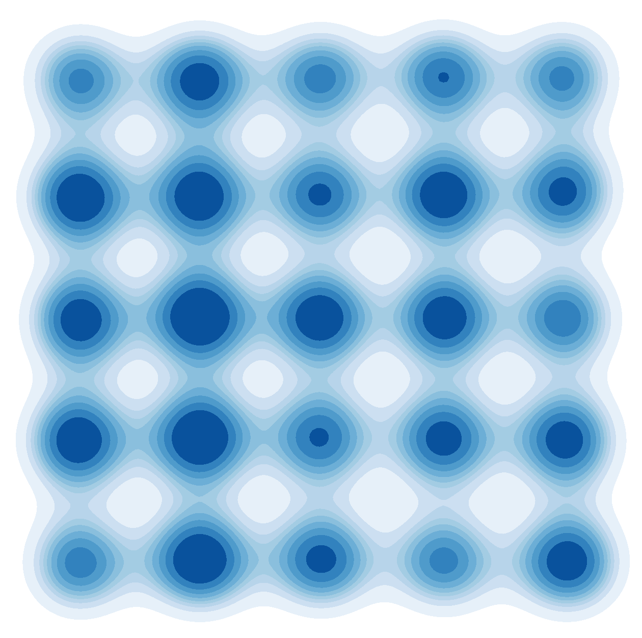
(a) Prior

(b) Posterior

(c) RTB (ours)

(d) RL (KL reg.)

(e) RL (no reg.)

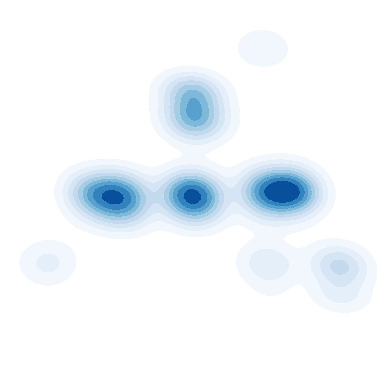
(f) CG

Figure 1: Sampling densities learned by various posterior inference methods. The prior is a diffusion model sampling a mixture of 25 Gaussians (a) and the posterior is the product of the prior with a constraint that masks all but 9 of the modes (b). Our method (RTB) samples close to the true posterior (c). RL methods with tuned KL regularization yield inaccurate inference (d), while without KL regularization, they mode-collapse (e). A classifier guidance (CG) approximation (f) results in biased outcomes. For details, see §C.

Table 1: Sources of diffusion priors and constraints.

Domain	Prior $p({\mathbf{x}})$	Constraint $r({\mathbf{x}})$	Posterior
Conditional image generation (§4.1)	Image diffusion model $p({\mathbf{x}})$	Classifier likelihood $p(c\mid{\mathbf{x}})$	Class-conditional distribution $p({\mathbf{x}}\mid c)$
Text-to-image generation (§4.2)	Text-to-image foundation model	RLHF reward model	Aligned text-to-image model
Language infilling (§4.3)	Discrete diffusion model	Autoregressive completion likelihood	Infilling distribution
Offline RL policy extraction (§4.4)	Diffusion model as behavior policy	Boltzmann dist. of $Q$-function	Optimal KL-constrained policy

Our experiments demonstrate the versatility of our approach in a variety of domains:

• In vision, we show that RTB achieves competitive classifier-guided image generation for unconditional diffusion vision priors (§4.1) and can be used to improve caption-conditioned generation under text-to-image foundation model priors (§4.2).

• In language modeling, we report strong results for infilling tasks with discrete diffusion language models (§4.3).

• Finally, we show that RTB achieves state-of-the-art results on continuous control benchmarks that leverage score-based behavior priors (§4.4).

2 Setting: Diffusion models as hierarchical generative models

A denoising diffusion model generates data ${\mathbf{x}}_{1}$ by a Markovian generative process:

$$\text{\it(noise)}\quad{\mathbf{x}}_{0}\rightarrow{\mathbf{x}}_{\Delta t}\rightarrow{\mathbf{x}}_{2\Delta t}\rightarrow\ldots\rightarrow{\mathbf{x}}_{1}={\mathbf{x}}\quad\text{\it(data)},$$ (1)

where $\Delta t=\frac{1}{T}$ and $T$ is the number of discretization steps. The initial distribution $p({\mathbf{x}}_{0})$ is fixed (typically to ${\mathcal{N}}(\bm{0},\bm{I})$) and the transition from ${\mathbf{x}}_{t-1}$ to ${\mathbf{x}}_{t}$ is modeled as a Gaussian perturbation with time-dependent variance:

$$p({\mathbf{x}}_{t+\Delta t}\mid{\mathbf{x}}_{t})={\mathcal{N}}({\mathbf{x}}_{t+\Delta t}\mid{\mathbf{x}}_{t}+u_{t}({\mathbf{x}}_{t})\Delta t,\sigma_{t}^{2}\Delta t\bm{I}).$$ (2)

The scaling of the mean and variance by $\Delta t$ is insubstantial for fixed $T$, but ensures that the diffusion process is well-defined in the limit $T\to\infty$ assuming regularity conditions on $u_{t}$ [52, 63]. The process given by (1, 2) is then identical to Euler-Maruyama integration of the stochastic differential equation (SDE) $d{\mathbf{x}}_{t}=u_{t}({\mathbf{x}}_{t})\,dt+\sigma_{t}\,d{\mathbf{w}}_{t}$.The likelihood of a denoising trajectory ${\mathbf{x}}_{0}\rightarrow{\mathbf{x}}_{\Delta t}\rightarrow\dots\rightarrow{\mathbf{x}}_{1}$ factors as

$$p({\mathbf{x}}_{0},{\mathbf{x}}_{\Delta t},\dots,{\mathbf{x}}_{1})=p({\mathbf{x}}_{0})\prod_{i=1}^{T}p({\mathbf{x}}_{i\Delta t}\mid{\mathbf{x}}_{(i-1)\Delta t})$$ (3)

and defines a marginal density over the data space:

$$p({\mathbf{x}}_{1})=\int p({\mathbf{x}}_{0},{\mathbf{x}}_{\Delta t},\dots,{\mathbf{x}}_{1})\,d{\mathbf{x}}_{0}\,d{\mathbf{x}}_{\Delta t}\ldots d{\mathbf{x}}_{1-\Delta t}.$$ (4)

A reverse-time process, ${\mathbf{x}}_{1}\rightarrow{\mathbf{x}}_{1-\Delta t}\rightarrow\dots\rightarrow{\mathbf{x}}_{0}$, with densities $q$, can be defined analogously, and similarly defines a conditional density over trajectories:

$$q({\mathbf{x}}_{0},{\mathbf{x}}_{\Delta t},\dots,{\mathbf{x}}_{1-\Delta t}\mid{\mathbf{x}}_{1})=\prod_{i=1}^{T}q({\mathbf{x}}_{(i-1)\Delta t}\mid{\mathbf{x}}_{i\Delta t}).$$ (5)

In the training of diffusion models, as discussed below, the process $q$ is typically fixed to a simple distribution (usually a discretized Ornstein-Uhlenbeck process), and the result of training is that $p$ and $q$ are close as distributions over trajectories.

Diffusion model training as divergence minimization.

Diffusion models parametrize the drift $u_{t}({\mathbf{x}}_{t})$ in (2) as a neural network $u({\mathbf{x}}_{t},t;\theta)$ with parameters $\theta$ and taking ${\mathbf{x}}_{t}$ and $t$ as input. We denote the distributions over trajectories induced by (3, 4) by $p_{\theta}$ to show their dependence on the parameter.In the most common setting, diffusion models are trained to maximize the likelihood of a dataset. In the notation above, this corresponds to assuming $q({\mathbf{x}}_{1})$ is fixed to an empirical measure (with the points of a training dataset ${\mathcal{D}}$ assumed to be i.i.d. samples from $q({\mathbf{x}}_{1})$). Training minimizes with respect to $\theta$ the divergence between the processes $q$ and $p_{\theta}$:

$$D_{\mathrm{KL}}(q({\mathbf{x}}_{0},{\mathbf{x}}_{\Delta t},\dots,{\mathbf{x}}_{1})\,\|\,p_{\theta}({\mathbf{x}}_{0},{\mathbf{x}}_{\Delta t},\dots,{\mathbf{x}}_{1}))$$ (6)

$$=D_{\mathrm{KL}}(q({\mathbf{x}}_{1})\,\|\,p_{\theta}({\mathbf{x}}_{1}))+{\mathbb{E}}_{{\mathbf{x}}_{1}\sim q({\mathbf{x}}_{1})}D_{\mathrm{KL}}(q({\mathbf{x}}_{0},{\mathbf{x}}_{\Delta t},\dots,{\mathbf{x}}_{1-\Delta t}\mid{\mathbf{x}}_{1})\,\|\,p_{\theta}({\mathbf{x}}_{0},{\mathbf{x}}_{\Delta t},\dots,{\mathbf{x}}_{1-\Delta t}\mid{\mathbf{x}}_{1}))$$

$$\geq D_{\mathrm{KL}}(q({\mathbf{x}}_{1})\,\|\,p_{\theta}({\mathbf{x}}_{1}))={\mathbb{E}}_{{\mathbf{x}}_{1}\sim q({\mathbf{x}}_{1})}[-\log p_{\theta}({\mathbf{x}}_{1})]+\text{\rm const}.$$

where the inequality – an instance of the data processing inequality for the KL divergence – shows that minimizing the divergence between distributions over trajectories is equivalent to maximizing a lower bound on the data log-likelihood under the model $p_{\theta}$.As shown in [69], minimization of the KL in (6) is essentially equivalent to the traditional approach to training diffusion models via denoising score matching [78, 66, 26]. Such training exploits that for typical choices of the noising process $q$, the optimal $u_{t}({\mathbf{x}}_{t})$ can be expressed in terms of the Stein score of $q({\mathbf{x}}_{1})$ convolved with a Gaussian, allowing an efficient stochastic regression objective for $u_{t}$. For full generality of our exposition for arbitrary iterative generative processes, we prefer to think of (6) as the primal objective and of denoising score matching as an efficient means of minimizing it.

Trajectory balance and distribution-matching training.

From (6) we also see that the bound is tight if the conditionals of $p_{\theta}$ and $q$ on ${\mathbf{x}}_{1}$ coincide, i.e., $q$ is equal to the posterior distribution of $p$ conditioned on ${\mathbf{x}}_{1}$. Indeed, the model $p_{\theta}$ minimizes (6) for a distribution with continuous density $q({\mathbf{x}}_{1})$ if and only if, for all denoising trajectories,

$$p_{\theta}({\mathbf{x}}_{0},{\mathbf{x}}_{\Delta t},\dots,{\mathbf{x}}_{1})=q({\mathbf{x}}_{1})q({\mathbf{x}}_{0},{\mathbf{x}}_{\Delta t},\dots,{\mathbf{x}}_{1-\Delta t}\mid{\mathbf{x}}_{1}).$$ (7)

This was named the trajectory balance (TB) constraint by [37] – by analogy with a constraint for discrete-space iterative sampling [45] – and is a time-discretized version of a constraint used for enforcing equality of continuous-time path space measures in [51].In [60, 37], the constraint (7) was used for the training of diffusion models in a data-free setting, where instead of i.i.d. samples from $q({\mathbf{x}}_{1})$ one has access to a (possibly unnormalized) density $q({\mathbf{x}}_{1})=e^{-{\mathcal{E}}({\mathbf{x}}_{1})}/Z$ from which one wishes to sample. These objectives minimize the squared log-ratio between the two sides of (7), which allows the trajectories ${\mathbf{x}}_{0}\rightarrow{\mathbf{x}}_{\Delta t}\rightarrow\dots\rightarrow{\mathbf{x}}_{1}$ used for training to be sampled from any training distribution, such as ‘exploratory’ modifications of $p_{\theta}$ or trajectories found by local search (MCMC) in the target space. The flexibility of off-policy exploration that this allows was studied by [64]. Such objectives contrast with on-policy, simulation-based approaches that require differentiating through the sampling process [e.g., 87, 76, 6, 77].This past work has considered diffusion samplers for unnormalized densities over ${\mathbb{R}}^{d}$. In §3, we will derive an analogous approach to the problem of posterior sampling given a diffusion prior. The analogue of the TB constraint (7), which we state in §3.1, will yield an off-policy training objective for intractable posterior sampling problems.

3 Learning posterior samplers with diffusion priors

In thie section, we state our proposed RTB objective (§3.1), and training methods for RTB (§3.2). We will first discuss the case of a diffusion prior over ${\mathbb{R}}^{d}$ and later discuss how the methods generalize to arbitrary hierarchical priors (§3.3).

3.1 Amortizing intractable inference with relative trajectory balance

Consider a diffusion model $p_{\theta}$, defining a marginal density $p_{\theta}({\mathbf{x}}_{1})$, and a positive constraint function $r:{\mathbb{R}}^{d}\to{\mathbb{R}}_{>0}$. We are interested in training a diffusion model $p_{\phi}^{\rm post}$, with drift function $u_{\phi}^{\rm post}$, that would sample the product distribution $p^{\rm post}({\mathbf{x}}_{1})\propto p_{\theta}({\mathbf{x}}_{1})r({\mathbf{x}}_{1})$. If $r({\mathbf{x}}_{1})=p({\mathbf{y}}\mid{\mathbf{x}}_{1})$ is a conditional distribution over another variable ${\mathbf{y}}$, then $p^{\rm post}$ is the Bayesian posterior $p_{\theta}({\mathbf{x}}_{1}\mid{\mathbf{y}})$.Because samples from $p^{\rm post}({\mathbf{x}}_{1})$ are not assumed to be available, one cannot directly train $p$ using the objective (6). Nor can one directly apply objectives for distribution-matching training, such as those that enforce (7), since the marginal $p_{\theta}({\mathbf{x}}_{1})$ is not available. However, we make the following observation, which shows that a constraint relating the prior and posterior denoising processes is sufficient to guarantee correct posterior sampling:[Relative TB constraint][end,restate]If $p_{\theta}$, $p_{\phi}^{\rm post}$, and the scalar $Z_{\phi}$ jointly satisfy the relative trajectory balance (RTB) constraint

$$Z_{\phi}\cdot p_{\phi}^{\rm post}({\mathbf{x}}_{0},{\mathbf{x}}_{\Delta t},\dots,{\mathbf{x}}_{1})=r({\mathbf{x}}_{1})p_{\theta}({\mathbf{x}}_{0},{\mathbf{x}}_{\Delta t},\dots,{\mathbf{x}}_{1})$$ (8)

for every denoising trajectory ${\mathbf{x}}_{0}\rightarrow{\mathbf{x}}_{\Delta t}\rightarrow\dots\rightarrow{\mathbf{x}}_{1}$, then $p_{\phi}^{\rm post}({\mathbf{x}}_{1})\propto p_{\theta}({\mathbf{x}}_{1})r({\mathbf{x}}_{1})$, i.e., the diffusion model $p_{\phi}^{\rm post}$ samples the posterior distribution.Furthermore, if $p_{\theta}$ also satisfies the TB constraint (7) with respect to the noising process $q$ and some target density $q({\mathbf{x}}_{1})$, then $p_{\phi}^{\rm post}$ satisfies the TB constraint with respect to the target density $q^{\rm post}({\mathbf{x}}_{1})\propto q({\mathbf{x}}_{1})r({\mathbf{x}}_{1})$, and $Z=\int q({\mathbf{x}}_{1})r({\mathbf{x}}_{1})\,d{\mathbf{x}}_{1}$.Suppose that $p_{\theta}$, $p_{\phi}^{\rm post}$, and $Z$ jointly satisfy (8). Then necessarily $Z\neq 0$, since the quantities on the right side are positive. We then have, using (4),

$$p_{\phi}^{\rm post}({\mathbf{x}}_{1}) =\int p_{\phi}^{\rm post}({\mathbf{x}}_{0},{\mathbf{x}}_{\Delta t},\dots,{\mathbf{x}}_{1})\,d{\mathbf{x}}_{0}\,d{\mathbf{x}}_{\Delta t}\dots d{\mathbf{x}}_{1-\Delta t}$$

$$=\frac{1}{Z}r({\mathbf{x}}_{1})\int p_{\theta}({\mathbf{x}}_{0},{\mathbf{x}}_{\Delta t},\dots,{\mathbf{x}}_{1})\,d{\mathbf{x}}_{0}\,d{\mathbf{x}}_{\Delta t}\dots d{\mathbf{x}}_{1-\Delta t}$$

$$=\frac{1}{Z}r({\mathbf{x}}_{1})p_{\theta}({\mathbf{x}}_{1}) \propto p_{\theta}({\mathbf{x}}_{1})r({\mathbf{x}}_{1}),$$

as desired.Now suppose that $p_{\theta}$ also satisfies the TB constraint (7) with respect to $q({\mathbf{x}}_{1})$. Then, for any denoising trajectory,

$$q({\mathbf{x}}_{0},{\mathbf{x}}_{\Delta t},\dots,{\mathbf{x}}_{1-\Delta t}\mid{\mathbf{x}}_{1})=\frac{p_{\theta}({\mathbf{x}}_{0},{\mathbf{x}}_{\Delta t},\dots,{\mathbf{x}}_{1})}{q({\mathbf{x}}_{1})}\\ =\frac{p_{\phi}^{\rm post}({\mathbf{x}}_{0},{\mathbf{x}}_{\Delta t},\dots,{\mathbf{x}}_{1})}{q({\mathbf{x}}_{1})r({\mathbf{x}}_{1})/Z}.$$ (9)

showing that $p_{\phi}^{\rm post}$ satisfies the TB constraint with respect to the noising process $q$ and the (not yet shown to be normalized) density $\frac{1}{Z}q({\mathbf{x}}_{1})r({\mathbf{x}}_{1})$. We integrate out the variables ${\mathbf{x}}_{0},{\mathbf{x}}_{\Delta t},\dots,{\mathbf{x}}_{1-\Delta t}$ in (9), giving

$$1 =\frac{p_{\phi}^{\rm post}({\mathbf{x}}_{1})}{q({\mathbf{x}}_{1})r({\mathbf{x}}_{1})/Z}$$

$$q({\mathbf{x}}_{1})r({\mathbf{x}}_{1}) =Zp_{\phi}^{\rm post}({\mathbf{x}}_{1}).$$

Integrating over ${\mathbf{x}}_{1}$ shows $\int q({\mathbf{x}}_{1})r({\mathbf{x}}_{1})\,d{\mathbf{x}}_{1}=Z$.The proof can be found in §A. Note that the two joints appearing in (8) are defined as products over transitions, via (3).

Relative trajectory balance as a loss.

Analogously to the conversion of the TB constraint (7) into a trajectory-dependent training objective in [45, 37], we define the relative trajectory balance loss as the discrepancy between the two sides of (8), seen as a function of the vector $\phi$ that parametrizes the posterior diffusion model and the scalar $Z_{\phi}$ (parametrized via $\log Z_{\phi}$ for numerical stability):

$${\mathcal{L}}_{\rm RTB}({\mathbf{x}}_{0}\rightarrow{\mathbf{x}}_{\Delta t}\rightarrow\dots\rightarrow{\mathbf{x}}_{1};\phi):=\left(\log\frac{Z_{\phi}\cdot p_{\phi}^{\rm post}({\mathbf{x}}_{0},{\mathbf{x}}_{\Delta t},\dots,{\mathbf{x}}_{1})}{r({\mathbf{x}}_{1})p_{\theta}({\mathbf{x}}_{0},{\mathbf{x}}_{\Delta t},\dots,{\mathbf{x}}_{1})}\right)^{2}.$$ (10)

Optimizing this objective to 0 for all trajectories ensures that (8) is satisfied. While the RTB constraint (8) has a similar form to TB (7), RTB involves the ratio of two denoising processes, while TB involves the ratio of a forward and a backward process. However, the name ‘relative TB’ is justified by interpreting the densities in a TB constraint relative to a measure defined by the prior model; see §3.3.If we assume $p_{\theta}({\mathbf{x}}_{0})=p_{\phi}^{\rm post}({\mathbf{x}}_{0})$ are fixed (e.g., to a standard normal), then (10) reduces to

$$\left(\log\frac{Z_{\phi}}{r({\mathbf{x}}_{1})}+\sum_{i=1}^{T}\log\frac{p_{\phi}^{\rm post}({\mathbf{x}}_{i\Delta t}\mid{\mathbf{x}}_{(i-1)\Delta t})}{p_{\theta}({\mathbf{x}}_{i\Delta t}\mid{\mathbf{x}}_{(i-1)\Delta t})}\right)^{2}.$$ (11)

Notably, the gradient of this objective with respect to $\phi$ does not require differentiation (backpropagation) into the sampling process that produced a trajectory ${\mathbf{x}}_{0}\rightarrow\dots\rightarrow{\mathbf{x}}_{1}$. This offers two advantages over on-policy simulation-based methods: (1) the ability to optimize ${\mathcal{L}}_{\rm RTB}$ as an off-policy objective, i.e., sampling trajectories for training from a distribution different from $p_{\phi}^{\rm post}$ itself, as discussed further in §3.2; (2) backpropagating only to a subset of the summands in (11), when computing and storing gradients for all steps in the trajectory is prohibitive for large diffusion models (see §H).

Comparison with classifier guidance.

It is interesting to contrast the RTB training objective with the technique of classifier guidance [11] used for some problems of the same form. If ${r({\mathbf{x}}_{1})=p({\mathbf{y}}\mid{\mathbf{x}}_{1})}$ is a conditional likelihood, classifier guidance relies upon writing $u_{t}({\mathbf{x}}_{t})-u_{t}^{\rm post}({\mathbf{x}}_{t})$ explicitly in terms of $\nabla_{{\mathbf{x}}_{t}}\log p({\mathbf{y}}\mid{\mathbf{x}}_{t})$, by combining the expression of the optimal drift $u_{t}$ in terms of the score of the target distribution convolved with a Gaussian (cf. §2), with the ‘Bayes’ rule’ for the Stein score: $\nabla_{{\mathbf{x}}_{t}}\log p({\mathbf{x}}_{t}\mid{\mathbf{y}})=\nabla_{{\mathbf{x}}_{t}}\log p({\mathbf{x}}_{t})+\nabla_{{\mathbf{x}}_{t}}\log p({\mathbf{y}}\mid{\mathbf{x}}_{t})$.Classifier guidance gives the exact solution for the posterior drift when a differentiable classifier on noisy data, $p({\mathbf{y}}\mid{\mathbf{x}}_{t})=\int p({\mathbf{y}}\mid{\mathbf{x}}_{1})p({\mathbf{x}}_{1}\mid{\mathbf{x}}_{t})\,d{\mathbf{x}}_{1}$, is available. Unfortunately, such a classifier is not, in general, tractable to derive from the classifier on noiseless data, $p({\mathbf{y}}\mid{\mathbf{x}}_{1})$, and cannot be learned without access to unbiased data samples. RTB is an asymptotically unbiased objective that recovers the difference in drifts (and thus the gradient of the log-convolved likelihood) in a data-free manner.

3.2 Training, parametrization, and conditioning

Training and exploration.

The choice of which trajectories we use to take gradient steps with the RTB loss can have a large impact on sample efficiency. In on-policy training, we use the current policy $p_{\phi}^{\rm post}$ to generate trajectories $\tau=({\mathbf{x}}_{0}\rightarrow\ldots\rightarrow{\mathbf{x}}_{1})$, evaluate the reward $\log r({\mathbf{x}}_{1})$ and the likelihood of $\tau$ under $p_{\theta}$, and a gradient updates on $\phi$ to minimize ${\mathcal{L}}_{\rm RTB}(\tau;\phi)$.However, on-policy training may be insufficient to discover the modes of the posterior distribution: for example, if the posterior model $p_{\phi}^{\rm post}$ is initialized as a copy of the prior model $p_{\theta}$, it will rarely sample regions with high posterior density that are very unlikely under the prior $p_{\theta}$ and thus will not learn to assign higher likelihood to these regions. To facilitate the discovery of these regions during training, we can perform off-policy exploration to ensure posterior mode coverage. For instance, given samples ${\mathbf{x}}_{1}$ that have high density under the target distribution, we can sample noising trajectories ${\mathbf{x}}_{1}\leftarrow{\mathbf{x}}_{1-\Delta t}\leftarrow\ldots\leftarrow{\mathbf{x}}_{0}$ starting from these samples and use such trajectories for training. Another effective off-policy training technique uses replay buffers. We expect the flexibility of mixing on-policy training with off-policy exploration to be a strength of RTB over on-policy RL methods, as was shown for distribution-matching training of diffusion models in [64].

Conditional constraints and amortization.

Above we derived and proved the correctness of the RTB objective for an arbitrary positive constraint $r({\mathbf{x}}_{1})$. If the constraints depend on other variables ${\mathbf{y}}$ – for example, $r({\mathbf{x}}_{1};{\mathbf{y}})=p({\mathbf{y}}\mid{\mathbf{x}}_{1})$ – then the posterior drift $u_{\phi}^{\rm post}$ can be conditioned on ${\mathbf{y}}$ and the learned scalar $\log Z_{\phi}$ replaced by a model taking ${\mathbf{y}}$ as input. Such conditioning achieves amortized inference and allows generalization to new ${\mathbf{y}}$ not seen in training. Similarly, all of the preceding discussion easily generalizes to priors that are conditioned on some context variable, such as the behavior prior (a distribution over actions conditioned on a state) studied in §4.4.

Efficient parametrization and Langevin inductive bias.

Because the deep features learned by the prior model $u_{\theta}$ are expected to be useful in expressing the posterior drift $u_{\phi}^{\rm post}$, we can choose to initialize $u_{\phi}^{\rm post}$ as a copy of $u_{\theta}$ and to fine-tune it, possibly in a parameter-efficient way (as described in each section of §4). This choice is inspired by the method of amortizing inference in large language models by fine-tuning a prior model to sample an intractable posterior [28].Furthermore, if the constraint $r({\mathbf{x}}_{1})$ is differentiable, we can impose an inductive bias on the posterior drift similar to the one introduced for diffusion samplers of unnormalized target densities in [87] and shown to be useful for off-policy methods in [64]. namely, we write

$$u_{\phi}^{\rm post}({\mathbf{x}}_{t},t)=\text{NN}_{1}({\mathbf{x}}_{t},t;\phi)+\text{NN}_{2}({\mathbf{x}}_{t},t,\phi)\nabla_{{\mathbf{x}}_{t}}\log r({\mathbf{x}}_{t}),$$ (12)

where $\text{NN}_{1}$ and $\text{NN}_{2}$ are neural networks outputting a vector and a scalar, respectively. This parametrization allows the constraint to provide a signal to guide the sampler at intermediate steps.

Stabilizing the loss.

We propose two simple design choices for stabilizing RTB training. First, the loss in (10) can be replaced by the empirical variance over a minibatch of the quantity inside the square, which removes dependence on $\log Z_{\phi}$ and is especially useful in conditional settings, consistent with the findings of [64]. This amounts to a relative variant of the VarGrad objective [60] (see (23) in §G). Second, we employ loss clipping: to reduce sensitivity to an imperfectly fit prior model, we do not perform updates on trajectories where the loss is close to 0 (see §E,§F).

3.3 Generative flow networks and extension to other hierarchical processes

RTB as TB under the prior measure.

The theoretical foundations for continuous generative flow networks [37] establish the correctness of enforcing constraints such as trajectory balance (7) for training sequential samplers, such as diffusion models, to match unnormalized target densities. While we have considered Gaussian transitions and identified transition kernels with their densities with respect to the Lebesgue measure over ${\mathbb{R}}^{d}$, these foundations generalize to more general reference measures. In §B, we show how the RTB constraint can be recovered as a special case of the TB constraint for a certain choice of reference measure derived from the prior.

Extension to arbitrary sequential generation.

While our discussion was focused on diffusion models for continuous spaces, the RTB objective can be applied to any Markovian sequential generative process, in particular, one that can be formulated as a generative flow network in the sense of [5, 37]. This includes, in particular, generative models that generate objects by a sequence of discrete steps, including autoregressive models and discrete diffusion models. In the case of discrete diffusion, where the intermediate latent variables ${\mathbf{x}}_{t}$ lie not in ${\mathbb{R}}^{d}$ but in the space of sequences, one simply replaces the Gaussian transition densities by transition probability masses in the RTB constraint (8) and objective (10). In the case of autoregressive models, where only one sequence of steps can generate any given object, the backward process $q$ becomes trivial, and the RTB constraint for a model $p_{\phi}^{\rm post}$ to sample a sequence ${\mathbf{x}}$ from a distribution with density $r({\mathbf{x}})p_{\theta}({\mathbf{x}})$ is simply $Z_{\phi}p_{\phi}^{\rm post}({\mathbf{x}})=r({\mathbf{x}})p_{\theta}({\mathbf{x}})$ for all sequences ${\mathbf{x}}$. We note that a sub-trajectory generalization of this objective was used in [28] to amortize intractable inference in autoregressive language models.

4 Experiments

In this section, we present empirical results to validate the efficacy of relative trajectory balance. Our experiments are designed to demonstrate the wide applicability of RTB to sample from posteriors for diffusion priors with arbitrary rewards on vision, language, and continuous control tasks.

Table 2: Classifier-guided posterior sampling with pretrained unconditional diffusion priors. We report the mean$\pm\rm std$ of each metric computed across all relevant classes for each experiment set, and highlight $\pm$5% from highest/lower experimental value. The FID is computed between learned posterior samples and the true samples from the class in question. DP and LGD-MC fail to appropriately model the posterior distribution (high average $\log r({\mathbf{x}})$) while DDPO mode-collapses. RTB achieves comparable or superior performance to all other baselines, optimally balancing high reward and diversity as measured by FID.

Dataset $\rightarrow$	MNIST			MNIST even/odd			CIFAR-10
Algorithm $\downarrow$ Metric $\rightarrow$	${\mathbb{E}}[\log r({\mathbf{x}})]$ ($\uparrow$)	FID ($\downarrow$)	Diversity ($\uparrow$)	${\mathbb{E}}[\log r({\mathbf{x}})]$ ($\uparrow$)	FID ($\downarrow$)	Diversity ($\uparrow$)	${\mathbb{E}}[\log r({\mathbf{x}})]$ ($\uparrow$)	FID ($\downarrow$)	Diversity ($\uparrow$)
DPS	$-2.1597$$\pm$0.423	$1.2913$$\pm$0.410	blue!10$0.1609$$\pm$0.000	$-1.2270$$\pm$0.202	blue!10$1.1498$$\pm$0.182	blue!10$0.1713$$\pm$0.000	$-3.6025$$\pm$0.503	$0.7371$$\pm$0.216	blue!10$0.2738$$\pm$0.000
LGD$-$MC	$-2.1389$$\pm$0.480	$1.2873$$\pm$0.412	blue!10$0.1600$$\pm$0.000	$-1.1720$$\pm$0.199	blue!10$1.1445$$\pm$0.184	$0.1600$$\pm$0.000	$-3.0988$$\pm$0.359	$0.7402$$\pm$0.214	blue!10$0.2743$$\pm$0.000
DDPO	blue!10$-1.5$$\pm$4.7$\times 10^{-3}$	$1.5822$$\pm$0.583	$0.1350$$\pm$0.005	blue!10$-8.6$$\pm$12.3$\times 10^{-11}$	$1.8024$$\pm$0.423	$0.1314$$\pm$0.002	blue!10$-2.7$$\pm$8.5$\times 10^{-4}$	$1.7686$$\pm$0.589	$0.1575$$\pm$0.015
DPOK	$-0.1379$$\pm$0.225	blue!10$1.2063$$\pm$0.316	$0.1442$$\pm$0.004	$-0.0783$$\pm$0.082	$1.2536$$\pm$0.206	blue!10$0.1631$$\pm$0.007	$-2.4414$$\pm$3.266	$0.5316$$\pm$0.157	$0.2415$$\pm$0.024
RTB (ours)	$-0.1734$$\pm$0.194	blue!10$1.1823$$\pm$0.288	$0.1474$$\pm$0.003	$-0.1816$$\pm$0.175	blue!10$1.1794$$\pm$0.171	blue!10$0.1679$$\pm$0.004	$-2.1625$$\pm$0.879	blue!10$0.4717$$\pm$0.138	$0.2440$$\pm$0.011

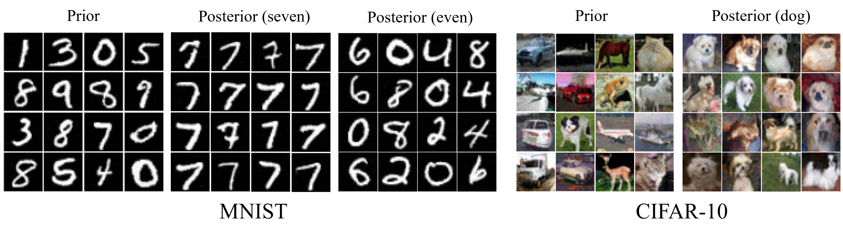
Figure 2: Samples from RTB fine-tuned diffusion posteriors.

4.1 Class-conditional posterior sampling from unconditional diffusion priors

We evaluate RTB in a classifier-guided visual task where we wish to learn a diffusion posterior ${p_{\phi}^{\rm post}({\mathbf{x}}\mid c)\propto p_{\theta}({\mathbf{x}})p(c\mid{\mathbf{x}})}$ given a pretrained diffusion prior $p_{\theta}({\mathbf{x}})$ and a classifier $r({\mathbf{x}})=p(c\mid{\mathbf{x}})$.

Setup.

We consider two 10-class image datasets, MNIST and CIFAR-10, using off-the-shelf unconditional diffusion priors from [26] and standard classifiers $p(c\mid{\mathbf{x}})$ for both datasets. We perform parameter-efficient fine-tuning of $p_{\phi}^{\rm post}$, initialized as a copy of the prior $p_{\theta}$, using the RTB objective (see §E.1 for details). The RTB objective is optimized on trajectories sampled on-policy from the current posterior model. We compare RTB with two RL-based fine-tuning techniques derived from DPOK [15] and DDPO [7] and with two classifier guidance baselines, namely DPS [10], and LGD-MC [68]. We consider three experimental settings: MNIST single-digit posterior (learning to sample images of each digit class $c$), CIFAR-10 single-class posterior (analogous to the previous), and MNIST multi-digit posterior. The latter is a multimodal posterior, for which we set ${r({\mathbf{x}})=\max_{i\in\{0,2,4,6,8\}}p(c=i\mid{\mathbf{x}})}$ to generate even digits, and similarly for odd digits.

Results.

Samples from the RTB-fine-tuned posterior models are shown in Fig. 2. In Table 2 we report mean$\pm\rm std$ of various metrics across all trained posteriors. We observe that models fine-tuned with RTB generate class samples with both the highest diversity (highest mean pairwise cosine distance in Inceptionv3 feature space) and closeness to true samples of the target classes (FID), while achieving high expected $\log r({\mathbf{x}})$. Pure RL fine-tuning (no KL regularization) displays mode collapse characteristics, achieving high rewards in exchange for significantly poorer diversity and FID scores (see also Fig. E.1). Classifier-guidance-based methods, like DP and LGD-MC, exhibit high diversity, but fail to appropriately model the posterior distribution (lowest $\log r({\mathbf{x}})$). Additional results can be found in §E.2.

4.2 Fine-tuning a text-to-image diffusion model

Diffusion models for text-conditional image generation [e.g. 62] can struggle to consistently generate images ${\mathbf{x}}$ that adhere to complex prompts ${\mathbf{z}}$, for example, those that involve composing multiple objects (e.g., “A cat and a dog”) or specify “unnatural” appearances (e.g., “A green-colored rabbit”).Fine-tuning pretrained text-to-image diffusion models $p_{\theta}({\mathbf{x}}_{1}\mid{\mathbf{z}})$ as RL policies to maximize some reward $r({\mathbf{x}}_{1},{\mathbf{z}})$ based on human preferences has become the standard approach to tackle this issue [7, 15, 75]. Simply maximizing the reward function can result in mode collapse as well as over-optimization of the reward. This is typically handled by constraining the fine-tuned model $\tilde{p}$ to be close to the prior $p$:

$$\operatorname*{\arg\!\max}_{\tilde{p}}{\mathbb{E}}_{\tilde{p}({\mathbf{x}}_{1}\mid{\mathbf{z}})}[r({\mathbf{x}}_{1},{\mathbf{z}})],\quad D_{\mathrm{KL}}[\tilde{p}({\mathbf{x}}_{1}\mid{\mathbf{z}})\parallel p({\mathbf{x}}_{1}\mid{\mathbf{z}})]\leq\epsilon.$$ (13)

The optimal $\tilde{p}$ for (13) is $\tilde{p}({\mathbf{x}}_{1}\mid{\mathbf{z}})\propto p({\mathbf{x}}_{1}\mid{\mathbf{z}})\exp(\beta r({\mathbf{x}}_{1},{\mathbf{z}}))$ for some inverse temperature $\beta$. The marginal KL is intractable for diffusion models, so methods like DPOK [15] optimize an upper bound on the marginal KL in the form of a per-step KL penalty $-\gamma\sum_{i=1}^{T}D_{\mathrm{KL}}[\tilde{p}({\mathbf{x}}_{i\Delta t}\mid{\mathbf{x}}_{(i-1)\Delta t},{\mathbf{z}})||p({\mathbf{x}}_{i\Delta t}\mid{\mathbf{x}}_{(i-1)\Delta t},{\mathbf{z}})]$ added to the reward. By contrast, RTB can avoid the bias in such an approximation and directly learn to generate unbiased samples from the posterior $\tilde{p}({\mathbf{x}}_{1}\mid{\mathbf{z}})$.

Setup.

We demonstrate how RTB can be used to fine-tune pretrained text-to-image diffusion models. We use the latent diffusion model Stable Diffusion v1-5 [62] as a prior over $512\times 512$ images. Following DPOK [15], we use ImageReward [85], which has been trained to match human preferences as well as prompt accuracy to attributes such as the number of objects, color, and compositionality, as the reward $\log r({\mathbf{x}}_{1},{\mathbf{z}})$. As reference, we present comparisons against DPOK with the default KL regularization $\gamma=0.01$ and DPOK with $\gamma=0.0$, which is equivalent to DDPO [7].We measure the final average reward and the diversity of the generated image, as measured by the average pairwise cosine distance between CLIP embeddings [57] of a batch of generated images. Further details about the experimental setup and ablations are discussed in §H.

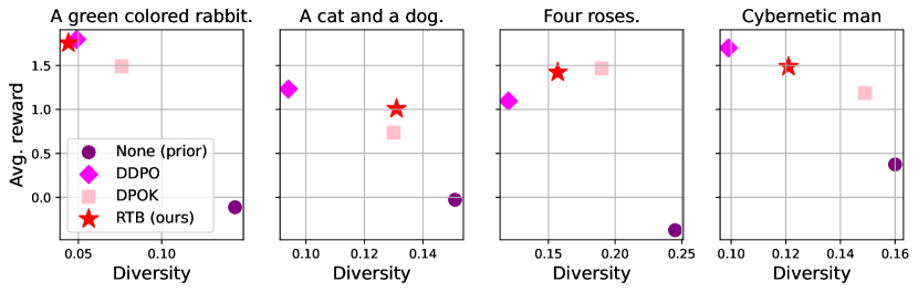
Figure 3: Fine-tuning Stable Diffusion with ImageReward. We report mean $\log r({\mathbf{x}}_{1},{\mathbf{z}})$ and diversity, measured as the mean cosine distance between CLIP embeddings for a batch of 100 generated images.

Results.

footnote 3 plots the diversity versus log reward on a set of prompts from [15, 85]. In terms of average $\log r({\mathbf{x}}_{1},{\mathbf{z}})$, RTB either matches or outperforms DPOK, while generally achieving lower reward than DDPO. The CLIP diversity score for RTB and DPOK are on average higher than DDPO, which is expected since it does not use KL regularization. For qualitative image assessments, refer to Fig. 4 and §H.1. Through this experiment, we show that RTB scales well to high dimensional, multimodal data, matching state-of-the-art methods for fine-tuning text-to-image diffusion models.

(a) Four roses.

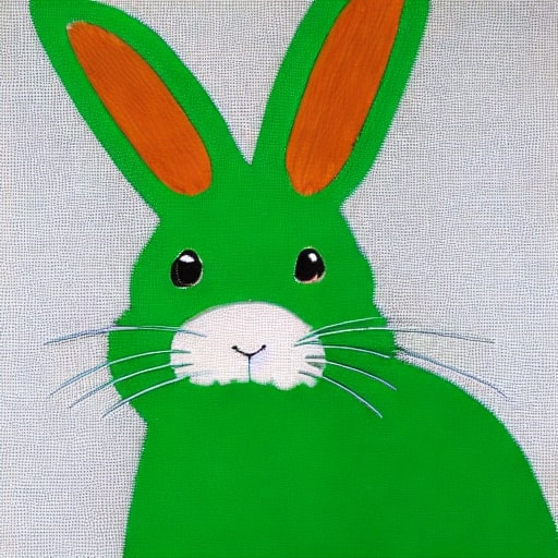
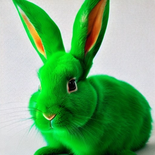
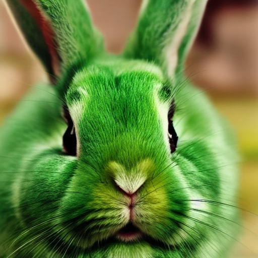
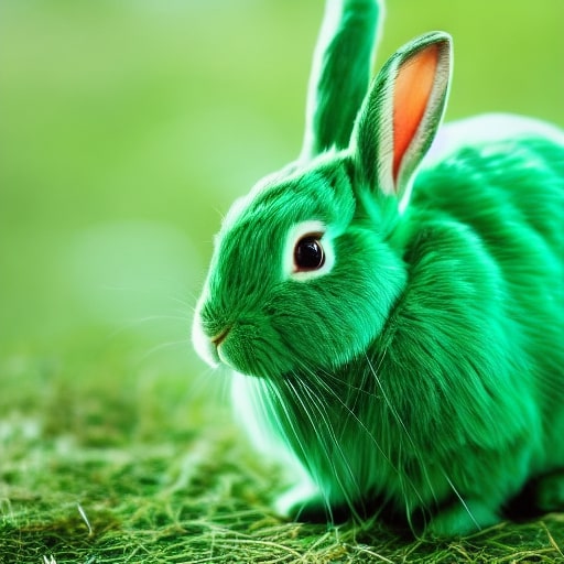
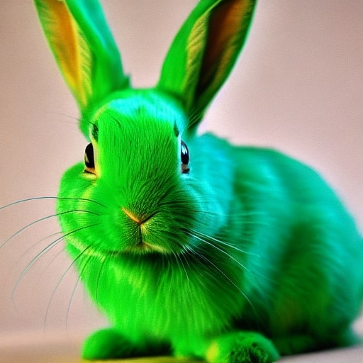
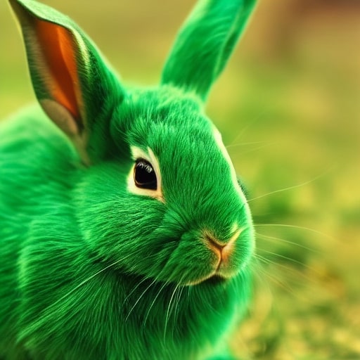
(b) A green rabbit.

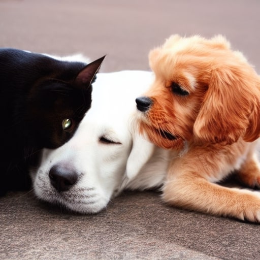
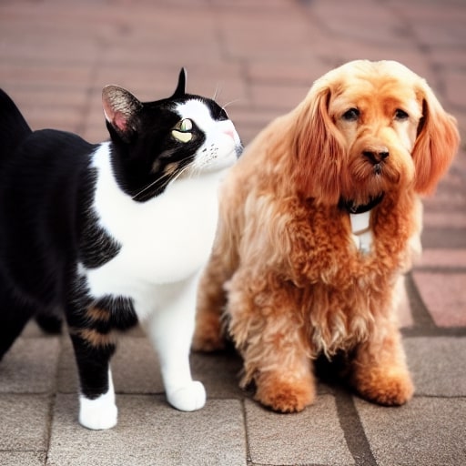
(c) A cat and a dog.

(d) Cybernetic man.

Figure 4: Images generated from prior (top row), DPOK (middle row) and RTB (bottom row) for 4 different prompts. Images in the same column share the random DDIM seed. More images in §H.1.

4.3 Text infilling with discrete diffusion language models

Table 3: Results on the story infilling task with autoregressive and discrete diffusion language models. Metrics are computed with respect to reference infills from the dataset. All metrics are mean$\pm\rm std$ over 5 samples for each of the 100 test examples. RTB with discrete diffusion prior performs better than best baseline with autoregressive prior.

Model	Algorithm $\downarrow$ Metric $\rightarrow$	BLEU-4	GLEU-4	BERTScore
Autoreg.	Prompting	$0.010$$\pm 0.002$	$0.022$$\pm 0.001$	$0.005$$\pm 0.001$
	Supervised fine-tuning	$0.012$$\pm 0.001$	$0.023$$\pm 0.001$	$0.013$$\pm 0.002$
	GFN fine-tuning [28]	blue!10$0.019$$\pm 0.001$	blue!10$0.031$$\pm 0.002$	blue!10$0.102$$\pm 0.005$
Discrete diffusion	Prompt $({\mathbf{x}})$	$0.011$$\pm 0.002$	$0.023$$\pm 0.002$	$0.014$$\pm 0.003$
	Prompt $({\mathbf{x}},{\mathbf{y}})$	$0.014$$\pm 0.003$	$0.027$$\pm 0.003$	$0.092$$\pm 0.004$
	RTB (ours)	blue!10$0.022$$\pm 0.004$	blue!10$0.041$$\pm 0.003$	blue!10$0.122$$\pm 0.004$

To evaluate our approach on discrete diffusion models, we consider the problem of text infilling [89], which involves filling in missing tokens given some context tokens. While discrete diffusion models – unlike their continuous counterparts – can be challenging to train [4, 8, 48, 72], score entropy discrete diffusion [SEDD; 42] matches the language modeling performance of autoregressive language models of similar scale. Non-autoregressive generation in diffusion language models can provide useful inductive biases for infilling, such as the ability to attend to context on both sides of a target token.

Setup.

We use the ROCStories corpus [49], a dataset of short stories containing 5sentences each. We adopt the task setup from [28], where the first 3 sentences of a story ${\mathbf{x}}$ and the last sentence ${\mathbf{y}}$ are given, and the goal is to generate the fourthsentence ${\mathbf{z}}$ such that the overall story is coherent and consistent. The fourth sentence can involve a turning point in the story and is thus challenging to fill in.We aim to model the posterior $p^{\rm post}({\mathbf{z}}\mid{\mathbf{x}},{\mathbf{y}})\propto p({\mathbf{z}}\mid{\mathbf{x}})p_{\text{reward}}({\mathbf{y}}\mid{\mathbf{x}},{\mathbf{z}})$ where $p$ is a SEDD language model prior (a conditional model over ${\mathbf{z}}$ given ${\mathbf{x}}$) and $p_{\text{reward}}$ is an autoregressive language model fine-tuned with a maximum likelihood objective on a held-out subset of the dataset. As baselines, we consider simply prompting the diffusion language model with ${\mathbf{x}}$ and with ${\mathbf{x}},{\mathbf{y}}$. Additionally, to contextualize the performance, we also consider autoregressive language model baselines from [28], which studied this problem under an autoregressive prior $p({\mathbf{z}}\mid{\mathbf{x}})$. See §F for further details about the experimental setup.

Results.

Following [28], we use three standard metrics to measure the similarity of the generated infills with the reference infills from the dataset: BERTScore [88] (with DeBERTa [25]), BLEU-4 [53], and GLEU-4 [84]. Table 3 summarizes the results. We observe that the diffusion language model performs significantly better than the autoregressive language model without any fine-tuning. RTB further improves the performance over prompting, and even outperforms the strongest autoregressive baseline of GFlowNet fine-tuning. We provide some examples of generated text in §F.

4.4 KL-constrained policy search in offline reinforcement learning

The goal of RL algorithms is to learn a policy $\pi(a\mid s)$, i.e., a mapping from states $s$ to actions $a$ in an environment, that maximizes the expected cumulative discounted reward [73]. In the offline RL setting [38],the agent has access to a dataset $\mathcal{D}=\{(s_{t}^{i},a_{t}^{i},s_{t+1}^{i},r_{t}^{i})\}_{i=1}^{N}$ of transitions (where each sample $(s_{t},a_{t},s_{t+1},r_{t})$ indicates that an agent taking action $a_{t}$ at state $s_{t}$ transitioned to the next state $s_{t+1}$ and received reward $r_{t}$). This dataset is assumed to be generated by a behavior policy $\mu(a\mid s)$, which may be a diffusion model trained on ${\mathcal{D}}$. Offline RL algorithms must learn a new policy $\pi$ which achieves high return using only this dataset without interacting with the environment.An important problem in offline RL is policy extraction from trained $Q$-functions [54, 24, 43]. For reliable extrapolation, one wants the policy to predict actions that have high $Q$-values, but also have high density under the behavior policy $\mu$, as naive maximization can result in choosing actions with low probability under $\mu$ and thus unreliable predictions from the $Q$-function. This is formulated as a KL-constrained policy search problem:

$$\operatorname*{\arg\!\max}_{\pi}{\mathbb{E}}_{s\sim d_{\mu},a\sim\pi(a\mid s)}[Q(s,a)],\quad{\mathbb{E}}_{s\sim d_{\mu}}[D_{\mathrm{KL}}(\pi(a\mid s)\parallel\mu(a\mid s))]\leq\epsilon,$$ (14)

where $d_{\mu}$ is the distribution over states induced by following the policy $\mu$. The optimal policy $\pi$ in (14) is the product distribution $\pi^{*}(a\mid s)\propto\mu(a\mid s)\exp(\beta Q(s,a))$ for some inverse temperature $\beta$. If $\mu(a\mid s)$ is a conditional diffusion model over continuous actions $a$ conditioned on state $s$, we use RTB to fine-tune a diffusion behavior policy to sample from $\pi^{*}$, using $\mu$ as the prior and $\exp(\beta Q(s,a))$ as the target constraint. We use a $Q$-function trained using IQL [35].

Setup.

We test on continuous control tasks in the D4RL suite [17], which consists of offline datasets collected using a mixture of SAC policies of varying performance. We evaluate on the halfcheetah, hopper and walker2d MuJoCo [74] locomotion tasks, each of which contains three datasets of transitions: “medium” (collected from an early-stopped policy), “medium-expert” (collected from both an expert and an early-stopped policy) and “medium-replay” (transitions stored in the replay buffer prior to early stopping). We compare against standard offline RL baselines (Behavior Cloning (BC), CQL [36], and IQL [35]) and diffusion-based offline RL methods which are currently state-of-the-art: Diffuser [D; 29], Decision Diffuser [DD; 2], D-QL [81], IDQL [24], and QGPO [43]. For algorithm implementation details, hyperparameters, and a report of baselines, see §G.

Results.

Table 4 shows that RTB matches state-of-the-art results across the D4RL tasks. In particular, RTB performs strongly in the medium-replay tasks, which contain the most suboptimal data and consequently the poorest behavior prior. We highlight that our performance is similar to QGPO [43], which learns intermediate energy densities for diffusion posterior sampling.

Table 4: Average rewards of trained policies on D4RL locomotion tasks (mean$\pm\text{std}$ over 5 random seeds). Following past work, numbers within 5% of maximum in every row are highlighted.

Task $\downarrow$ Algorithm $\rightarrow$	BC	CQL	IQL	D	DD	D-QL	IDQL	QGPO	RTB (ours)
halfcheetah-medium-expert	55.2	blue!1091.6	86.7	79.8	90.6	blue!1096.1	blue!1095.9	blue!1093.5	74.93$\pm 1.72$
hopper-medium-expert	52.5	105.4	91.5	blue!10107.2	blue!10111.8	blue!10110.7	blue!10108.6	blue!10108.0	96.71$\pm 3.53$
walker2d-medium-expert	blue!10107.5	blue!10108.8	blue!10109.6	blue!10108.4	blue!10108.8	blue!10109.7	blue!10112.7	blue!10110.7	blue!10109.52$\pm 0.11$
halfcheetah-medium	42.6	44.0	47.4	44.2	49.1	50.6	51.0	blue!1054.1	blue!1053.70$\pm 0.33$
hopper-medium	52.9	58.5	66.3	58.5	79.3	82.4	65.4	blue!1098.0	82.76$\pm 7.07$
walker2d-medium	75.3	72.5	78.3	79.7	82.5	blue!1085.1	82.5	blue!1086.0	blue!1087.29$\pm 3.15$
halfcheetah-medium-replay	36.6	45.5	44.2	42.2	39.3	blue!1047.5	blue!1045.8	blue!1047.6	blue!1048.11$\pm 0.56$
hopper-medium-replay	18.1	95.0	94.7	blue!1096.8	blue!10100.0	blue!10100.7	92.1	blue!1096.9	blue!10100.40$\pm 0.21$
walker2d-medium-replay	26.0	77.2	73.9	61.2	75.0	blue!1094.3	85.1	84.4	blue!1093.57$\pm 2.63$

5 Other related work

Composing iterative generative processes.

Beyond the approximate posterior sampling algorithms and application-specific techniques discussed in §1 and §4, several recent works have explored the use of hierarchical models, such as diffusion models, as modular components in generative processes. Diffusion models can be used to sample product distributions to induce compositional structure in images [40, 14].Amortized Bayesian inference [34, 59, 58, 19] is another domain of sampling from product distributions where diffusion models are now being used [20].Beyond product models, [18] studies ways to amortize other kinds of compositions of hierarchical processes, including diffusion models, while [65] proposes methods to sample the product of many iterative processes in application to federated learning. Finally, models without hierarchical structure, such as normalizing flows, have been used to amortize intractable inference in pretrained diffusion models [e.g., 16]. In contrast, our method performs posterior inference by fine-tuning a prior model, developing a direction on flexible extraction of information from large pretrained models [28].

Diffusion samplers.

Several prior works seek to amortize MCMC sampling from unnormalized densities by training diffusion models for efficient mode-mixing [6, 87, 76, 61, 77, 3]. Our work is most closely related to continuous GFlowNets [37], which offer an alternative perspective on training diffusion samplers using off-policy flow consistency objectives [37, 86, 64].

6 Conclusions and future work

Relative trajectory balance provides a new approach to training diffusion models to generate unbiased posterior samples given a diffusion prior and an arbitrary reward function. Through experiments on a variety of domains – vision, language, continuous control – we demonstrated the flexibility and general applicability of RTB. RTB can be optimized with off-policy trajectories, and future work can explore ways to leverage off-policy training, using techniques such as local search [33, 64] to improve sample efficiency and mode coverage. Simulation-based objectives in the style of [87] are also applicable to the amortized sampling problems we consider and should be explored, as should simulation-free extensions, e.g., through objectives that are local in time [44]. The ability to handle arbitrary black-box likelihoods also makes RTB a useful candidate for inverse problems in domains such as 3D object synthesis with likelihood computed via a renderer [e.g., 55, 80], imaging problems in astronomy [e.g., 1], medical imaging [e.g., 71], and molecular structure prediction [e.g., 82].

Limitations.

RTB learns the posterior through simulation-based training, which can be slow and memory-intensive. Additionally, the RTB objective is computed on complete trajectories without any local credit-assignment signal, which can result in high variance in the gradients.

Broader impact.

While our contributions focus on an algorithmic approach for learning posterior samplers with diffusion priors, we acknowledge that like other advances in generative modelling, our approach can potentially be used by nefarious actors to train generative models to produce harmful content and misinformation. At the same time, our approach can be also be used to mitigate biases captured in pretrained models and applied to various scientific problems.

Appendix A Proofs

Appendix B Relative TB as TB under the prior measure

The theoretical foundations for continuous generative flow networks [37] establish the correctness of enforcing constraints such as trajectory balance (7) for training sequential samplers, such as diffusion models, to match unnormalized target densities. While we have considered Gaussian transitions and identified transition kernels with their densities with respect to the Lebesgue measure over ${\mathbb{R}}^{d}$, these foundations generalize to more general reference measures. In application to diffusion samplers, suppose that $\pi_{\rm ref}({\mathbf{x}}_{t})$ is a collection of Lebesgue-absolutely continuous densities over ${\mathbb{R}}^{d}$ for $t=0,\Delta t,\dots,1$ and that $\overrightarrow{\pi}_{\rm ref}({\mathbf{x}}_{t}\mid{\mathbf{x}}_{t-\Delta t}),\overleftarrow{\pi}_{\rm ref}({\mathbf{x}}_{t-\Delta t}\mid{\mathbf{x}}_{t})$ are collections of Lebesgue-absolutely continuous transition kernels. If these densities jointly satisfy the detailed balance condition $\pi_{\rm ref}({\mathbf{x}}_{t})\overleftarrow{\pi}_{\rm ref}({\mathbf{x}}_{t-\Delta t}\mid{\mathbf{x}}_{t})=\pi_{\rm ref}({\mathbf{x}}_{t-\Delta t})\overrightarrow{\pi}_{\rm ref}({\mathbf{x}}_{t}\mid{\mathbf{x}}_{t-\Delta t})$, then they satisfy the conditions to be reference measures. A main result of [37] is that if a pair of forward and backward processes satisfies the trajectory balance constraint (7) jointly with a reward density $r$, then the forward process $p$ samples from the distribution with density $r$, with all densities interpreted as relative to the reference measures $\pi_{\rm ref},\overleftarrow{\pi}_{\rm ref},\overrightarrow{\pi}_{\rm ref}$.If $p_{\theta}$ is a diffusion model that satisfies the TB constraint jointly with some reverse process $q$ and target density $q({\mathbf{x}}_{1})$, then one can take the reference transition kernels $\overrightarrow{\pi}_{\rm ref},\overleftarrow{\pi}_{\rm ref}$ to be $p$ and $q$, respectively. In this case, the TB constraint for a target density $\frac{1}{Z}r({\mathbf{x}}_{1})$ and forward transition $p_{\phi}^{\rm post}$ is

$$\frac{p_{\phi}^{\rm post}({\mathbf{x}}_{0},{\mathbf{x}}_{\Delta t},\dots,{\mathbf{x}}_{1})}{\overrightarrow{\pi}_{\rm ref}({\mathbf{x}}_{0},{\mathbf{x}}_{\Delta t},\dots,{\mathbf{x}}_{1})}=\frac{\frac{1}{Z}r({\mathbf{x}}_{1})\cancel{q({\mathbf{x}}_{0},{\mathbf{x}}_{\Delta t},\dots,{\mathbf{x}}_{1-\Delta t}\mid{\mathbf{x}}_{1})}}{\cancel{\overleftarrow{\pi}_{\rm ref}({\mathbf{x}}_{0},{\mathbf{x}}_{\Delta t},\dots,{\mathbf{x}}_{1-\Delta t}\mid{\mathbf{x}}_{1})}},$$ (15)

which is identical to the RTB constraint (8). If (15) holds, then $p_{\phi}^{\rm post}$ samples from the distribution with density $\frac{1}{Z}r({\mathbf{x}}_{1})$ relative to $\pi_{\rm ref}({\mathbf{x}}_{1})$, which is exactly $\frac{1}{Z}p_{\theta}({\mathbf{x}}_{1})r({\mathbf{x}}_{1})$. We have thus recovered RTB as a case of TB for non-Lebesgue reference measures.

Appendix C Posterior inference on two-dimensional Gaussian mixture model

Setup

We conduct toy experiments in low-dimensional spaces using samples from a Gaussian mixture model with multiple modes to visually demonstrate its validity. The prior distribution $p({\mathbf{x}}_{1})$ is trained on a Gaussian mixture model with 25 evenly weighted modes, while the target posterior $p^{\mathrm{post}}({\mathbf{x}}_{1})=r({\mathbf{x}}_{1})p({\mathbf{x}}_{1})$ uses a reward $r({\mathbf{x}}_{1})$ to select and re-weight 9 modes from $p({\mathbf{x}}_{1})$. More specifically, the resulting posterior is:

$$p^{\mathrm{post}}({\mathbf{x}}_{1}) =\frac{1}{\sum_{j}\tilde{\pi}_{j}}\sum_{i}\tilde{\pi}_{i}\mathcal{N}({\mathbf{x}}_{1}\mid\mathbf{\mu}_{i},\mathbf{I})$$ (16)

$$\{\mathbf{\mu}_{i}\} =\{(-10,-5),(-5,-10),(-5,0),(10,-5),(0,0),(0,5),(5,-5),(5,0),(5,10)\}$$ (17)

$$\{\tilde{\pi}_{i}\} =\{4,10,4,5,10,5,4,15,4\}$$ (18)

Our objective is to sample from the posterior $p^{\mathrm{post}}({\mathbf{x}}_{1})$. We compare our method with several baselines, including policy gradient reinforcement learning (RL) with KL constraint and classifier-guided diffusion models. For RL, we implemented the REINFORCE method with a mean baseline and a KL constraint, following recent work training diffusion models to optimize a reward function [7]. Sampling according to the RL policy leads to a distribution $q_{\theta}({\mathbf{x}}_{1})$, which is trained with the objective:

$$J(\theta)=\mathbb{E}_{q_{\theta}({\mathbf{x}}_{1})}\left[r({\mathbf{x}}_{1})\right]+\alpha D_{\mathrm{KL}}\left(q_{\theta}({\mathbf{x}}_{1})\|p({\mathbf{x}}_{1})\right)$$ (19)

While the exact computation of $KL\left(q_{\theta}({\mathbf{x}}_{1})\|p({\mathbf{x}}_{1})\right)$ is intractable, we follow the approximation method introduced by Fan et al. [15], which sums the divergence at every diffusion step. This approximation optimizes an upper bound of the marginal KL.The other baseline is classifier (energy) guidance, which given a diffusion prior, samples using a posterior score function estimate:

$$\nabla_{{\mathbf{x}}_{t}}\log p^{\mathrm{post}}({\mathbf{x}}_{t})\approx\nabla_{{\mathbf{x}}_{t}}\log p({\mathbf{x}}_{t})+\nabla_{{\mathbf{x}}_{t}}\log r({\mathbf{x}}_{t})$$ (20)

Note that this is a biased approximation of the true intractable score:

$$\nabla_{{\mathbf{x}}_{t}}\log p^{\mathrm{post}}({\mathbf{x}}_{t})=\nabla_{{\mathbf{x}}_{t}}\log p({\mathbf{x}}_{t})+\nabla_{{\mathbf{x}}_{t}}\log\mathbb{E}_{p({\mathbf{x}}_{1}\mid{\mathbf{x}}_{t})}[r({\mathbf{x}}_{1})].$$ (21)

For our experiments, we follow the source code provided in recent diffusion sampler benchmarks [64]. We utilize a batch size of 500, with finetuning at 5,000 training iterations, a learning rate of 0.0001, a diffusion time scale of 5.0, 100 steps, and a log variance range of 4.0. The neural architecture employed is identical to that used in [64]. For pretraining the prior model, we use the same hyperparameters as above, but with 10,000 training iterations using maximum likelihood estimation with true samples.

Results.

As we reported in the main text, in Fig. 1, we present illustrative results. The classifier-guided diffusion model shows biased posterior sampling (Fig. 1), failing to provide accurate inference. RL with a per step KL constraint cannot exactly optimize for the posterior distribution, making the tuning of the KL weight $\alpha$ crucial to achieving desirable output Fig. C.1. RTB asymptotically achieves the true posterior without introducing a balancing hyperparameter $\alpha$. Another advantage of our approach is off-policy exploration for efficient mode coverage. RL methods for fine-tuning diffusion models (e.g., DPOK [15], DDPO [7]) typically use policy gradient style methods that are on-policy. By using a simple off-policy trick introduced by [46, 37] and demonstrated by Sendera et al. [64], we can introduce randomness into the exploration process in diffusion by adding $\frac{\epsilon^{2}}{T}$, where $\epsilon$ is a noise hyperparameter and $T$ is the diffusion timestep, into the variances and annealing it to zero over training iterations. We set $\epsilon=0.5$ for off-policy exploration. As shown in Fig. C.2, RTB with off-policy exploration gives very close posterior inferences, whereas off-policy exploration in RL with $\alpha=0.5$ (which is a carefully selected hyperparameter) does not improve performance due to its on-policy nature.

(a) Prior

(b) Posterior

(c) $\alpha=1.0$

(d) $\alpha=0.8$

(e) $\alpha=0.7$

(f) $\alpha=0.5$

(g) $\alpha=0.3$

Figure C.1: Tuning the KL weight $\alpha$ in reinforcement learning: influences the balance between sticking to the prior distribution and moving towards the modes of the reward density. A higher $\alpha$ value maintains closer adherence to the prior, while a lower $\alpha$ allows a gradual shift towards high values of $r({\mathbf{x}})$. Setting $\alpha$ below 0.3 tends to cause mode collapse, moving too far from the prior and focusing on maximizing rewards for single modes. $\alpha=0.5$ gives us samples that closest resembles the posterior.

(a) Prior

(b) Posterior

(c) RTB (on)

(d) RTB (off)

(e) RL (on)

(f) RL (off)

Figure C.2: Off-policy exploration benefits for RTB training. RTB, with simple off-policy exploration techniques that increase randomness in the diffusion process, significantly improves mode coverage. On the other hand, policy gradient RL methods which are typically used to finetune diffusion models are on-policy, and hence prone to mode collapse.

Appendix D Code

Code for all experiments is available at https://github.com/GFNOrg/diffusion-finetuning and willcontinue to be maintained and extended.

Appendix E On classifier guidance and RTB posterior sampling

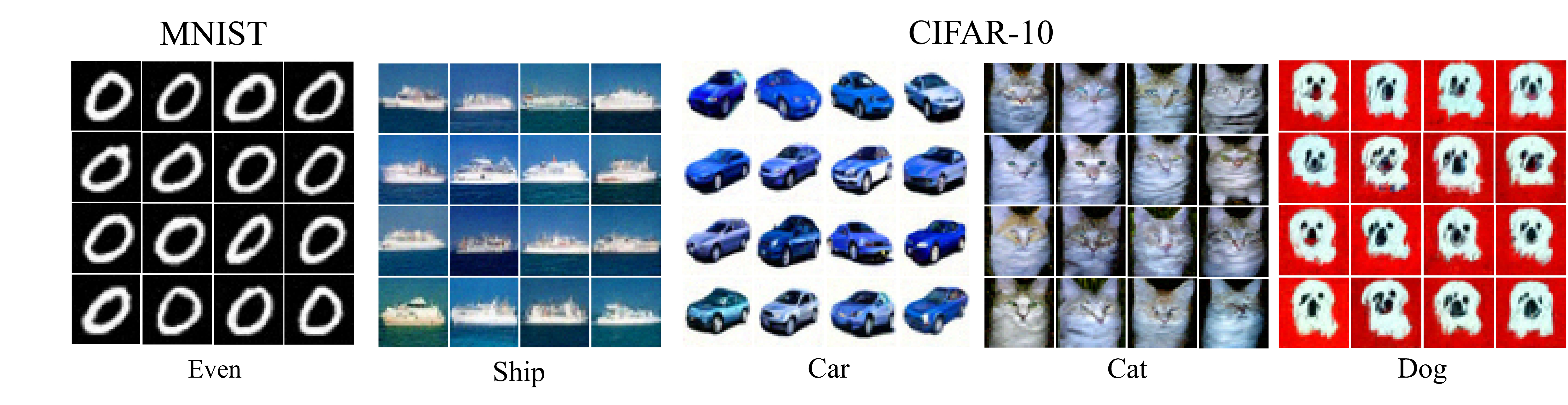
Figure E.1: Samples from a posterior model fine-tuned with RL (no KL). We observe early mode collapse, showcasing high-reward samples with minimal diversity.

E.1 Experimental Details

In our experiments, we fine-tune pretrained unconditional diffusion models with our RTB objective, to sample from a posterior distribution in the form $p^{\rm post}(x\mid y)=p(y\mid x)p(x)$. In this section, we detail the experimental settings for RTB as well as the compared baselines.

Experiments setting.

For MNIST, we pretrain a noise-predicting diffusion model on $28\times 28$ (upscaled to $32\times 32$) single channel images of digits from the MNIST datasets. We discretize the forward and backward processes into 200 steps and train our model until convergence. For CIFAR-10, we use a pretrained model from [26], trained to generate $32\times 32$ 3-channel images from the CIFAR-10 dataset, while discretizing the noising/denoising processes into 1000 steps. For fine-tuning the prior, we parametrize the posterior with LoRA weights [27], with the number of parameters equal to about 3% of the prior model’s parameter count. We train our models on a single NVIDA V100 GPU.We compute FID as a similarity score estimate of the true posterior distribution from the data. As such, the computation is limited to the total number of per-class-samples present in the data, (between 5k and 6k for CIFAR-10 and MNIST digits, and 30k for the even/odd task).

RTB.

For RTB fine-tuning, we finetune a diffusion model following the objective in Equation 10. We impose the objective while sampling denoising paths following a DDPM sampling scheme, with only 20% to 50% of the original trained steps. We employ loss clipping at $0.1$, to account for imperfect constraints in the pretrained prior, and train each of our models for 1500 training iterations, well into convergence trends.

RL  [15].

We implement two RL-based fine-tuning techniques derived from DPOK [15] and DDPO [7], respectively with and without KL regularization. These implementations use a reinforcement learning baseline similar to the one in our experiments described in §4.2. By following the same sampling scheme as in our RTB experiments, we enable a direct comparison with RTB. To fine-tune the KL weight, we perform a search over $\alpha\in\{0.01,0.1,1.0\}$.

DP [10].

We implement and adapt the Gaussian version of the posterior sampling scheme in [10], originally devised for noisy inverse problems. This method relaxes some of our experimental constraints, as it requires a differentiable reward $r({\mathbf{x}})$. We perform a sweep over ten values of the suggest parameter range for the step size $\zeta\in[.1,1.]$ on MNIST single-digit sampling, and choose $\zeta=0.1$ for our experiments.

LGD-MC [68].

We adapt the implementation of the algorithm in [68] to sample from the classifier-based posteriors in CIFAR-10 and MNIST. Similarly to the DP baseline, we use our pretrained classifier to perform measurements at each sampling step, and use a Monte Carlo estimate of the gradient correction to guide the denoising process. We choose $\zeta=0.1$ following the DP experiments and default the number of particles to 10 as per the authors’ guidelines.

E.2 Additional findings.

Classifier-guidance baselines.

We find that the DP and LGD-MC classifier-guidance based baselines struggle to sample from the true posterior distribution in our experimental settings. The baselines achieve the lowers classifier average rewards in all tested settings. Despite choosing $\zeta=0.1$ as the validate best performing hyperparameter, we also also observe the posterior samples from DP and LGD-MC to be close to the prior. As such, DP and LGD-MC score high in diversity, and low in FID for the Even/Odd experimental scenario, as expected from prior sampling benchmarks, but failing to appropriately model the posterior distribution.

RL and mode collapse.

In the pure Reinforcement Learning objective imposed for the experiments in §4.1 (no KL), we observe a significantly higher reward than other baseline methods, while showcasing increased FID and lower diversity. In Fig. E.1 we show a random set of 16 samples for posterior models trained on 4 different classes of the CIFAR-10 datasets, as well as the Even objective from the MNIST dataset, after 500 training iterations. In the figure, we observe early mode collapse and reward exploitation, visually evident from the little to no variation amongst samples for each class class, and single-digit collapse in the multi-modal even digits objective (see samples in Fig. 2 for comparison with our RTB-finetuned models).

Appendix F Infilling with discrete diffusion

Additional details.

We illustrate some examples from the ROC Stories dataset used for training in Table F.1. For the prior we use the sedd-small model, which uses an absorbing noising process [4] with a log linear noise schedule, as the diffusion prior $p({\mathbf{z}}\mid{\mathbf{x}})$. The posterior model is parameterized as a copy of the prior. To condition the diffusion model on the beginning ${\mathbf{x}}$ we set the tokens at the appropriate location in the state in the initial time step, i.e.$t=0$. Our implementation is based on the original SEDD codebase . Training this model is computationally expensive (in terms of memory and speed) so we utilize the stochastic TB trick, only propagating the gradients through a subset of the steps of the trajectory. We also use the loss clipping trick as discussed in §3.2. Specifically, we clip the loss below a certain threshold to 0, resulting in updates only when the loss is larger. This threshold -- referred to as the loss clipping coefficient -- is a hyperparameter. As this is a conditional problem we also use the relative VarGrad objective. We also use some tempering on the reward likelihood which helps in learning (i.e., $p_{\text{reward}}({\mathbf{y}}\mid{\mathbf{x}},{\mathbf{z}})^{\beta}$) where $\beta$ is the inverse temperature parameter. We perform all experiments on an NVIDIA A100-Large GPU.Note that we also tried a baseline of simply fine-tuning the diffusion model on the data but encountered some training instabilities that we could not fix.The hyperparameters used for training RTB in our experiments are detailed in Table F.2.

Reward.

For training $p_{\text{reward}}$ we follow the training procedure and implementation from [28]. Specifically, we fine-tune a GPT-2 Large model [56] on the stories dataset with full parameter fine-tuning using the trl library [79].We trained for 20 epochs with a batch size of 64 and 32 gradient accumulation steps and a learning rate of 0.0005.

Baselines.

For the baselines, we adopt the implementations from [28]. A critical difference in our experiments compared to [28] is that the posterior model is not initialized with a base model that is fine-tuned on the stories dataset. To condition the model on $X$ and $Y$, as well as for the prompting baseline, we use the following prompt:"Beginning: {X}\n End: {Y}\n Middle: "During training for the autoregressive GFlowNet fine-tuning, a $({\mathbf{x}},{\mathbf{y}})$ pair is sampled from the dataset and then sample (batch size) ${\mathbf{x}}$s for every $(X,Y)$, and $p_{\rm reward}(XZY)$ is used as the reward. Both the GFlowNet fine-tuning and supervised fine-tuning baseline use LoRA fine-tuning. We use the default hyperparamteres from [28].At test time, we sample $100$ infills for each example in the test set from all the models at temperature $0.9$, and average over 5 such draws.

Table F.1: Examples of training samples for the language infilling task.

Beginning (${\mathbf{x}}$)	Middle (${\mathbf{z}}$)	End (${\mathbf{y}}$)
I was going to a Halloween party. I looked through my clothes but could not find a costume. I cut up my old clothes and constructed a costume.	I put my costume on and went to the party.	My friends loved my costume.
Allen thought he was a very talented poet. He attended college to study creative writing. In college, he met a boy named Carl.	Carl told him that he wasn’t very good.	Because of this, Allen swore off poetry forever.

Table F.2: Hyperparameters for the story infilling task.

Batch size	16
Gradient accumulation steps	8
Learning rate	1e-5
Warmup Step	20
Optimizer	AdamW
Reward temperature start	1.2
Reward inverse temperature end	0.9
Reward inverse temperature horizon	5000
Number of training steps	1500
Loss clipping coefficient	0.1
Discretization steps $T$	15

Additional Results.

Table F.3, Table F.4 and Table F.5 illustrates some examples of the infills generated by the diffusion models. We note that the general quality of the samples is poor, due to a relatively weak prior. At the same time we can observe that the prompting baselines often generate infills that are unrelated to the current story. We also note that the RTB fine-tuned model can sometimes generate repitions as the reward model tends to assign high likelihood to repititions [83].We also attempted a LLMEval [41] for evaluating the coherence of the stories but did not obtain statistically significant results.

Table F.3: Examples of infills generated by the posterior trained with RTB along with reference infills for the stories infilling task.

Beginning (${\mathbf{x}}$)	Middle (${\mathbf{z}}$)	End (${\mathbf{y}}$)
David noticed he had put on a lot of weight recently. He examined his habits to try and figure out the reason. He realized he’d been eating too much fast food lately.	He stopped going to burger places and started a vegetarian diet.	After a few weeks, he started to feel much better.
	He reviewed his habits to try to figure out how to change
	He asked he thought try to cut down on the amount amount.
	He examined his habits to try and figure out the reason.
	He realized he had been eating too much fast food recently.
Robbie was competing in a cross country meet. He was halfway through when his leg cramped up. Robbie wasn’t sure he could go on.	He stopped for a minute and stretched his bad leg.	Robbie began to run again and finished the race in second place.
	Robbie was sure he could go on. Robbie was sure.
	He was floating and twisting his leg in half then.
	His body just caught up with his legs. Robbie was.
	He held his leg forward as he went through and his

Table F.4: Examples of infills generated by Prompt $({\mathbf{x}},{\mathbf{y}})$ along with reference infills for the stories infilling task.

Beginning (${\mathbf{x}}$)	Middle (${\mathbf{z}}$)	End (${\mathbf{y}}$)
David noticed he had put on a lot of weight recently. He examined his habits to try and figure out the reason. He realized he’d been eating too much fast food lately.	He stopped going to burger places and started a vegetarian diet.	After a few weeks, he started to feel much better.
	He’d had less opportunities to eat properly all of last.
	Doctors made the note of the situation. He was treated.
	He told him the guy for a mic replacement.\n\n
	He felt empty for one reason and new fresh, too.
Robbie was competing in a cross country meet. He was halfway through when his leg cramped up. Robbie wasn’t sure he could go on.	He stopped for a minute and stretched his bad leg.	Robbie began to run again and finished the race in second place.
	Robbie wasn’t sure Robbie’s fuel tank was full.
	Robbie took a photograph with a close friend.\n\n
	Only Stacey Ebers and Rand were out there.
	Robbie got bigger as the position got better.\n\n

Table F.5: Examples of infills generated by Prompt $({\mathbf{x}})$ along with reference infills for the stories infilling task.

Beginning (${\mathbf{x}}$)	Middle (${\mathbf{z}}$)	End (${\mathbf{y}}$)
David noticed he had put on a lot of weight recently. He examined his habits to try and figure out the reason. He realized he’d been eating too much fast food lately.	He stopped going to burger places and started a vegetarian diet.	After a few weeks, he started to feel much better.
	David, "All I had told eat was a problem.
	He got the backside what about that and he made the,
	He made just good of fast food and spliced it down.
	He explained everything to them, reached them out, the problem.
Robbie was competing in a cross country meet. He was halfway through when his leg cramped up. Robbie wasn’t sure he could go on.	He stopped for a minute and stretched his bad leg.	Robbie began to run again and finished the race in second place.
	Robbie and Robbie was piling. Robbie and Robbie fistfight.
	I said goodbye. Robbie at dinner. Robbie agreed with.
	He cut away a little to Robbie’s pace fleetingly.
	He held off all the police and place. Robbie.

Appendix G Offline RL

G.1 Training details

Our method requires first training a diffusion-based behavior policy $\pi_{\theta}$ and a Q-function $Q_{\psi}$. Once $\pi_{\theta}$ and $Q_{\psi}$ are trained, The posterior policy $\pi_{\gamma}$ is trained using RTB, with its weights initialized to the trained behavior policy weights $\theta$.The behavior policy $\pi_{\theta}$ is parametrized as a state-conditioned noise-predicting denoising diffusion probabilistic model (DDPM) [26] with a linear schedule, and 75 denoising steps. The diffusion model takes as input a state $s$, a noised action $a_{t}$ and a noise level $t$ and predicts the source noise $\epsilon$. The state $s$ and noised action $a_{t}$ are concatenated with Fourier features computed on the noise level $t$, which are then fed through a 3-layer MLP of hidden dimensionality 256, with layer normalization and a GeLU activation after each hidden layer. The behavior policy is trained using the Adam optimizer with batch size 512 and learning rate 5e-4 for 10000 epochs. The Q-function $Q_{\psi}$ is trained using IQL. We use the same IQL experimental configurations and training hyperparameters as in [35]. That is, we set $\tau=0.7$. The architecture for $Q_{\psi}$ is a 3-layer MLP with hidden dimensionality 256 and ReLU activations, which is trained using the Adam optimizer with a learning rate 3e-4 and batch size 256 for 750000 gradient steps. The task rewards are normalized as in [35] and the target network is updated with soft updates of $m=0.005$. The posterior policy $\pi_{\gamma}$ is trained using the relative trajectory balance objective. $\pi_{\gamma}$ is also parametrized as a state-conditioned noise-predicting DDPM, initialized as a copy of the prior. We additionally use the Langevin dynamics inductive bias (12), and learn an additional MLP for the energy scaling network. The posterior noise prediction network also outputs an additive correction to the output of the prior noise prediction network. That is, the predicted noise of the posterior diffusion model is defined as $\epsilon(s,a_{t},t):=\epsilon(s,a_{t},t;\theta)+\epsilon(s,a_{t},t;\gamma)$, where $\epsilon(\cdot;\theta)$ is the output of the prior noise prediction network and $\epsilon(\cdot;\gamma)$ is the output of the posterior noise prediction network. We train all models on a single NVIDIA A100-Large GPU. The only hyperparameter tuned per task is the temperature $\alpha$ which we show in Table G.2.Note that in these experiments both the prior and constraint are conditioned on the state ${\mathbf{s}}$. To prevent having to learn a neural network for $\log Z_{\phi}({\mathbf{s}})$, we employ a variant of VarGrad objective [60]. For each state ${\mathbf{s}}$ sampled in the minibatch, we further generate $k=64$ on-policy trajectories ${\tau^{(i)}}_{i=1}^{k}$ with $\pi_{\gamma}$. Each of these trajectories can be used to implicitly estimate $\log Z({\mathbf{s}})$:

$$\hat{\log Z({\mathbf{s}})}^{(i)}=\log\pi_{\theta}(\tau^{(i)}\mid{\mathbf{s}})+Q_{\psi}({\mathbf{s}},{\mathbf{a}}_{1}^{(i)})-\log\pi_{\gamma}(\tau^{(i)}\mid{\mathbf{s}})$$ (22)

We then minimize the sample variance across the batch:

$${\mathcal{L}}_{\rm RTB}^{\rm VarGrad}(\gamma)=\frac{1}{k}\sum_{i=1}^{k}\Bigl{(}\hat{\log Z({\mathbf{s}})}^{(i)}-\frac{1}{k}\sum_{j=1}^{k}\hat{\log Z({\mathbf{s}})}^{(j)}\Bigr{)}^{2}$$ (23)

Table G.1: Mixed vs. online training on DR4L Tasks. We report mean$\pm\text{std}$ over 5 random seeds.

Task	RTB (Online)	RTB (Mixed)
halfcheetah-medium-replay	46.88$\pm 0.51$	blue!1048.11$\pm 0.56$
hopper-medium-replay	99.23$\pm 3.22$	blue!10100.40$\pm 0.21$
walker2d-medium-replay	blue!1094.01$\pm 0.28$	93.57$\pm 2.63$

RTB allows off-policy training so we are not restricted to train with samples generated on-policy. We thus also leverage the offline dataset, which are samples from the prior and noise them with the DDPM noising process to generate off-policy trajectories with high density under the prior. Since there are actions in the replay buffer from high reward episodes in the tasks, this can help training efficiency compared to purely online training. We ran 5 seeds of training each with mixed training (off-policy and on-policy) and pure on-policy training on the medium-replay tasks, with results shown in Table G.1, where mixed training outperforms pure online training on two of the three tasks.

Table G.2: Temperature $\alpha=\frac{1}{\beta}$ for D4RL tasks

Task	$\alpha$
halfcheetah-medium-expert	0.1
hopper-medium-expert	0.5
walker2d-medium-expert	0.1
halfcheetah-medium	0.05
hopper-medium	0.1
walker2d-medium	0.05
halfcheetah-medium-replay	0.05
hopper-medium-replay	0.05
walker2d-medium-replay	0.1

G.2 Baseline details

As is standard in offline RL, we use the reported performance numbers from the previous papers. CQL, IQL are reported from the IQL paper. Diffuser (D), DD, D-QL and QGPO are reported from the QGPO paper. Their implementation improved the performance of D and D-QL compared to their original papers. IDQL results are reported from the IDQL paper. We follow the evaluation protocol of previous work, and report the mean performance over 10 episodes, averaged across 5 random seeds at the end of training (150k training steps).

Appendix H Fine-tuning text-to-image diffusion models

We build off the DPOK implementation, which fine-tunes stable-diffusion-v1-5 with ImageReward function. The posterior model to be fine-tuned is initialized as a copy of the prior model. We use LoRA [27] since it is significantly more efficient than fine-tuning the entire model. Sampling of images is done with 50 steps of DDIM [67]. Even with LoRA, it is still difficult to fit gradients of all steps in the diffusion trajectory in memory. To help with this, we use a ‘‘stochastic subsampling’’ trick where gradients are only computed for a randomly sampled subset of timesteps in the trajectory. This trick does not change the expected gradient (apart from a scaling factor) while significantly saving memory consumption. It does increase gradient variance, so it is preferable to keep gradients for as many timesteps as possible to fit in memory. For our text-to-image experiments, we found sampling 8 timesteps out of 50 to keep gradients was sufficient. We train all models on a single NVIDIA A100-Large GPU. For the main experiments, we use the default parameters for DPOK of reward weight $\beta=10$ and KL weight $=0.01$. For RTB we fix $\beta=1.0$ for all prompts. We next perform an ablation over different values of $\beta$.We plot in LABEL:tab:betaablation the final average reward and diversity score for models trained with different values of reward weight $\beta$ for the prompt ‘‘A green colored rabbit.’’. As expected, we find that increasing $\beta$ increases reward at the cost of diversity for RTB and DPOK. The exception is $\beta=10$ for RTB which has slightly lower final reward than $\beta=1$, which we could attribute to more difficult optimization due to the peaky distribution associated with higher reward weight.

Table H.1: Ablation of reward weights $\beta$ for ‘‘A green colored rabbit.’’.

Model $\downarrow$	$\beta$ $\downarrow$ Metric $\rightarrow$	Reward ($\uparrow$)	diversity ($\uparrow$)
Prior	-	-0.113	0.597
DPOK (KL weight=0.01)	$\beta=0.01$	-0.27	0.1488
	$\beta=0.1$	-0.06	0.1486
	$\beta=1.0$	0.638	0.1362
	$\beta=10.0$	1.492	0.076
DDPO (KL weight=0.0)	$\beta=10.0$	1.795	0.0493
RTB	$\beta=0.01$	0.485	0.1431
	$\beta=0.1$	1.525	0.0721
	$\beta=1.0$	1.756	0.0436
	$\beta=10.0$	1.568	0.0689

H.1 Generated Images

H.1.1 A green-colored rabbit

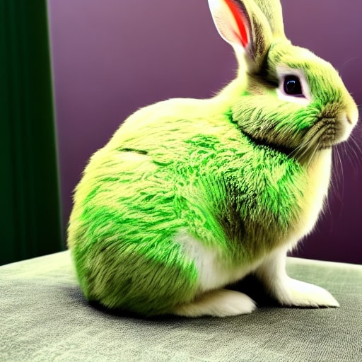
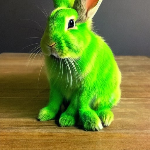
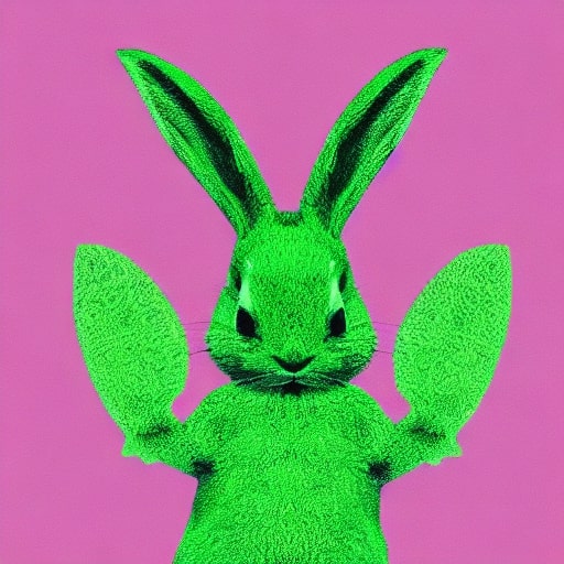
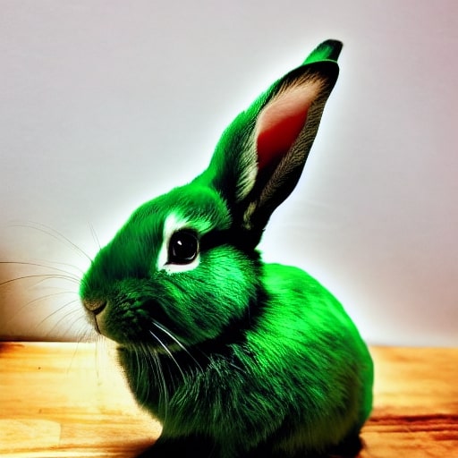
Figure H.1: Prior

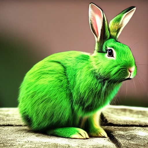
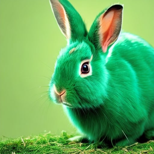
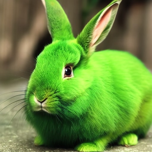
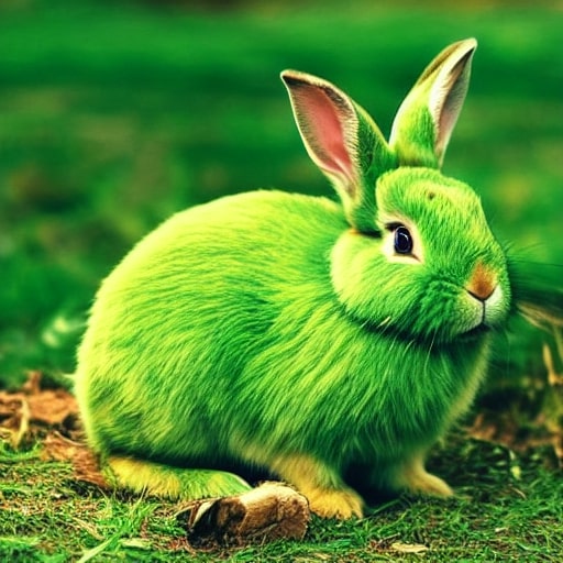
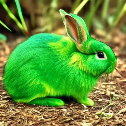
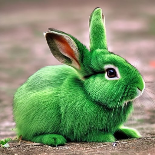
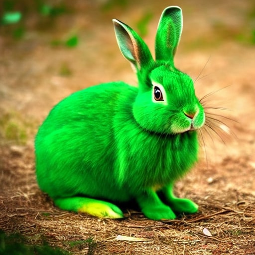
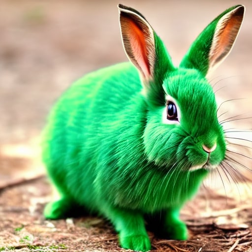
Figure H.2: DDPO

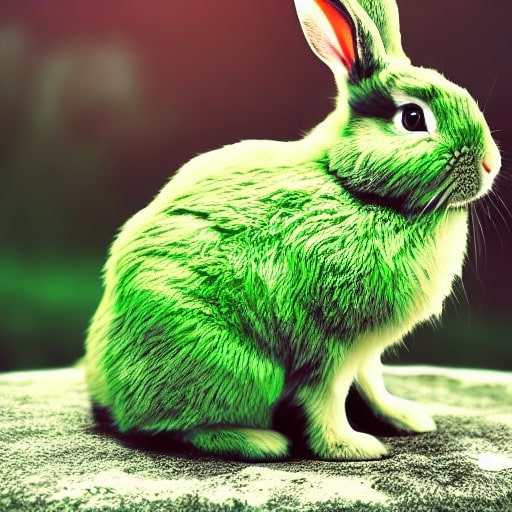
Figure H.3: DPOK

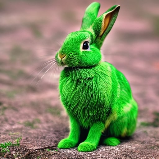
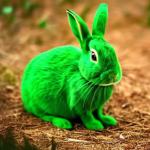
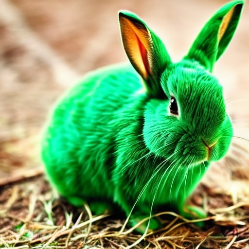
Figure H.4: RTB

H.1.2 Four roses

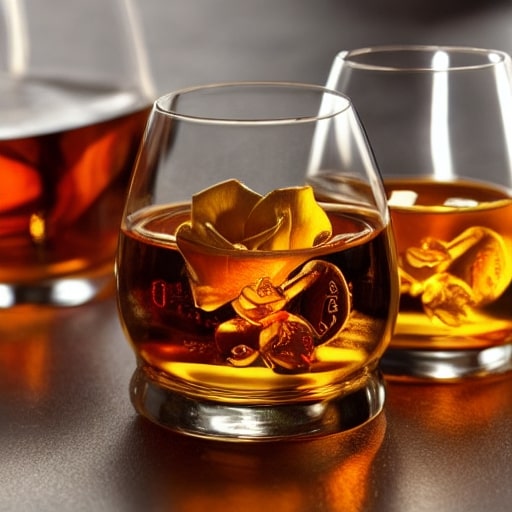
Figure H.5: Prior

Figure H.6: DDPO

Figure H.7: DPOK

Figure H.8: RTB

H.1.3 A cat and a dog

Figure H.9: Prior

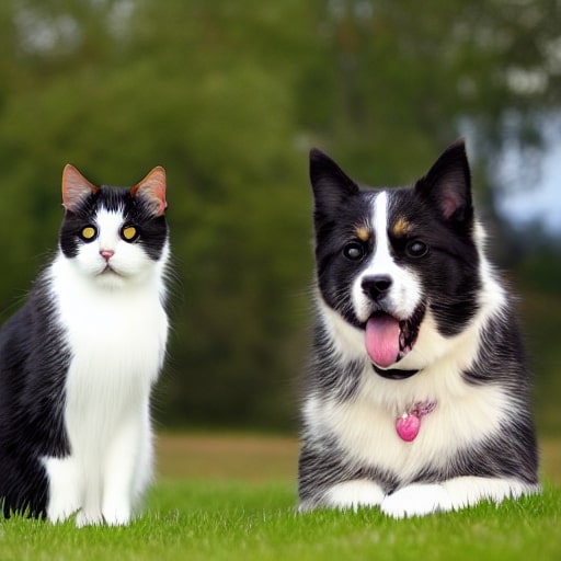
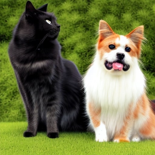
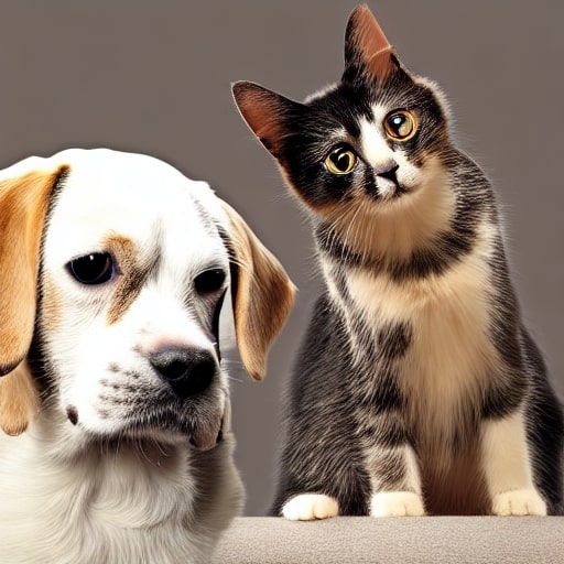
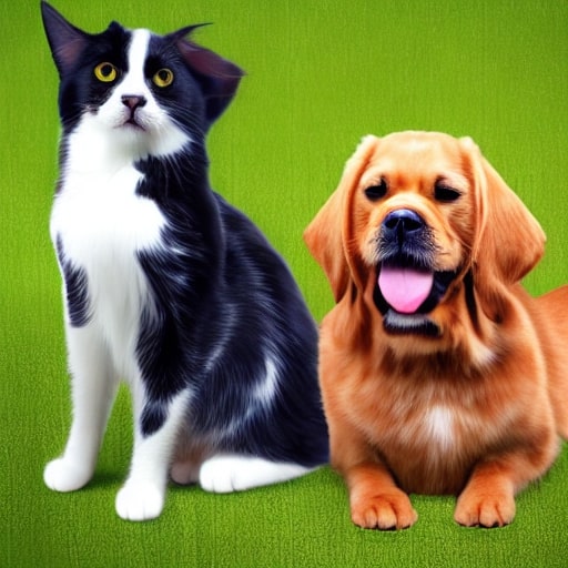
Figure H.10: DDPO

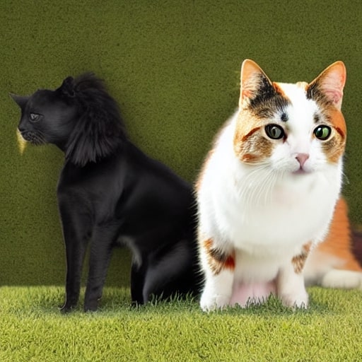
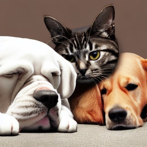
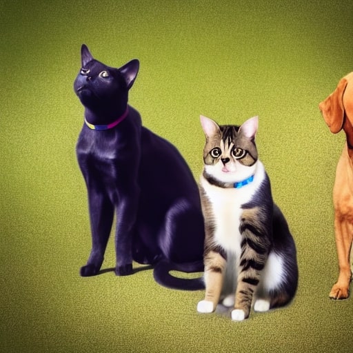
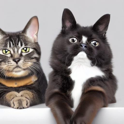
Figure H.11: DPOK

Figure H.12: RTB

H.1.4 A half - masked rugged laboratory engineer man with cybernetic enhancements as seen from a distance, scifi character portrait by greg rutkowski, esuthio, craig mullins.

Figure H.13: Prior

Figure H.14: DDPO

Figure H.15: DPOK

Figure H.16: RTB

Appendix I Compute resources

For classifier guidance experiments §4.1 we use train on a single NVIDIA V100 GPU. For text-conditional image generation §4.2, text infilling §F and offline §G, we use a single NVIDIA A100 large GPU. The total estimated compute time for all our experiments is 3000 hours.

References

- Adam et al. [2022] Alexandre Adam, Adam Coogan, Nikolay Malkin, Ronan Legin, Laurence Perreault-Levasseur, Yashar Hezaveh, and Yoshua Bengio. Posterior samples of source galaxies in strong gravitational lenses with score-based priors. arXiv preprint arXiv:2211.03812, 2022.
- Ajay et al. [2023] Anurag Ajay, Yilun Du, Abhi Gupta, Joshua B. Tenenbaum, Tommi S. Jaakkola, and Pulkit Agrawal. Is conditional generative modeling all you need for decision making? International Conference on Learning Representations (ICLR), 2023.
- Akhound-Sadegh et al. [2024] Tara Akhound-Sadegh, Jarrid Rector-Brooks, Avishek Joey Bose, Sarthak Mittal, Pablo Lemos, Cheng-Hao Liu, Marcin Sendera, Siamak Ravanbakhsh, Gauthier Gidel, Yoshua Bengio, Nikolay Malkin, and Alexander Tong. Iterated denoising energy matching for sampling from Boltzmann densities. International Conference on Machine Learning (ICML), 2024.
- Austin et al. [2021] Jacob Austin, Daniel D Johnson, Jonathan Ho, Daniel Tarlow, and Rianne Van Den Berg. Structured denoising diffusion models in discrete state-spaces. Neural Information Processing Systems (NeurIPS), 2021.
- Bengio et al. [2023] Yoshua Bengio, Salem Lahlou, Tristan Deleu, Edward J. Hu, Mo Tiwari, and Emmanuel Bengio. GFlowNet foundations. Journal of Machine Learning Research, 24(210):1–55, 2023.
- Berner et al. [2024] Julius Berner, Lorenz Richter, and Karen Ullrich. An optimal control perspective on diffusion-based generative modeling. Transactions on Machine Learning Research (TMLR), 2024.
- Black et al. [2024] Kevin Black, Michael Janner, Yilun Du, Ilya Kostrikov, and Sergey Levine. Training diffusion models with reinforcement learning. International Conference on Learning Representations (ICLR), 2024.
- Campbell et al. [2022] Andrew Campbell, Joe Benton, Valentin De Bortoli, Thomas Rainforth, George Deligiannidis, and Arnaud Doucet. A continuous time framework for discrete denoising models. Neural Information Processing Systems (NeurIPS), 2022.
- Cardoso et al. [2024] Gabriel Cardoso, Yazid Janati el idrissi, Sylvain Le Corff, and Eric Moulines. Monte carlo guided denoising diffusion models for bayesian linear inverse problems. International Conference on Learning Representations (ICLR), 2024.
- Chung et al. [2023] Hyungjin Chung, Jeongsol Kim, Michael Thompson Mccann, Marc Louis Klasky, and Jong Chul Ye. Diffusion posterior sampling for general noisy inverse problems. International Conference on Learning Representations (ICLR), 2023.
- Dhariwal and Nichol [2021] Prafulla Dhariwal and Alexander Nichol. Diffusion models beat GANs on image synthesis. Neural Information Processing Systems (NeurIPS), 2021.
- Dieleman et al. [2022] Sander Dieleman, Laurent Sartran, Arman Roshannai, Nikolay Savinov, Yaroslav Ganin, Pierre H Richemond, Arnaud Doucet, Robin Strudel, Chris Dyer, Conor Durkan, et al. Continuous diffusion for categorical data. arXiv preprint arXiv:2211.15089, 2022.
- Dou and Song [2024] Zehao Dou and Yang Song. Diffusion posterior sampling for linear inverse problem solving: A filtering perspective. International Conference on Learning Representations (ICLR), 2024.
- Du et al. [2023] Yilun Du, Conor Durkan, Robin Strudel, Joshua B. Tenenbaum, Sander Dieleman, Rob Fergus, Jascha Sohl-Dickstein, Arnaud Doucet, and Will Sussman Grathwohl. Reduce, reuse, recycle: Compositional generation with energy-based diffusion models and MCMC. International Conference on Machine Learning (ICML), 2023.
- Fan et al. [2023] Ying Fan, Olivia Watkins, Yuqing Du, Hao Liu, Moonkyung Ryu, Craig Boutilier, Pieter Abbeel, Mohammad Ghavamzadeh, Kangwook Lee, and Kimin Lee. Reinforcement learning for fine-tuning text-to-image diffusion models. Neural Information Processing Systems (NeurIPS), 2023.
- Feng et al. [2023] Berthy T. Feng, Jamie Smith, Michael Rubinstein, Huiwen Chang, Katherine L. Bouman, and William T. Freeman. Score-based diffusion models as principled priors for inverse imaging. International Conference on Computer Vision (ICCV), 2023.
- Fu et al. [2020] Justin Fu, Aviral Kumar, Ofir Nachum, George Tucker, and Sergey Levine. D4RL: Datasets for deep data-driven reinforcement learning. arXiv preprint arXiv:2004.07219, 2020.
- Garipov et al. [2023] Timur Garipov, Sebastiaan De Peuter, Ge Yang, Vikas Garg, Samuel Kaski, and Tommi Jaakkola. Compositional sculpting of iterative generative processes. Neural Information Processing Systems (NeurIPS), 2023.
- Garnelo et al. [2018] Marta Garnelo, Jonathan Schwarz, Dan Rosenbaum, Fabio Viola, Danilo J Rezende, SM Eslami, and Yee Whye Teh. Neural processes. arXiv preprint arXiv:1807.01622, 2018.
- Geffner et al. [2023] Tomas Geffner, George Papamakarios, and Andriy Mnih. Compositional score modeling for simulation-based inference. International Conference on Machine Learning (ICML), 2023.
- Graikos et al. [2022] Alexandros Graikos, Nikolay Malkin, Nebojsa Jojic, and Dimitris Samaras. Diffusion models as plug-and-play priors. Neural Information Processing Systems (NeurIPS), 2022.
- Gulrajani and Hashimoto [2023] Ishaan Gulrajani and Tatsunori B Hashimoto. Likelihood-based diffusion language models. Neural Information Processing Systems (NeurIPS), 2023.
- Han et al. [2023] Xiaochuang Han, Sachin Kumar, and Yulia Tsvetkov. SSD-LM: Semi-autoregressive simplex-based diffusion language model for text generation and modular control. Association for Computational Linguistics (ACL), 2023.
- Hansen-Estruch et al. [2023] Philippe Hansen-Estruch, Ilya Kostrikov, Michael Janner, Jakub Grudzien Kuba, and Sergey Levine. IDQL: Implicit Q-learning as an actor-critic method with diffusion policies. arXiv preprint arXiv:2304.10573, 2023.
- He et al. [2021] Pengcheng He, Xiaodong Liu, Jianfeng Gao, and Weizhu Chen. Deberta: Decoding-enhanced bert with disentangled attention. International Conference on Learning Representations (ICLR), 2021.
- Ho et al. [2020] Jonathan Ho, Ajay Jain, and Pieter Abbeel. Denoising diffusion probabilistic models. Neural Information Processing Systems (NeurIPS), 2020.
- Hu et al. [2022] Edward J. Hu, yelong shen, Phillip Wallis, Zeyuan Allen-Zhu, Yuanzhi Li, Shean Wang, Lu Wang, and Weizhu Chen. LoRA: Low-rank adaptation of large language models. International Conference on Learning Representations (ICLR), 2022.
- Hu et al. [2024] Edward J. Hu, Moksh Jain, Eric Elmoznino, Younesse Kaddar, Guillaume Lajoie, Yoshua Bengio, and Nikolay Malkin. Amortizing intractable inference in large language models. International Conference on Learning Representations (ICLR), 2024.
- Janner et al. [2022] Michael Janner, Yilun Du, Joshua Tenenbaum, and Sergey Levine. Planning with diffusion for flexible behavior synthesis. International Conference on Machine Learning (ICML), 2022.
- Kadkhodaie and Simoncelli [2021] Zahra Kadkhodaie and Eero P. Simoncelli. Solving linear inverse problems using the prior implicit in a denoiser. Neural Information Processing Systems (NeurIPS), 2021.
- Kang et al. [2024] Bingyi Kang, Xiao Ma, Chao Du, Tianyu Pang, and Shuicheng Yan. Efficient diffusion policies for offline reinforcement learning. Neural Information Processing Systems (NeurIPS), 2024.
- Kawar et al. [2021] Bahjat Kawar, Gregory Vaksman, and Michael Elad. SNIPS: Solving noisy inverse problems stochastically. Neural Information Processing Systems (NeurIPS), 2021.
- Kim et al. [2024] Minsu Kim, Taeyoung Yun, Emmanuel Bengio, Dinghuai Zhang, Yoshua Bengio, Sungsoo Ahn, and Jinkyoo Park. Local search GFlowNets. International Conference on Learning Representations (ICLR), 2024.
- Kingma and Welling [2014] Diederik P. Kingma and Max Welling. Auto-encoding variational Bayes. International Conference on Learning Representations (ICLR), 2014.
- Kostrikov et al. [2022] Ilya Kostrikov, Ashvin Nair, and Sergey Levine. Offline reinforcement learning with implicit Q-learning. International Conference on Learning Representations (ICLR), 2022.
- Kumar et al. [2020] Aviral Kumar, Aurick Zhou, George Tucker, and Sergey Levine. Conservative Q-learning for offline reinforcement learning. Neural Information Processing Systems (NeurIPS), 2020.
- Lahlou et al. [2023] Salem Lahlou, Tristan Deleu, Pablo Lemos, Dinghuai Zhang, Alexandra Volokhova, Alex Hernández-Garcıa, Léna Néhale Ezzine, Yoshua Bengio, and Nikolay Malkin. A theory of continuous generative flow networks. International Conference on Machine Learning (ICML), 2023.
- Levine et al. [2020] Sergey Levine, Aviral Kumar, G. Tucker, and Justin Fu. Offline reinforcement learning: Tutorial, review, and perspectives on open problems. arXiv preprint arXiv:2005.01643, 2020.
- Li et al. [2022] Xiang Li, John Thickstun, Ishaan Gulrajani, Percy S Liang, and Tatsunori B Hashimoto. Diffusion-LM improves controllable text generation. Neural Information Processing Systems (NeurIPS), 2022.
- Liu et al. [2022] Nan Liu, Shuang Li, Yilun Du, Antonio Torralba, and Joshua B Tenenbaum. Compositional visual generation with composable diffusion models. European Conference on Computer Vision (ECCV), 2022.
- Liu et al. [2023] Yang Liu, Dan Iter, Yichong Xu, Shuohang Wang, Ruochen Xu, and Chenguang Zhu. G-Eval: NLG evaluation using GPT-4 with better human alignment. arXiv preprint arXiv:2303.16634, 2023.
- Lou et al. [2023] Aaron Lou, Chenlin Meng, and Stefano Ermon. Discrete diffusion language modeling by estimating the ratios of the data distribution. arXiv preprint arXiv:2310.16834, 2023.
- Lu et al. [2023] Cheng Lu, Huayu Chen, Jianfei Chen, Hang Su, Chongxuan Li, and Jun Zhu. Contrastive energy prediction for exact energy-guided diffusion sampling in offline reinforcement learning. International Conference on Machine Learning (ICML), 2023.
- Madan et al. [2022] Kanika Madan, Jarrid Rector-Brooks, Maksym Korablyov, Emmanuel Bengio, Moksh Jain, Andrei Nica, Tom Bosc, Yoshua Bengio, and Nikolay Malkin. Learning GFlowNets from partial episodes for improved convergence and stability. International Conference on Machine Learning (ICML), 2022.
- Malkin et al. [2022] Nikolay Malkin, Moksh Jain, Emmanuel Bengio, Chen Sun, and Yoshua Bengio. Trajectory balance: Improved credit assignment in GFlowNets. Neural Information Processing Systems (NeurIPS), 2022.
- Malkin et al. [2023] Nikolay Malkin, Salem Lahlou, Tristan Deleu, Xu Ji, Edward Hu, Katie Everett, Dinghuai Zhang, and Yoshua Bengio. GFlowNets and variational inference. International Conference on Learning Representations (ICLR), 2023.
- Mardani et al. [2024] Morteza Mardani, Jiaming Song, Jan Kautz, and Arash Vahdat. A variational perspective on solving inverse problems with diffusion models. International Conference on Learning Representations (ICLR), 2024.
- Meng et al. [2022] Chenlin Meng, Kristy Choi, Jiaming Song, and Stefano Ermon. Concrete score matching: Generalized score matching for discrete data. Neural Information Processing Systems (NeurIPS), 2022.
- Mostafazadeh et al. [2016] Nasrin Mostafazadeh, Nathanael Chambers, Xiaodong He, Devi Parikh, Dhruv Batra, Lucy Vanderwende, Pushmeet Kohli, and James Allen. A corpus and cloze evaluation for deeper understanding of commonsense stories. North American Chapter of the Association for Computational Linguistics: Human Language Technologies (NAACL-HLT), 2016.
- Nichol and Dhariwal [2021] Alex Nichol and Prafulla Dhariwal. Improved denoising diffusion probabili1stic models. International Conference on Machine Learning (ICML), 2021.
- Nüsken and Richter [2021] Nikolas Nüsken and Lorenz Richter. Solving high-dimensional Hamilton–Jacobi–Bellman PDEs using neural networks: perspectives from the theory of controlled diffusions and measures on path space. Partial Differential Equations and Applications, 2(4):48, 2021.
- Øksendal [2003] Bernt Øksendal. Stochastic Differential Equations: An Introduction with Applications. Springer, 2003.
- Papineni et al. [2002] Kishore Papineni, Salim Roukos, Todd Ward, and Wei-Jing Zhu. Bleu: a method for automatic evaluation of machine translation. Association for Computational Linguistics (ACL), 2002.
- Peng et al. [2019] Xue Bin Peng, Aviral Kumar, Grace Zhang, and Sergey Levine. Advantage-weighted regression: Simple and scalable off-policy reinforcement learning. arXiv prepring arXiv:1910.00177, 2019.
- Poole et al. [2023] Ben Poole, Ajay Jain, Jonathan T. Barron, and Ben Mildenhall. DreamFusion: Text-to-3D using 2D diffusion. International Conference on Learning Representations (ICLR), 2023.
- Radford et al. [2019] Alec Radford, Jeffrey Wu, Rewon Child, David Luan, Dario Amodei, Ilya Sutskever, et al. Language models are unsupervised multitask learners. OpenAI blog, 1(8):9, 2019.
- Radford et al. [2021] Alec Radford, Jong Wook Kim, Chris Hallacy, Aditya Ramesh, Gabriel Goh, Sandhini Agarwal, Girish Sastry, Amanda Askell, Pamela Mishkin, Jack Clark, et al. Learning transferable visual models from natural language supervision. 2021.
- Rezende and Mohamed [2015] Danilo Rezende and Shakir Mohamed. Variational inference with normalizing flows. International Conference on Machine Learning (ICML), 2015.
- Rezende et al. [2014] Danilo Jimenez Rezende, Shakir Mohamed, and Daan Wierstra. Stochastic backpropagation and approximate inference in deep generative models. International Conference on Machine Learning (ICML), 2014.
- Richter et al. [2020] Lorenz Richter, Ayman Boustati, Nikolas Nüsken, Francisco J. R. Ruiz, and Ömer Deniz Akyildiz. VarGrad: A low-variance gradient estimator for variational inference. Neural Information Processing Systems (NeurIPS), 2020.
- Richter et al. [2023] Lorenz Richter, Julius Berner, and Guan-Horng Liu. Improved sampling via learned diffusions. International Conference on Learning Representations (ICLR), 2023.
- Rombach et al. [2022] Robin Rombach, A. Blattmann, Dominik Lorenz, Patrick Esser, and Björn Ommer. High-resolution image synthesis with latent diffusion models. Computer Vision and Pattern Recognition (CVPR), 2022.
- Särkkä and Solin [2019] Simo Särkkä and Arno Solin. Applied stochastic differential equations. Cambridge University Press, 2019.
- Sendera et al. [2024] Marcin Sendera, Minsu Kim, Sarthak Mittal, Pablo Lemos, Luca Scimeca, Jarrid Rector-Brooks, Alexandre Adam, Yoshua Bengio, and Nikolay Malkin. On diffusion models for amortized inference: Benchmarking and improving stochastic control and sampling. arXiv preprint arXiv:2402.05098, 2024.
- Silva et al. [2024] Tiago Silva, Amauri H Souza, Luiz Max Carvalho, Samuel Kaski, and Diego Mesquita. Federated contrastive GFlowNets, 2024. URL https://openreview.net/forum?id=VJDFhkwQg6.
- Sohl-Dickstein et al. [2015] Jascha Sohl-Dickstein, Eric A. Weiss, Niru Maheswaranathan, and Surya Ganguli. Deep unsupervised learning using nonequilibrium thermodynamics. International Conference on Machine Learning (ICML), 2015.
- Song et al. [2021a] Jiaming Song, Chenlin Meng, and Stefano Ermon. Denoising diffusion implicit models. International Conference on Learning Representations (ICLR), 2021a.
- Song et al. [2023] Jiaming Song, Qinsheng Zhang, Hongxu Yin, Morteza Mardani, Ming-Yu Liu, Jan Kautz, Yongxin Chen, and Arash Vahdat. Loss-guided diffusion models for plug-and-play controllable generation. International Conference on Maching Learning (ICML), 2023.
- Song et al. [2021b] Yang Song, Conor Durkan, Iain Murray, and Stefano Ermon. Maximum likelihood training of score-based diffusion models. Neural Information Processing Systems (NeurIPS), 2021b.
- Song et al. [2021c] Yang Song, Jascha Sohl-Dickstein, Diederik P Kingma, Abhishek Kumar, Stefano Ermon, and Ben Poole. Score-based generative modeling through stochastic differential equations. International Conference on Learning Representations (ICLR), 2021c.
- Song et al. [2022] Yang Song, Liyue Shen, Lei Xing, and Stefano Ermon. Solving inverse problems in medical imaging with score-based generative models. International Conference on Learning Representations (ICLR), 2022.
- Sun et al. [2023] Haoran Sun, Lijun Yu, Bo Dai, Dale Schuurmans, and Hanjun Dai. Score-based continuous-time discrete diffusion models. International Conference on Learning Representations (ICLR), 2023.
- Sutton and Barto [2018] Richard S Sutton and Andrew G Barto. Reinforcement learning: An introduction. MIT Press, 2018.
- Todorov et al. [2012] Emanuel Todorov, Tom Erez, and Yuval Tassa. Mujoco: A physics engine for model-based control. In 2012 IEEE/RSJ International Conference on Intelligent Robots and Systems, pages 5026–5033, 2012. doi: 10.1109/IROS.2012.6386109.
- Uehara et al. [2024] Masatoshi Uehara, Yulai Zhao, Kevin Black, Ehsan Hajiramezanali, Gabriele Scalia, Nathaniel Lee Diamant, Alex M Tseng, Tommaso Biancalani, and Sergey Levine. Fine-tuning of continuous-time diffusion models as entropy-regularized control. arXiv preprint arXiv:2402.15194, 2024.
- Vargas et al. [2023] Francisco Vargas, Will Grathwohl, and Arnaud Doucet. Denoising diffusion samplers. International Conference on Learning Representations (ICLR), 2023.
- Vargas et al. [2024] Francisco Vargas, Shreyas Padhy, Denis Blessing, and Nikolas Nüsken. Transport meets variational inference: Controlled Monte Carlo diffusions. International Conference on Learning Representations (ICLR), 2024.
- Vincent [2011] Pascal Vincent. A connection between score matching and denoising autoencoders. Neural computation, 23(7):1661–1674, 2011.
- von Werra et al. [2020] Leandro von Werra, Younes Belkada, Lewis Tunstall, Edward Beeching, Tristan Thrush, Nathan Lambert, and Shengyi Huang. Trl: Transformer reinforcement learning. https://github.com/huggingface/trl, 2020.
- Wang et al. [2023a] Haochen Wang, Xiaodan Du, Jiahao Li, Raymond A. Yeh, and Greg Shakhnarovich. Score Jacobian chaining: Lifting pretrained 2D diffusion models for 3D generation. Conference on Computer Vision and Pattern Recognition (CVPR), 2023a.
- Wang et al. [2023b] Zhendong Wang, Jonathan J Hunt, and Mingyuan Zhou. Diffusion policies as an expressive policy class for offline reinforcement learning. International Conference on Learning Representations (ICLR), 2023b.
- Watson et al. [2023] Joseph L Watson, David Juergens, Nathaniel R Bennett, Brian L Trippe, Jason Yim, Helen E Eisenach, Woody Ahern, Andrew J Borst, Robert J Ragotte, Lukas F Milles, et al. De novo design of protein structure and function with rfdiffusion. Nature, 620(7976):1089–1100, 2023.
- Welleck et al. [2020] Sean Welleck, Ilia Kulikov, Jaedeok Kim, Richard Yuanzhe Pang, and Kyunghyun Cho. Consistency of a recurrent language model with respect to incomplete decoding. Empirical Methods in Natural Language Processing (EMNLP), 2020.
- Wu et al. [2016] Yonghui Wu, Mike Schuster, Zhifeng Chen, Quoc V Le, Mohammad Norouzi, Wolfgang Macherey, Maxim Krikun, Yuan Cao, Qin Gao, Klaus Macherey, et al. Google’s neural machine translation system: Bridging the gap between human and machine translation. arXiv preprint arXiv:1609.08144, 2016.
- Xu et al. [2023] Jiazheng Xu, Xiao Liu, Yuchen Wu, Yuxuan Tong, Qinkai Li, Ming Ding, Jie Tang, and Yuxiao Dong. Imagereward: Learning and evaluating human preferences for text-to-image generation. Neural Information Processing Systems (NeurIPS), 2023.
- Zhang et al. [2024] Dinghuai Zhang, Ricky Tian Qi Chen, Cheng-Hao Liu, Aaron Courville, and Yoshua Bengio. Diffusion generative flow samplers: Improving learning signals through partial trajectory optimization. International Conference on Learning Representations (ICLR), 2024.
- Zhang and Chen [2022] Qinsheng Zhang and Yongxin Chen. Path integral sampler: a stochastic control approach for sampling. International Conference on Learning Representations (ICLR), 2022.
- Zhang et al. [2020] Tianyi Zhang, Varsha Kishore, Felix Wu, Kilian Q. Weinberger, and Yoav Artzi. BERTScore: Evaluating text generation with bert. International Conference on Learning Representations, 2020.
- Zhu et al. [2019] Wanrong Zhu, Zhiting Hu, and Eric Xing. Text infilling. arXiv preprint arXiv:1901.00158, 2019.