LCQ: Low-Rank Codebook based Quantization
for Large Language Models

Abstract

Large language models (LLMs) have recently demonstrated promising performance in many tasks. However, the high storage and computational cost of LLMs has become a challenge for deploying LLMs. Weight quantization has been widely used for model compression, which can reduce both storage and computational cost. Most existing weight quantization methods for LLMs use a rank-one codebook for quantization, which results in substantial accuracy loss when the compression ratio is high. In this paper, we propose a novel weight quantization method, called low-rank codebook based quantization (LCQ), for LLMs. LCQ adopts a low-rank codebook, the rank of which can be larger than one, for quantization. Experiments show that LCQ can achieve better accuracy than existing methods with a negligibly extra storage cost.

1 Introduction

Large language models (LLMs), such as GPT [3], GLM [37], LLaMA [29] and LLava [18], have recently demonstrated promising performance in many tasks including both understanding and generation of natural language, image, video and speech. The number of parameters in LLMs is typically very large. For example, the number of parameters in GPT [3] can reach up to 175 billion. A large number of parameters will result in high storage and computational cost, which has become a challenge for deploying LLMs in real applications.

Weight quantization [17, 9, 6, 34], which represents (quantizes) each high bit-width weight by a low bit-width value, has been widely used for model compression. Weight quantization can reduce both storage and computational cost for model inference [9], and hence can facilitate model deployment in real applications. Naive weight quantization will typically cause accuracy degradation, especially for cases when the compression ratio is high, i.e., the bit-width after quantization is too low. Existing weight quantization methods for LLMs have proposed different techniques to mitigate the accuracy degradation caused by quantization. For example, GPTQ [9] uses output reconstruction error rather than simple parameter reconstruction error for quantization. GPTQ [9] primarily proposes a learning method to compensate for quantization residuals and does not perform additional optimizations for the quantization codebook. AWQ [17] and OmniQuant [28] mainly focus on learning the quantization codebook, further reducing the performance loss of the quantized model. Although existing weight quantization methods can achieve accuracy comparable to the original model with 4-bit or higher-bit quantization, there remains a significant accuracy degradation for quantization when the bit-width is lower than 4.

One common characteristic of most existing weight quantization methods for LLMs is that they use a rank-one codebook for quantization. Specifically, the quantization codebook for weights can be seen as the outer product of a scaling vector [17, 9, 6] and a quantization point set (QPS) vector [24]. Each element in the scaling vector corresponds to a scaling factor for a group of weights and the QPS vector is constructed from quantiles of uniform distribution  [9, 17] or Gaussian distribution [6]. Although the rank-one codebook can reduce the storage cost of the model, it has limited representation ability. This might be one of the main reasons to explain the significant accuracy degradation for existing quantization methods when the bit-width is lower than 4.

In this paper, we propose a novel weight quantization method, called low-rank codebook based quantization (LCQ), for LLMs. The main contributions of LCQ are outlined as follows:

• LCQ adopts a low-rank codebook, the rank of which can be larger than one, for quantization.

• In LCQ, a gradient-based optimization algorithm is proposed to optimize the parameters of the codebook.

• LCQ adopts a double quantization strategy for compressing the parameters of the codebook, which can reduce the storage cost of the codebook.

• Experiments show that LCQ can achieve better accuracy than existing methods with a negligibly extra storage cost.

2 Related Work

Existing weight quantization methods for LLMs typically employ post-training quantization (PTQ) which is relatively fast and does not require access to the full original training data [9, 17, 6]. PTQ methods such as BRECQ [16], OBC [8] and QDrop [31] are designed for quantizing traditional non-LLMs, which cannot be directly used for LLMs due to their high optimization cost. Recently, some PTQ methods have been specially designed for LLM quantization. GPTQ [9] primarily proposes a learning method to compensate for quantization residuals and uses output reconstruction error as the objective function. However, GPTQ does not perform optimization for the quantization codebook, which results in significant accuracy loss with low bit-width. AWQ [17] and OmniQuant [28] mainly focus on learning the quantization codebook, and the quantization indices are directly computed based on the index of the quantization value that is nearest to the full-precision weight. The codebooks of AWQ and OmniQuant are rank-one, limiting the representation ability. Very recently, there appear some PTQ methods like OWQ [14], SpQR [7] and SquzzeLLM [13], which mainly address the issue of outliers in activations by assigning higher bit-widths to the channels/connections of activation outliers. Our LCQ is orthogonal to methods like OWQ, SpQR and SqueezeLLM, and can be further integrated with these methods.

Moreover, some LLMs compression methods [5, 33, 36, 32] integrate weight quantization and activation quantization for further accelerating LLMs inference. However, the accuracy drops significantly when quantizing both weights and activations.

PTQ methods have also been integrated with parameter-efficient fine tuning (PEFT). Representative methods include QLoRA [6], PEQA [12], QA-LoRA [34], and LoftQ [15]. But the main goal of these methods is for PEFT rather than directly quantiting the original LLMs. Our LCQ can also be used for PEFT, but this is not the focus of this paper.

3 Methodology

As in existing weight quantization methods for LLMs [9, 17, 28], we also employ post-training quantization in our LCQ. In post-training quantization, we have a calibration dataset, which is denoted as $\{\mathbf{X}_{i}\}_{i=1}^{N_{X}}$. Here, each calibration sample $\mathbf{X}_{i}\in\mathbb{R}^{L\times D}$ has a sequence length of $L$ and feature dimension of $D$, and $N_{X}$ is the total number of calibration samples. As in AWQ [17] and OmniQuant [28], we perform grouped quantization for the weights of linear layers. More specifically, for a linear layer with $N_{W}$ weights, we first divide all the weights into $N_{V}$ subsets, with each subset having $N_{W}/N_{V}$ weights. Then for each subset of weights, we group its weights into $N_{G}$ groups. We denote each subset of weights as $\mathbf{W}\in\mathbb{R}^{N_{G}\times G}$, in which $G$ denotes the weight group size and $N_{G}=\frac{N_{W}}{N_{V}\times G}$ denotes the number of weight groups per subset. A quantization codebook containing quantization values is maintained for each group of weights. For weight quantization with $b$ bits, the number of all quantization values of each group of weights is $N_{Q}=2^{b}$. We denote the quantization codebook of all groups as $\mathbf{C}\in\mathbb{R}^{N_{G}\times N_{Q}}$, the $i$th row of which is the codebook corresponding to the $i$th group of weights. The quantization function operates on the weights in an element-wise way, which quantizes each weight to the nearest quantization value in the codebook. Let $\mathbf{Z}\in[0,1,\cdots,N_{Q}]^{N_{G}\times G}$ denote the quantization index of $\mathbf{W}$, in which $Z_{i,j}$ denotes the quantization index of $W_{i,j}$. We have

$$Z_{i,j}=\mathop{\arg\min}\limits_{1\leq k\leq N_{Q}}||W_{i,j}-C_{i,k}||.$$ (1)

The quantization function $Q(\cdot)$ can be defined as follows:

$$Q(W_{i,j},\mathbf{C}_{i})=C_{i,Z_{i,j}}.$$ (2)

Here, $\mathbf{C}_{i}$ denotes the $i$th row of $\mathbf{C}$. $\mathbf{W}^{Q}=Q(\mathbf{W},\mathbf{C})$ is the quantized weight matrix with $W_{i,j}^{Q}=Q(W_{i,j},\mathbf{C}_{i})$.

Then we can use the quantized weight matrix $\mathbf{W}^{Q}$ for inference. In real deployment, we only need to store the codebook matrix $\mathbf{C}$ and the quantization index matrix $\mathbf{Z}$ [11]. From (1), we can find that $\mathbf{Z}$ is computed based on $\mathbf{C}$. Hence, $\mathbf{C}$ is the key for quantization, which will affect accuracy, storage cost and computational cost.

3.1 Low-Rank Codebook

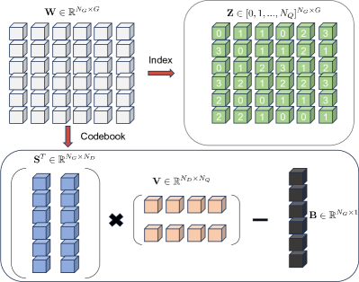
Figure 1: Illustration of low-rank codebook based quantization.

In AWQ [17] and GPTQ [9], the intervals between quantization values are equal, and hence it is not necessary to explicitly store the quantization codebook $\mathbf{C}$. More specifically, $\mathbf{C}$ can be represented by two vectors, a scaling vector $\mathbf{S}_{1}\in\mathbb{R}^{1\times N_{G}}$ and a fixed quantization point set (QPS) vector $\mathbf{V}_{1}\in\mathbb{R}^{1\times N_{Q}}$. $\mathbf{V}_{1}=[-1,-1+\frac{2}{2^{b}-1},\cdots,1-\frac{2}{2^{b}-1},1]$ is a uniformly spaced vector between $[-1,1]$. $\mathbf{S}_{1}$ can be adaptively obtained based on the weight matrix $\mathbf{W}$. The codebook is then obtained by computing the outer product of $\mathbf{S}_{1}$ and $\mathbf{V}_{1}$. Furthermore, to adapt to asymmetric weight distribution, a quantization offset $\mathbf{B}\in\mathbb{R}^{N_{G}\times 1}$ is introduced, with each group of weights having its own quantization offset. The final quantization codebook can be formulated as $\mathbf{C}=\mathbf{S}^{T}_{1}\mathbf{V}_{1}-\mathbf{B}$, which is a rank-one matrix. The storage cost for $\mathbf{S}_{1}$, $\mathbf{V}_{1}$ and $\mathbf{B}$ is $O(2*N_{G}+N_{Q})$, which is much lower than $O(N_{G}*N_{Q})$ for storing $\mathbf{C}$. Although rank-one codebook can reduce the storage cost, it has limited representation ability.

To improve the representation ability of the codebook, we propose to use a low-rank codebook for quantization. More specifically, we introduce two matrices: $\mathbf{S}=\left[\mathbf{S}_{1};\cdots;\mathbf{S}_{N_{D}}\right]\in\mathbb{R}^{N_{D}\times N_{G}}$, $\mathbf{V}=\left[\mathbf{V}_{1};\cdots;\mathbf{V}_{N_{D}}\right]\in\mathbb{R}^{N_{D}\times N_{Q}}$. The quantization codebook $\mathbf{C}$ is obtained as follows:

$$\mathbf{C}=\Phi(\mathbf{S},\mathbf{V},\mathbf{B})=\mathbf{S}^{T}\mathbf{V}-\mathbf{B}.$$ (3)

When $N_{D}>1$, the rank of the codebook $\mathbf{C}$ can be larger than one. When $N_{D}=1$, the codebook $\mathbf{C}$ degenerates to rank-one codebook as in existing methods [17, 9]. Hence, our LCQ has a stronger representation ability than existing methods, including existing rank-one codebook based methods as special cases. We will show that LCQ with $N_{D}>1$ will achieve better accuracy than LCQ with $N_{D}=1$ in Section 4. This verifies the stronger representation ability of our low-rank codebook compared to the rank-one codebook. Figure 1 shows the low-rank codebook with $N_{D}=2$.

3.2 Objective Function

As illustrated in Figure 1, LCQ starts with a pre-trained model and tries to find the optimal $\mathbf{S}$, $\mathbf{V}$ and $\mathbf{B}$ for minimizing the loss caused by quantization. We use the output reconstruction error of a Transformer block as the objective function like the methods in [1, 16, 35], which can make the parameters of a Transformer block be optimized simultaneously. Compared to the methods that use the output reconstruction error of a single linear layer as the objective function [9, 17], using the output reconstruction error of a Transformer block can avoid falling into local optima and prevent the accumulation of quantization error. A Transformer block in the Transformer-based models [30] typically contains the following linear layers: the query/key/value linear projection layers $\mathbf{W}^{qproj},\mathbf{W}^{kproj},\mathbf{W}^{vproj}$, the output projection layer $\mathbf{W}^{oproj}$ of the multi-head self-attention, and two linear layers $\mathbf{W}^{fc1}$ and $\mathbf{W}^{fc2}$ of the feed forward network. Therefore, the parameters of a Transformer block can be represented as $\mathcal{W}=\left[\mathbf{W}^{qproj},\mathbf{W}^{kproj},\mathbf{W}^{vproj},\mathbf{W}^{oproj},\mathbf{W}^{fc1},\mathbf{W}^{fc2}\right]$. Similarly, parameters $\mathcal{S},\mathcal{V},\mathcal{B}$ are used to represent all $\mathbf{S}$s, $\mathbf{V}$s, $\mathbf{B}$s within a Transformer block. We define the objective function to minimize the norm of the difference between the output with quantized weights and the output with unquantized weights in a Transformer block as follows:

$$\min_{\mathcal{S},\mathcal{V},\mathcal{B}} \sum_{i=1}^{N_{X}}||h(\tilde{\mathbf{X}}_{i},\mathcal{W}^{Q})-h(\mathbf{X}^{fp}_{i},\mathcal{W})||_{F}^{2}+||h(\tilde{\mathbf{X}}_{i},\mathcal{W}^{Q})-h(\tilde{\mathbf{X}}_{i},\mathcal{W})||_{F}^{2}.$$ (4)

where $h(\cdot)$ denotes the function of a Transformer block, and $N_{X}$ is the number of calibration samples. $\mathbf{X}^{fp}_{i}$ represents the feature with all previous blocks full precision and $\tilde{\mathbf{X}}_{i}$ represents the feature with all previous blocks quantized. $\mathcal{W}^{Q}=Q(\mathcal{W},\Phi(\mathcal{S},\mathcal{V},\mathcal{B}))$ represents the quantized weights in a Transformer block. $h(\tilde{\mathbf{X}}_{i},\mathcal{W}^{Q})$ represents the output feature of the Transformer block with all blocks quantized including this block. The objective function contains two items, one use $h(\mathbf{X}^{fp}_{i},\mathcal{W})$ as the reconstruction targets and another uses $h(\tilde{\mathbf{X}}_{i},\mathcal{W})$. Note that the quantization algorithm does not change the model weights $\mathbf{W}$ [28], in order to avoid forgetting existing knowledge. By fixing $\mathbf{W}$, we can also reduce the optimization overhead by reducing the number of parameters to be optimized.

3.3 Gradient-based Optimization

To solve the problem in (4), we propose a gradient-based optimization algorithm with strategies of gradient approximation for the quantization function, reparameterization of quantization parameters, and initialization of quantization parameters.

3.3.1 Gradient Approximation for Quantization Function

The $argmin(\cdot)$ operation in (1) will make the gradient unable to backpropagate through this function. This makes it challenging to learn the quantization codebook. We propose a gradient approximation strategy to address this issue.

As in N2UQ [19], we rewrite the quantization function into a form that adds up multiple segments, each corresponding to the interval between two adjacent quantization values. The form is as follows:

$$Q(W_{i,j},\mathbf{C}_{i}) =C_{i,\pi_{i}(1)}+\sum_{k=1}^{N_{Q}-1}\left(C_{i,\pi_{i}(k+1)}-C_{i,\pi_{i}(k)}\right)*\chi_{0.5}^{(k)}\left(\text{clip}\left(\frac{W_{i,j}-C_{i,\pi_{i}(k)}}{C_{i,\pi_{i}(k+1)}-C_{i,\pi_{i}(k)}},0,1\right)\right),$$ (5)

where $\pi_{i}(\cdot)$ is a sorting function that is responsible for sorting each row of the quantization codebook $\mathbf{C}$ in ascending order. The function $\text{clip}(\cdot,0,1)$ clips values outside $[0,1]$ to be within the $[0,1]$ range. The step function $\chi_{0.5}^{(k)}(x)$ is an element-wise function that discretizes weights, defined as follows:

$$\chi_{0.5}^{(k)}(x)=\begin{cases}1&\text{if }x>0.5,\text{ or }\left(x=0.5\text{ and }k\%2=1\right),\\ 0&\text{if }x<0.5,\text{ or }\left(x=0.5\text{ and }k\%2=0\right).\end{cases}$$ (6)

Here, we quantize critical values that are in the middle of two quantization values to the quantization value at the even position, corresponding to the condition $k\%2=0$ in (6). This avoids quantizing all critical values to the smaller/larger quantization value, preventing an overall bias in the quantization results. Furthermore, the elements which make $C_{i,\pi_{i}(k+1)}-C_{i,\pi_{i}(k)}$ equal zero, i.e., two adjacent quantization values are equal, can cause division by zero. To prevent such cases, we truncate values of $C_{i,\pi_{i}(k+1)}-C_{i,\pi_{i}(k)}$ that are less than $\epsilon$ to $\epsilon$. We can verify that the quantization function in (5) is equivalent to that in (2).

To address the issue that the gradient of the $\chi^{(k)}_{0.5}(x)$ is almost zero everywhere, we adopt the straight-through estimator (STE) approximation for the backward pass of the step function $\chi^{(k)}_{0.5}(x)$. This is defined as follows:

$$\frac{\partial\chi^{(k)}_{0.5}(x)}{\partial x}=\begin{cases}1&\text{if }0\leq x\leq 1,\\ 0&\text{otherwise}.\end{cases}$$ (7)

This means that the gradient for parameters within the $[0,1]$ interval is 1, while the gradient for parameters outside this interval is 0. The gradients for the rest of the operations in the quantization function $Q(\cdot)$ remain unchanged. By applying the chain rule, we can obtain $\frac{\partial\mathbf{W}^{Q}}{\partial\mathbf{S}},\frac{\partial\mathbf{W}^{Q}}{\partial\mathbf{V}},\frac{\partial\mathbf{W}^{Q}}{\partial\mathbf{B}}$ to optimize the quantization parameters $\mathbf{S},\mathbf{V},\mathbf{B}$ with gradient descent.

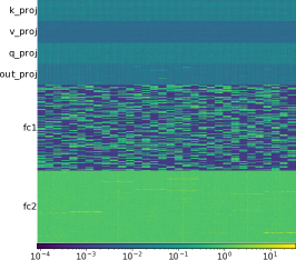
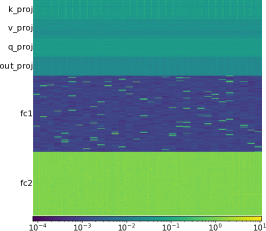
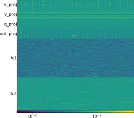
Figure 2: Visualization of $\mathcal{S}$ with AWQ, shown in the log scale. 3-bit quantization of a Transformer block in OPT-1.3B model. Left image: block 1; middle image: block 10; right image: block 20.

3.3.2 Reparameterization of Quantization Parameters

During the gradient descent process, we find it challenging to directly learn the scaling vectors $\mathcal{S}$ for all layers in a block. The main reason is that the values can vary significantly among different layers, and even within the same layer (e.g., in the fc1 layer), as shown in Figure 2. Directly learning $\mathcal{S}$ can result in excessive gradient updates for some weights while being too small for others, leading to difficulty in convergence. As in OmniQuant [28], we propose a reparameterization strategy to address the divergence issue caused by the large differences in $\mathcal{S}$ values. The reparameterization of $\mathbf{S}_{*,i}$ for the $i$th group of weights can be written as follows:

$$\mathbf{S}_{*,i} =g_{S}(\bar{\mathbf{S}}_{*,i},\mathbf{W}_{i})=\text{tanh}(\bar{\mathbf{S}}_{*,i})\left(\frac{\text{max}(\mathbf{W}_{i})-\text{min}(\mathbf{W}_{i})}{2}\right).$$ (8)

Here, different groups of weights have different reparameterization coefficients $\frac{\text{max}(\mathbf{W}_{i})-\text{min}(\mathbf{W}_{i})}{2}$, decoupling the weight range from $\mathbf{S}$. After reparameterization, the parameter to be optimized changes from $\mathbf{S}$ to $\bar{\mathbf{S}}$, which is relatively uniform across different layers and can improve the consistency among gradient magnitudes to facilitate convergence. The use of $\text{tanh}(\cdot)$ constrains the range of $\bar{\mathbf{S}}$, and subsequently prevents $\mathbf{S}$ from exceeding the maximum range of a group of weights.

For the reparameterization of the quantization offsets $\mathbf{B}$, we employ a similar method as that for the reparameterization of $\mathbf{S}$. But we need to solve an extra issue. More specifically, according to previous studies [17, 9], it is generally necessary to include the value $0$ in the set of quantized values. The main reason is that many weights in the model are close to $0$, and hence excluding $0$ from the quantized values would lead to significant quantization loss and severely degrade the accuracy of the final model. Assume the current offsets are $\mathbf{B}^{\prime}$. For the offsets $\mathbf{B}^{\prime}_{i}$ of the $i$th group, the reparameterized form is as follows:

$$\mathbf{B}_{i}^{\prime}=g_{S}(\bar{\mathbf{B}}_{i},\mathbf{W}_{i}).$$ (9)

A new substitute offset $\mathbf{B}_{i}$ must be recalculated in each optimization iteration based on $\mathbf{B}_{i}^{\prime}$, ensuring that the value $0$ is included in the codebook $\mathbf{C}_{i}$ when using $\mathbf{B}_{i}$. The offset calculation formula is as follows: $\mathbf{B}_{i}=Q(\mathbf{B}_{i}^{\prime},\mathbf{C}_{i}^{\prime})$, where $\mathbf{C}_{i}^{\prime}=\mathbf{S}_{i}^{T}\mathbf{V}$. This ensures that $\mathbf{B}_{i}$ is definitely an element of $\mathbf{C}_{i}^{\prime}$, and consequently, $0$ is assuredly an element of the quantization codebook $\mathbf{C}_{i}=\mathbf{S}_{i}^{T}\mathbf{V}-\mathbf{B}_{i}$.

We also reparameterize $\mathbf{V}$. As the range of weights has already been represented by $\mathbf{S}$, $\mathbf{V}$ does not need to represent the range of weights. We only need to use the $\text{tanh}(\cdot)$ function to constrain the range of $\mathbf{V}$ to be in $[-1,1]$:

$$\mathbf{V}=g_{V}(\bar{\mathbf{V}})=\text{tanh}(\bar{\mathbf{V}}).$$ (10)

Although the reparameterization strategy might result in a codebook in which the maximum range could exceed the maximum range of the group weights, we can constrain the initial maximum range of the codebook to be within the maximum range of the group weights during initialization. Subsequent optimization during gradient descent will then fine-tune the codebook within the vicinity of the initial values. The training and inference process of LCQ with reparameterization is shown in Figure 3.

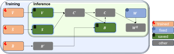
Figure 3: Training and inference process of LCQ with reparameterization.

3.3.3 Initialization of Quantization Parameters

We first get the initialization of $\mathbf{S},\mathbf{V},\mathbf{B}^{\prime}$. To get the initialization of reparameterization parameters, we calculate $\bar{\mathbf{S}}$, $\bar{\mathbf{V}}$, $\bar{\mathbf{B}}$ based on the inverse functions corresponding to (8),  (9), and (10).

We use the results of AWQ [17] to initialize rank1 quantization parameters. From the results of AWQ, we can obtain the parameters $\mathbf{S}_{1}$, $\mathbf{V}_{1}$, $\mathbf{B}^{\prime}$. Specifically, AWQ [17] optimizes the equivalent transformation parameters and the clipping parameters of each linear layer. For the equivalent transformation parameters, we apply the optimized equivalent transformation parameters of AWQ to scale the weights of each linear layer. For the clipping parameters, AWQ searches for the clipping parameters for each group of weights and then clips the weights. The range and mid-point of the clipped weights correspond to $\mathbf{S}_{1}$, $\mathbf{B}^{\prime}$. In addition, $\mathbf{V}_{1}$ is a vector with uniform interval, i.e., $\mathbf{V}_{1}=[-1,-1+\frac{2}{2^{b}-1},\cdots,1-\frac{2}{2^{b}-1},1]$ in AWQ.

For the remaining parameters, $\mathbf{S}_{r}(r\geq 2)$ is initialized to zero. $\mathbf{V}_{2}$ is initialized with equidistant points from a standard Gaussian distribution and $\mathbf{V}_{r}(r\geq 3)$ is initialized with sorted random values from $\text{Uniform}(-0.1,0.1)$. We get the initialization of $\bar{\mathbf{S}}_{r}(r\geq 2)$ and $\bar{\mathbf{V}}_{2}(r\geq 2)$ based on the inverse functions corresponding to (8) and (10). This ensures that the initialization of LCQ corresponds exactly to the results of AWQ, making the optimization process easier to converge to a good result.

3.4 Double Quantization

When $N_{D}>1$, LCQ will have more parameters than rank-one codebook based methods like AWQ, which will result in extra storage cost. To mitigate the extra storage cost associated with the enlarged $\mathbf{S}$ and $\mathbf{V}$, we adopt a double quantization strategy as in QLoRA [6] to further quantize $\mathbf{S}$ and $\mathbf{V}$. Taking $\mathbf{S}$ as an example, with double quantization, the optimization goal is to minimize the quantization error of $\mathbf{S}$:

$$\min_{\mathbf{S}^{dq},\mathbf{V}^{dq},\mathbf{B}^{dq}} ||Q_{\Phi(\mathbf{S}^{dq},\mathbf{V}^{dq},\mathbf{B}^{dq})}(\mathbf{S})-\mathbf{S}||^{2}_{2}.$$ (11)

Here, $\mathbf{S}^{dq},\mathbf{V}^{dq},\mathbf{B}^{dq}$ represent the parameters for double quantization. We adopt uniform quantization for double quantization. Like AWQ, we employ grid search to find the optimal $\mathbf{S}^{dq},\mathbf{V}^{dq},\mathbf{B}^{dq}$. More specifically, grid search is first used to identify the double quantization parameters for $\mathbf{S}$, which are then fixed. Subsequently, grid search is applied to determine the double quantization parameters for $\mathbf{V}$. As this process is independent of the input, the overall computational (time) cost is negligible.

The whole optimization procedure for LCQ is outlined in Algorithm 1. We sequentially quantize each Transformer block weights $\mathcal{W}_{b}$.

Algorithm 1 Optimization Procedure for LCQ

  Input: Pretrained LLM, calibration dataset $\{\mathbf{X}^{inp}_{i}\}_{i=1}^{N_{X}}$.

  Output: Quantization parameters for each Transformer block: $\mathcal{S},\mathcal{V},\mathcal{B}$.

  Initialize full-precision input features: $\{\mathbf{X}_{i}^{fp}\}_{i=1}^{N_{X}}=\{\mathbf{X}^{inp}_{i}\}_{i=1}^{N_{X}}$;

  for $b=1$ to $N_{block}$ do

     Initialize $\bar{\mathcal{S}},\bar{\mathcal{V}},\bar{\mathcal{B}}$ according to Section 3.3.3;

     for $t=1$ to $T$ do

        Sample a mini-batch from $\{\mathbf{X}^{fp}_{i}\}_{i=1}^{N_{X}}$;

        Sample the same mini-batch from $\{\tilde{\mathbf{X}}_{i}\}_{i=1}^{N_{X}}$;

        According to Section 3.3.2, $\mathcal{S},\mathcal{B}^{\prime},\mathcal{V}$ are computed from $\bar{\mathcal{S}},\bar{\mathcal{B}},\bar{\mathcal{V}}$. $\mathcal{B}$ is obtained from $\mathcal{B}^{\prime}$;

        Compute loss according to (4), and update parameters $\bar{\mathcal{V}},\bar{\mathcal{S}},\bar{\mathcal{B}}$ using gradient back-propagation with gradient approximation in (7);

     end for

     Perform double quantization for $\mathcal{S},\mathcal{V}$ according to (11), use grid search to find the optimal double quantization codebook, and save the parameters $\mathcal{S},\mathcal{V},\mathcal{B}$ of the current block;

     Compute the input features with all previous blocks full-precision for the next block: $\mathbf{X}_{i}^{fp}=h(\mathbf{X}^{fp}_{i},\mathcal{W}_{b}),\forall 1\leq i\leq N_{X}$;

     Compute the input features with all previous blocks quantized for the next block: $\tilde{\mathbf{X}}_{i}=h(\tilde{\mathbf{X}}_{i},\mathcal{W}_{b}^{Q}),\forall 1\leq i\leq N_{X}$;

  end for

4 Experiments

4.1 Experimental Setup

Calibration Dataset: As in AWQ [17], 128 samples randomly selected from Pile dataset [10] are used as the calibration dataset. The sequence length of each sample is 2048.

Quantization Hyperparameters: We adopt group quantization with two settings for group size: "G128" denotes a group size of 128, and "G-1" denotes that the group size is equal to the size of the channel. $N_{D}$ is set to 2 by default.

4.2 Comparison with Baselines

Table 1: Natural language generation ability on LLaMA, with perplexity as the metric. The best is shown in bold.

Config	Method	Retention Rate	LLaMA-7B	LLaMA-13B
WikiText2
fp16	-	1	5.68	5.09
W2 G128	AWQ [17]	0.134	12.90	9.73
	OmniQuant [28]	0.134	12.33	9.24
	LCQ	0.138	9.14	7.40
W3 G-1	AWQ [17]	0.188	8.43	6.37
	OmniQuant [28]	0.188	6.73	5.91
	LCQ	0.188	6.41	5.60
W3 G128	AWQ [17]	0.197	6.31	5.50
	OmniQuant [28]	0.197	6.30	5.53
	LCQ	0.202	6.17	5.49
C4
fp16	-	1	7.34	6.80
W2 G128	AWQ [17]	0.134	16.55	12.69
	OmniQuant [28]	0.134	14.79	11.60
	LCQ	0.138	11.44	9.76
W3 G-1	AWQ [17]	0.188	11.13	8.37
	OmniQuant [28]	0.188	8.73	7.67
	LCQ	0.188	8.35	7.42
W3 G128	AWQ [17]	0.197	8.17	7.34
	OmniQuant [28]	0.197	8.18	7.35
	LCQ	0.202	8.02	7.26

Table 2: Zero-shot performance of the quantized model for LLaMA-7B, with accuracy as the metric. The best is shown in bold.

Config	Method	PIQA	WinoGrande	ARC_easy
fp16	-	78.40	66.93	67.34
W2 G128	AWQ [17]	69.21	55.80	52.74
	OmniQuant [28]	66.92	53.20	49.37
	LCQ	72.36	60.30	59.13
W3 G128	AWQ [17]	76.33	65.19	65.07
	OmniQuant [28]	76.33	64.96	64.44
	LCQ	77.31	66.38	67.13

We choose AWQ [17] and OmniQuant [28] as baselines for comparison, because they are the most related works and have achieved state-of-the-art performance.

We first compare LCQ with baselines on the task of natural language generation, using OPT [38] and LLaMA [29] as pre-trained models. As in AWQ [17], we use three datasets WikiText2 [23], c4 [26] and PTB [22], with the perplexity (ppl) metric for evaluating the ability of the model to predict the next word (i.e., generative capability). The retention rate, defined as the rate between the remaining parameters to the original parameters, reflects the degree of model compression. The higher the retention rate is, the lower the degree of model compression will be. Table 1 shows the results on the three datasets, respectively. “fp16" denotes the original non-compressed model with 16-bit full-precision representation. “W2 G128” denotes a 2-bit weight quantization with a group size of 128. Other notations are defined similarly. We can find that LCQ achieves better accuracy than the baselines. In particular, in the case of 2-bit quantization, LCQ achieves significantly better accuracy than baselines. Furthermore, LCQ has a comparable retention rate with baselines, which means that the increase of $N_{D}$ brings a negligibly extra storage cost. We provide experiments on OPT models in the appendix.

We also compare LCQ with baselines on zero-shot tasks using three widely used datasets PIQA [2], WinoGrande [27] and ARC_easy [4]. Table 2 shows the accuracy of the quantized model for LLaMA-7B. We can find that LCQ achieves better accuracy than baselines on zero-shot tasks for all datasets. In particular, in the case of 2-bit quantization, the improvement is significant compared to baselines. The performance on zero-shot tasks also verifies that our LCQ method does not over-fit the calibration dataset and can maintain the generalization capability of the original model on zero-shot tasks.

5 Hyperparameter Sensitivity

First, we investigate the impact of different initialization methods for LCQ. We only perform experiments about the initialization for $\mathbf{V}_{2}$, and fix the initialization of other quantization parameters as described in Section 3.3.3. We compare three initialization methods: rand, uniform and normal. rand adopts sorted random values from $\text{Uniform}(-0.1,0.1)$ for initialization. uniform adopts the equidistant quantiles of a uniform distribution $\text{Uniform}(-1,1)$ for initialization. normal adopts the equidistant quantiles of a Gaussian distribution $\mathcal{N}(0,1)$  [6] for initialization. Figure 4(a) shows the results. We can find that different initialization methods do not have a significant impact on the performance. Hence, LCQ is robust to the initialization methods for $\mathbf{V}_{2}$. By default, we use normal for initialization to avoid extra hyperparameter settings.

We also study the impact of the number of training epochs. Figure 4(b) shows the result. We can find that 10 training epochs can achieve results comparable to those of 40 epochs. Hence, to expedite the training process, we adopt 10 training epochs by default.

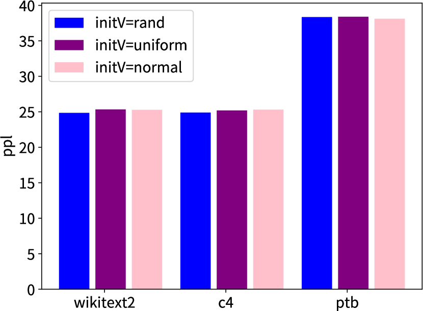
(a) Initialization for $\mathbf{V}$.

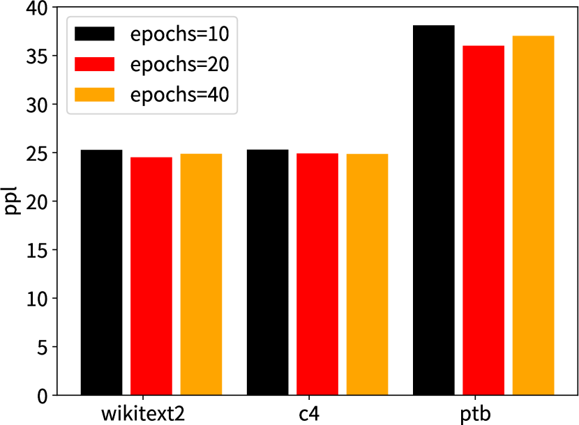
(b) Training epochs.

Figure 4: Hyperparameter sensitivity with “W2 G128" for OPT-1.3B.

The result about $N_{G}$ is in Figure 5(a). The smaller the $N_{G}$, the finer the quantization granularity. In particular, $N_{G}=\frac{N_{W}}{G}$ corresponds to the coarsest granularity, indicating that the whole linear layer corresponds a single $\mathbf{V}$. We can find that reducing $N_{G}$ can bring a slight improvement in model accuracy but also introduces some additional storage cost. To balance model accuracy and storage cost, we set $N_{G}=32$ by default.

The number of bits for double quantization will also affect the performance. Figure 5(b) shows the result. In particular, $\mathbf{S}_{1}$ is not quantized and kept in fp16, consistent with baseline methods. We can find that when using 4-bit quantization for $\mathbf{S}$ and 8-bit quantization for $\mathbf{V}$, the accuracy loss is minor or even negligible compared to methods without double quantization. However, when the number of quantization bits for $\mathbf{V}$ is reduced to 4, the accuracy loss is more significant. Hence, we use 4-bit quantization for $\mathbf{S}$ and 8-bit quantization for $\mathbf{V}$ by default. Double quantization is performed in groups of 16 elements by default.

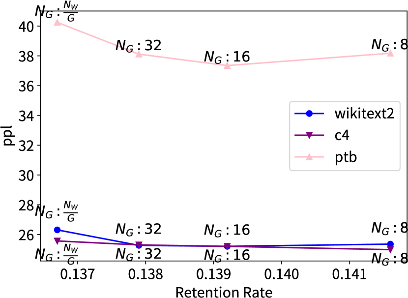
(a) $N_{G}$.

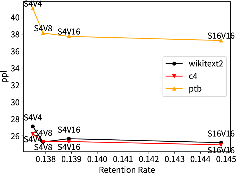
(b) Double quantization.

Figure 5: Hyperparameter sensitivity with “W2 G128" for OPT-1.3B.

We also explore the impact of $N_{D}$ on model performance, the result of which is shown in Table 3. We can find that compared to the results with $N_{D}=1$, the results with $N_{D}=2$ improve significantly, which verifies that increasing the rank of the codebook can lead to better accuracy. Further increasing $N_{D}$ can further improve the accuracy, but will also incur more storage cost. Hence, we set $N_{D}$ to 2 by default. Furthermore, we can also find that although the optimized parameters of AWQ are used to initialize $\mathbf{S}_{1},\mathbf{V}_{1},\mathbf{B}$ in LCQ, further learning (optimizing) these parameters can achieve better accuracy than fixing them. We provide more hyperparameter sensitivity analysis in the appendix.

Table 3: Perplexity on WikiText2 when using different $N_{D}$ and whether fixing $\mathbf{S}_{1},\mathbf{B},\mathbf{V}_{1}$, with “W2 G128" for OPT-1.3B.

$N_{D}$	Retention Rate	Fix	OPT-125M	OPT-1.3B
1	0.135	$\surd$	340.56	42.72
1	0.135	$\times$	88.89	28.50
2	0.137	$\surd$	76.98	27.09
2	0.138	$\times$	68.75	25.28
3	0.141	$\surd$	65.52	25.15
3	0.141	$\times$	61.49	24.82

6 Conclusion

In this paper, we propose a novel weight quantization method called LCQ for compressing LLMs. Experiments show that LCQ can outperform existing methods to achieve the best performance.

Limitations. We have only conducted experiments on uni-modal models and have not yet validated our method on multi-modal models. We will validate our method on multi-modal models in the future.

Appendix A Training Details

We perform experiments with PyTorch [25] on an RTX A6000 GPU card of 48GB memory, and use mixed-precision optimization to reduce the memory and computational cost during training. The ADAMW optimizer [21] is used, with an initial learning rate set to 0.01, and the weight decay factor set to 0. The learning rate is gradually reduced using a cosine annealing schedule [20] over a total of 10 training epochs. The batch size for training is set to 4, and gradient accumulation is employed to prevent memory overflow. The linear layer weights of all Transformer blocks are quantzied. The embedding layer and the output layer are not quantized.

Appendix B Experiments on OPT Models

Table 4 shows the experiments on OPT models.

Table 4: Natural language generation ability on OPT, with perplexity as the metric.

Config	Method	Retention Rate	OPT-125M	OPT-1.3B	OPT-6.7B
WikiText2
fp16	-	1	27.65	14.62	10.86
W2 G128	AWQ [17]	0.134	340.56	42.72	16.73
	OmniQuant [28]	0.134	117.25	34.69	17.15
	LCQ	0.138	68.75	25.28	15.49
W3 G-1	AWQ [17]	0.188	57.46	24.67	16.54
	OmniQuant [28]	0.188	41.50	18.85	12.98
	LCQ	0.188	36.88	17.54	11.96
W3 G128	AWQ [17]	0.197	35.99	16.41	11.36
	OmniQuant [28]	0.197	35.23	16.37	11.53
	LCQ	0.202	32.47	15.97	11.36
C4
fp16	-	1	26.56	16.07	12.71
W2 G128	AWQ [17]	0.134	246.47	40.63	19.55
	OmniQuant [28]	0.134	82.47	31.59	18.34
	LCQ	0.138	54.20	25.31	16.93
W3 G-1	AWQ [17]	0.188	48.83	24.55	17.79
	OmniQuant [28]	0.188	36.36	19.82	15.20
	LCQ	0.188	33.81	18.76	13.81
W3 G128	AWQ [17]	0.197	32.63	17.80	13.41
	OmniQuant [28]	0.197	31.92	17.69	13.43
	LCQ	0.202	30.12	17.30	13.30
PTB
fp16	-	1	38.99	20.29	15.77
W2 G128	AWQ [17]	0.134	516.64	73.33	25.95
	OmniQuant [28]	0.134	163.66	49.46	24.52
	LCQ	0.138	89.73	38.12	22.26
W3 G-1	AWQ [17]	0.188	86.42	34.65	21.56
	OmniQuant [28]	0.188	58.22	26.77	20.48
	LCQ	0.188	53.72	25.38	17.26
W3 G128	AWQ [17]	0.197	50.38	23.23	16.78
	OmniQuant [28]	0.197	48.78	22.85	16.76
	LCQ	0.202	46.75	22.40	16.65

References

- Bai et al. [2022] Haoli Bai, Lu Hou, Lifeng Shang, Xin Jiang, Irwin King, and Michael R. Lyu. Towards efficient post-training quantization of pre-trained language models. In NeurIPS, pages 1405–1418, 2022.
- Bisk et al. [2020] Yonatan Bisk, Rowan Zellers, Ronan Le Bras, Jianfeng Gao, and Yejin Choi. PIQA: reasoning about physical commonsense in natural language. In AAAI, pages 7432–7439, 2020.
- Brown et al. [2020] Tom B. Brown, Benjamin Mann, Nick Ryder, Melanie Subbiah, Jared Kaplan, Prafulla Dhariwal, Arvind Neelakantan, Pranav Shyam, Girish Sastry, Amanda Askell, Sandhini Agarwal, Ariel Herbert-Voss, Gretchen Krueger, Tom Henighan, Rewon Child, Aditya Ramesh, Daniel M. Ziegler, Jeffrey Wu, Clemens Winter, Christopher Hesse, Mark Chen, Eric Sigler, Mateusz Litwin, Scott Gray, Benjamin Chess, Jack Clark, Christopher Berner, Sam McCandlish, Alec Radford, Ilya Sutskever, and Dario Amodei. Language models are few-shot learners. In NeurIPS, pages 1877–1901, 2020.
- Clark et al. [2018] Peter Clark, Isaac Cowhey, Oren Etzioni, Tushar Khot, Ashish Sabharwal, Carissa Schoenick, and Oyvind Tafjord. Think you have solved question answering? try arc, the AI2 reasoning challenge. CoRR, abs/1803.05457, 2018.
- Dettmers et al. [2022] Tim Dettmers, Mike Lewis, Younes Belkada, and Luke Zettlemoyer. Llm.int8(): 8-bit matrix multiplication for transformers at scale. In NeurIPS, pages 30318–30332, 2022.
- Dettmers et al. [2023] Tim Dettmers, Artidoro Pagnoni, Ari Holtzman, and Luke Zettlemoyer. Qlora: Efficient finetuning of quantized llms. In NeurIPS, pages 10088–10115, 2023.
- Dettmers et al. [2024] Tim Dettmers, Ruslan Svirschevski, Vage Egiazarian, Denis Kuznedelev, Elias Frantar, Saleh Ashkboos, Alexander Borzunov, Torsten Hoefler, and Dan Alistarh. Spqr: A sparse-quantized representation for near-lossless LLM weight compression. In ICLR, 2024.
- Frantar and Alistarh [2022] Elias Frantar and Dan Alistarh. Optimal brain compression: A framework for accurate post-training quantization and pruning. In NeurIPS, pages 4475–4488, 2022.
- Frantar et al. [2023] Elias Frantar, Saleh Ashkboos, Torsten Hoefler, and Dan Alistarh. GPTQ: accurate post-training quantization for generative pre-trained transformers. In ICLR, 2023.
- Gao et al. [2021] Leo Gao, Stella Biderman, Sid Black, Laurence Golding, Travis Hoppe, Charles Foster, Jason Phang, Horace He, Anish Thite, Noa Nabeshima, Shawn Presser, and Connor Leahy. The pile: An 800gb dataset of diverse text for language modeling. CoRR, abs/2101.00027, 2021.
- Han et al. [2016] Song Han, Huizi Mao, and William J. Dally. Deep compression: Compressing deep neural network with pruning, trained quantization and huffman coding. In Yoshua Bengio and Yann LeCun, editors, ICLR, 2016.
- Kim et al. [2023] Jeonghoon Kim, Jung Hyun Lee, Sungdong Kim, Joonsuk Park, Kang Min Yoo, Se Jung Kwon, and Dongsoo Lee. Memory-efficient fine-tuning of compressed large language models via sub-4-bit integer quantization. In NeurIPS, pages 36187–36207, 2023.
- Kim et al. [2024] Sehoon Kim, Coleman Hooper, Amir Gholami, Zhen Dong, Xiuyu Li, Sheng Shen, Michael W. Mahoney, and Kurt Keutzer. Squeezellm: Dense-and-sparse quantization. In Proceedings of the International Conference on Machine Learning, 2024.
- Lee et al. [2024] Changhun Lee, Jungyu Jin, Taesu Kim, Hyungjun Kim, and Eunhyeok Park. OWQ: lessons learned from activation outliers for weight quantization in large language models. In AAAI, 2024.
- Li et al. [2024] Yixiao Li, Yifan Yu, Chen Liang, Pengcheng He, Nikos Karampatziakis, Weizhu Chen, and Tuo Zhao. Loftq: Lora-fine-tuning-aware quantization for large language models. In ICLR, 2024.
- Li et al. [2021] Yuhang Li, Ruihao Gong, Xu Tan, Yang Yang, Peng Hu, Qi Zhang, Fengwei Yu, Wei Wang, and Shi Gu. BRECQ: pushing the limit of post-training quantization by block reconstruction. In ICLR, 2021.
- Lin et al. [2023] Ji Lin, Jiaming Tang, Haotian Tang, Shang Yang, Xingyu Dang, and Song Han. AWQ: activation-aware weight quantization for LLM compression and acceleration. CoRR, abs/2306.00978, 2023.
- Liu et al. [2022a] Haotian Liu, Chunyuan Li, Qingyang Wu, and Yong Jae Lee. Visual instruction tuning. In NeurIPS, pages 34892–34916, 2022a.
- Liu et al. [2022b] Zechun Liu, Kwang-Ting Cheng, Dong Huang, Eric P. Xing, and Zhiqiang Shen. Nonuniform-to-uniform quantization: Towards accurate quantization via generalized straight-through estimation. In CVPR, pages 4932–4942, 2022b.
- Loshchilov and Hutter [2017] Ilya Loshchilov and Frank Hutter. SGDR: stochastic gradient descent with warm restarts. In ICLR, 2017.
- Loshchilov and Hutter [2019] Ilya Loshchilov and Frank Hutter. Decoupled weight decay regularization. In ICLR, 2019.
- Marcus et al. [1994] Mitchell P. Marcus, Grace Kim, Mary Ann Marcinkiewicz, Robert MacIntyre, Ann Bies, Mark Ferguson, Karen Katz, and Britta Schasberger. The penn treebank: Annotating predicate argument structure. In Human Language Technology, pages 114–119, 1994.
- Merity et al. [2017] Stephen Merity, Caiming Xiong, James Bradbury, and Richard Socher. Pointer sentinel mixture models. In ICLR, 2017.
- Oh et al. [2022] Sangyun Oh, Hyeonuk Sim, Jounghyun Kim, and Jongeun Lee. Non-uniform step size quantization for accurate post-training quantization. In ECCV, pages 658–673, 2022.
- Paszke et al. [2019] Adam Paszke, Sam Gross, Francisco Massa, Adam Lerer, James Bradbury, Gregory Chanan, Trevor Killeen, Zeming Lin, Natalia Gimelshein, Luca Antiga, Alban Desmaison, Andreas Köpf, Edward Z. Yang, Zachary DeVito, Martin Raison, Alykhan Tejani, Sasank Chilamkurthy, Benoit Steiner, Lu Fang, Junjie Bai, and Soumith Chintala. Pytorch: An imperative style, high-performance deep learning library. In NeurIPS, pages 8024–8035, 2019.
- Raffel et al. [2020] Colin Raffel, Noam Shazeer, Adam Roberts, Katherine Lee, Sharan Narang, Michael Matena, Yanqi Zhou, Wei Li, and Peter J. Liu. Exploring the limits of transfer learning with a unified text-to-text transformer. JMLR, 21:140:1–140:67, 2020.
- Sakaguchi et al. [2020] Keisuke Sakaguchi, Ronan Le Bras, Chandra Bhagavatula, and Yejin Choi. Winogrande: An adversarial winograd schema challenge at scale. In AAAI, pages 8732–8740, 2020.
- Shao et al. [2024] Wenqi Shao, Mengzhao Chen, Zhaoyang Zhang, Peng Xu, Lirui Zhao, Zhiqian Li, Kaipeng Zhang, Peng Gao, Yu Qiao, and Ping Luo. Omniquant: Omnidirectionally calibrated quantization for large language models. In ICLR, 2024.
- Touvron et al. [2023] Hugo Touvron, Thibaut Lavril, Gautier Izacard, Xavier Martinet, Marie-Anne Lachaux, Timothée Lacroix, Baptiste Rozière, Naman Goyal, Eric Hambro, Faisal Azhar, Aurélien Rodriguez, Armand Joulin, Edouard Grave, and Guillaume Lample. Llama: Open and efficient foundation language models. CoRR, abs/2302.13971, 2023.
- Vaswani et al. [2017] Ashish Vaswani, Noam Shazeer, Niki Parmar, Jakob Uszkoreit, Llion Jones, Aidan N. Gomez, Lukasz Kaiser, and Illia Polosukhin. Attention is all you need. In NeurIPS, pages 5998–6008, 2017.
- Wei et al. [2022] Xiuying Wei, Ruihao Gong, Yuhang Li, Xianglong Liu, and Fengwei Yu. Qdrop: Randomly dropping quantization for extremely low-bit post-training quantization. In ICLR, 2022.
- Wei et al. [2023] Xiuying Wei, Yunchen Zhang, Yuhang Li, Xiangguo Zhang, Ruihao Gong, Jinyang Guo, and Xianglong Liu. Outlier suppression+: Accurate quantization of large language models by equivalent and optimal shifting and scaling. CoRR, abs/2304.09145, 2023.
- Xiao et al. [2023] Guangxuan Xiao, Ji Lin, Mickaël Seznec, Hao Wu, Julien Demouth, and Song Han. Smoothquant: Accurate and efficient post-training quantization for large language models. In ICML, pages 38087–38099, 2023.
- Xu et al. [2024] Yuhui Xu, Lingxi Xie, Xiaotao Gu, Xin Chen, Heng Chang, Hengheng Zhang, Zhengsu Chen, Xiaopeng Zhang, and Qi Tian. Qa-lora: Quantization-aware low-rank adaptation of large language models. In ICLR, 2024.
- Yao et al. [2022] Zhewei Yao, Reza Yazdani Aminabadi, Minjia Zhang, Xiaoxia Wu, Conglong Li, and Yuxiong He. Zeroquant: Efficient and affordable post-training quantization for large-scale transformers. In Sanmi Koyejo, S. Mohamed, A. Agarwal, Danielle Belgrave, K. Cho, and A. Oh, editors, NeurIPS, pages 27168–27183, 2022.
- Yuan et al. [2023] Zhihang Yuan, Lin Niu, Jiawei Liu, Wenyu Liu, Xinggang Wang, Yuzhang Shang, Guangyu Sun, Qiang Wu, Jiaxiang Wu, and Bingzhe Wu. RPTQ: reorder-based post-training quantization for large language models. CoRR, abs/2304.01089, 2023.
- Zeng et al. [2023] Aohan Zeng, Xiao Liu, Zhengxiao Du, Zihan Wang, Hanyu Lai, Ming Ding, Zhuoyi Yang, Yifan Xu, Wendi Zheng, Xiao Xia, Weng Lam Tam, Zixuan Ma, Yufei Xue, Jidong Zhai, Wenguang Chen, Zhiyuan Liu, Peng Zhang, Yuxiao Dong, and Jie Tang. GLM-130B: an open bilingual pre-trained model. In ICLR, 2023.
- Zhang et al. [2022] Susan Zhang, Stephen Roller, Naman Goyal, Mikel Artetxe, Moya Chen, Shuohui Chen, Christopher Dewan, Mona T. Diab, Xian Li, Xi Victoria Lin, Todor Mihaylov, Myle Ott, Sam Shleifer, Kurt Shuster, Daniel Simig, Punit Singh Koura, Anjali Sridhar, Tianlu Wang, and Luke Zettlemoyer. OPT: open pre-trained transformer language models. CoRR, abs/2205.01068, 2022.