HOLISMOKES XIII: Strong-lens candidates at all mass scales and their environments from the Hyper-Suprime Cam and deep learning

We have performed a systematic search for galaxy-scale strong gravitational lenses using Hyper Suprime-Cam (HSC) imaging data, focusing on lenses in overdense environments. To identify these lens candidates, we exploit our residual neural network from HOLISMOKES VI, which is trained on realistic $gri$ mock-images as positive examples, and real HSC images as negative examples. Compared to our previous work, where we have successfully applied the classifier to around 62.5 million galaxies having $i$-Kron radius $\geq 0.8\arcsec$, we now lower the $i$-Kron radius limit to $\geq 0.5\arcsec$. This results in an increase by around 73 million sources to more than 135 million images. During our visual multi-stage grading of the network candidates, we now also inspect simultaneously larger stamps ($80\arcsec\times 80\arcsec$) to identify large, extended arcs cropped in the $10\arcsec\times 10\arcsec$ cutouts and classify additionally their overall environment. Here, we also re-inspect our previous lens candidates with $i$-Kron radii $\geq 0.8\arcsec$ and classify their environment. Using these 546 visually identified lens candidates, we further define various criteria by exploiting extensive and complementary photometric redshift catalogs, to select the candidates in overdensities. In total, we identified 24 grade-A and 138 grade-B candidates with either spatially-resolved multiple images or extended, distorted arcs in the new sample. Furthermore, combining our different techniques, we identify in total 237/546 lens candidates in a cluster-like or significant overdense environment, containing only 49 group- or cluster-scale re-discoveries. These results demonstrate the feasibility of downloading and applying neural network classifiers to hundreds of million cutouts, necessary in the upcoming era of big data from deep, wide-field imaging surveys like Euclid and the Rubin Observatory Legacy Survey of Space and Time, while leading to a sample size that can be visually inspected by humans. These deep learning pipelines, with false-positive rates of $\sim 0.01$%, are very powerful tools to identify such rare galaxy-scale strong lensing systems, while also aiding in the discovery of new strong lensing clusters.

1 Introduction

Strong gavitational lensing systems, both on galaxy scales and cluster scales, are very powerful tools to probe the Universe’s properties in several aspects such as the study of the nature and distribution of dark matter (e.g., Schuldt et al., 2019; Shajib et al., 2021; Wang et al., 2022), and of high-redshift systems (e.g., Lemon et al., 2018; Shu et al., 2018; Vanzella et al., 2021; Meštrić et al., 2022). Furthermore, strong lensing systems with time variable objects, like a quasar or supernova (SN), enable the measurement of the Hubble constant $H_{0}$ and the geometry of the Universe as proposed by Refsdal (1964). While so far mostly galaxy-scale systems with lensed quasars are exploited for this (e.g., by the H0LiCOW and TDCOSMO collaborations, see e.g., Wong et al., 2020; Birrer et al., 2020; Shajib et al., 2022), it was also demonstrated on cluster scales (e.g., Acebron et al., 2022a, b) where the mass distribution is significantly more complicated. Extending this systematically to lensed SNe, is one of the main scientific goals of our Highly Optimized Lensing Investigations of Supernovae, Microlensing Objects, and Kinematics of Ellipticals and Spirals (HOLISMOKES Suyu et al., 2020) program. To date, only very few lensed SNe were found and in fact, only two systems so far, called SN Refsdal and SN H0pe which are lensed by galaxy clusters (Kelly et al., 2015a, b), have sufficiently precise time delays to enable measurements of the Hubble constant and the geometry of the universe (Grillo et al., 2018, 2020; Kelly et al., 2023; Grillo et al., 2024; Frye et al., 2023; Pascale et al., 2024). A third lensed supernova by a galaxy cluster (Pierel et al., 2024), named SN Encore whose galaxy previously hosted SN Requiem (Rodney et al., 2021), was discovered in November 2023 and analyses are ongoing to use this system for time-delay cosmography.

With recently started and upcoming wide-field imaging surveys such as the Rubin Observatory Legacy Survey of Space and Time (LSST; Ivezic et al., 2008) from the ground, complemented by the Euclid (Laureijs et al., 2011) and Roman (Green et al., 2012) satellites from space, the amount of astronomical imaging data sets is expected to increase significantly in the optical and near-infrared wavelength range in the next years. Thanks to their runtime and performance in image pattern recognition, supervised deep learning (DL) techniques such as convolutional neural networks (CNNs Lecun et al., 1998) are playing a significant role in the analysis of these data sets. Once trained, these networks can be applied to millions or billions of image cutouts within an acceptable amount of time. Beside exploiting supervised CNNs for photometric redshift estimation (D’Isanto & Polsterer, 2018; Schuldt et al., 2021b; John William et al., 2023; Jones et al., 2023), modelling strong galaxy-scale lenses (e.g., Hezaveh et al., 2017; Pearson et al., 2019, 2021; Schuldt et al., 2021a, 2023a, 2023b), detecting dark matter substructure Tsang et al. (2024), estimating structural parameters of galaxies (Tuccillo et al., 2018; Tohill et al., 2021; Li et al., 2022), or classifying them according to their morphology (Dieleman et al., 2015; Walmsley et al., 2022), DL became the state of the art technique for lens classification (Metcalf et al., 2019). Although sharing the same baseline of relying on DL, there have been various projects that are targeting different image sets (e.g., Jacobs et al., 2017, 2019; Cañameras et al., 2020; Canameras et al., 2023; Savary et al., 2022) and possibly limiting to particular lens samples, such as lensed quasars (e.g., Andika et al., 2023), systems with high lens redshift (e.g., Shu et al., 2022), or being within a cluster environment (Angora et al., 2023). These CNNs are complementing previous non-DL algorithms (e.g., Chan et al., 2015; Sonnenfeld et al., 2018; Shu et al., 2016) with generally better classification performance (Metcalf et al., 2019).

In Cañameras et al. (2021, herafter C21), we presented a CNN trained on realistic mock images and applied it to $gri$ multiband images from the Hyper-Suprime Cam Subaru Strategic Program (HSC-SSP; Aihara et al., 2018), complemented with detailed performance test presented by Canameras et al. (2023). Avoiding any strict cuts on the catalog level, we applied it to 62.5 million image stamps from the HSC Wide layer, which correspond to a lower limit on the $i$-band Kron radius of $0.8\arcsec$. This is possible thanks to a false-positive rate (FPR) of $\sim 0.01$%. From the 9 651 resulting systems, corresponding to 0.015% of the input catalog, we identified through our visual inspection 88 secure (grade A) and 379 probable (grade B) lens candidates. Given the high success rate, we present in this work new lens candidates by lowering the limit on the $i$-Kron radius to 0.5″, which gives us additionally $\sim$ 73 million image stamps.

Since the scope of C21 was specifically on detecting new galaxy-scale lenses, we neglected, as commonly done, possible group- or cluster-scale lensing features during our visual inspection. However, as reported in C21 already, our network was able to recover also group- and cluster-scale lenses. Therefore, we adjust our visual inspection strategy and report this time also specifically lenses in a significantly overdense environment such as a galaxy cluster by inspecting larger cutouts ($80\arcsec$ on a side). This is complemented by a re-inspection of the lens candidates from C21 to classify their environment.

While the deep-learning based identification of galaxy-scale lenses in the field is well explored, only Angora et al. (2023) developed so far a network to identify galaxy-scale lenses in galaxy clusters, which was trained on $4\arcsec\times 4\arcsec$ high-resolution image cutouts in known clusters. In contrast, we use $\sim 12\arcsec\times 12\arcsec$ ground-based image stamps from HSC, allowing the network to analyze also the close environment and identify extended arcs caused by a galaxy cluster. Furthermore, we apply it to any astronomical source targeted by HSC with $i$-Kron radius above 0.5″, which enable the identification of new galaxy-scale lenses in the field as well.

Using the visually identified lens candidates in overdensities, and lens candidates near known galaxy clusters, we define and test several selection criteria for their identification. These criteria are based on the photometric redshift distribution of their surrounding objects. Here we focus specifically on our lens candidates, as lenses are already on average in slightly overdense environments (e.g., Wells et al., 2024). We exploit three complementing photometric redshift catalogs providing more than a hundred million measurements in the targeted footprint. Thanks to the expected accurate and large photometric redshift catalog from ongoing and upcoming wide-field imaging surveys, these criteria can be used to identify lenses in significant overdensities, while also identifying galaxy clusters independent of their lensing nature.

The paper is organized as follows. We first introduce the overall procedure in Sect. 2. Sect. 3 describes our visual inspection strategy and the identified lens candidates. In Sect. 4 we highlight our analysis on the lens environment and in Sect. 5 we finally conclude our findings. Following C21, we adopt the flat concordant $\Lambda$CDM cosmology with $\Omega_{\text{M}}$ $=1-\Omega_{\Lambda}$ $=0.308$ (Planck Collaboration et al., 2016), and with $H_{0}=72\,\text{km\,s}^{-1}\,\text{Mpc}^{-1}$ (Bonvin et al., 2017).

2 Methodology

We make use of the residual neural network presented by C21, and therefore refer the interested reader to that publication, as well as to Canameras et al. (2023), for details. In the following, we give a short summary of the network architecture, the ground truth data set, and the training procedure.

2.1 Network architecture

Over time, neural networks got more and more powerful thanks to, for instance, increasing training set sizes, more powerful computing techniques allowing to train deeper networks, and their broad applicability. Consequently, different network architectures and algorithms were developed to optimize the performance. While the architecture for image processing tasks are overall still following the original setup of a simple CNN (Lecun et al., 1998), which consists of multiple convolutional layers followed by a number of fully connected layers, the depth of the network significantly increased over time. In particular, the residual neural network (ResNet) concept (He et al., 2016a) introduces so-called skip-connections (preactivated bottleneck residual units in He et al., 2016b) to allow deep CNNs while avoiding vanishing gradient to optimize also the first layers well and keeping the computational costs at an acceptable level. Such ResNets have obtained excellent results on the ImageNet Large Scale Visual Recognition Challenge 2015 (He et al., 2016a). In the recent past, these ResNets were also used for lens finding (e.g., Lanusse et al., 2018; Li et al., 2020; Huang et al., 2021) and outperformed classical CNNs from the lens finding challenge Metcalf et al. (2019).

We used a ResNet whose architecture setup is based on the ResNet-18 architecture (He et al., 2016a). It is composed of eight ResNet blocks with each 2 convolutional layers, batch normalization and a ReLu activation function. These layers are followed by a fully connected layer with 16 neurons, before the last layer with a single neuron that outputs a score $p$ in the range [0,1] through to a sigmoid activation function.

2.2 Ground truth dataset

Our binary classification network is trained and validated on a set of images composed by 40 000 positive and 40 000 negative examples. As positive examples, we used simulated images of galaxy-scale lenses that are based on real HSC $gri$ images of luminous red galaxies (LRGs). Following the procedure described in Cañameras et al. (2020) and Schuldt et al. (2021b), we added to those LRG images arcs simulated with Glee (Suyu & Halkola, 2010; Suyu et al., 2012) from galaxy images of the Hubble Ultra Deep Field (Inami et al., 2017) as background sources. We adopted here a singular isothermal ellipsoid profile and estimated the ellipticity based on that of the light distribution. The Einstein radius was inferred from the corresponding velocity dispersion and redshift measurement taken from the Sloan Digital Sky Survey program (SDSS, Abolfathi et al., 2018). Since it is important to have a uniform distribution in the training set, we increase the fraction of systems with wide image separations to obtain a sample with uniform Einstein radius distribution in the range 0.75″to 2.5″, and use a similar fraction of quadruply- and doubly- imaged systems.

This data set is complemented with negative examples, containing mostly spirals from Tadaki et al. (2020), isolated LRGs, and random galaxies with similar proportions. These were selected from random sky positions of the HSC Wide footprint to mitigate impact from small-scale and depth variations.

2.3 Training procedure

The data set described in Sect. 2.2 was split up into 80% training and 20% validation. The test sample and performance tests are summarized in Sect. 2.4.

After randomly initialization, the network was trained over 100 epochs, while the network was saved at the epoch with the minimal binary-entropy loss on the validation set. We used mini-batch stochastic gradient descent with 128 images per batch, a learning rate of 0.0006, a weight decay of 0.001, and a momentum of 0.9. In each epoch all images were randomly shifted by up to $\pm 5$ pixels in $x$ and $y$ direction to improve generalization.

2.4 Performance tests

We carried out several performance test of the network based on a test set with HSC Wide PDR2 images as described in detail by Canameras et al. (2023). In short, the completeness was tested with grade A or B galaxy-scale lenses from the Survey of Gravitationally-lensed Objects in HSC Imaging (SuGOHI, Sonnenfeld et al., 2018, 2019, 2020; Wong et al., 2020; Chan et al., 2020; Jaelani et al., 2020a, 2021, hereafter SuGOHI sample). We excluded from this sample systems with high image separations (Einstein radius $\geq 4\arcsec$), that are not matching our training data and consequently are expected to be likely missed.

On the other hand, the FPR was estimated with a set of non-lens galaxies from the COSMOS field Scoville et al. (2007) by ensuring all known lenses and candidate lenses listed in the MasterLens database, Faure et al. (2011), Pourrahmani et al. (2018), as well as systems from the SuGOHI sample, are excluded. Using a threshold of $p\geq 0.1$, we obtained a completeness above 50% on galaxy-scale systems and a FPR $\leq 0.01\%$. The obtained Receiver Operating Characteristic curve is shown in Fig. 2 of C21.

Given our focus this time on lenses at all mass scales, approximately 25% of the grade A and B SuGOHI group and cluster-scale lenses are recovered in our list of candidates. This relatively low recovery rate is understandable given that the network is trained specifically on galaxy-scale systems but highlights the possibility of new group- and cluster lens discoveries with this ResNet, as well as generally with automated algorithms.

3 Lens grading

The following section describes the visual inspection and grading procedure of the network candidates with $i$-Kron radii between $0.5\arcsec$ and $0.8\arcsec$. We further discuss the outcome and the effect of the individual steps, which help to plan future visual inspection strategies.

3.1 Network candidates

The trained network was applied to all $\sim$72 million images from the HSC Wide layer showing objects with an $i$-band Kron radius between 0.5″and 0.8″, complementing the sample from C21 targeting objects with $i$-band Kron radii $\geq 0.8\arcsec$. Based on the tests in C21, we considered all 11 816 objects ($\sim$ 0.016% of the input catalog) with a network score $p\geq 0.1$ as network candidates. The obtained fraction is comparable to that achieved in C21, which indicates that the network has the capability to also handle objects that appear smaller or with some offset to the image center, as several times the central object is one of the possible lensed images or a compact object near the candidate lens system.

3.2 First cleaning through visual inspection

As in previous lens search studies, including C21, these network candidates have a significant fraction of false positives such that we carry out a visual inspection of these systems using pre-generated $gri$-color images. These images were inspected first by one person to exclude obvious non-lenses, reducing the candidates to 1 475 systems. These false positives had mostly a low network score, such that a higher threshold would reduce the FPR significantly. However, in this case we would miss several possible lens candidates. In fact, a threshold of 0.11 instead of 0.1 would already exclude 12 grade B candidates of which 8 are already known (see Table 1 and Sect. 3.4), justifying the relatively low threshold.

Table 1: High-confidence lens candidates with ResNet scores $p\geq 0.1$, and average grades $G\geq 1.5$ from visual inspection.

Name	RA [deg]	Dec [deg]	$p$	$G$	$\sigma_{\text{G}}$	$z$	OD${}_{\text{lit}}$	OD${}_{\text{vis}}$	OD${}_{\text{z}}$	$N_{\text{max}}$	$z_{\text{low}}$	$N_{\text{tot}}$	References
(1)	(2)	(3)	(4)	(5)	(6)	(7)	(8)	(9)	(10)	(11)	(12)	(13)	(14)
HSCJ2331$+$0037	$352.87702$	$0.62594$	$0.91$	$3.00$	$0.00$	0.56	Y	N	N	18	0.56	724	W18 C21
HSCJ2305$-$0002	$346.34029$	$-0.03658$	$1.00$	$3.00$	$0.00$	0.49	N	N	Y	22	0.62	609	W18 C21
HSCJ0128$+$0038	$22.47583$	$0.63363$	$0.14$	$2.88$	$0.33$	0.61	Y	N	Y	25	0.78	546	C21 S22
HSCJ0925$+$0017	$141.43748$	$0.28450$	$0.20$	$2.88$	$0.33$	1.36	Y	N	Y	24	0.76	833	J20 C21
HSCJ2332$+$0038	$353.12887$	$0.63939$	$0.98$	$2.75$	$0.43$	0.61	N	N	N	20	0.80	779	W18 C21
⋮	⋮	⋮	⋮	⋮	⋮	⋮	⋮	⋮	⋮	⋮	⋮	⋮	⋮

Note. Column description: (1) Source name, (2) right ascension (J2000), (3) declination (J2000), (4) network score, (5) average grade from our visual inspection, (6) dispersion among the eight graders, (7) photometric redshift of the recentered lens galaxy candidate from our combined catalog based on DEmP (Hsieh & Yee, 2014), Mizuki (Tanaka et al., 2018), and NetZ (Schuldt et al., 2021a), flag on the overdensity (OD) based on (8) Literature (Oguri, 2014; Oguri et al., 2018; Wen & Han, 2018, 2021), (9) visual inspection, and (10) the photometric redshift analysis, (11) absolute height of photo-$z$ distribution, (12) photo-$z$ lower bound, (13) total number of photo-$z$ in considered area, and (14) references of their previous discovery with M16 for More et al. (2016), D17 for Diehl et al. (2017), S18 for Sonnenfeld et al. (2018), W18 for Wong et al. (2018), H19 for Huang et al. (2019), P19 for Petrillo et al. (2019), Ca20 for Cao et al. (2020) H20 for Huang et al. (2020) J20 for Jaelani et al. (2020b), S20 for Sonnenfeld et al. (2020), C21 for Cañameras et al. (2021), R22 for Rojas et al. (2022), S22 for Shu et al. (2022), A23 for Andika et al. (2023), J23 for Jaelani et al. (2023), and ML for the master lens catalog http://admin.masterlens.org.

3.3 Multiple grader inspection

According to Rojas et al. (2023, hereafter R23), the visual inspection should be done by at least six individual persons to ensure stable average grades, while the accuracy is still dropping with increasing number of graders (compare Fig. 15 in R23). To reduce the images that need to be inspected, we carry out a multi-step inspection with eight individuals.

During the visual grading, we inspected $gri$-color images with a size of $10\arcsec\times 10\arcsec$ to grade the central object and its close surrounding, showing possible arcs. In addition, which is done for the first time, we look at larger images to classify their environment. Since 80″correspond to about 0.5 Mpc at $z=0.5$, a typical lens cluster redshift (e.g., Bergamini et al., 2021; Acebron et al., 2022a, b; Schuldt et al., 2024), this size ensure that extended cluster-scale arcs remain within the images and enough of the cluster environment is included while keeping the astronomical objects visible on the inspector’s screen. Therefore, our grading tool shows, in addition to three $10\arcsec\times 10\arcsec$ $gri$-color images with different filter scalings, also three $80\arcsec\times 80\arcsec$ cutouts centered at the small image stamp, again with different stretching factors.

In addition to the new possibility of voting for an overdensity during visual inspection, we incorporated in our grading tool the option to indicate if the lens galaxy is not the central object. This is particularly important in our case, as multiple lens candidates are centered at their possible arc or at a neighbouring objects given our selection criteria on more compact objects. We correct these offsets manually after grading for the most probable lenses reported in Table 1.

Round #1: As initial step, we conducted a calibration round containing 200 systems inspected by everyone. This is crucial to calibrate the expectations and discuss individual systems. We assigned to each system, as already in previous studies, a grade between zero and three, corresponding to not a lens, possible lens, probable lens, and definite lens. The grades from round #1 are not taken into account for the final lens candidate compilation shown in Table 1.

Round #2: After calibration, we split ourselves into two teams of each four people. Each team graded 825 of the 1 475 network candidates, with an overlap of 175 random systems (hereafter, the overlap sample) that are graded by both teams for comparison. As expected from R23, we observe significant differences between the individual grades, but also between the two teams. In Fig. 1, we show a normalized histogram of the number of grades 0 (not a lens) and grades 1 (possible lens), for all possible team combinations of the graders. We clearly see significant differences between a single grader and a team of two people. Significant scatter remains for three and four graders, which is in agreement with results from R23, recommending to average over at least six individual grades.

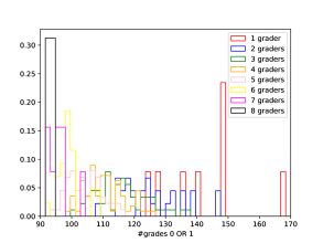
Figure 1: Normalized histograms showing the distribution of 0 and 1 grades assigned in round #2 to network candidates from the overlap sample, containing 175 systems. We show all possible team combinations of the eight graders and only count systems that received a 0 or 1 by all graders of a particular team combination. Significant scatter is observed for small teams, which is expected and in agreement with R23.

As mentioned above, we also observed differences between the two teams. This is shown in Fig. 2, where we plot the average grade $G_{\text{A}}$ from team A on the $x$-axis and the average grade $G_{\text{B}}$ from team B on the $y$-axis. Although each team contains four individuals, we see a tendency towards lower grades from team A. However, we note that the sample only contains 175 systems and thus, particularly at higher grades, the statistic is relatively poor. In detail, the top panel of Fig. 2 shows the results from round #2, while the middle panel displays the results from round #3, and the bottom panel from round #4, which we describe below.

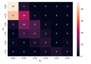
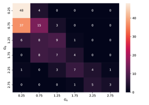
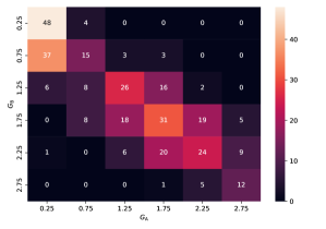
Figure 2: Comparison between average grades from team A ($x$-axis) and team B ($y$-axis), containing each four graders, from round #2 (top), round #3 (middle), with each 175 systems (overlap sample), and round #4 (bottom), containing all 327 objects that got 8 grades.

Round #3: Both teams re-inspected the systems with strong discrepancy in the provided grades within each team (standard deviation above 0.75). Cases with high dispersion in visual grades often show ambiguous blue arcs that could either be lensed arcs from background galaxies (without clear counter-images), spiral arms, or tidal features. From Fig. 2, we see a slight improvement from round #2 to #3 in terms of agreement in the average grades from the two teams, while the discrepancy remains.

Round #4: To increases the number of examiners per object as recommended by R23, each team graded the systems with average grade above 1 obtained by the complementary team. This excludes a significant fraction of additional false-positive candidates and systems with not very clear lensing features. This consequently reduces the time required for round #4, while ensuring a stable average grade from eight inspectors per relevant object. We explicitly chose a slightly lower threshold than for the final compilation (see Sect. 3.4) to counterbalance the observed discrepancy and the effect of lower number of inspectors.

In the bottom panel of Fig. 2, we show the differences between the final average grades for all 327 systems that obtained eight grades, again split into the previous two teams for comparison. This highlights the good agreement between both teams for the relevant systems and shows a stabilization for more than four graders.

3.4 Final lens candidate compilation

Finally, we compute for all 1 475 systems the average grade, where grades from earlier rounds are superseded by newer grades regardless of their value. As in previous lens search projects (e.g., Cañameras et al., 2020; Shu et al., 2022), we define grade A lens candidates as systems with final average grade $G\geq 2.5$ and grade B systems with $2.5>G\geq 1.5$. In total, we identify finally 24 grade-A candidates and 138 grade-B candidates. We further correct for 75 out of 162 lens candidates manually the lens center, as we identified here a significant offset. This is crucial to correctly identify and monitor these lenses in the future. These candidates were selected often through an arc falling into our $i$-Kron range, such that the possible lens galaxy may have a higher $i$-Kron radius. All, if needed re-centered, lens candidates are shown in Fig. 3 and Fig. 6, and listed in Table 1. The number of identified systems is slightly lower than obtained in previous programs (e.g., Jacobs et al., 2019; Cañameras et al., 2021; Shu et al., 2022) but still comparable with network based searches (e.g., Rojas et al., 2022; Savary et al., 2022) and depend also on the used image survey and its footprint size. This is most likely due to the sample selection of low $i$-Kron radii systems, containing galaxies with lower mass, consequently acting less likely as strong lenses or creating too small Einstein radii to be identified with the resolution from HSC (0.168″/pixel).

Figure 3: Re-centered color-image stamps ($12\arcsec\times 12\arcsec$) of identified grade-A lens candidates using HSC $gri$ multi-band imaging data. On the top of each panel we list the ResNet scores $p$, and the average grades $G$ of eight graders, where $\geq 2.5$ corresponds to grade A, from visual inspection. In the bottom we list the candidate name, displayed in white for new candidates, light blue if previously detected as grade C lens candidate, and green if previously known grade A or B lens candidate. Given the numerous lens search projects exploiting HSC data, only our grade-B systems, which are shown in Fig. 6, include new identification highlighted additionally with orange boxes. All systems with their coordinates and further details such as the lens environment are listed in Table 1.

3.5 Comparison with known systems

From our lens candidates listed in Table 1, 118 candidates are already known based on the current SLED (C. Lemon, private communication, May 2024) and our HOLISMOKES compilation. From these systems, 12 and 60 from our grade A and B sample, respectively, match the grade from the literature. In contrast, 12 and 21 systems from our grade A and B sample, respectively, obtained higher grades than before. On the other hand, 8 published systems with grade A belong to the grade B class according to our grading. We further miss 62 systems during the visual inspection of the 1475 network candidates, of which 43 are published with grade C (mostly from the SuGOHI sample). Missing grade C candidates is expected as we compile only for grade A and B systems. In total, this shows that a strict grading is difficult as it also depends on the inspected image quality/resolution, filter amount, and possibly detection algorithm (especially for non-DL techniques such as modelling). However, it shows that the expectation on the lensing features are broadly consistent over the years and grading teams.

The relatively high number of known systems is expected since the HSC data set was targeted by multiple lens search projects, complemented by several other lens searches with data in the same footprint. Therefore, to reduce the number of systems during visual inspection, we propose to exclude previously graded systems in the future, regardless of their previous grade, unless the target sample, the data quality (e.g., high resolution images from Euclid), or the detection algorithm (e.g., including lens deblending or modeling) changed significantly. However, a downside of excluding previously visually classified objects is that one cannot carry out a consistency check with grades from the literature as done above.

4 Environment analysis

Since the surrounding mass distribution of a galaxy-scale lens influences the lensing effect of that system, the characteristics of the environment are crucial and need to be taken into account when building a strong lens mass model. In addition, galaxy-cluster lenses are modeled completely differently from galaxy-scale lenses and are particularly difficult to identify with autonomous algorithm because of their size, complexity, and peculiarity. However, cluster lenses have several advantages over galaxy-scale lenses, such as significantly longer time delays and higher magnifications, enabling several complementary studies to galaxy-scale systems. For these reasons, beside enlarging the sample to which we apply the network, we conduct an analysis of the lens candidate environment, which we describe in the following.

Here we also re-consider our detected lens candidates from C21, and combine them with our new sample. This leads, after excluding duplicates, to a total of 546 grade A or grade B lens candidates, based on our visual inspection described in Sect. 3 and C21.

4.1 Comparison with the literature

As a first step, we crossmatch our network candidates with a large sample of galaxy clusters without known strong lensing features from the literature. In detail, we first use the catalog from Oguri (2014), containing 71 743 clusters identified by the Camira code using data from the SDSS Data Release 8 (York et al., 2000; Aihara et al., 2011) covering $\sim$11960 deg² of the sky, including the whole footprint of HSC-SSP DPR2 and thus all our lens candidates. This algorithm is based on stellar population synthesis models to predict colours of red sequence galaxies at a given redshift. The identified clusters cover a redshift range between 0.1 and 0.6 (Oguri, 2014). This code was also directly applied to HSC data, resulting in 1 921 galaxy clusters presented by Oguri et al. (2018). Since HSC images are significantly deeper than those from SDSS, this catalog extend the redshift range up to $z\sim 1$.

We complement both Camira catalogs with 1 959 galaxy clusters detected by Wen & Han (2018) using SDSS and Wide-field Infrared Survey Explorer (WISE) data, and 21 661 galaxy clusters published by Wen & Han (2021) exploiting HSC-SSP and WISE data. Wen & Han (2018, 2021) target specifically the high redshift range $z\geq 0.7$, complementing ideally identifications by the Camira algorithm. The identifications in Wen & Han (2021) are based on photometric redshifts obtained from the 7-band photometric data from HSC and SDSS WISE using a nearest-neighbour algorithm.

This sums up to a total of more than 100 000 galaxy clusters with most systems in the targeted HSC Wide area. Thanks to the two complementary techniques, it also covers a large redshift range, ensures a roughly equal distribution over the HSC footprint, and reduced selection biases.

The cross-match radius is selected based on the size of known lensing clusters. For instance, Schuldt et al. (2024) present 308 securely identified cluster members of the lensing cluster MACS J1149.5+2223, which therefore is one of the largest sample of cluster members. They are distributed over an area of around 160″on a side, mostly limited by the area of available high-resolution imaging data. Therefore, to also include systems with significant offset to the BCG, we adopt a radius of 100″. This size corresponds to $\sim 0.65$ Mpc at the lens cluster redshift of MACS J1149.5+2223, and roughly to the peak of the distribution of the reported R500 radii in Wen & Han (2021). The distribution of the reported R500 radii starts at around 0.36 Mpc, which corresponds to 100″ at a redshift of 0.25, and the distribution drops significantly until $\sim 0.8$ Mpc, which equals to 100″ at $z=0.9$, supporting our selected radius of 100″.

In this way, we identify 174 grade A or B lens candidates to be located within 100″ from a galaxy cluster centroid listed in the galaxy cluster catalogs. Out of these 174 systems, 63 systems are more than 50″away from the reported cluster center, and only 44 are part of the SuGOHI group- or cluster scale lens sample. We indicate the possible overdense environment from the literature with OD${}_{\text{lit}}$ in Table 1 and Table 2 for the newly identified systems and those from C21, respectively. These cluster identifications are used in the following as a reference.

Table 2: High-confidence lens candidates reported by C21 and not listed in Table 1, now with analysis of their environment.

Name	RA	Dec	$p$	$G$	$\sigma_{\text{G}}$	$z$	OD${}_{\text{lit}}$	OD${}_{\text{vis}}$	OD${}_{\text{z}}$	$N_{\text{max}}$	$z_{\text{low}}$	$N_{\text{tot}}$	References
(1)	(2)	(3)	(4)	(5)	(6)	(7)	(8)	(9)	(10)	(11)	(12)	(13)	(14)
HSCJ1004$-$0031	$151.21577$	$-0.52915$	$0.17$	$3.00$	$0.00$	$1.05$	Y	Y	N	17	0.50	513	C21 A23
HSCJ1224$-$0042	$186.20954$	$0.704233$	$0.28$	$3.00$	$0.00$	$0.38$	Y	Y	Y	23	0.50	791	J20 P19 C21
HSCJ1434$-$0056	$218.72664$	$-0.94963$	$0.94$	$3.00$	$0.00$	$0.76$	Y	Y	Y	27	0.72	820	S18 J20 C21 J23
HSCJ0102$+$0158	$15.65975$	$1.98276$	$0.12$	$3.00$	$0.00$		N	N	N	10	0.74	259	C21 A23
HSCJ0238$-$0545	$39.57340$	$-5.76603$	$0.72$	$3.00$	$0.00$	$1.77$	N	N	N	8	0.86	357	S18 C21
⋮	⋮	⋮	⋮	⋮	⋮	⋮	⋮	⋮	⋮	⋮	⋮	⋮	⋮

Note. Column description: (1) Source name, (2) right ascension (J2000), (3) declination (J2000), (4) network score, (5) average grade from our visual inspection, (6) dispersion among the eight graders, (7) photometric redshift from our combined catalog based on DEmP (Hsieh & Yee, 2014), Mizuki (Tanaka et al., 2018), and NetZ (Schuldt et al., 2021a), flag on the overdensity (OD) based on (8) galaxy cluster catalogs (Oguri, 2014; Oguri et al., 2018; Wen & Han, 2018, 2021), (9) visual inspection, and (10) photometric redshift, (11) absolute height of photo-$z$ distribution, (12) photo-$z$ lower bound, (13) total number of photo-$z$ in considered area, and (14) references of their previous discovery, apart from (C21), with S13 for Sonnenfeld et al. (2013), G14 for Gavazzi et al. (2014), M16 for More et al. (2016), D17 for Diehl et al. (2017), S18 for Sonnenfeld et al. (2018), W18 for Wong et al. (2018), H19 for Huang et al. (2019), P19 for Petrillo et al. (2019), Ch20 for Chan et al. (2020), Ca20 for Cao et al. (2020) L20 for Li et al. (2020), J20 for Jaelani et al. (2020b), S20 for Sonnenfeld et al. (2020), C21 for Cañameras et al. (2021), T21 for Talbot et al. (2021), R22 for Rojas et al. (2022), S22 for Shu et al. (2022), A23 for Andika et al. (2023), J23 for Jaelani et al. (2023), and ML for the master lens catalog http://admin.masterlens.org.

4.2 By visual inspection of the environment

As described in Sec. 3, we visually inspected all the newly detected network candidates. Here we consider, beside $10\arcsec\times 10\arcsec$ cutouts that are a typical size used for visual inspection, also stamps of $80\arcsec\times 80\arcsec$ in size, showing the larger environment (see Fig. 4). Since all galaxies that belong to a galaxy cluster are located at nearly the same redshift, the so-called cluster redshift, and mostly containing galaxies with similar morphologies, they appear with similar colors in the images, easing the identification of galaxy clusters based on color images. Consequently, large magnitude catalogs were used in the past to help identifying galaxy clusters (e.g., Oguri, 2014). Instead, we introduced in our grading tool a new possibility to also indicate a cluster environment, which increases the required human time for the visual inspection very little, while gaining additional crucial information on the lens candidate. To simplify the identification, we focus on overdensities in general, which means we report also several group-scale lenses as well as lenses with high number of lines-of-sight companions possibly not physically associated with the lens candidate. As a consequence, and in analogy to the observed differences in the grades, we also observe here some differences in the votes. In the rare case that only one or two graders (out of four or eight, see Sect. 3) indicated an overdensity, the lens candidate was inspected once more with the focus on the environment for a final decision. Lens candidates with more than two votes are directly indicated to be in a cluster-like environment based on the visual inspection. This is noted as OD${}_{\text{vis}}$ in Table 1 and Table 2.

Figure 4: New grade A or grade B lens candidates visually identified to be on group- or cluster-scale, excluding known group- or cluster lenses from the SuGOHI sample. Each panel is $80^{\prime\prime}\times 80^{\prime\prime}$, and the insert on the top-left shows the $12^{\prime\prime}\times 12^{\prime\prime}$ cutout analysed by the ResNet. The lens name is given in the bottom of each panel, in cyan if listed in the galaxy cluster catalogs, and otherwise white. Furthermore, the network score, average grade, and number of cluster votes during visual inspection is given in the top (first row), in orange if listed by C21, in cyan if listed in this work, and white if in both. This is followed by the photo-$z$ characteristics $N_{\text{max}},z_{\text{low}},N_{\text{tot}}$, and $N_{\text{frac}}$ (second row), and $N_{\text{peak5}}$, $A_{\text{peak5}}$, $N_{\text{peak10}}$, and $A_{\text{peak10}}$ (third row), colored green or red if passing or not passing the final limits (No. 46 in Table 3), respectively. We note that lens candidates from C21 were only inspected by a single person for group/cluster environment classifications and thus have all only one vote. The figure continues in Appendix B.

Furthermore, one person re-inspected the network candidates reported in C21 regarding the environment, while we adopt the assigned average grades $G$ on the lensing nature from C21 directly. This leads to an identification of additionally 47 (out of 467 grade A or B lens candidates in C21) to be in a significantly overdense environment, which are listed in Table 2. By combining both samples and removing duplicates, the new candidates from Sect. 3 and those from C21, we visually identify, out of 546 grade A or B lens candidates, 84 to be in an overdense environment. Interestingly, from these 84 lens candidates, only 31 are reported in the SuGOHI group- and cluster-scale sample. This demonstrated the necessity of further analysis of the lens environment to enlarge the sample of group- and cluster-scale lenses. In addition, only 54 of the 84 identified systems are reported in the considered galaxy cluster catalogs, and only 27 in both, the SuGOHI and the galaxy cluster catalogs. This highlights that several lens candidates recently identified with deep learning classifiers were lacking on the information of their environment.

4.3 By photometric redshifts

As a further characterization of the environment from our new lens candidates, as well as the lens candidates from C21, we obtain for each candidate the photometric redshift (hereafter photo-$z$) distribution within a given area, as detailed below. This analysis goes therefore beyond the analysis of simple magnitude catalogs and will be broadly applicable to upcoming wide field surveys such as Euclid and LSST, with large and accurate photo-$z$ catalogs (e.g., Schmidt et al., 2020; Euclid Collaboration et al., 2020, 2024). We elaborate possible criteria such as the height of the distribution peak and the sum of all objects with available photo-$z$ value in the considered field to identify additional lenses in overdensities. In addition, the peak of the photo-$z$ distribution indicates the cluster redshift and helps to determine whether the lens galaxy belongs to the cluster.

For this analysis, we use photometric redshift catalogs from three different and complementary codes that were broadly applied to objects from the HSC wide area. In detail, these codes are Mizuki (Tanaka et al., 2018), a template fitting code with Bayesian priors, DEmP (Hsieh & Yee, 2014), a hybrid machine-learning code based on polynomial fitting, and NetZ (Schuldt et al., 2021a), a CNN based code that infer the photo-$z$ values directly from the HSC $grizy$-image stamps. All three catalogs obtained very good performance against spectroscopic redshifts, and contain, after excluding duplicates defined by a distance of less than two pixels ($\leq 0.336\arcsec$), each on the order of several ten million redshifts. In case of duplicates, we took the simple average of all, typically two, photo-$z$ values as well as the coordinates, and considered them as a single object. This ensures that we do not artificially overestimate the density of objects in a given area and expect to reduce the effect of catastrophic outliers. The relatively low threshold of only two pixels is chosen to not introduce wrong photo-$z$ values through averaging. We further follow Schuldt et al. (2021a), and limit the catalogs to a photo-$z$ range $0<z<5$, given that the trustworthiness of photo-$z$ values significantly decreases with increasing redshift. By combining the three catalogs, we finally obtain a photo-$z$ catalog containing more than 115 million redshifts in the targeted footprint area.

Based on the size of known lensing clusters (compare Sect. 4.1), we consider all objects within a $200\arcsec$ $\times$ $200\arcsec$ field, centered at the lens candidate in the analysis. Since the cluster member galaxies are typically within a redshift bin of around 0.03 to 0.06 (see e.g., Bergamini et al., 2021, 2023; Acebron et al., 2022a, b; Schuldt et al., 2024), we create a photo-$z$ histogram for all lens candidates with a redshift bin width of $0.02$. However, we note that the range of the cluster members in our distributions is broadened given the photo-$z$ uncertainties. We show the histograms of two lens candidates, one visually identified to be in an overdense environment and one not, in Fig. 7 as example.

For the selection of overdensities, we first exploit the extracted photo-$z$ distributions directly, and define eight criteria. First, since a higher peak of the photo-$z$ distribution indicates a higher concentration of galaxies at a similar redshift, we introduce the absolute height of the photo-$z$ distribution peak $N_{\text{max}}$ as a criterion. The second criterion is the total amount of objects in the adopted field $N_{\text{tot}}$, indicating the density of the field in general. The third criteria is the ratio $N_{\text{frac}}=N_{\text{max}}/N_{\text{tot}}$, indicating the concentration of systems at the given redshift bin compared to the whole distribution. Since, as noted above, we expect a galaxy cluster to cover multiple neighbouring redshift bins, we further introduce $N_{\text{peak5}}$ and $N_{\text{peak10}}$, which gives the number of bins next to $N_{\text{max}}$ that exceeds 5 or 10 counts, respectively. These are complemented with the criteria $A_{\text{peak5}}$ and $A_{\text{peak10}}$, which give the sum of objects within $N_{\text{peak5}}$ and $N_{\text{peak10}}$, respectively. These seven criteria rely on the fact that the different and complementary photometric redshift algorithms were applied broadly to the same footprint of the network candidates. These criteria are highlighted in the photo-$z$ histograms shown in Fig. 7.

Finally, to exclude distributions significantly affected by photo-$z$ outliers, we also use the lower bound $z_{\text{low}}$ of the redshift bin corresponding to $N_{\text{max}}$ as a selection criterion. In addition, based on the SuGOHI sample, galaxy clusters at very low redshift ($z\lesssim 0.1$) or very high redshift ($z\gtrsim 1$) are very unlikely to create strong lensing effects detectable in HSC images, our target sample. In the case where two redshift bins have the exact same number of systems $N_{\text{max}}$, we use the lower redshift bin value as $z_{\text{low}}$ since higher photometric redshifts are normally less accurate and consequently a peak at higher redshift might be just due to photo-$z$ outliers than indicating a real galaxy cluster. We note that this choice does not affect our first three criteria at all, and that a combination of these criteria is crucial, as detailed below.

Since we are only interested in the characterization of strong lensing systems, and because galaxy-scale lenses are in general located in fields with higher density (e.g., Wells et al., 2024), we limit the analysis to our 546 visually identified lens candidates. Nonetheless, we run the photo-$z$ analysis on the whole set of network candidates with $p\geq 0.1$, as well as 10,000 random positions in the HSC footprint, for comparison and consistency checks. This sample of 546 lens candidates contains, based on the considered galaxy cluster catalogs and the visual inspection, 174 and 84 systems, respectively, in a significantly overdense environment.

We show in Fig. 5 the distribution obtained for our eight introduced selection criteria. This highlights the difference between systems in overdensities (blue and green) compared to those in the field (orange and magenta), and consequently the effectiveness of our selection criteria. For comparison, we show in gray the inferred values from 10,000 randoms positions in the HSC footprint. This confirms also findings from Wells et al. (2024) that lenses are in general in overdense environments.

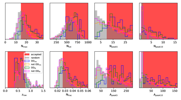
Figure 5: Normalized histograms of our eight introduced selection criteria. We distinguish between lens candidates visually identified to be in an overdensity (blue) or through the galaxy cluster catalogs (green), compared to those not in an overdensity (orange and magenta, respectively). We further show, for comparison, the distribution from 10,000 random positions in gray. Following the F1 criterion, we highlight the parameter range indicating overdensities in red (shaded regions for criteria No. 46 in Table 3), which demonstrates that a combination of these different criteria is crucial to gain good performance (see also No. 50 to 54 in Table 3).

We now set different thresholds for these eight criteria and test them against the visually identified lens candidates. While it is possible that we missed some clusters during our visual inspection, and we expect the considered galaxy cluster catalogs to be not complete, we treat these samples now as the ground truth for inferring the best thresholds for our eight introduced criteria. This allows us to define the true-positive (TP) and false-positive (FP) rates, which we list for a representative selection of different limits in Table 3. For comparison, we include as No. 0 the full sample sizes of lens candidates (indicated by selection cuts that all candidates passes the criteria by definition).

Table 3: Comparison of true-positive (TP) and false-positive (FP) rates for different selection criteria using the photometric redshift distributions around the 546 grade A or B lens candidates. We distinguish between lens candidates classified as clusters during visual inspection (see Sect. 4.2) and based on galaxy catalogs (Oguri, 2014; Oguri et al., 2018; Wen & Han, 2018, 2021). Without photo-$z$ selection (see No. 0), we visually identified 84 lens candidates to be in an overdense environment, while 174 lens candidates are located closer than $100\arcsec$ from a known galaxy cluster. We highlight No. 46 in bold, which has the selection criteria cuts that are the best according to the F1${}_{\text{tot}}$ statistic.

No.	Criteria									visual insp.		Literature		F1 statistics
	$N_{\text{max}}$	$z_{\text{low}}$	$z_{\text{low}}$	$N_{\text{tot}}$	$N_{\text{frac}}$	$N_{\text{peak5}}$	$A_{\text{peak5}}$	$N_{\text{peak10}}$	$A_{\text{peak10}}$	TP	FP	TP	FP	F1${}_{\text{vis}}$	F1${}_{\text{lit}}$	F1${}_{\text{tot}}$
0	$\geq 0$	$\geq 0$	$\leq\inf$	$\geq 0$	$\geq 0$	$\geq 0$	$\geq 0$	$\geq 0$	$\geq 0$	84	462	174	372	0.210	0.483	0.358
1	$\geq 15$	$\geq 0.1$	$\leq 1.0$	$\geq 400$	$\geq 0.025$	$\geq 0$	$\geq 0$	$\geq 0$	$\geq 0$	68	188	119	137	0.425	0.553	0.499
2	$\geq 15$	$\geq 0.1$	$\leq 1.0$	$\geq 400$	$\geq 0.026$	$\geq 0$	$\geq 0$	$\geq 0$	$\geq 0$	67	167	115	119	0.450	0.564	0.516
3	$\geq 15$	$\geq 0.1$	$\leq 1.0$	$\geq 400$	$\geq 0.027$	$\geq 0$	$\geq 0$	$\geq 0$	$\geq 0$	64	146	109	101	0.467	0.568	0.526
4	$\geq 15$	$\geq 0.1$	$\leq 1.0$	$\geq 500$	$\geq 0.025$	$\geq 0$	$\geq 0$	$\geq 0$	$\geq 0$	65	170	111	124	0.435	0.543	0.497
5	$\geq 15$	$\geq 0.1$	$\leq 1.0$	$\geq 500$	$\geq 0.026$	$\geq 0$	$\geq 0$	$\geq 0$	$\geq 0$	64	149	107	106	0.462	0.553	0.515
6	$\geq 15$	$\geq 0.1$	$\leq 1.0$	$\geq 500$	$\geq 0.027$	$\geq 0$	$\geq 0$	$\geq 0$	$\geq 0$	61	128	101	88	0.482	0.556	0.526
7	$\geq 15$	$\geq 0.1$	$\leq 0.8$	$\geq 400$	$\geq 0.025$	$\geq 0$	$\geq 0$	$\geq 0$	$\geq 0$	68	161	113	116	0.464	0.561	0.520
8	$\geq 15$	$\geq 0.1$	$\leq 0.8$	$\geq 400$	$\geq 0.026$	$\geq 0$	$\geq 0$	$\geq 0$	$\geq 0$	67	144	109	102	0.487	0.566	0.533
9	$\geq 15$	$\geq 0.1$	$\leq 0.8$	$\geq 400$	$\geq 0.027$	$\geq 0$	$\geq 0$	$\geq 0$	$\geq 0$	64	124	103	85	0.508	0.569	0.544
10	$\geq 15$	$\geq 0.1$	$\leq 0.8$	$\geq 500$	$\geq 0.025$	$\geq 0$	$\geq 0$	$\geq 0$	$\geq 0$	65	144	106	103	0.476	0.554	0.521
11	$\geq 15$	$\geq 0.1$	$\leq 0.8$	$\geq 500$	$\geq 0.026$	$\geq 0$	$\geq 0$	$\geq 0$	$\geq 0$	64	127	102	89	0.502	0.559	0.535
12	$\geq 15$	$\geq 0.1$	$\leq 0.8$	$\geq 500$	$\geq 0.027$	$\geq 0$	$\geq 0$	$\geq 0$	$\geq 0$	61	107	96	72	0.526	0.561	0.547
13	$\geq 17$	$\geq 0.1$	$\leq 1.0$	$\geq 400$	$\geq 0.025$	$\geq 0$	$\geq 0$	$\geq 0$	$\geq 0$	63	139	106	96	0.474	0.564	0.526
14	$\geq 17$	$\geq 0.1$	$\leq 1.0$	$\geq 400$	$\geq 0.026$	$\geq 0$	$\geq 0$	$\geq 0$	$\geq 0$	62	128	105	85	0.488	0.577	0.540
15	$\geq 17$	$\geq 0.1$	$\leq 1.0$	$\geq 400$	$\geq 0.027$	$\geq 0$	$\geq 0$	$\geq 0$	$\geq 0$	60	114	100	74	0.504	0.575	0.546
16	$\geq 17$	$\geq 0.1$	$\leq 1.0$	$\geq 500$	$\geq 0.025$	$\geq 0$	$\geq 0$	$\geq 0$	$\geq 0$	61	130	102	89	0.478	0.559	0.526
17	$\geq 17$	$\geq 0.1$	$\leq 1.0$	$\geq 500$	$\geq 0.026$	$\geq 0$	$\geq 0$	$\geq 0$	$\geq 0$	60	119	101	78	0.494	0.572	0.540
18	$\geq 17$	$\geq 0.1$	$\leq 1.0$	$\geq 500$	$\geq 0.027$	$\geq 0$	$\geq 0$	$\geq 0$	$\geq 0$	58	105	96	67	0.511	0.570	0.546
19	$\geq 17$	$\geq 0.1$	$\leq 0.8$	$\geq 400$	$\geq 0.025$	$\geq 0$	$\geq 0$	$\geq 0$	$\geq 0$	63	120	101	82	0.510	0.566	0.543
20	$\geq 17$	$\geq 0.1$	$\leq 0.8$	$\geq 400$	$\geq 0.026$	$\geq 0$	$\geq 0$	$\geq 0$	$\geq 0$	62	112	100	74	0.521	0.575	0.553
21	$\geq 17$	$\geq 0.1$	$\leq 0.8$	$\geq 400$	$\geq 0.027$	$\geq 0$	$\geq 0$	$\geq 0$	$\geq 0$	60	98	95	63	0.541	0.572	0.560
22	$\geq 17$	$\geq 0.1$	$\leq 0.8$	$\geq 500$	$\geq 0.025$	$\geq 0$	$\geq 0$	$\geq 0$	$\geq 0$	61	111	97	75	0.517	0.561	0.543
23	$\geq 17$	$\geq 0.1$	$\leq 0.8$	$\geq 500$	$\geq 0.026$	$\geq 0$	$\geq 0$	$\geq 0$	$\geq 0$	60	103	96	67	0.529	0.570	0.553
24	$\geq 17$	$\geq 0.1$	$\leq 0.8$	$\geq 500$	$\geq 0.027$	$\geq 0$	$\geq 0$	$\geq 0$	$\geq 0$	58	89	91	56	0.550	0.567	0.560
25	$\geq 15$	$\geq 0.1$	$\leq 0.8$	$\geq 400$	$\geq 0.025$	$\geq 7$	$\geq 50$	$\geq 1$	$\geq 15$	67	149	110	106	0.479	0.564	0.528
26	$\geq 15$	$\geq 0.1$	$\leq 0.8$	$\geq 400$	$\geq 0.025$	$\geq 7$	$\geq 70$	$\geq 1$	$\geq 15$	66	145	109	101	0.480	0.568	0.531
27	$\geq 15$	$\geq 0.1$	$\leq 0.8$	$\geq 400$	$\geq 0.025$	$\geq 1$	$\geq 15$	$\geq 2$	$\geq 26$	66	128	106	88	0.512	0.576	0.550
28	$\geq 15$	$\geq 0.1$	$\leq 0.8$	$\geq 400$	$\geq 0.025$	$\geq 1$	$\geq 15$	$\geq 2$	$\geq 30$	66	117	100	82	0.534	0.562	0.551
29	$\geq 15$	$\geq 0.1$	$\leq 0.8$	$\geq 400$	$\geq 0.027$	$\geq 7$	$\geq 50$	$\geq 1$	$\geq 15$	63	114	101	76	0.523	0.575	0.554
30	$\geq 15$	$\geq 0.1$	$\leq 0.8$	$\geq 400$	$\geq 0.027$	$\geq 7$	$\geq 70$	$\geq 1$	$\geq 15$	62	95	100	73	0.561	0.576	0.570
31	$\geq 15$	$\geq 0.1$	$\leq 0.8$	$\geq 400$	$\geq 0.027$	$\geq 1$	$\geq 15$	$\geq 2$	$\geq 26$	62	100	97	65	0.549	0.577	0.566
32	$\geq 15$	$\geq 0.1$	$\leq 0.8$	$\geq 400$	$\geq 0.027$	$\geq 1$	$\geq 15$	$\geq 2$	$\geq 30$	61	91	92	60	0.565	0.564	0.565
33	$\geq 15$	$\geq 0.1$	$\leq 0.8$	$\geq 400$	$\geq 0.025$	$\geq 10$	$\geq 50$	$\geq 1$	$\geq 15$	65	122	99	88	0.518	0.548	0.536
34	$\geq 15$	$\geq 0.1$	$\leq 0.8$	$\geq 400$	$\geq 0.025$	$\geq 10$	$\geq 70$	$\geq 1$	$\geq 15$	65	122	99	88	0.518	0.548	0.536
35	$\geq 15$	$\geq 0.1$	$\leq 0.8$	$\geq 400$	$\geq 0.025$	$\geq 7$	$\geq 50$	$\geq 1$	$\geq 26$	65	121	103	83	0.520	0.572	0.551
36	$\geq 15$	$\geq 0.1$	$\leq 0.8$	$\geq 400$	$\geq 0.025$	$\geq 7$	$\geq 70$	$\geq 1$	$\geq 26$	64	119	102	81	0.518	0.571	0.550
37	$\geq 15$	$\geq 0.1$	$\leq 0.8$	$\geq 400$	$\geq 0.027$	$\geq 10$	$\geq 50$	$\geq 1$	$\geq 15$	61	96	93	64	0.552	0.562	0.558
38	$\geq 15$	$\geq 0.1$	$\leq 0.8$	$\geq 400$	$\geq 0.027$	$\geq 10$	$\geq 70$	$\geq 1$	$\geq 15$	61	79	93	64	0.598	0.562	0.576
39	$\geq 15$	$\geq 0.1$	$\leq 0.8$	$\geq 400$	$\geq 0.027$	$\geq 7$	$\geq 50$	$\geq 1$	$\geq 26$	61	95	95	61	0.555	0.576	0.567
40	$\geq 15$	$\geq 0.1$	$\leq 0.8$	$\geq 400$	$\geq 0.027$	$\geq 7$	$\geq 70$	$\geq 1$	$\geq 26$	60	95	94	60	0.548	0.573	0.563
41	$\geq 15$	$\geq 0.1$	$\leq 0.8$	$\geq 470$	$\geq 0.027$	$\geq 10$	$\geq 50$	$\geq 1$	$\geq 15$	61	92	91	62	0.562	0.557	0.559
42	$\geq 15$	$\geq 0.1$	$\leq 0.8$	$\geq 470$	$\geq 0.027$	$\geq 10$	$\geq 70$	$\geq 1$	$\geq 15$	61	76	91	62	0.607	0.557	0.576
43	$\geq 15$	$\geq 0.1$	$\leq 0.8$	$\geq 470$	$\geq 0.027$	$\geq 7$	$\geq 50$	$\geq 1$	$\geq 26$	60	91	92	59	0.558	0.566	0.563
44	$\geq 15$	$\geq 0.1$	$\leq 0.8$	$\geq 470$	$\geq 0.027$	$\geq 7$	$\geq 70$	$\geq 1$	$\geq 26$	59	91	91	58	0.551	0.563	0.559
45	$\geq$15	$\geq$ 0.1	$\leq$0.8	$\geq$470	$\geq$0.027	$\geq$10	$\geq$100	$\geq$1	$\geq 15$	61	75	91	58	0.610	0.563	0.580
46	$\geq$15	$\geq$0.1	$\leq$0.8	$\geq$470	$\geq$0.027	$\geq$10	$\geq$120	$\geq$1	$\geq$15	58	67	87	49	0.614	0.561	0.581
47	$\geq 15$	$\geq 0.1$	$\leq 0.8$	$\geq 470$	$\geq 0.027$	$\geq 7$	$\geq 100$	$\geq 1$	$\geq 26$	59	77	86	50	0.590	0.555	0.569
48	$\geq 15$	$\geq 0.1$	$\leq 0.8$	$\geq 470$	$\geq 0.027$	$\geq 7$	$\geq 120$	$\geq 1$	$\geq 26$	57	67	82	42	0.606	0.550	0.572
49	$\geq 15$	$\geq 0.1$	$\leq 0.8$	$\geq 400$	$\geq 0.027$	$\geq 5$	$\geq 50$	$\geq 2$	$\geq 26$	62	98	96	64	0.554	0.575	0.566
50	$\geq 15$	$\geq 0.1$	$\leq 0$	$\geq 0$	$\geq 0$	$\geq 0$	$\geq 0$	$\geq 0$	$\geq 0$	76	284	147	213	0.358	0.551	0.466
51	$\geq 0$	$\geq 0.1$	$\leq 0$	$\geq 470$	$\geq 0$	$\geq 0$	$\geq 0$	$\geq 0$	$\geq 0$	79	364	151	292	0.312	0.489	0.409
52	$\geq 0$	$\geq 0.1$	$\leq 0$	$\geq 0$	$\geq 0.027$	$\geq 0$	$\geq 0$	$\geq 0$	$\geq 0$	70	227	127	372	0.388	0.377	0.381
53	$\geq 0$	$\geq 0.1$	$\leq 0$	$\geq 0$	$\geq 0$	$\geq 10$	$\geq 0$	$\geq 0$	$\geq 0$	75	267	133	209	0.369	0.516	0.451
54	$\geq 0$	$\geq 0.1$	$\leq 0$	$\geq 0$	$\geq 0$	$\geq 0$	$\geq 120$	$\geq 0$	$\geq 0$	67	199	130	186	0.406	0.531	0.480

Finally, we use the F1 criterion defined as

$$\text{F1}=\frac{2\times\text{precision}\times\text{recall}}{\text{precision}+\text{recall}}$$ (1)

with

$$\text{precison}=\frac{\text{TP}}{\text{TP+FP}}$$ (2)

and

$$\text{recall}=\text{TPR}=\frac{\text{TP}}{\text{P}}\leavevmode\nobreak\ ,$$ (3)

where P denotes the positive sample size (lens candidates in overdensity) to identify the best selection cuts. We list in Table 3 the F1 values using the performance on the visually classification, denoted as F1${}_{\text{vis}}$, the cluster catalogs, denoted as F1${}_{\text{lit}}$, and their combination, denoted as F1${}_{\text{tot}}$.

Following the F1${}_{\text{tot}}$ criterion, No. 46 shows the best performance. It also has the highest score for F1${}_{\text{vis}}$, while slightly outperformed according to F1${}_{\text{lit}}$. These selection cuts are indicated in Fig. 5 as red shades.

We test the individual selection cuts from No. 46 to see their selection effect (No. 50 to 54 in Table 3), while keeping the cut of $z_{\text{low}}\geq 0.1$ as this criterion rejects photo-$z$ outliers rather than non-overdensities and is thus applied for all tested combinations. This clearly highlights the importance of the combination of multiple selection cuts to obtain a good performance.

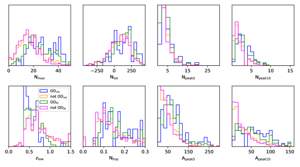
Figure 8: Normalized histograms of our eight introduced selection criteria using the subtracted photo-$z$ distributions. We distinguish between lens candidates visually identified to be in an overdensity (blue) or through the galaxy cluster catalogs (green), compared to those not in an overdensity (orange and magenta, respectively).

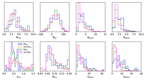
Figure 9: Normalized histograms of our eight introduced selection criteria using the normalized photo-$z$ distributions (which are the subtracted histograms in Fig. 7, normalized by the standard deviation of the 10 000 random sightlines’ histograms). We distinguish between lens candidates visually identified to be in an overdensity (blue) or through the galaxy cluster catalogs (green), compared to those not in an overdensity (orange and magenta, respectively).

Since the distribution of objects in a random field is not flat with respect to redshift, we also test our selection criteria using subtracted photo-$z$ histograms. This means, we create the photo-$z$ histograms for 10 000 random positions in the HSC footprint using our compiled photo-$z$ catalog, and compute the median and the standard deviation per redshift bin. To obtain better statistics at these random positions, we consider here a bin width of 0.06. We now subtract the median histogram from that of all our lens candidates, and apply our criteria to the remaining distribution. As an alternative, we test also normalized histograms defined as the subtracted histograms divided by the standard deviation obtained from the 10 000 histograms at random positions. We show the obtained distribution of our eight selection criteria in Fig. 8 and Fig. 9, respectively. A compilation of possible cuts using the subtracted histograms are listed in Table 4. According to the F1 criterion, the selection on the original histograms performs better. This might be because of the relatively large considered area of $200\arcsec\times 200\arcsec$, centered at the lens candidate, consequently including multiple foreground or background galaxies, such that, although we subtract the median of 10 000 random positions, compact galaxy groups do not obtain a prominent excess in the photo-$z$ distribution of their surrounding objects.

4.4 Final cluster selection

By comparing different cuts on our eight introduced criteria, and taking into account the completeness and purity of the selection through the F1 criterion, we favor No. 46 in Table 3. This gives a completeness rate on the visually identified systems of 58/84 $\sim$ 70%, while 87/174 =50% are listed in the considered galaxy cluster catalogs. We remind that we flagged all overdensities during our visual inspection, including possible group-scale lenses and possible overdense fields not necessarily with most systems at the similar redshift. On the other hand, since the primary focus was the lens grading, the sample cannot be considered as complete. This is already shown through the literature, where we find 174 lens candidates less than 100″ away from a known galaxy cluster, although it is expected that the most distant matches might be missed as we inspected only $80\arcsec\times 80\arcsec$ cutouts centered at the lens candidate. Therefore, it is understandable that we identify some candidates with our photo-$z$ selection that were missed either during the visual inspection or by the galaxy cluster catalogs, which are also not complete. In contrast, the photo-$z$ selection misses some candidates given their distance to the galaxy cluster or due to missing photo-$z$ measurements around the lens candidate. For instance, this is the case for HSC J2329-0120, a grade-B lens candidates visually identified as cluster lens and listed in the galaxy cluster catalog from Wen & Han (2021), as well as the SuGOHI group- and cluster-scale lens sample. While the image stamps analyzed by the network are perfectly fine in all three bands, the $g$ and $r$ bands show $\sim 14\arcsec$ to the north a $\leavevmode\nobreak\ 19\arcsec$ broad stripe without observations. Consequently, in that area no photometric redshifts are available, resulting in a lower number of galaxies in the field. It thus did not pass with a value of 395, our restriction on $N_{\text{tot}}$, while fulfilling the other criteria. These aspects help explain the missing lens candidates identified as lens clusters with other techniques. On the other hand, we obtain with selection No. 46 less than 15% contamination, i.e. lens candidates not identified as galaxy cluster that passes our photo-$z$ criteria.

In total, we have 58 visually identified lens clusters that pass our criteria on the photo-$z$ limits, which include 22 known systems from the SuGOHI group- and cluster-lens catalogs. From these 58 lens cluster candidates, only 15 are not listed in the galaxy cluster catalogs, highlighting the efficiency of the visual inspection in combination with our photo-$z$ criteria. This implies that we identified 43 lens candidates that are (1) listed in the galaxy cluster catalogs, (2) visually identified as clusters and (3) passing photo-$z$ criteria while not being reported in the SuGOHI group- and cluster-scale sample. While these are the most secure newly identified cluster-lens candidates, we consider all lens candidates that pass one of these three criteria as a lens candidate in a significantly overdense environment, resulting in a total of 237/546 systems. For comparison, 136 of 546 lens candidates and 879 random fields from our 10 000 comparison sample, respectively, are passing our photo-$z$ criteria. This shows once more that lenses are on average more often in an overdense environment than random galaxies, and is thus in agreement with e.g., Wells et al. (2024).

5 Conclusion and Discussion

We expanded our systematic search of galaxy-scale lenses by doubling our considered candidates to $\sim$ 135 million objects observed in the HSC Wide survey. We exploit the well tested residual neural network presented by C21, and obtain 11 816 network candidates from the new sample. To identify the most probable lens candidates and reject false positives, we carry out a multi-stage visual inspection with eight individual graders. This ensures stable average grades while limiting the workload though pre-selection with fewer graders. We discuss the procedure in detail, and elaborate recommendations for further visual inspections particularly on large samples such as those expected from the Euclid and Rubin LSST surveys. The proposed strategy is as follows:

• Calibration round: every grader inspect the same small sample which will be then discussed to agree on the grading criteria. This is particularly crucial for new data sets or new grading teams.

• Given the high number of lens search projects carried out, we propose to exclude all previously classified network candidates (i.e., candidates classified as lenses and non-lenses) to lower the number of systems that need inspection, unless the detection algorithm (e.g., modelling rather than CNNs) or data set (e.g., high resolution images from Euclid) has changed notably.

• To reject a significant fraction of false positives, we propose a first inspection by a single person. The goal of this binary classification is to reject only the most obvious interlopers to lower the amount of systems that need to be inspected in the following steps, while keeping any system that require a closer look or system that may gain from a second opinion. In our case, this removed $\sim 90\%$ of the network candidates, mostly images with, e.g., artefacts, or bright saturated stars that were not included in the training data.

• A group of $\sim 4$ individuals inspect the remaining network candidates, providing grades between 0 and 3, and any additional classification flag included (e.g., indicating an offset of the lens, a cluster environment, a possible lensed quasar).

• To further increase the grades per interesting object but lowering the amount of human time, we propose to only collect additional grades for objects with average grade above 1, to finally average over at least seven grades per relevant object. While the threshold for interesting objects is $G\geq 1.5$, we propose here a slightly lower threshold to allow for potential upgrading of candidates after acquiring more grades and to not exclude possible outliers in the grades.

• Finally, a re-classification of systems with high-dispersion among the provided grades.

Following a similar approach, which is described in Sec. 3, we present 24 grade A lens candidates (average grade $G\geq 2.5$) and 138 grade B lens candidates ($2.5>G\geq 1.5$) in Table 1, containing 118 recovered lens candidates already previously identified by complementary algorithms.

While there are a variety of lens search projects carried out, these are nearly always focusing on static galaxy-scale lenses. Given the impact of the lens environment in their analysis and the advantages of cluster-scale lenses for various studies as well as the possibility of exploiting them to study galaxy cluster properties, we present a detailed analysis of their environment. Here, we consider also our previously identified network candidates from C21, enlarging the sample to 546 grade A or B lens candidates. For this, we visually inspect additionally larger image stamps as shown in Fig. 4, and classify their environment.

We further compile and exploit a photo-$z$ catalog obtained from three complementary techniques broadly applied to the HSC Wide survey area, providing finally more than 115 million photo-$z$ values. The presented criteria enable a selection of cluster-lens candidates tested against our visual lens candidate identification and known galaxy clusters from the literature.

The proposed environment analysis paves the way to efficiently exploit larger samples of lens candidates in the upcoming era of wide-field imaging surveys, from which we expect around 100 000 lenses, and which will provide large and accurate photo-$z$ catalogs, as well as a novel technique to identify new lensing clusters.

Appendix A Overview of grade-B lens candidates

In this appendix, we show in Fig. 6 re-centered color-image stamps of our grade B candidates, in analogy to Fig. 3. The image stamps are 12″ on a side and we display the corresponding HSC name in the bottom of each panel, appearing white if discovered for the first time, and light blue if the candidate was previously classified as a grade C candidate. Names in green indicate re-discoveries with comparable grade. In the top we provide the network score $p$ and the average grade $G$. Fully new discoveries are further highlighted with orange frames.

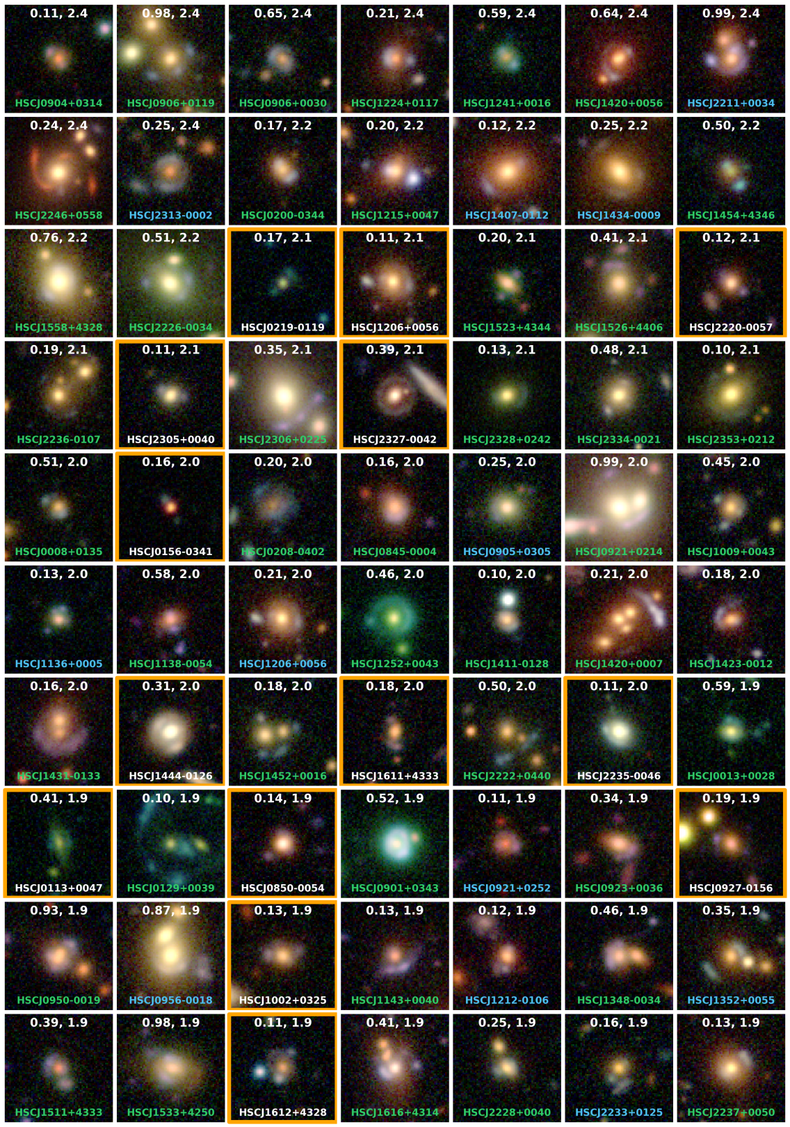
Figure 6: Re-centered color-image stamps of identified grade-B lens candidates. Same format as Fig.3.

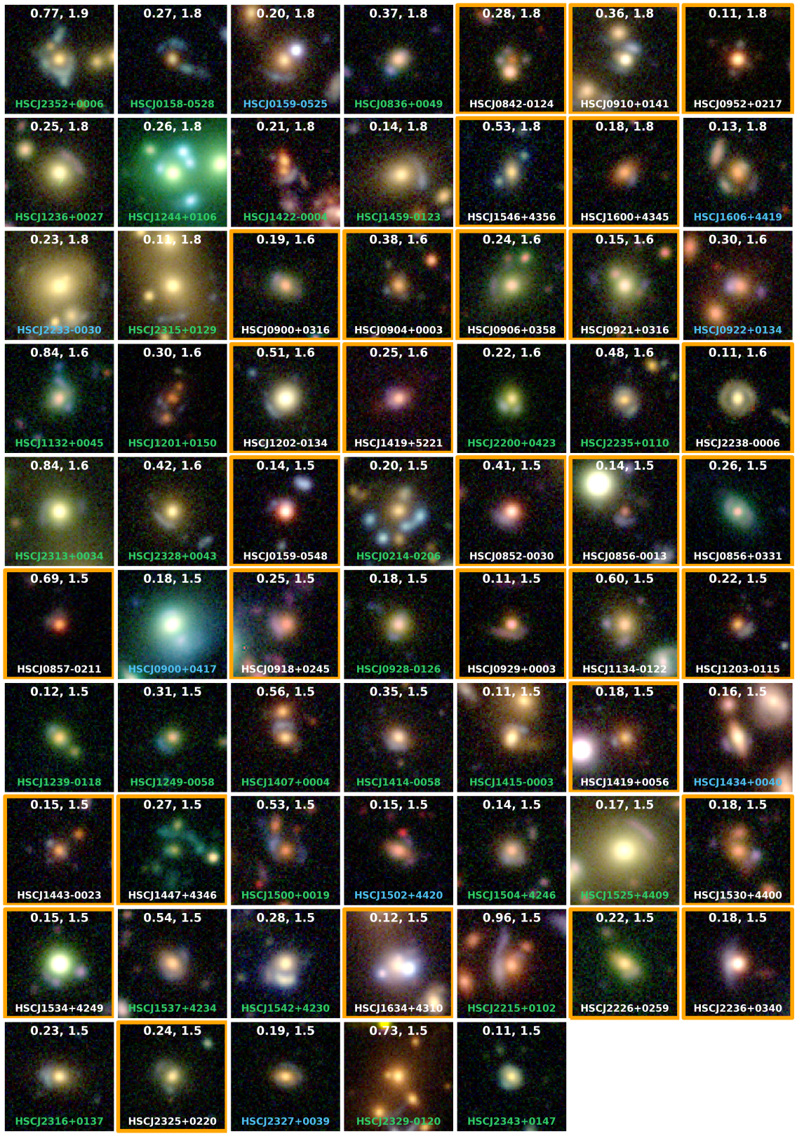
Fig. 6 continued: Re-centered color-image stamps of identified grade-B lens candidates.

Appendix B Further details of lens candidates in overdensities

In this appendix, we provide further details of our lens cluster selection regarding their environment. In detail, Table 4 gives, in analogy to Table 3, the performance of photo-$z$ cuts on the subtracted photo-$z$ histograms, and shows that No. 43 lists the best criteria limits according to the F1${}_{\text{tot}}$ value. We note that this selection is outperformed by No. 46 presented in Sect. 4.3 using the original histograms, instead of the subtracted ones.

In Fig. 7 we show the photo-$z$ histograms of two lens candidates as example, one visually identified to be in an overdense environment (HSC J0214-0206, red) and one not (HSC J0014+0041, blue). In detail, we show the original histograms (top panel), the subtracted histograms (middle panel), and the normalized histograms (bottom panel). The eight selection criteria, introduced in Sect. 4.3, are marked for visualization. For instance, HSC J0214-0206 has with the original histogram (top panel) a value for N${}_{\text{peak}}$ of 26 (horizontal dashed brown line) at $z_{\text{low}}=0.62$ (vertical solid brown line). The sum of the red histogram results in N${}_{\text{tot}}=810$, and consequently N${}_{\text{frac}}=26/810\sim 0.032$. In addition, this histogram shows N${}_{\text{peak5}}=26$ and N${}_{\text{peak10}}=11$ neighbouring redshift bins around $z_{\text{low}}$ that exceeds 5 and 10 (horizontal solid brown line). The sums of objects in these redshift bins are 336 and 189, respectively, denoted as A${}_{\text{peak5}}$ and A${}_{\text{peak10}}$, that are shaded in light and solid red. Following the same style, we also indicate the values of the criteria for the other histograms.

Furthermore, Fig. 8 visualizes the introduced criteria using the subtracted histograms, while Fig. 9 shows them extracted from the normalized histograms. Finally, we show in Fig. 10 $80\arcsec\times 80\arcsec$ image stamps of the remaining grade A and B lens candidates located in an overdense environment based on our visual inspection. This is the continuation of Fig. 4.

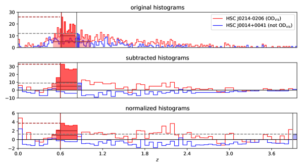
Figure 7: Redshift histograms of two lens candidates as example, one visually identified to be in an overdense environment (HSC J0214-0206, red) and one not (HSC J0014+0041, blue). We show the original histograms (top panel), the histograms where the median distribution of 10 000 random sightlines are subtracted from the original (middle panel), and the normalized histograms (bottom panel) where the subtracted histograms are normalized by the standard deviation of the 10 000 sightlines. Our defined criteria, introduced in Sect. 4.3, are indicated with brown (OD${}_{\text{vis}}$) and gray (not OD${}_{\text{vis}}$) lines. In detail, the vertical solid line indicates $z_{\text{low}}$, the lower bound of the tallest redshift bin of the histogram. The height of this bin, denoted as $N_{\text{max}}$, is marked by the dashed horizontal line. The lengths of the horizontal solid lines, which are the number of the shaded bins, represent $N_{\text{peak5}}$ and $N_{\text{peak10}}$, while the sum of objects in all the shaded bins corresponds to the value of $A_{\text{peak5}}$ and $A_{\text{peak10}}$. See Appendix B for further details.

Table 4: Comparison of true-positive (TP) and false-positive (FP) rates for different selection criteria using the photometric redshift distributions around the 546 grade A or B lens candidates after subtracting a median distribution from 10 000 random sky positions. We distinguish between lens candidates classified as clusters during visual inspection (see Sect. 4.2) and based on galaxy catalogs (Oguri 2014; Oguri et al. 2018; Wen & Han 2018, 2021). Without photo-$z$ selection (see No. 0 in Table 3), we visually identified 84 lens candidates to be in an overdense environment, while 174 lens candidates are located closer than $100\arcsec$ from a known galaxy cluster.

No.	Criteria									visual insp.		Literature		F1 statistics
	$N_{\text{max}}$	$z_{\text{low}}$	$z_{\text{low}}$	$N_{\text{tot}}$	$N_{\text{frac}}$	$N_{\text{peak5}}$	$A_{\text{peak5}}$	$N_{\text{peak10}}$	$A_{\text{peak10}}$	TP	FP	TP	FP	F1${}_{\text{vis}}$	F1${}_{\text{lit}}$	F1${}_{\text{tot}}$
1	$\geq 11$	$\geq 0.1$	$\leq 1.0$	$\geq 0$	$\geq 0.07$	$\geq 0$	$\geq 0$	$\geq 0$	$\geq 0$	69	240	134	175	0.370	0.555	0.474
2	$\geq 11$	$\geq 0.1$	$\leq 1.0$	$\geq 0$	$\geq 0.10$	$\geq 0$	$\geq 0$	$\geq 0$	$\geq 0$	66	194	118	142	0.407	0.544	0.485
3	$\geq 11$	$\geq 0.1$	$\leq 1.0$	$\geq 0$	$\geq 0.13$	$\geq 0$	$\geq 0$	$\geq 0$	$\geq 0$	53	147	98	101	0.402	0.525	0.474
4	$\geq 11$	$\geq 0.1$	$\leq 1.0$	$\geq 50$	$\geq 0.07$	$\geq 0$	$\geq 0$	$\geq 0$	$\geq 0$	60	222	116	155	0.347	0.521	0.445
5	$\geq 11$	$\geq 0.1$	$\leq 1.0$	$\geq 50$	$\geq 0.10$	$\geq 0$	$\geq 0$	$\geq 0$	$\geq 0$	57	176	100	122	0.384	0.505	0.453
6	$\geq 11$	$\geq 0.1$	$\leq 1.0$	$\geq 50$	$\geq 0.13$	$\geq 0$	$\geq 0$	$\geq 0$	$\geq 0$	44	129	80	81	0.371	0.478	0.434
7	$\geq 11$	$\geq 0.1$	$\leq 0.8$	$\geq 0$	$\geq 0.07$	$\geq 0$	$\geq 0$	$\geq 0$	$\geq 0$	69	196	121	144	0.419	0.551	0.495
8	$\geq 11$	$\geq 0.1$	$\leq 0.8$	$\geq 0$	$\geq 0.10$	$\geq 0$	$\geq 0$	$\geq 0$	$\geq 0$	66	159	106	119	0.457	0.531	0.500
9	$\geq 11$	$\geq 0.1$	$\leq 0.8$	$\geq 0$	$\geq 0.13$	$\geq 0$	$\geq 0$	$\geq 0$	$\geq 0$	53	126	91	87	0.436	0.517	0.484
10	$\geq 11$	$\geq 0.1$	$\leq 0.8$	$\geq 50$	$\geq 0.07$	$\geq 0$	$\geq 0$	$\geq 0$	$\geq 0$	60	181	105	126	0.393	0.519	0.465
11	$\geq 11$	$\geq 0.1$	$\leq 0.8$	$\geq 50$	$\geq 0.10$	$\geq 0$	$\geq 0$	$\geq 0$	$\geq 0$	57	144	90	101	0.430	0.493	0.467
12	$\geq 11$	$\geq 0.1$	$\leq 0.8$	$\geq 50$	$\geq 0.13$	$\geq 0$	$\geq 0$	$\geq 0$	$\geq 0$	44	111	75	69	0.402	0.472	0.443
13	$\geq 16$	$\geq 0.1$	$\leq 1.0$	$\geq 0$	$\geq 0.07$	$\geq 0$	$\geq 0$	$\geq 0$	$\geq 0$	67	187	123	131	0.421	0.575	0.509
14	$\geq 16$	$\geq 0.1$	$\leq 1.0$	$\geq 0$	$\geq 0.10$	$\geq 0$	$\geq 0$	$\geq 0$	$\geq 0$	64	148	107	105	0.464	0.554	0.517
15	$\geq 16$	$\geq 0.1$	$\leq 1.0$	$\geq 0$	$\geq 0.13$	$\geq 0$	$\geq 0$	$\geq 0$	$\geq 0$	51	108	88	71	0.457	0.529	0.500
16	$\geq 16$	$\geq 0.1$	$\leq 1.0$	$\geq 50$	$\geq 0.07$	$\geq 0$	$\geq 0$	$\geq 0$	$\geq 0$	60	177	110	122	0.399	0.542	0.481
17	$\geq 16$	$\geq 0.1$	$\leq 1.0$	$\geq 50$	$\geq 0.10$	$\geq 0$	$\geq 0$	$\geq 0$	$\geq 0$	57	138	94	96	0.440	0.516	0.485
18	$\geq 16$	$\geq 0.1$	$\leq 1.0$	$\geq 50$	$\geq 0.13$	$\geq 0$	$\geq 0$	$\geq 0$	$\geq 0$	44	98	75	62	0.427	0.482	0.460
19	$\geq 16$	$\geq 0.1$	$\leq 0.8$	$\geq 0$	$\geq 0.07$	$\geq 0$	$\geq 0$	$\geq 0$	$\geq 0$	67	151	111	107	0.475	0.566	0.528
20	$\geq 16$	$\geq 0.1$	$\leq 0.8$	$\geq 0$	$\geq 0.10$	$\geq 0$	$\geq 0$	$\geq 0$	$\geq 0$	64	118	96	86	0.520	0.539	0.532
21	$\geq 16$	$\geq 0.1$	$\leq 0.8$	$\geq 0$	$\geq 0.13$	$\geq 0$	$\geq 0$	$\geq 0$	$\geq 0$	51	91	82	60	0.495	0.519	0.510
22	$\geq 16$	$\geq 0.1$	$\leq 0.8$	$\geq 50$	$\geq 0.07$	$\geq 0$	$\geq 0$	$\geq 0$	$\geq 0$	60	143	99	100	0.449	0.531	0.497
23	$\geq 16$	$\geq 0.1$	$\leq 0.8$	$\geq 50$	$\geq 0.10$	$\geq 0$	$\geq 0$	$\geq 0$	$\geq 0$	57	110	84	79	0.494	0.499	0.496
24	$\geq 16$	$\geq 0.1$	$\leq 0.8$	$\geq 50$	$\geq 0.13$	$\geq 0$	$\geq 0$	$\geq 0$	$\geq 0$	44	83	70	53	0.461	0.471	0.467
25	$\geq 11$	$\geq 0.1$	$\leq 0.8$	$\geq 0$	$\geq 0.07$	$\geq 3$	$\geq 20$	$\geq 0$	$\geq 0$	66	151	107	128	0.470	0.523	0.501
26	$\geq 11$	$\geq 0.1$	$\leq 0.8$	$\geq 0$	$\geq 0.07$	$\geq 3$	$\geq 30$	$\geq 0$	$\geq 0$	65	146	106	114	0.473	0.538	0.511
27	$\geq 11$	$\geq 0.1$	$\leq 0.8$	$\geq 50$	$\geq 0.07$	$\geq 0$	$\geq 0$	$\geq 2$	$\geq 24$	61	121	102	90	0.496	0.557	0.533
28	$\geq 11$	$\geq 0.1$	$\leq 0.8$	$\geq 50$	$\geq 0.07$	$\geq 0$	$\geq 0$	$\geq 2$	$\geq 30$	60	114	100	82	0.504	0.562	0.539
29	$\geq 11$	$\geq 0.1$	$\leq 0.8$	$\geq 0$	$\geq 0.10$	$\geq 3$	$\geq 20$	$\geq 0$	$\geq 0$	63	118	93	88	0.514	0.524	0.520
30	$\geq 11$	$\geq 0.1$	$\leq 0.8$	$\geq 0$	$\geq 0.10$	$\geq 3$	$\geq 30$	$\geq 0$	$\geq 0$	62	113	92	83	0.519	0.527	0.524
31	$\geq 11$	$\geq 0.1$	$\leq 0.8$	$\geq 50$	$\geq 0.10$	$\geq 0$	$\geq 0$	$\geq 2$	$\geq 24$	58	88	89	67	0.552	0.539	0.544
32	$\geq 11$	$\geq 0.1$	$\leq 0.8$	$\geq 50$	$\geq 0.10$	$\geq 0$	$\geq 0$	$\geq 2$	$\geq 30$	57	83	87	61	0.559	0.540	0.548
33	$\geq 11$	$\geq 0.1$	$\leq 0.8$	$\geq 0$	$\geq 0.07$	$\geq 3$	$\geq 35$	$\geq 0$	$\geq 0$	65	133	104	97	0.496	0.555	0.531
34	$\geq 11$	$\geq 0.1$	$\leq 0.8$	$\geq 0$	$\geq 0.07$	$\geq 3$	$\geq 40$	$\geq 0$	$\geq 0$	64	123	102	87	0.510	0.562	0.541
35	$\geq 11$	$\geq 0.1$	$\leq 0.8$	$\geq 50$	$\geq 0.07$	$\geq 2$	$\geq 20$	$\geq 0$	$\geq 24$	58	128	97	89	0.464	0.539	0.508
36	$\geq 11$	$\geq 0.1$	$\leq 0.8$	$\geq 50$	$\geq 0.07$	$\geq 2$	$\geq 20$	$\geq 0$	$\geq 30$	58	115	93	80	0.489	0.536	0.517
37	$\geq 11$	$\geq 0.1$	$\leq 0.8$	$\geq 0$	$\geq 0.10$	$\geq 3$	$\geq 35$	$\geq 0$	$\geq 0$	62	100	90	75	0.549	0.531	0.538
38	$\geq 11$	$\geq 0.1$	$\leq 0.8$	$\geq 0$	$\geq 0.10$	$\geq 3$	$\geq 40$	$\geq 0$	$\geq 0$	61	91	88	66	0.565	0.537	0.548
39	$\geq 11$	$\geq 0.1$	$\leq 0.8$	$\geq 50$	$\geq 0.10$	$\geq 2$	$\geq 20$	$\geq 0$	$\geq 24$	55	94	84	65	0.516	0.520	0.519
40	$\geq 11$	$\geq 0.1$	$\leq 0.8$	$\geq 50$	$\geq 0.10$	$\geq 2$	$\geq 20$	$\geq 0$	$\geq 30$	55	84	80	59	0.542	0.511	0.523
41	$\geq 15$	$\geq 0.1$	$\leq 0.8$	$\geq 50$	$\geq 0.10$	$\geq 0$	$\geq 0$	$\geq 2$	$\geq 24$	57	83	87	62	0.559	0.539	0.546
42	$\geq 15$	$\geq 0.1$	$\leq 0.8$	$\geq 50$	$\geq 0.10$	$\geq 0$	$\geq 0$	$\geq 2$	$\geq 30$	57	80	86	59	0.567	0.539	0.550
43	$\geq 15$	$\geq 0.1$	$\leq 0.8$	$\geq 50$	$\geq 0.10$	$\geq 0$	$\geq 35$	$\geq 2$	$\geq 24$	57	80	86	58	0.567	0.541	0.551
44	$\geq 15$	$\geq 0.1$	$\leq 0.8$	$\geq 50$	$\geq 0.10$	$\geq 0$	$\geq 45$	$\geq 2$	$\geq 24$	56	74	82	52	0.577	0.532	0.550
45	$\geq 15$	$\geq 0.1$	$\leq 0.8$	$\geq 50$	$\geq 0.10$	$\geq 0$	$\geq 35$	$\geq 2$	$\geq 30$	57	78	85	57	0.573	0.538	0.551
46	$\geq 15$	$\geq 0.1$	$\leq 0.8$	$\geq 50$	$\geq 0.10$	$\geq 0$	$\geq 45$	$\geq 2$	$\geq 30$	56	73	81	52	0.580	0.528	0.548

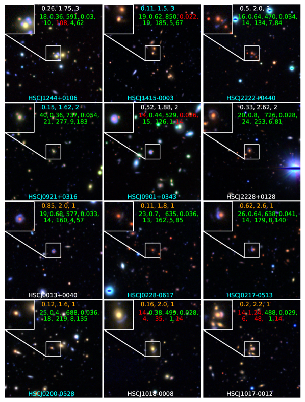
Figure 10: New grade A and B group- or cluster lens candidates based on visual inspection. Continuation of Fig. 4.

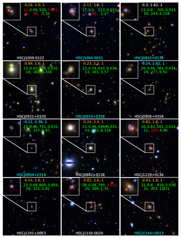
Fig. 10 continued: New grade A and B group- or cluster lens candidates based on visual inspection.

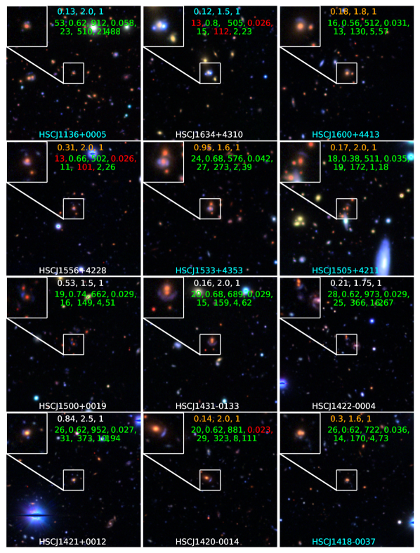
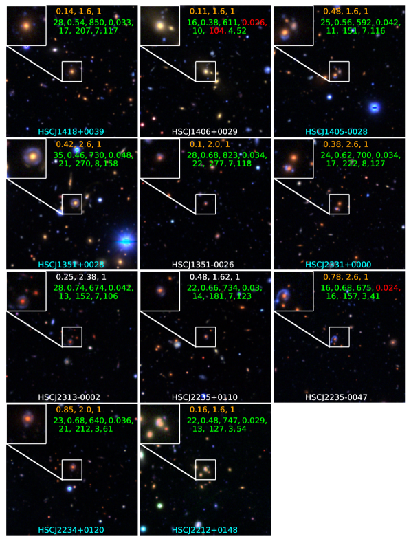
Fig. 10 continued: New grade A and B group- or cluster lens candidates based on visual inspection.

Fig. 10 continued: New grade A and B group- or cluster lens candidates based on visual inspection.