Dipole-dipole interactions mediated by a photonic flat band
Abstract
Flat bands (FBs) are energy bands with zero group velocity, which in electronic systems were shown to favor strongly correlated phenomena. Indeed, a FB can be spanned with a basis of strictly localized states, the so called compact localized states (CLSs), which are yet generally non-orthogonal. Here, we study emergent dipole-dipole interactions between emitters dispersively coupled to the photonic analogue of a FB, a setup within reach in state-of the-art experimental platforms. We show that the strength of such photon-mediated interactions decays exponentially with distance with a characteristic localization length which, unlike typical behaviours with standard bands, saturates to a finite value as the emitter’s energy approaches the FB. Remarkably, we find that the localization length grows with the overlap between CLSs according to an analytically-derived universal scaling law valid for a large class of FBs both in 1D and 2D. Using giant atoms (non-local atom-field coupling) allows to tailor interaction potentials having the same shape of a CLS or a superposition of a few of these.
I Introduction
The coherent interaction between quantum emitters and engineered low-dimensional photonic environments is a hot research area of modern quantum optics, especially in the emerging framework of waveguide QED [1, 2, 3, 4, 5]. A core motivation is unveiling qualitatively new paradigms of atom-photon interaction, well beyond those occurring in standard electromagnetic environments (like free space or low-loss cavities). These can potentially be exploited to implement cutting-edge quantum information processing tasks or to favor observation of new quantum many-body phenomena. This relies on the fact that photonic baths with tailored properties and dimensionality, e.g. photonic versions of electronic tight-binding models, can today be implemented in a variety of experimental scenarios. This includes photonic crystals in the optical domain [6, 7, 8, 9], superconducting circuits in the microwaves [10, 11, 12, 13] and matter-wave emulators [14, 15], allowing the study even of lattices with non-trivial properties such as non-trivial topological phases (even in 2D) [16, 17] or able to emulate curved spaces [18].
A key phenomenon to appreciate the effect of an engineered photonic bath are photon-mediated dispersive interactions. For instance, while a high-finesse cavity can mediate an effective all-to-all interaction between atoms in the dispersive regime [19, 20], replacing the cavity with an engineered lattice of coupled cavities can result in interactions with a non-trivial shape of the interatomic potential when the atoms are tuned in a photonic bandgap [21, 22]. The resulting interaction range can be controlled via modulating the detuning from the band edge, which has been experimentally confirmed in circuit QED [23, 16, 13, 24] and predicted to be a resource for efficient quantum simulations [25, 26, 27] and implementation of hybrid quantum-classical algorithms [28]. Such effective coherent interactions between atoms can be understood as being mediated by atom-photon bound states (BSs) formed by a single quantum emitter [29, 30, 31, 32, 33, 11, 34, 35, 36, 15, 37, 38], whose corresponding photonic wavefunction (typically exponentially localized around the atom) in fact shapes the spatial profile of the effective interatomic potential [21, 39, 40].
Remarkably, due to destructive interference mechanisms, some lattices can host a special type of bands having in fact the same spectrum as a (one-mode) cavity. Such a band is called flat band (FB) in that its dispersion law is flat. Accordingly, a FB has zero width so that its spectrum features only one frequency just like a perfect cavity mode. Such kind of bands are well-known to show up in certain natural and artificial lattice structures [41, 42], a prominent example occurring in the celebrated quantum Hall effect [43]. FBs are currently investigated in condensed matter and photonics [44] because, due to their macroscopically large degeneracy and effective quenching of kinetic energy, they can favor emergence of many-body effects, highly-correlated phases of condensed matter [45] and non-linearity [46]. Moreover, FBs are extremely sensitive to disorder [47]. Typically, a FB arises when the lattice structure is such that, for each unit cell, one can construct a compact stationary state (i.e. strictly localized on a few sites), which exactly decouples from the rest of the lattice by destructive interference. As a hallmark, these states, called Compact Localised States (CLSs) [48, 49, 50] in most cases are non-orthogonal and can be used to construct a basis of localized states spanning the FB space that is alternative to the canonical basis of Bloch states (these being in contrast orthogonal and unbound).
Given the above framework, here we tackle the question as to what kind of photon-mediated interactions are expected when atoms are dispersively coupled to a photonic FB, and in particular whether they are like those in the vicinity of a standard band (i.e. with finite width) or instead like typical ones in cavity QED. The question is non-trivial as a FB has the same dimensionality of a standard band but, in contrast, zero bandwidth. On the other hand, a FB has a spectrum comprising only one frequency like a one-mode cavity but, in contrast, contains a thermodynamically large number of modes.
With these motivations, this paper presents a general study of atom-photon interactions in the presence of photonic FBs 111Atoms coupled to photonic FBs in specific models appeared in recent studies [70, 71, 72]., by focusing in particular on photon-mediated interactions whose associated potential shape is inherited (as for standard bands) from the shape of atom-photon BSs. In contrast to the edge of a standard band, it turns out that in the vicinity of a FB the shape of the BS is insensitive to the detuning, while the interaction range of photon-mediated interactions generally remains finite even when the atom energetically approaches the FB.
Importantly, we connect the atom-photon BS to the form of the photonic CLSs characteristic of the considered band by demonstrating that the overlap between CLSs provides the mechanism which enables atoms in different cells to mutually interact. We derive an analytical and exact general relationship between the BS localization length and the non-orthogonality of CLSs valid for a large class of 1D and 2D lattices.
This work is organized as follows. In Section II, we introduce the model and notation and review some basic concepts concerning atom-photon bound states and photon-mediated interactions. In Section III, we present a case study illustrating some peculiar features of BSs in the presence of FBs and highlighting differences from standard bands. In Section IV, we review the concept of Compact Localised States and introduce some 1D models used in this paper. General properties of bound states seeded by a FB are derived and discussed in Section V, while the case of a giant atom coupled to a FB system and the ensuing photon-mediated interactions is addressed in Section VII. Finally, in Section VIII we draw our conclusions.
II Setup and review of photon-mediated interactions
Here, we introduce the general formalism we will work with and review some basic notions and important examples of photon-mediated interactions. We start from atom-photon BSs, which are necessary in order to appreciate the physics in the presence of FBs to be presented later.
II.1 General model
We consider a quantum emitter modeled as a two-level system whose pseudo-spin ladder operator is , with and being respectively the ground and excited states, whose energy difference is . The atom is locally coupled under the rotating-wave approximation to a photonic bath modeled as a set of single-mode coupled cavities or resonators each labeled by index (which is generally intended as a set of indexes). Accordingly, the total Hamiltonian reads
| (1) |
where labels the cavity which the emitter is coupled to with strength . The free Hamiltonian of the photonic bath reads
| (2) |
where is the bare frequency of the th cavity, () the associated creation (destruction) bosonic ladder operator while denotes the photon hopping rate between cavities and . The Fock state where cavity has one photon (with all the remaining ones having zero photons) will be denoted as , where is the vacuum state of the field.
While many properties discussed in this paper require solely that the bath possesses a FB, which can happen even if the photonic bath is not translationally-invariant, all of the examples that we will discuss concern photonic lattices. In these cases, is a -dimensional lattice so that index in the above equations should be intended as the pair of indexes , where stands for integers labelling a primitive unit cells around the Bravais lattce vector , each while labels the sublattices. Notice that in this work we will express all length in units of the lattice constant. The normal frequencies of (in the thermodynamic limit) comprise a series of bands, labeled by index and with corresponding dispersion law , where the -dimensional wave vector lies in the first Brillouin zone (to make notation lighter, we will write in place of whenever possible). Accordingly, the bath Hamiltonian can be written in diagonal form as
| (3) |
where and are ladder operators associated with the th band.
Throughout this work, we will focus on the single-excitation sector, i.e. the subspace spanned by the set (with running over all cavities). For the sake of simplicity, we will adopt a lighter notation in what follows and replace
Hence, from now on will be the state where the excitation lies on the atom and the field has no photons, while is the state where the atom in the ground state and a single photon at cavity has one photon (with each of the remaining cavities in the vacuum state). In particular, is the state where a single photon lies at cavity (the one directly coupled to the emitter).
II.2 Atom-photon bound states
Within the single-excitation sector, an atom-photon bound state (BS) is a normalized dressed state such that , where is a real solution of the pole equation
while the wavefunction (up to a normalization factor) reads [29]
| with | (4) |
Here, is the bath resolvent or Green’s function in the single-excitation subspace [29], whose general definition is [cf. Eq. (3)]
| (5) |
When is not a lattice, index is just replaced by the index(es) labelling the eigenmodes of the field.
Typically, a BS occurs when the atom is coupled off-resonantly to (as in all examples to be discussed in this paper where will be tuned within a bandgap of bath ). In this case, to leading order in the coupling strength we have
| (6) |
Wavefunction (to be normalized) describes a single photon localized around the atom’s location .
The simplest, and in some respects trivial, example of an atom-photon BS occurs in a single-mode cavity, i.e. when . In this case, the bath Green’s function simply reads so that the BS reduces to 222This is one of the two dressed states in the single-excitation sector, specifically the one with a dominant atomic component. The other state instead has energy and is mostly photonic..
Another paradigmatic instance of BS occurs when is a 1D lattice of coupled cavities described by the Hamiltonian with . The energy spectrum (in the thermodynamic limit) consists of a single band in the interval with dispersion law . The corresponding Green’s function (for out of the band) reads [53, 54]
| (7) |
where the last equality holds in the thermodynamical limit () and for (so that the atomic frequency lies above the upper band edge) and . Here, we see that the BS is exponentially localized with
| (8) |
Thus, the photon is exponentially localized around the atom over a region of characteristic length (localization length). Remarkably, this scales as , entailing that, as the atomic frequency approaches the band edge (i.e. for ), the BS gets more and more delocalized. Later on, we will see that in the presence of a FB a very different behavior occurs with the BS localization length saturating to a constant value as .
II.3 Effective Hamiltonian with many emitters
In the presence of many identical emitters, each indexed by , the Hamiltonian (1) is naturally generalized as
| (9) |
with labeling the cavity which the th atom is coupled to.
When lies within a photonic bandgap and is in the vacuum state, the field degrees of freedom can be adiabatically eliminated and the dynamics of the emitters is fully described by the effective many-body Hamiltonian [21, 22, 40]
| (10) |
where
| (11) |
Here, is the BS seeded by the th atom, whose expression is analogous to Eq. (6) with in place of . Thus, when atoms are dispersively coupled to the bath , they undergo a coherent mutual interaction described by the effective interatomic potential . Significantly, Eq. (11) shows that the interaction strength between a pair of atoms is simply proportional to the BS seeded by one emitter (as if this were alone) on the cavity where the other emitter sits in. Thus, the BS wavefunction of a single emitter in fact embodies the spatial shape of the photon-mediated interaction potential in the presence of many emitters in the dispersive regime.
Based on the discussion in Section II.2, for a set of atoms all coupled to a single cavity we get irrespective of and , meaning that the emitters undergo an all-to-all interaction.
Instead, owing to the exponential localization of BS (8), a set of atoms dispersively coupled to a homogeneous cavity array (see Section II.2) undergo an effective short-range interaction described by
| (12) |
where the BS localization length [see Eq. (8)] can now be seen as the characteristic interaction range depending on .
III Bound state near a photonic flat band: case study

A major difference between the two paradigmatic baths considered so far, i.e. a cavity versus a coupled-cavity array, is that the latter can host propagating photons whose speed is proportional to the slope of the dispersion law . Notice that the presence of a non-trivial dispersion law is essential for the occurrence of photon-mediated interactions with finite and -dependent interaction range [cf. Eqs. (8) and (12)].
In the remainder of this paper, we will deal with dispersive physics near a flat band (FB). A FB is a special photonic band whose dispersion law is -independent, i.e.
| (13) |
Thus, unlike a standard band, a FB has zero bandwidth, a feature shared with a (perfect) cavity. Differently from a cavity and analogously to a standard band, however, the FB energy has a thermodynamically large degeneracy (matching the number of lattice cells ) 333If bath is not a lattice, a FB occurs when there exists a normal frequency with a thermodynamically large degeneracy. An instance of such a situation are certain kinds of hyperbolic systems, where there exists a FB gapped from the rest of the energy spectrum [18]..
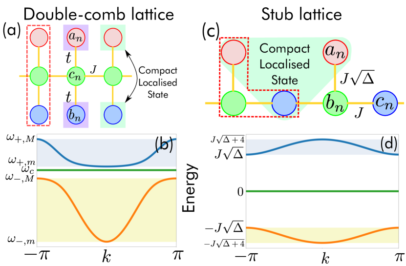
In order to introduce some typical properties of photon-mediated interactions around a FB, in this section we will consider the case study of the 1D sawtooth photonic lattice in 1(a) [56, 57], arguably the simplest yet non-trivial system where a FB shows up. This is a bipartite lattice, where the th cell consists of a pair of cavities labeled and . Each cavity is coupled to its nearest neighbours with photon hopping rate and with rate to cavities and . 444Strictly speaking, this is a special case of the sawtooth lattice in which the ratio of the two hopping rates is constrained so as to ensure the emergence of a FB.. All cavities have the same bare frequency which we set to zero. The two bands of have dispersion laws (see Appendix A)
| (14) |
As shown in 1(b), the band labeled by subscript is a standard dispersive band of width 4, below which a FB of energy stands out (the energy separation of this from the edge of band is ).
We now discuss the atom-photon BS formed by an emitter dispersively coupled to the 1D sawtooth lattice in the two different regimes where the effect of either the FB or the dispersive band is negligible. We start by tuning very far from the FB (so that this can be fully neglected) but relatively near the lower edge of the dispersive band so as to fulfill with and respectively the detuning from the lower edge of band and from the FB [see 1(b)]. The spatial profile of the BS photonic wavefunction is plotted in 1(c)-(e) for decreasing values of . Similarly to Eq. (8) (homogeneous array), the BS is exponentially localized around the atom with a localization length which diverges as .
We next consider the regime [see 1(b)] in a way that the atom is significantly (although dispersively) coupled only to the FB with the contribution of the dispersive band now negligible. As shown in 1(f)-(h), instead of diverging, the BS localization length now saturates to a finite value as . Correspondingly, the BS wavefunction no longer changes when is small enough, which shows that this asymptotic BS is insensitive to the atom frequency.
The simple instance just discussed suggests that atom-photon BSs in the vicinity of a photonic FB, along with the ensued photon-mediated interactions, have a quite different nature compared to standard photonic bands. While the fact that the BS remains localized is somewhat reminiscent of the behavior in a standard one-mode cavity, it is natural to wonder what the BS localization length depends on. It will turn out that this depends on the way in which the emitter is coupled to the lattice as well as some intrinsic properties of the FB, in particular the orthogonality of the so called Compact Localized States (CLSs), a key concept in FB theory. For this reason, the next section is fully devoted to a review of CLSs, whose main properties will be illustrated through variegated examples. This will provide us with the necessary theoretical basis to formulate general properties of BSs in Section V, including more general types of FBs (e.g. occurring in 2D lattices).
IV Compact localized states
As for any band, the eigenspace made up by all photonic states where a single photon occupies a given FB can be naturally spanned by the Bloch stationary states with , where runs over the first Brillouin zone (we omit the band index in to make notation lighter).
Accordingly, the projector onto the FB eigenspace in the Bloch states basis reads
| (15) |
By definition, when is applied to a generic single photon state it returns its projection onto the FB eigenspace. Notice that, being translationally invariant (see Bloch theorem [59]), each basis state is necessarily unbound, i.e. its wavefunction has support on the entire lattice. Yet, since photons in a FB have zero group velocity [cf. Eq. (13)], it is natural to expect the FB eigenspace to admit an alternative basis of localized (i.e. bound) states , one for each unit cell indexed by (when is a lattice). Such a basis indeed exists and its elements are called Compact Localised States (CLSs) [48] (an exception occurs when the FB touches a dispersive band, a pathological case that we will address later on). Note that a CLS is compact in the sense that, typically, it is strictly localized only on a finite, usually small, number of neighbouring unit cells. There exists a general way to express CLSs in the basis of Bloch states for a -dimensional latttice, which reads [48]
| (16) |
with the number of cells and where is a suitable function (recall that is a Bravais lattice identifying a unit cell).
The idea behind CLSs is somewhat similar to standard Wannier states [60] in that a CLS can be expressed as a suitable superposition of unbound Bloch states that yields a state localized around a lattice cell. Unlike a Wannier state, however, a CLS is itself an eigenstate of the bath Hamiltonian, i.e. , since the Bloch states entering the expansion all have the same energy (reflecting the high FB degeneracy).
IV.1 Class
Note that, while there is a one-to-one correspondence between CLSs and unit cells, a CLS is generally spread over cells, where the positive integer is the so called class of the CLS set [61]. In the special case , each is entirely localized within the th cell so that the CLSs do not overlap in space and are thus orthogonal, i.e. (an instance is the double-comb lattice of 2). For , instead, CLSs necessarily overlap in space with one another, which remarkably causes them to be generally non-orthogonal. It is easy to convince oneself that for a 1D (generally multipartite) lattice CLSs of class are such that each CLS overlaps only its two nearest-neighbour CLSs, being orthogonal to the all the remaining ones (an instance is the sawtooth lattice of 1 which we will discuss shortly). For 2D lattices, it is easier to think of class as a 2D vector of integer components, describing how many cells the CLS is spread over along either direction. For instance, if the CLS will overlap only its nearest-neighbours along each direction (an instance being the checkerboard lattice of 5 to be discussed later on).
Notice that, owing to the degeneracy of the FB energy , the set of CLSs spanning the FB eigenspace for a given lattice is not unique. We call minimal the set of CLSs having the lowest class . In the remainder, we will only consider minimal CLSs.
IV.2 Instances of CLSs in 1D lattices
In order to make the reader familiarize with CLSs and their properties (especially non-orthogonality), we present next some examples of lattices exhibiting FBs [see 2 and 3]. In this section, we will only discuss 1D models, meaning that here the cell index is an integer and the wavevector a real number (see Appendix A for more details on those models).
IV.2.1 Double-comb lattice
The double-comb lattice is a tripartite lattice, which comprises three sublattices and [see 2(a)]. Each cavity of the central sublattice is coupled to the nearest-neighbour cavities with photon hopping rate and with rate to cavities and (upper and lower sublattices, respectively). Cavities and have the same bare frequency , while the one of is set to zero. The spectrum of , which is plotted in a representative case in 2(b), features a FB at energy and two dispersive bands. The occurrence of such FB is easy to predict since the antisymmetric state
| (17) |
clearly decouples from state (hence the rest of the lattice) due to destructive interference and is thereby an eigenstate of the bath Hamiltonian with energy . Evidently, there exists one such state for each cell , explaining the origin of the FB at energy . As each is strictly localized within a unit cell [see 2(a)], states form a set of orthogonal CLSs of class based on the previous definition.
IV.2.2 Sawtooth lattice
We already introduced the sawtooth lattice in Section III and 1. Somewhat similarly to the double-comb lattice, the FB at also arises through destructive interference. Indeed, the superposition
| (18) |
decouples from sites , hence the rest of the lattice. Since we can build up one such state for each cell, the set form a basis spanning the FB eigenspace. Unlike the double-comb lattice, however, it is clear that each state is not localized within a single unit cell and is not orthogonal to the two CLSs [cf. 1(a)]. Indeed, it is easy to verify that
| (19) |
with . Therefore, these CLSs form a non-orthogonal basis of the FB eigenspace and, since each CLS overlaps only nearest-neighbour states, this set is of class .
IV.2.3 Stub lattice
The stub lattice (or 1D Lieb lattice) [56, 62, 63] is the tripartite lattice sketched in 2(c), where each cavity is coupled to cavities with rate and side-coupled to cavity with rate where is a dimensionless parameter. The spectrum of is symmetric around , at which energy a FB arises (). The gap separating the FB from each dispersive band is proportional to [see 2(c)].
Similarly to the previous lattices and CLSs, the origin of the zero-energy FB can be understood by noting that state
| (20) |
decouples from the rest of the chain. Like in the sawtooth lattice, the non-orthogonal set form a CLS of class since Eq. (19) holds also in the present case with
| (21) |
Notice that controls both the overlap between CLSs and the energy gap between the FB and each dispersive band (such a tunability is not possible in the sawtooth model). For we get and zero band gap. For growing , the non-orthogonality parameter gets smaller and smaller [indeed is more and more localized around cavity , cf. (20)] while the gap gets larger and larger.
Note that the stub lattice enjoys chiral symmetry [64] which guarantees a zero-energy FB to exist [65] even in the presence of disorder provided that it does not break chiral symmetry 555This zero-energy FB always exists in lattices with chiral symmetry and an odd number of sublattices (Lieb’s Theorem [65]). This is because chiral energy imposes the energy spectrum to be symmetric around for any . As the total number of energy bands is odd, one of the bands must necessarily be a zero-energy FB..

IV.2.4 1D Kagomè lattice
The 1D Kagomè model sketched in 3(a) is a lattice with five sublattices, representing the 1D version of the popular 2D Kagomè model [67]. In this model each cavity is coupled to its nearest neighbour with rate , except for pairs () and () which are coupled with rate .
This system differs from the previous instances in that there exists a FB (of frequency ) which touches the edge of a dispersive band [see 3(b)].
V Bound states in a FB: general properties
Armed with the notion of CLSs, we are now ready to establish general properties of atom-photon BSs.
V.1 Atom-photon bound state as a superposition of compact localized states
We recall that the BS shape is generally dictated by the field’s bare Green’s function [see Eq. (4)]. As in the examples discussed in Section III, here we consider the regime where the emitter is dispersively coupled to one specific band (not necessarily a FB), which we will call , in such a way that the effects of all the other bands can be neglected. This in particular happens when, as in Section III, there is a finite energy gap between band and all the other bands (no band crossing/touching). Another circumstance where this regime holds (as we will see later on) is when the contribution of band to the density of states (at energies close to ) is dominant compared to that from the other bands.
In such regime, we can approximate the BS wavefunction as [cf. Eqs. (4), (5) and (6)]
| (23) |
(notice that only the contribution of band is retained).
Wavefunction , including its shape and width, will generally depend on the emitter frequency , hence on its detuning from the th band edge. However, if band is a FB, in Eq. (23) we can replace with , which is -independent, and obtain the BS wavefunction (here labels a generic lattice site, even beyond 1D)
| (24) |
where we substituted the projector on the FB eigenspace [see Eq. (15)]. Evidently, the shape and width of the BSs become independent of the detuning of the atom from the FB in agreement with the behaviour emerging from 1(f)-(h). Notice that this independence holds also for an atom dispersively coupled to a standard cavity in which case however the BS is trivial.
Having assessed the independence of the detuning, we next characterize the structure and spatial range of the BS (which will then also be those of photon-mediated interactions, see Section II.3). For this aim, taking advantage of Eq. (16), it is convenient to re-express the FB projector (15) in terms of the CLSs basis as (see Appendix B for details)
| (25) |
with
| (26) |
Notice that the scalar product between two CLSs depends on function as [cf. Eq. (16)]
| (27) |
Remarkably, unlike the Bloch-states expansion of Eq. (15), the decomposition of Eq. (25) in terms of CLSs is non-diagonal. This is a consequence of the CLSs’ non-orthogonality discussed in the previous section. Indeed, for (orthogonal CLSs) we have and hence in a way that Eq. (25) reduces to a standard diagonal expansion in the CLS basis. On the other hand, provided that only nearest-neighbour CLSs are overlapping (as in all the examples of this work), is generally given by
| (28) |
where is the lattice dimension, the th component of wave vector and the overlap between a pair of nearest-neighbour CLSs lying along the th direction. It is clear that since we have .
Finally, plugging Eq. (25) into Eq. (24) yields
| (29) |
with
| (30) |
which expresses the BS wavefunction as a weighted superposition of CLSs where the weight function is defined by Eq. (30) and depends on the cavity to which the emitter is coupled to. In particular, the weight function is proportional to , which is non-zero only if cavity overlaps the CLS . As a consequence, being the CLSs strictly compact, the weight function [cf. Eq. (30)] involves only a finite number of terms.
Expansion (29) is a central result of this work. Notice that for non-overlapping CLSs (class ) we have (since as we saw previously), which entails that in this case the BS just coincides the CLS overlapping the cavity (if any). Hence, for , atoms sitting in different cells will just not interact. This situation is reminescent of cavity QED, where CLSs play the role of non-overlapping cavity modes: atoms in isolated cavities have no way to cross-talk. In this sense, FBs of class show a cavity-like behaviour. In contrast, for , CLSs do overlap each other in a way that now and thus the BS is a superposition of more than one CLS. We see that the interaction between atoms located in different cells is now possible and this is a consequence of the CLSs’ overlap. This situation is quite different from standard cavity QED. In particular, the CLSs cannot be interpreted as overlapping cavity modes since, if so, these would in fact couple the cavities affecting their spectrum non-trivially (in contrast to the present FB).
In the following, we consider the recurrent case where only nearest-neighbour CLSs overlap, which happens for for 1D lattices and for 2D ones (cf. Section IV.1) and show that the BS is exponentially localized by deriving the localization length as an explicit general function of the CLSs’ overlap.
V.2 1D lattices,
In this case, Eq. (28) reduces to , with . Plugging this into Eq. (26) and working out the resulting integral in the thermodynamic limit (), one ends up with (see Appendix C for the proof)
| (31) |
where denotes the sign of while
| (32) |
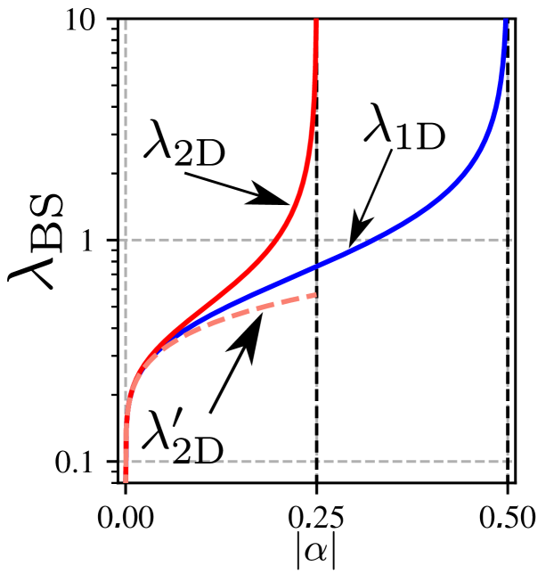
being the inverse function of the hyperbolic secant. Therefore, decays exponentially with with a characteristic length which is a growing function of the non-orthogonality coefficient [see 4(b) showing that vanishes for and diverges for ]. Based on a result derived in Appendix D, we get that the BS has the same exponential shape and localization length as . For instance, in the case of the sawtooth lattice [see Eq. (19)] we have , which replaced in Eq. (31) yields in perfect agreement with the scaling observed in 1(f-h).
V.3 2D lattices,
For a 2D lattice and a square geometry (we focus on this case as all our 2D examples have such structure), Eq. (28) is given by . For the sake of argument, we focus on the isotropic case , (a generalization to is straightforward but expressions get involved). One can then show that (see Appendix C)
| (33) |
where are constants while
| (34) |
( is subject to the constraint ). Thus, in this case the decay results from the superposition of two exponential functions with localization length and , respectively. As in 1D, both localization lengths grow with (see 4(b)]. Differently from 1D, however, when approaches its maximum value 1/4 only diverges while instead saturates to the finite value (for , saturates to the same value while diverges).
This means that in this limiting case the weight function is a single exponential having localization length equal to . In 2D, thereby, photon-mediated interactions are finite-ranged provided that the CLSs have non-zero overlap.
VI Flatband touching a dispersive band
The conclusions developed so far apply to lattices featuring an energetically isolated FB, i.e. separated by a finite gap from all the remaining bands [recall Eq. (24) where only the contribution of the FB is retained]. This rules out in particular those lattices where a FB arises on the edge of a dispersive band. In 1D, such band touching happens for example in the stub lattice for (see Section IV.2.3 and 2) and in the Kagomè model (see Section A.4 and 3). Indeed, it turns out that in either case, an atom dispersively coupled to the FB seeds a BS with features analogous to typical BSs close to the band edge of an isolated dispersive band [e.g. as in 1 (c)-(e)]. This is witnessed by 3(c) for the Kagomè model, which shows that the BS localization length gets larger and larger as the detuning from the FB decreases in contrast to the saturation behavior next to an isolated FB that occurs e.g. in 1 (f)-(h). Notice that in these 1D examples the dispersive band scales quadratically in the vicinity of the FB.
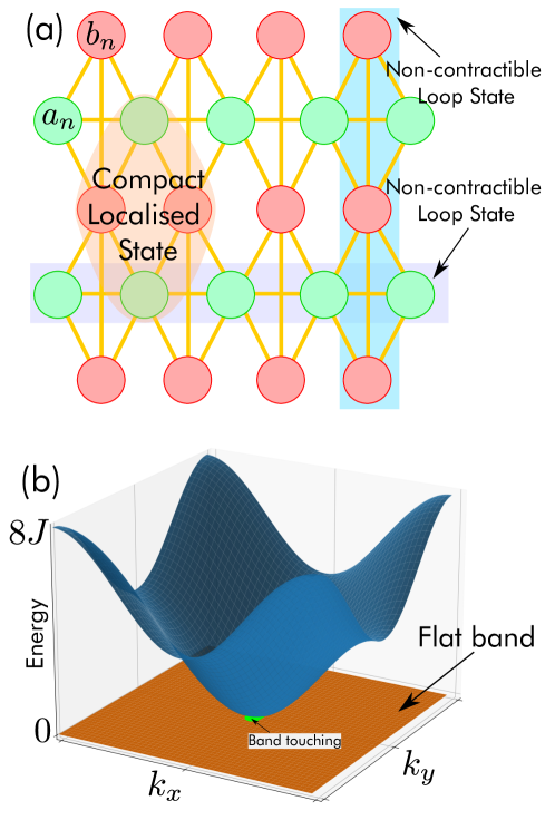
FBs falling on the edge of dispersive bands can also occur in 2D. A paradigmatic instance is the checkerboard lattice in 5(a). This a bipartite lattice where nearest-neighbour cavities of the same sublattice are coupled with hopping rate , while the hopping rate between nearest-neighbour cavities of different sublattices is along one diagonal and along the other diagonal. Each cavity has frequency . The spectrum features a FB and a dispersive band according to [see also 5(b)]
| (35) |
The two bands touch one another at the point (close to this has a parabolic shape). A set of non-orthogonal CLSs, one for each unit cell, is easily identified as [see 5(b)]
| (36) |
where labels unit cells 666Unlike previous examples of overlapping CLSs, the set (36) is not a complete basis of the FB eigenspace, which can be shown to be due to the singular behaviour of the present FB [48]. To get a complete basis, the set (36) must be complemented with a pair of so called non-contractible loop states [see 5(b)]. These two states are yet unbound, hence in the thermodynamic limit we can neglect their contribution to the BS (this arising from the local atom-field interaction).. We are thus in the case with the overlap between nearest-neighbour CLSs being given by .
Now, remarkably, we numerically checked that an atom dispersively coupled to the FB at gives rise to a BS whose features accurately match those predicted in Section V.3 for , meaning that localization length is independent of the detuning and has the finite value [recall the discussion after Eq. (34)]. In other words, we find that the behaviour is identical to that of an energetically isolated FB.
The above case studies can be understood by recalling that a dispersive band that scales quadratically in the vicinity of a band edge gives a contribution to the density of states (DOS) which is finite in 2D while it diverges in 1D (in the latter case a van Hove singularity occurs). In contrast, the DOS of a FB clearly has -like diverging at . It follows that in 2D the dispersive band can be neglected compared to the FB, explaining why in this case the properties of the BS match those predicted for an isolated FB in Section V.3. In 1D, instead, the contribution of the dispersive band can no longer be neglected, explaining why e.g. in the Kagomè lattice the BS behaviour is different from the one in Section V.2.
VII Giant atoms coupled to a photonic flat band
In recent years, it has become experimentally possible fabricating so called giant atoms [69], i.e. quantum emitters which are coupled non-locally to the field through a discrete set of coupling points (where a standard atom is retrieved in the special case of only one coupling point). For a giant atom with coupling points the total Hamiltonian (1) is generalized as
| (37) |
where (coupling point) labels the cavity to which the giant atom is coupled to and the corresponding (generally complex) coupling strength. It is convenient to define the field ladder operator [40]
| (38) |
where, due to , fulfills . With this definition, (37) can be arranged formally as the Hamiltonian in the presence of a normal atom
| (39) |
(notice however that generally does not commute with field operators , this being a signature of the non-local nature of atom-photon coupling). Let us define the single-photon state
| (40) |
which for convenience in the remainder we will call site state since it can be formally thought to be associated with a fictitious location of the atom.
VII.1 Atom-photon bound state and
It can be straightforwardly shown [40] that the theory of atom-photon BSs and effective Hamiltonians, which we reviewed in Sections II.2 and II.3 is naturally generalized to the case of giant atoms once the atom location (previously called with only one atom) is replaced with the site state (40). In particular, the BS of one atom in the dispersive regime now reads [cf. Eqs. (4) and (6)].
Interestingly, in the usual regime where the atom is dispersively coupled to an isolated FB, the possibility to to engineer the giant atom’s coupling points and relative strengths allows for the BS to have just the same shape as a CLS. Indeed, if is a CLS, then clearly (since ). Accordingly, if we choose the emitter’s coupling points such that
| (41) |
(for some given ) then [see Eq. (6) for ]
| (42) |
This shows that the BS has just the same wavefunction as a CLS of the FB. In the case of many giant atoms labeled by and each such that , the photon-mediated interaction strength is then given by [see Eq. (11) for ]
| (43) |
An interesting consequence of this is that for nearest-neighbour CLSs [e.g. in the sawtooth model of 1(a) or the stub lattice of 2(c)] an effective spin Hamiltonian arises with strictly nearest-neighbour interactions. In the stub lattice, in particular, we get [cf. Eq. (21)]
| (44) |
hence the interaction strength can be in principle modulated through parameter (provided that this remains large enough to neglect the effect of the dispersive bands).
Taking advantage of the compact nature of CLSs, this type of dipole-dipole interactions can be implemented in 1D in a relatively straightforward fashion by using giant atoms with very few coupling points (only three in the sawtooth and stub lattices).
VII.2 General case
VIII Conclusions
In this work, we carried out a general study of dipole-dipole interactions between quantum emitters dispersively coupled to photonic flat bands (FBs), i.e. bands with flat dispersion law.
In line with standard theory of dipole-dipole dispersive interactions, the spatial shape of such interactions, hence the interaction range, is inherited from the wavefunction of the atom-photon bound state (BS) arising when the emitter is off-resonant with the band. In the case of a FB, such localization length can saturate to a finite value in a way that the BS extends even beyond the cell where the emitter sits, thus enabling dipole-dipole interactions between atoms coupled to different cells. We showed on a general basis that this type of atom-photon BS can be connected with so called compact localized states (CLSs), a key concept in the theory of FBs. Remarkably, we showed that for 1D lattices with nearest-neighbour overlapping CLSs the localization length (hence the dipole-dipole interaction range) monotonically grows with the overlap between CLSs, according to a universal law which we derived explicitly, until diverging when the overlap tends to its maximum value. This suggests that the cross-talk between emitters placed in different cells is enabled by the CLSs overlap. An analogous task was carried out in 2D square lattices, which showed that, unlike 1D, the BS localization now converges to a finite value as the CLSs overlap approaches its maximum value. We also considered the singular situation that a FB, instead of being energetically isolated, touches a dispersive band. In such case, we showed that the BS behaves like in the presence of typical dispersive bands in 1D (localization length diverging with the detuning) while in 2D it behaves like in the presence of an isolated FB. Finally, we considered the effect of replacing the emitter with a so called giant atom which can couple non-locally to the lattice to a manifold of distinct cavities, showing that in this case one can engineer the coupling points in a way that the BS wavefunction has just the same shape as a CLS or a linear combination of a few of these.
Within the topical framework of atom-photon interactions in unconventional photonic environments, which takes advantage of current experimental capabilities enabling the fabrication of emitters coupled to engineered baths, our work introduces a new paradigm of dipole-dipole interactions. Additionally, it establishes a new link with the hot research area in condensed matter and photonics investigating flat bands [41, 42].
Acknowledgements
We are grateful to D. De Bernardis and L. Leonforte for fruitful discussions and A. Miragliotta for reading the manuscript. E.D.B. acknowledge support from the Erasmus project during his stay at IFF-CSIC. E.D.B. and F.C. acknowledge support from European Union – Next Generation EU through Project Eurostart 2022 “Topological atom-photon interactions for quantum technologies" (MUR D.M. 737/2021) and through Project PRIN 2022-PNRR no. P202253RLY “Harnessing topological phases for quantum technologies”. A.G.T. acknowledges support from the CSIC Research Platform on Quantum Technologies PTI-001 and from Spanish projects PID2021-127968NB-I00 funded by MICIU/AEI/10.13039/501100011033/ and by FEDER Una manera de hacer Europa, and TED2021-130552B-C22 funded by MICIU/AEI /10.13039/501100011033 and by the European Union NextGenerationEU/ PRTR, respectively, and a 2022 Leonardo Grant for Researchers and Cultural Creators, and BBVA Foundation.
Appendix A More analytical details on 1D models with flat bands
In this appendix, we provide more details on 1D models exhibiting FBs discussed in the main text. Due their 1D nature, for simplicity we call simply the Bravais lattices identifying the unit cells. Based on the Bloch theorem, one first define traslationally-invariant ladder operators as
| (47) |
with labeling the sublattices and running over the first Brillouin zone. In terms of these, the bare bath Hamiltonian can be arranged in the form
| (48) |
where is a Hermitian matrix (Bloch Hamiltonian) representing the Hamiltonian in the momentum space. Diagonalizing yields the dispersion laws of all bands (indexed by ) and the corresponding normal modes.
A.1 Sawtooth lattice
The Bloch Hamiltonian is the matrix
| (49) |
which is readily diagonalised, resulting in the two dispersion laws in Eq. (14) and in single-photon eigenstates (each describing a photon populating a normal mode)
| (50) | ||||
| (51) |
(we omit normalization factors as intended by symbol ). Here, and are single-photon states corresponding to (47), where and are the sublattice indexes defined in 1(a). In particular, notice that each form an orthogonal basis of unbound states spanning the FB eigenspace, which is alternative to the CLS basis of Eq. (18).
A.2 Double-comb lattice
The Bloch Hamiltonian in this case reads
| (52) |
which is easily diagonalized. The eigenvalues embody the dispersion laws of the three bands and read
A.3 Stub lattice
For the three-partite stub lattice [Hamiltonian parameters and sublattice indexes are defined in 2(c)], the Bloch Hamiltonian can be cast in the form
| (53) |
which, upon diagonalisation, yields the band dispersion laws
| (54) |
so that in fact measures the gap between the zero-energy FB and either dispersive band. In particular, the FB eigenstates are worked out as
| (55) |
and form an orthogonal basis of unbound states alternative to the non-orthogonal basis of CLSs (20).
A.4 1D Kagomè lattice
This five-partite lattice represents a sort of 1D counterpart of the Kagomè model [61], where the Hamiltonian parameters and sublattice indexes are defined in 3(c). The Bloch Hamiltonian is calculated as the matrix given by
| (56) |
giving rise to five bands, one of which is a FB of frequency touching with the upper edge of a dispersive band.
Appendix B FB projector in the CLS basis
To derive Eq. (25) we need to express projector (15) in the CLSs basis which requires the expansion of each FB Bloch eigenstate in the CLS basis
| (57) |
To determine the expansion coefficients , we express Eq. (57) in matrix-vector form as
| (58) |
where is the -dimensional column vector having coefficients as components while and are respectively the -dimensional column vector and matrix having entries [we use Eq. (25)]
| (59) |
Now, owing to translation symmetry, the overlap matrix (which is positive definite) can be written as
| (60) |
where we sum on indexes which locates cavities that are nearest-neighbours (NN), next-to nearest-neighbour (NNN) and so on to cavity along the th direction (located by the primitive vector of the Bravais lattice) and accordingly () is the overlap along said direction. This choice also specifies the shape of function , according to the equality between Eqs. (27) and (60), which holds if
| (61) |
where denotes the th component of the vector. We also see that these are basically the eigenvalues of (due to translation symmetry).
Inverting Eq. (58) we get and exploiting again translation symmetry we obtain
| (62) |
By plugging this into Eq. (15) we finally end up with Eq. (25).
Appendix C Explicit form of function
Here, we show the derivation of the explicit form of function which was given in the main text.
C.1 1D case
For 1D lattices and CLSs of class (only nearest-neighbour CLSs overlap), the scalar product between any pair of CLSs has the form . Hence, function takes the form [cf. Eq. (28)]
| (63) |
with . Replacing this in Eq. (26) thus yields
| (64) |
where we carried out the usual thermodynamic limit so as to turn into a real variable taking values in the first Brillouin zone. Notice that in the exponent we replaced with its modulus since the integral is invariant under the substitution .
Applying a standard technique [53, 54], (64) can be expressed as integral on the unit circle on the complex plane upon the change of variable . This yields
| (65) |
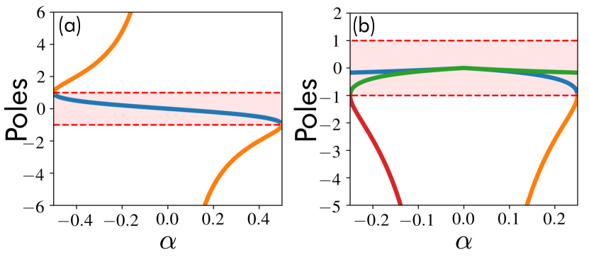
This expression can be computed with the help of the residue theorem by noting that, since , the integrand function always has a pole falling inside the unit circle at [see blue curve in 6(a)]. Calculating the corresponding residue we thus end up with
| (66) |
with the localization length given by Eq. (31).
C.2 2D case
In 2D and for a square geometry, (61) reduces to
| (67) |
with subject to the constraint (according to notation introduced in Eq. (60)) with . Plugging into Eq. (26) and taking the thermodynamic limit produces the double integral
| (68) |
where BZ stands for the region of integration specified by and . To evaluate the integral, we first take (i.e. we look at the behaviour of along the direction) which allows to write the integral as
| (69) |
which can be solved by applying the residue theorem twice, first to the integral over and then to that over . There occur four poles given by
| (70) |
with
| (71) |
We henceforth focus on the isotropic case with , which ensures that the localization length calculated along the -direction will be match the one along any other direction. In this isotropic case, the only two poles falling inside the unit circle are given by
| (72) |
Calculating the corresponding residues and summing up as prescribed by the residue theorem we thus end up with Eq. (33).
Appendix D BS localization length from
In this appendix, we show that the BS scales with distance BS in the same way as function defined in Eq. (26). For the sake of argument, we will focus on CLSs of class in 1D (the 2D case for is treated analogously on each of the two directions).
Let the state where a single photon lies on the th unit cell in the th sublattice. Since we assume , the CLS is localized only on two nearest-neighbour cells, say and , so that its wavefunction can be written as
| (73) |
where are the (in general complex) coefficients of the CLS in front of state . Replacing the above in the FB projector (25) this can be arranged as
| (74) |
If the atom is coupled to cavity , the BS wavefunction will be proportional to the following matrix element of [cf. Eq. (6)]
| (75) |
where and are constants.
Now, if (exponential shape), we get
| (76) |
This shows that in general this matrix element – hence the BS wavefunction – scales exponentially with the same localization length as function . An analogous result holds if is the sum of a finite number of exponentially localised terms.
The proof can be extended to CLSs of arbitrary class as long as the weight function scales as the sum of a finite number of exponentials.
References
- Roy et al. [2017] D. Roy, C. Wilson, and O. Firstenberg, Colloquium: Strongly interacting photons in one-dimensional continuum, Rev. Mod. Phys. 89, 021001 (2017).
- Chang et al. [2018] D. Chang, J. Douglas, A. González-Tudela, C.-L. Hung, and H. Kimble, Colloquium: Quantum matter built from nanoscopic lattices of atoms and photons, Rev. Mod. Phys. 90, 031002 (2018).
- Sheremet et al. [2023] A. S. Sheremet, M. I. Petrov, I. V. Iorsh, A. V. Poshakinskiy, and A. N. Poddubny, Waveguide quantum electrodynamics: Collective radiance and photon-photon correlations, Rev. Mod. Phys. 95, 015002 (2023).
- Ciccarello et al. [2024] F. Ciccarello, P. Lodahl, and D. Schneble, Waveguide Quantum Electrodynamics, Optics & Photonics News, OPN 35, 34 (2024).
- González-Tudela et al. [2024] A. González-Tudela, A. Reiserer, J. J. García-Ripoll, and F. J. García-Vidal, Light–matter interactions in quantum nanophotonic devices, Nat Rev Phys 6, 166 (2024).
- Bouscal et al. [2024] A. Bouscal, M. Kemiche, S. Mahapatra, N. Fayard, J. Berroir, T. Ray, J.-J. Greffet, F. Raineri, A. Levenson, K. Bencheikh, C. Sauvan, A. Urvoy, and J. Laurat, Systematic design of a robust half-W1 photonic crystal waveguide for interfacing slow light and trapped cold atoms, New J. Phys. 26, 023026 (2024).
- Goban et al. [2014] A. Goban, C.-L. Hung, S.-P. Yu, J. D. Hood, J. A. Muniz, J. H. Lee, M. J. Martin, A. C. McClung, K. S. Choi, D. E. Chang, O. Painter, and H. J. Kimble, Atom–light interactions in photonic crystals, Nat Commun 5, 3808 (2014).
- Zhou et al. [2023] X. Zhou, H. Tamura, T.-H. Chang, and C.-L. Hung, Coupling Single Atoms to a Nanophotonic Whispering-Gallery-Mode Resonator via Optical Guiding, Phys. Rev. Lett. 130, 103601 (2023).
- Menon et al. [2023] S. G. Menon, N. Glachman, M. Pompili, A. Dibos, and H. Bernien, An integrated atom array – nanophotonic chip platform with background-free imaging (2023).
- Jouanny et al. [2024] V. Jouanny, S. Frasca, V. J. Weibel, L. Peyruchat, M. Scigliuzzo, F. Oppliger, F. De Palma, D. Sbroggio, G. Beaulieu, O. Zilberberg, and P. Scarlino, Band engineering and study of disorder using topology in compact high kinetic inductance cavity arrays (2024).
- Liu and Houck [2017] Y. Liu and A. A. Houck, Quantum electrodynamics near a photonic bandgap, Nature Phys 13, 48 (2017).
- Mirhosseini et al. [2018] M. Mirhosseini, E. Kim, V. S. Ferreira, M. Kalaee, A. Sipahigil, A. J. Keller, and O. Painter, Superconducting metamaterials for waveguide quantum electrodynamics, Nat Commun 9, 3706 (2018).
- Scigliuzzo et al. [2022] M. Scigliuzzo, G. Calajò, F. Ciccarello, D. Perez Lozano, A. Bengtsson, P. Scarlino, A. Wallraff, D. Chang, P. Delsing, and S. Gasparinetti, Controlling Atom-Photon Bound States in an Array of Josephson-Junction Resonators, Phys. Rev. X 12, 031036 (2022).
- Lanuza et al. [2022] A. Lanuza, J. Kwon, Y. Kim, and D. Schneble, Multiband and array effects in matter-wave-based waveguide QED, Phys. Rev. A 105, 023703 (2022).
- Krinner et al. [2018] L. Krinner, M. Stewart, A. Pazmiño, J. Kwon, and D. Schneble, Spontaneous emission of matter waves from a tunable open quantum system, Nature 559, 589 (2018).
- Kim et al. [2021] E. Kim, X. Zhang, V. S. Ferreira, J. Banker, J. K. Iverson, A. Sipahigil, M. Bello, A. González-Tudela, M. Mirhosseini, and O. Painter, Quantum Electrodynamics in a Topological Waveguide, Phys. Rev. X 11, 011015 (2021).
- Owens et al. [2022] J. C. Owens, M. G. Panetta, B. Saxberg, G. Roberts, S. Chakram, R. Ma, A. Vrajitoarea, J. Simon, and D. I. Schuster, Chiral cavity quantum electrodynamics, Nat. Phys. 18, 1048 (2022).
- Kollár et al. [2019] A. J. Kollár, M. Fitzpatrick, and A. A. Houck, Hyperbolic lattices in circuit quantum electrodynamics, Nature 571, 45 (2019).
- Ritsch et al. [2013] H. Ritsch, P. Domokos, F. Brennecke, and T. Esslinger, Cold atoms in cavity-generated dynamical optical potentials, Rev. Mod. Phys. 85, 553 (2013).
- Zheng and Guo [2000] S.-B. Zheng and G.-C. Guo, Efficient Scheme for Two-Atom Entanglement and Quantum Information Processing in Cavity QED, Phys. Rev. Lett. 85, 2392 (2000).
- Douglas et al. [2015] J. S. Douglas, H. Habibian, C.-L. Hung, A. V. Gorshkov, H. J. Kimble, and D. E. Chang, Quantum many-body models with cold atoms coupled to photonic crystals, Nature Photon 9, 326 (2015).
- González-Tudela et al. [2015] A. González-Tudela, C.-L. Hung, D. E. Chang, J. I. Cirac, and H. J. Kimble, Subwavelength vacuum lattices and atom–atom interactions in two-dimensional photonic crystals, Nature Photon 9, 320 (2015).
- Sundaresan et al. [2019] N. M. Sundaresan, R. Lundgren, G. Zhu, A. V. Gorshkov, and A. A. Houck, Interacting Qubit-Photon Bound States with Superconducting Circuits, Phys. Rev. X 9, 011021 (2019).
- Zhang et al. [2023] X. Zhang, E. Kim, D. K. Mark, S. Choi, and O. Painter, A superconducting quantum simulator based on a photonic-bandgap metamaterial, Science 379, 278 (2023).
- Armon et al. [2021] T. Armon, S. Ashkenazi, G. García-Moreno, A. González-Tudela, and E. Zohar, Photon-mediated stroboscopic quantum simulation of a lattice gauge theory, Phys. Rev. Lett. 127, 250501 (2021).
- Bello et al. [2022] M. Bello, G. Platero, and A. González-Tudela, Spin many-body phases in standard- and topological-waveguide qed simulators, PRX Quantum 3, 010336 (2022).
- Tabares et al. [2022] C. Tabares, E. Zohar, and A. González-Tudela, Tunable photon-mediated interactions between spin-1 systems, Phys. Rev. A 106, 033705 (2022).
- Tabares et al. [2023] C. Tabares, A. Muñoz de las Heras, L. Tagliacozzo, D. Porras, and A. González-Tudela, Variational Quantum Simulators Based on Waveguide QED, Phys. Rev. Lett. 131, 073602 (2023).
- Lambropoulos et al. [2000] P. Lambropoulos, G. M. Nikolopoulos, T. R. Nielsen, and S. Bay, Fundamental quantum optics in structured reservoirs, Rep. Prog. Phys. 63, 455 (2000).
- Lombardo et al. [2014] F. Lombardo, F. Ciccarello, and G. M. Palma, Photon localization versus population trapping in a coupled-cavity array, Phys. Rev. A 89, 053826 (2014).
- Calajó et al. [2016] G. Calajó, F. Ciccarello, D. Chang, and P. Rabl, Atom-field dressed states in slow-light waveguide QED, Phys. Rev. A 93, 033833 (2016).
- Shi et al. [2016] T. Shi, Y.-H. Wu, A. González-Tudela, and J. Cirac, Bound States in Boson Impurity Models, Phys. Rev. X 6, 021027 (2016).
- González-Tudela and Cirac [2017] A. González-Tudela and J. I. Cirac, Markovian and non-Markovian dynamics of quantum emitters coupled to two-dimensional structured reservoirs, Phys. Rev. A 96, 043811 (2017).
- González-Tudela and Cirac [2018a] A. González-Tudela and J. I. Cirac, Exotic quantum dynamics and purely long-range coherent interactions in Dirac conelike baths, Phys. Rev. A 97, 043831 (2018a).
- González-Tudela and Cirac [2018b] A. González-Tudela and J. I. Cirac, Non-Markovian Quantum Optics with Three-Dimensional State-Dependent Optical Lattices, Quantum 2, 97 (2018b).
- González-Tudela and Galve [2019] A. González-Tudela and F. Galve, Anisotropic Quantum Emitter Interactions in Two-Dimensional Photonic-Crystal Baths, ACS Photonics 6, 221 (2019).
- Sánchez-Burillo et al. [2019] E. Sánchez-Burillo, L. Martín-Moreno, J. García-Ripoll, and D. Zueco, Single Photons by Quenching the Vacuum, Phys. Rev. Lett. 123, 013601 (2019).
- Román-Roche et al. [2020] J. Román-Roche, E. Sánchez-Burillo, and D. Zueco, Bound states in ultrastrong waveguide QED, Phys. Rev. A 102, 023702 (2020).
- Shi et al. [2018] T. Shi, Y.-H. Wu, A. González-Tudela, and J. I. Cirac, Effective many-body Hamiltonians of qubit-photon bound states, New J. Phys. 20, 105005 (2018).
- Leonforte et al. [2024] L. Leonforte, X. Sun, D. Valenti, B. Spagnolo, F. Illuminati, A. Carollo, and F. Ciccarello, Quantum optics with giant atoms in a structured photonic bath (2024).
- Vicencio Poblete [2021] R. A. Vicencio Poblete, Photonic flat band dynamics, Advances in Physics: X 6, 1878057 (2021).
- Leykam et al. [2018] D. Leykam, A. Andreanov, and S. Flach, Artificial flat band systems: from lattice models to experiments, Advances in Physics: X 3, 1473052 (2018).
- Klitzing et al. [1980] K. v. Klitzing, G. Dorda, and M. Pepper, New Method for High-Accuracy Determination of the Fine-Structure Constant Based on Quantized Hall Resistance, Phys. Rev. Lett. 45, 494 (1980).
- Danieli et al. [2024] C. Danieli, A. Andreanov, D. Leykam, and S. Flach, Flat band fine-tuning and its photonic applications (2024).
- Hu et al. [2023] J. Hu, X. Zhang, C. Hu, J. Sun, X. Wang, H.-Q. Lin, and G. Li, Correlated flat bands and quantum spin liquid state in a cluster Mott insulator, Commun Phys 6, 1 (2023).
- Rivas and Molina [2020] D. Rivas and M. I. Molina, Seltrapping in flat band lattices with nonlinear disorder, Sci Rep 10, 5229 (2020).
- Leykam et al. [2013] D. Leykam, S. Flach, O. Bahat-Treidel, and A. S. Desyatnikov, Flat band states: Disorder and nonlinearity, Phys. Rev. B 88, 224203 (2013).
- Rhim and Yang [2019] J.-W. Rhim and B.-J. Yang, Classification of flat bands according to the band-crossing singularity of Bloch wave functions, Phys. Rev. B 99, 045107 (2019).
- Chen et al. [2014] L. Chen, T. Mazaheri, A. Seidel, and X. Tang, The impossibility of exactly flat non-trivial Chern bands in strictly local periodic tight binding models, J. Phys. A: Math. Theor. 47, 152001 (2014).
- Read [2017] N. Read, Compactly supported Wannier functions and algebraic k-theory, Phys. Rev. B 95, 115309 (2017).
- Note [1] Atoms coupled to photonic FBs in specific models appeared in recent studies [70, 71, 72].
- Note [2] This is one of the two dressed states in the single-excitation sector, specifically the one with a dominant atomic component. The other state instead has energy and is mostly photonic.
- Economou [1979] E. N. Economou, Green’s Functions for Tight Binding Hamiltonians, in Green’s Functions in Quantum Physics, Springer Series in Solid-State Sciences, edited by E. N. Economou (Springer, Berlin, Heidelberg, 1979) pp. 71–91.
- Arfken et al. [2013] G. B. Arfken, H. J. Weber, and F. E. Harris, Chapter 10 - Green’s Functions, in Mathematical Methods for Physicists (Seventh Edition), edited by G. B. Arfken, H. J. Weber, and F. E. Harris (Academic Press, Boston, 2013) pp. 447–467.
- Note [3] If bath is not a lattice, a FB occurs when there exists a normal frequency with a thermodynamically large degeneracy. An instance of such a situation are certain kinds of hyperbolic systems, where there exists a FB gapped from the rest of the energy spectrum [18].
- Hyrkäs et al. [2013] M. Hyrkäs, V. Apaja, and M. Manninen, Many-particle dynamics of bosons and fermions in quasi-one-dimensional flat-band lattices, Phys. Rev. A 87, 023614 (2013).
- Sánchez-Burillo et al. [2020] E. Sánchez-Burillo, C. Wan, D. Zueco, and A. González-Tudela, Chiral quantum optics in photonic sawtooth lattices, Phys. Rev. Res. 2, 023003 (2020).
- Note [4] Strictly speaking, this is a special case of the sawtooth lattice in which the ratio of the two hopping rates is constrained so as to ensure the emergence of a FB.
- Bloch [1929] F. Bloch, Uber die Quantenmechanik der Elektronen in Kristallgittern, Z. Physik 52, 555 (1929).
- Wannier [1937] G. H. Wannier, The Structure of Electronic Excitation Levels in Insulating Crystals, Phys. Rev. 52, 191 (1937).
- Maimaiti et al. [2019] W. Maimaiti, S. Flach, and A. Andreanov, Universal d=1 flat band generator from compact localized states, Phys. Rev. B 99, 125129 (2019).
- Baboux et al. [2016] F. Baboux, L. Ge, T. Jacqmin, M. Biondi, E. Galopin, A. Lemaître, L. Le Gratiet, I. Sagnes, S. Schmidt, H. Türeci, A. Amo, and J. Bloch, Bosonic Condensation and Disorder-Induced Localization in a Flat Band, Phys. Rev. Lett. 116, 066402 (2016).
- Real et al. [2017] B. Real, C. Cantillano, D. López-González, A. Szameit, M. Aono, M. Naruse, S.-J. Kim, K. Wang, and R. A. Vicencio, Flat-band light dynamics in Stub photonic lattices, Sci Rep 7, 15085 (2017).
- Ramachandran et al. [2017] A. Ramachandran, A. Andreanov, and S. Flach, Chiral flat bands: Existence, engineering, and stability, Phys. Rev. B 96, 161104 (2017).
- Lieb [1989] E. H. Lieb, Two theorems on the Hubbard model, Phys. Rev. Lett. 62, 1201 (1989).
- Note [5] This zero-energy FB always exists in lattices with chiral symmetry and an odd number of sublattices (Lieb’s Theorem [65]). This is because chiral energy imposes the energy spectrum to be symmetric around for any . As the total number of energy bands is odd, one of the bands must necessarily be a zero-energy FB.
- Mekata [2003] M. Mekata, Kagome: The Story of the Basketweave Lattice, Physics Today 56, 12 (2003).
- Note [6] Unlike previous examples of overlapping CLSs, the set (36) is not a complete basis of the FB eigenspace, which can be shown to be due to the singular behaviour of the present FB [48]. To get a complete basis, the set (36) must be complemented with a pair of so called non-contractible loop states [see 5(b)]. These two states are yet unbound, hence in the thermodynamic limit we can neglect their contribution to the BS (this arising from the local atom-field interaction).
- Frisk Kockum [2021] A. Frisk Kockum, Quantum Optics with Giant Atoms—the First Five Years, in International Symposium on Mathematics, Quantum Theory, and Cryptography, Mathematics for Industry, edited by T. Takagi, M. Wakayama, K. Tanaka, N. Kunihiro, K. Kimoto, and Y. Ikematsu (Springer, Singapore, 2021) pp. 125–146.
- De Bernardis et al. [2021] D. De Bernardis, Z.-P. Cian, I. Carusotto, M. Hafezi, and P. Rabl, Light-Matter Interactions in Synthetic Magnetic Fields: Landau-Photon Polaritons, Phys. Rev. Lett. 126, 103603 (2021).
- Bienias et al. [2022] P. Bienias, I. Boettcher, R. Belyansky, A. J. Kollár, and A. V. Gorshkov, Circuit Quantum Electrodynamics in Hyperbolic Space: From Photon Bound States to Frustrated Spin Models, Phys. Rev. Lett. 128, 013601 (2022).
- De Bernardis et al. [2023] D. De Bernardis, F. S. Piccioli, P. Rabl, and I. Carusotto, Chiral Quantum Optics in the Bulk of Photonic Quantum Hall Systems, PRX Quantum 4, 030306 (2023).