Recurrent neural network wave functions for Rydberg atom arrays on kagome lattice
Abstract
Rydberg atom array experiments have demonstrated the ability to act as powerful quantum simulators, preparing strongly-correlated phases of matter which are challenging to study for conventional computer simulations. A key direction has been the implementation of interactions on frustrated geometries, in an effort to prepare exotic many-body states such as spin liquids and glasses. In this paper, we apply two-dimensional recurrent neural network (RNN) wave functions to study the ground states of Rydberg atom arrays on the kagome lattice. We implement an annealing scheme to find the RNN variational parameters in regions of the phase diagram where exotic phases may occur, corresponding to rough optimization landscapes. For Rydberg atom array Hamiltonians studied previously on the kagome lattice, our RNN ground states show no evidence of exotic spin liquid or emergent glassy behavior. In the latter case, we argue that the presence of a non-zero Edwards-Anderson order parameter is an artifact of the long autocorrelations times experienced with quantum Monte Carlo simulations. This result emphasizes the utility of autoregressive models, such as RNNs, to explore Rydberg atom array physics on frustrated lattices and beyond.
I Introduction
Rydberg atom arrays have emerged as a rich playground for quantum simulation of many-body problems Browaeys and Lahaye (2020). A key property of these arrays is their high degree of programmability, which enables the realization of multiple Hamiltonians on different lattice geometries and parameter ranges. This programmability facilitates the simulation of a wide array of phases of matter Ebadi et al. (2021); Wurtz et al. (2023) and enables the solution to challenging combinatorial optimization problems Wurtz et al. (2023); Ebadi et al. (2022); Nguyen et al. (2023). Remarkably, the preparation of spin liquid phases—disordered phases of matter characterized by the presence of anyonic excitations, topological invariants, and long-range entanglement—has been demonstrated in programmable Rydberg arrays, potentially serving as building blocks of future generation of fault-tolerant qubits Dennis et al. (2002); Kitaev (2006); Kitaev and Laumann (2009).
Recent numerical studies have investigated the physics of the ground state of Rydberg atom arrays in different lattice geometries, in particular in one Samajdar et al. (2018) and two spatial dimensions in various geometries Samajdar et al. (2020); Kalinowski et al. (2022); Li et al. (2022); Samajdar et al. (2021); Verresen et al. (2021); Yang and Xu (2022); Kornjača et al. (2023). In lattices such as ruby and honeycomb lattices, strong numerical evidence favours the existence of a spin liquid phase in agreement with experiments Verresen et al. (2021); Kornjača et al. (2023). Another recent example is the kagome lattice, where Density Matrix Renormalization Group (DMRG) White (1992); Schollwöck (2011) studies provided evidence that Rydberg atom arrays host a liquid-like regime Samajdar et al. (2021), while Quantum Monte Carlo (QMC) simulations predicted the existence of a spin glass phase Yan et al. (2023). These systems display frustration arising from lattice geometry and Hamiltonian interactions, leading to the existence of a large number of quantum states with nearly degenerate energies but markedly different properties. This makes it computationally difficult to accurately approximate the ground state of these systems.
Here we focus on applying recurrent neural network (RNNs) wave functions Hibat-Allah et al. (2020); Roth (2020) to a Rydberg array of atoms on the kagome lattice. The effectiveness of RNNs and Transformer language models has already been demonstrated in Rydberg atom arrays on the square lattice Moss et al. (2023); Sprague and Czischek (2023); Czischek et al. (2022). RNNs possess two key properties that make them particularly well-suited for studying frustrated systems. Firstly, their ability to perform exact sampling helps mitigate frustration-induced ergodicity issues in quantum Monte Carlo. Secondly, the ability to define them in any spatial dimension without incurring additional computational intractability helps address challenges faced by techniques like DMRG, such as the increased computational cost stemming from increased entanglement in higher dimensions Hibat-Allah et al. (2020, 2022).
Our findings reveal that in the highly frustrated and highly entangled regimes of the system, the RNN predicts a paramagnetic phase without topological order, consistent with earlier QMC simulations Yan et al. (2023). However, in contrast to the QMC results in Ref. Yan et al., 2023, the RNN suggests the absence of a spin-glass phase. Nevertheless, in agreement with QMC, our numerical simulations indicate the emergence of a rugged optimization landscape, necessitating more optimization steps and thermal-like fluctuations to mitigate local minima in the RNN’s parameter landscape.
Overall, our results showcase the remarkable applicability and advantages of machine learning-based wave functions, particularly RNNs, in tackling challenging problems at the forefront of Rydberg atom array physics. These findings pave the way for further exploration of exotic phases and phenomena in highly frustrated quantum systems, harnessing the power of modern machine learning techniques to advance our understanding in this field.
II Methods
We focus our attention on an array of neutral atoms on the kagome lattice, interacting via laser excitation to atomic Rydberg states. We consider a lattice with periodic boundary conditions (PBC). The Hamiltonian of this system is given by Browaeys and Lahaye (2020); Samajdar et al. (2021):
Here are respectively the ground and excited states of the Rydberg atom . is the Rabi frequency and is the laser detuning. is the repulsive potential due to the dipole-dipole interaction between Rydberg atoms, which is responsible for the blockade mechanism Browaeys and Lahaye (2020). In practice, we define a blockade radius such that , where is the distance between two neighbouring Rydberg atoms. Finally, we note that the sum over all possible pairs is truncated to a sum over neighbors separated by a distance cutoff or . The choice is taken to compare with the DMRG results reported in Ref. Samajdar et al. (2021) as well as with the QMC findings in Ref. Yan et al. (2023).
II.1 Two dimensional RNNs
The Rydberg Hamiltonian is stoquastic in nature Bravyi (2015), which implies that the ground-state wave function contains only positive amplitudes. This offers the opportunity to model the ground state with an RNN wave function with only positive amplitudes Hibat-Allah et al. (2020) which we adopt below. Complex extensions of RNN wave functions for non-stoquastic Hamiltonians have been explored in Refs. Hibat-Allah et al. (2020); Roth (2020); Hibat-Allah et al. (2022). To model a positive RNN wave function, we can express our ansatz in the computational basis as:
such that corresponds to the variational parameters of the ansatz , and is a configuration of the Rydberg atoms. The main advantage of using RNN wave functions is the possibility of estimating observables through autoregressive sampling, which allows obtaining uncorrelated samples by construction Hibat-Allah et al. (2020). To do so, we model the joint probability by constructing the conditionals by taking advantage of the probability chain rule
These conditional probabilities are obtained through a Softmax layer as follows:
Here where and are, respectively, trainable weights and biases, and ‘Softmax’ corresponds to the normalizing Softmax activation function. Additionally, the memory (hidden) state is obtained recursively as Lipton et al. (2015):
| (1) |
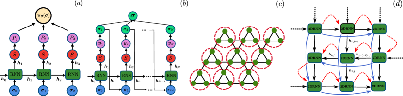
such that is a concatenation of two vectors, while is a one-hot encoding of . These computations are illustrated in Fig. 1(a). and are also trainable weights and biases, and is a user-defined activation function.
By virtue of the ‘Softmax’ activation function, the conditionals are normalized to one. This property implies that the RNN joint probability is also normalized Hibat-Allah et al. (2020). Furthermore, by sampling the conditionals sequentially, as illustrated in Fig. 1(b), we can extract exact samples from the joint RNN probability . An attractive property of this scheme is the possibility to efficiently generate uncorrelated samples from different modes present in , whereas traditional Metropolis sampling scheme may get stuck in only one mode.
The atom configurations of a Rydberg atom array on a kagome lattice can be seen as an array of binary degrees of freedom where is the size of each side of the lattice. As illustrated in Fig. 1(c), we can map our kagome lattice with a local Hilbert space of to a square lattice with an enlarged Hilbert space of size which we can study using our two-dimensional (2D) RNN wave function Hibat-Allah et al. (2023); Sprague and Czischek (2023).
To construct a 2D RNN ansatz that can handle PBC, we modify our RNN recursion in Eq. (1) to a two-dimensional recursion relation as:
| (2) |
is a memory state with two indices for each atom in the two-dimensional lattice. Here ‘Neighbours()’ returns a concatenation of the neighbours of . The same observation goes for ‘Neighbours()’. These neighbours correspond to incoming vectors indicated by the black and blue arrows as illustrated in Fig. 1(d). More specifically, we define
on the bulk. On the boundaries, we take
Note that PBC on the indices is assumed. The additional inputs , and hidden states , allow to take PBC into account and to introduce correlations between degrees of freedom at the boundaries. During the autoregressive sampling procedure, the input and hidden vectors are initialized to a null vector if not previously defined to preserve the autoregressive nature of our scheme, as illustrated in Fig. 1(b). Also, note that the particular choice of the indices is motivated by the zigzag sampling path. In this study, we use an advanced version of 2D RNNs incorporating the gating mechanism as previously done in Refs. Hibat-Allah et al. (2022); Casert et al. (2021); Luo et al. (2023). More details can be found in Appendix. A. Finally, since is a summary of the history of the generated , it is used to compute the conditional probabilities as follows:
| (3) |
II.2 Supplementing RNN optimization with annealing
To reach the ground state of the Rydberg atoms array Hamiltonian on the kagome lattice, we minimize the energy expectation value using the Variational Monte Carlo (VMC) scheme Becca and Sorella (2017) (see Appendix B). Due to the frustrated nature of the kagome lattice which can induce local minima in the VMC scheme, we leverage annealing with thermal-like fluctuations to mitigate local minima. This technique has been suggested and implemented in Refs. Roth (2020); Hibat-Allah et al. (2021, 2022); Roth et al. (2022); Khandoker et al. (2023); Hibat-Allah et al. (2023). In this case, we obtain a free-energy like cost function, defined as
| (4) |
where is a variational pseudo Free energy and is the classical Shannon entropy:
| (5) |
The previous sum goes over all classical Rydberg configurations in the computational -basis. Note that is a pseudo-entropy that can be efficiently estimated using our RNN wave function as opposed to the quantum von Neumann entropy. Additionally, is a pseudo-temperature that is annealed from some initial value to zero as follows: where and is the total number of annealing steps. We present more details about the hyperparameters of our training scheme in Appendix. C.
II.3 Topological entanglement entropy
To investigate the existence of a topological property in the Rydberg atom arrays on the kagome lattice, we compute the topological entanglement entropy (TEE) Hamma et al. (2005a, b); Levin and Wen (2006); Kitaev and Preskill (2006); Flammia et al. (2009); Isakov et al. (2011); Wildeboer et al. (2017). For a gapped phase of matter, where the area law is satisfied, the Renyi- entanglement entropy follows the scaling law , assuming and is partition of the system, is the size of the boundary between and and . In this case, is the so-called TEE. In this paper, we use the swap trick with our RNN wave function ansatz Hastings et al. (2010); Hibat-Allah et al. (2020); Wang and Davis (2020) to calculate the second Renyi entropy to extract the TEE .
We extract using two different strategies, namely the Kitaev-Preskill construction Kitaev and Preskill (2006) and the Levin-Wen construction Levin and Wen (2006), illustrated in Fig. 2.
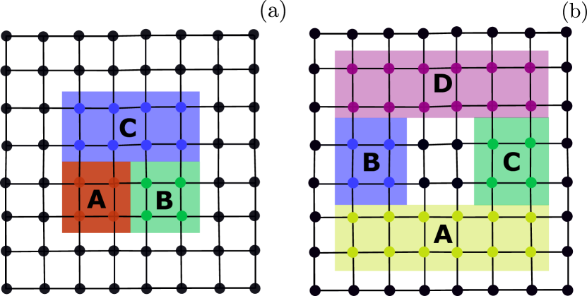
The Kitaev-Preskill construction consists of choosing three subregions , , with geometries as shown in Fig. 2(a). The TEE can be then obtained by computing
where is the second Renyi entropy of the subsystem , and is the union of and and similarly for the other terms. It is worth mentioning that finite size effects on can be reduced by extrapolating the size of the subregions Kitaev and Preskill (2006); Furukawa and Misguich (2007). Finally, note that this approach combined with RNN wave functions was successful in extracting a non-zero TEE on the toric code and the hard-core Bose-Hubbard model on the kagome lattice Hibat-Allah et al. (2023).
The Levin-Wen construction allows to extract the TEE by constructing four different subsystems and as illustrated in Fig. 2(b) such that Isakov et al. (2011):
Note that finite size effects on can be reduced by extrapolating the width and thickness of and Isakov et al. (2011); Furukawa and Misguich (2007).
Finally, we would like to highlight that our ability to study quantum systems with fully periodic boundary conditions is key to mitigating boundary effects, as opposed to cylinders used in DMRG Stoudenmire and White (2012); Gong et al. (2014), which can introduce boundary effects in the TEE value Samajdar et al. (2021).
III Results
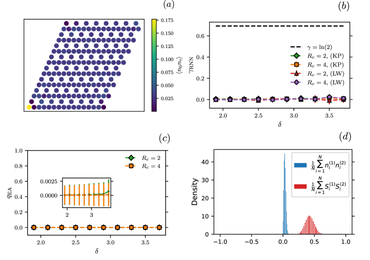
According to the RNN numerics, our results show that the ground state at and , which is suggested to be in the spin-liquid phase according to Ref. Samajdar et al. (2021), is rather a disordered state with no topological order. We first plot the correlations in Fig. 3(a). The results indicate that the extracted state has short-range correlations. To confirm the correctness of our variational implementation, we perform a sanity check and compare our ground state energies with QMC and DMRG as shown in Appendix D. We found a good agreement between our RNN energies and QMC as well as DMRG energies. Most importantly, we observe that our RNN results using only are more accurate compared to DMRG with a bond dimension in the highly entangled regime at and .
To investigate the existence of a spin liquid in this regime, we calculate the TEE using the Kitaev-Preskill construction Kitaev and Preskill (2006) for a system size (see Fig. 2(a)), and for different values of and at . We also do the same using the Levin-Wen construction Isakov et al. (2011) in Fig. 2(b). Our results, illustrated in Fig. 3(b) suggest that the TEE extracted by the RNN is consistent with zero and different from within error bars. These results suggest the non-existence of a spin liquid within our settings and also suggest that the state we find in this regime is a disordered state. Our findings are further corroborated by a recent QMC study Yan et al. (2023) and also by previous results in the literature suggesting that the paramagnetic ‘liquid’ phase in Ising systems on the kagome lattice is not exotic Nikolić and Senthil (2005); Moessner and Sondhi (2001); Moessner et al. (2000).
In this QMC study Yan et al. (2023), it was suggested that the region, around and the values of used in our study, contains an emergent spin-glass phase instead of a paramagnetic state. To verify this claim, we compute the Edwards-Anderson (EA) order parameters Edwards and Anderson (1975); Richards (1984), defined as:
| (6) |
where is the system size, is the occupation number of site and . Deviations of this order parameter from zero values are signals of the existence of a spin-glass phase. In Fig. 3(c), we plot this order parameter as a function of with and . We find that the values of the order parameter are consistent with zero, as opposed to the results of QMC in Ref. Yan et al. (2023). Furthermore, we report in Fig. 3(d) the density-density overlap and the spin-spin overlap between different RNN samples at , and . Here labels (1) and (2) correspond to two independent sets of samples, which are obtained from optimized RNNs with different training seeds. The Gaussian nature of the overlap distribution in both representations is another indicator that there is no static signature of a spin-glass order Castellani and Cavagna (2005).
The discrepancy in our results and previous QMC findings Yan et al. (2023) could be related to emergent glassy dynamics in the QMC simulations, which results in very long auto-correlations times and thus in a non-ergodic behavior. To corroborate our findings, we run QMC simulations Merali et al. (2023) for larger inverse temperatures compared to Ref. Yan et al. (2023), namely for and using Monte Carlo samples. We find that the QMC prediction for the EA order parameter is given as for , a system size , and for a radius cutoff . The previous result agrees very well with our RNN findings in Fig. 3(c). This result is also confirmed by the good agreement between the RNN energies and the QMC energies as shown in Appendix. D. Our findings are further supported by the results of Ref. Yan et al. (2022), which suggests the possibility of transition in a quantum dimer model between nematic to paramagnetic to staggered states. In conclusion, our numerical investigation suggests that the long auto-correlation time could be a limiting factor in the QMC results reported in Ref. Yan et al. (2023).
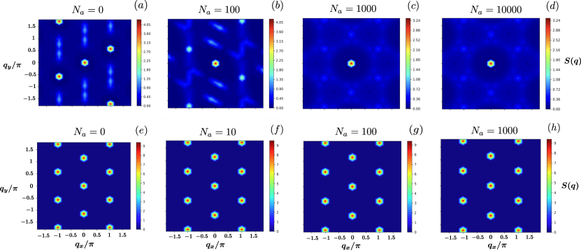
We note that the emergence of a long autocorrelation time in QMC coincides with the emergence of a rugged optimization landscape, which in our simulations implies a longer number of annealing steps in our RNN simulations to achieve convergence. To demonstrate this point, we compute the structure factor
| (7) |
to extract the nature of the states obtained by our RNN ansatz and investigate their dependence on the number of annealing steps . We expect the optimization landscape to be rougher as required to converge increases. Figs. 4(a-d) at and show that the RNN finds different states for different numbers of annealing steps , until it converges to a state without ordering peaks, i.e., the paramagnetic state. In contrast, the nematic state at can be reached without the need for annealing, as illustrated by the structure factors at different in Fig. 4(e-h). These observations suggest an emergent rugged optimization landscape when optimizing our ansatz in the highly entangled regime. Finally, to find the optimal number of annealing steps in the highly entangled regime, we note that we conduct a scaling study as shown in Appendix E.
IV Conclusions and Outlooks
In this paper, we demonstrate a successful application of recurrent neural network (RNN) wave functions to the task of investigating topological order on Rydberg atom arrays on kagome lattice. We use these architectures to estimate the second Renyi entropies using the swap trick Hibat-Allah et al. (2020). The latter allows us to compute the TEEs using the Kitaev-Preskill Kitaev and Preskill (2006) and the Levin-Wen Levin and Wen (2006) constructions. Furthermore, with the possibility of handling periodic boundary conditions in RNNs, the boundary effects on the TEE are reduced compared to DMRG, which has challenges with boundary effects on cylinders Gong et al. (2014).
Our main finding, suggested by the two-dimensional RNN wave functions results, points out that Rydberg atom arrays on the kagome lattice do not establish a spin liquid in the highly entangled regime. This observation is also consistent with previous QMC studies Yan et al. (2023). Our RNN numerics also suggest that the highly entangled region corresponds to a trivial paramagnetic state and that there is no signature for spin glass order as opposed to the observations outlined in Ref. Yan et al. (2023). We believe that the ability of RNNs to generate uncorrelated samples from a multimodal distribution is a crucial factor in ruling out the spin-glass phase. Furthermore, supplementing RNNs with annealing turns out to be a valuable tool for mitigating local minima induced by the frustrated nature of the kagome lattice in the highly entangled regime. Additionally, we conclude that autocorrelation could be the main factor behind the observed spin glass phase observed in previous QMC simulations Yan et al. (2023).
Finally, we note that our method can be generalized to study other systems with potential topological order, such as the Rydberg atom arrays on the Ruby lattice Verresen et al. (2021); Semeghini et al. (2021); Giudici et al. (2022). One could also use quantum state tomography with RNNs Carrasquilla et al. (2019) in a wide variety of quantum simulators and also combine data with VMC to improve the variational results Bennewitz et al. (2021); Czischek et al. (2022); Moss et al. (2023). We also believe in the potential of RNN wave functions ansätzes in the discovery of new phases of matter with topological order. Overall, these results highlight the promising future of RNN wave functions Hibat-Allah et al. (2020); Roth (2020), language-model based wave functions, and neural quantum states Carleo and Troyer (2017) for investigating open questions and discovering new physics within the condensed matter community and beyond.
Code Availability
Our code is made publicly available at “http://github.com/mhibatallah/RNNWavefunctions”. The hyperparameters we use are given in Appendix. C.
Acknowledgments
We would like to thank Subir Sachdev, Anders Sandvik, and Arun Paramekanti for their helpful and inspiring discussions. Our RNN implementation is based on Tensorflow Abadi et al. (2015) and NumPy Harris et al. (2020). Computer simulations were made possible thanks to the Vector Institute computing cluster and the Digital Research Alliance of Canada cluster. We acknowledge support from Natural Sciences and Engineering Research Council of Canada (NSERC), the Shared Hierarchical Academic Research Computing Network (SHARCNET), Compute Canada, and the Canadian Institute for Advanced Research (CIFAR) AI chair program. This work is not related to the research being performed at AWS. Research at Perimeter Institute is supported in part by the Government of Canada through the Department of Innovation, Science and Economic Development and by the Province of Ontario through the Ministry of Colleges and Universities. This research was supported in part by grant NSF PHY-2309135 to the Kavli Institute for Theoretical Physics (KITP).
Appendix A Two dimensional periodic gated RNNs
In this Appendix, we share more details about our 2D gated RNN wave function implementation for periodic systems, which is used in this study to target the ground states of the Rydberg atom arrays on the kagome lattice. If we define
then our gated 2D RNN wave function ansatz is based on the following recursion relations:
A hidden state can be obtained by combining a candidate state and the neighbouring hidden states . The update gate determines how much of the candidate hidden state will be taken into account and how much of the neighboring states will be considered. With this combination, it is possible to mitigate some limitations of the vanishing gradient problems Zhou et al. (2016); Shen (2019). The weight matrices and the biases are variational parameters of our RNN ansatz in addition to the Softmax layer parameters in Eq. (3). Note that we choose the size of the hidden state , which we denote as , before optimizing our ansatz parameters. We note that the choice of the gated 2DRNN is motivated by its superiority compared to the non-gated 2DRNN on the task of finding the ground state of the 2D Heisenberg model Hibat-Allah et al. (2022).
Since we use an enlarged local Hilbert space with three atoms at each recursion step, the size of the Softmax layer output is defined as . Additionally, each input is defined as a concatenation of the one-hot encoding of each of the three atoms. This means that is a six-dimensional vector.
Appendix B Variational monte carlo (VMC)
To optimize the energy expectation value of our RNN wave function , we use the Variational Monte Carlo (VMC) scheme, which consists of using importance sampling to estimate the energy expectation value as follows Becca and Sorella (2017); Hibat-Allah et al. (2020):
where the local energies are defined as
Here the configurations are sampled from our ansatz using autoregressive sampling. The choice of is a hyperparameter that can be tuned. Similarly, the gradients can be estimated as
Subtracting the mean energy is helpful to achieve convergence as it reduces the variance of the gradients without biasing its expectation value Hibat-Allah et al. (2020, 2023). The gradient descent steps are performed using the Adam optimizer Kingma and Ba (2015). Similarly to the stochastic energy estimation, we can implement a similar procedure for the estimation of the variational pseudo-free energy in Eq. (4). Ref. Hibat-Allah et al. (2021) provides more details in the supplementary information.
Appendix C Hyperparameters
For all models studied in this paper, we note that for each annealing step, we perform gradient steps. Concerning the learning rate , we choose during the warm-up phase and the annealing phase and switch to a learning rate in the convergence phase. To train RNN on the lattices, we pre-train using the optimized RNN on the lattice without using annealing, since the RNN is expected to start from a variational energy that is close to the ground state energy in the new system size.
In Tab. 1, we provide further details about the hyperparameters we choose in our study for the different models. For the estimation of the RNN energy, we use independent configurations. We also use independent samples for the estimation of the entanglement entropy along with their error bars. For the estimation of the TEE using Kitaev-Preskill or Levin-Wen constructions, we use the expression of the standard deviation of the sum of independent random variables to estimate the one standard deviation on .
| Figures | Parameter | Value |
| Fig. 3 () | Number of memory units | |
| Number of training samples | ||
| Initial pseudo-temperature | ||
| Number of warm-up steps | ||
| Number of annealing steps | ||
| Number of convergence steps | ||
| Number of samples for TEE estimation | ||
| Number of samples for estimation | ||
| Fig. 3 () | Number of memory units | |
| Number of training samples | ||
| Initial pseudo-temperature | ||
| Number of warm-up steps | ||
| Number of annealing steps | (pre-trained from ) | |
| Number of training steps | ||
| Fig. 4 () | Number of memory units | |
| Number of training samples | ||
| Initial pseudo-temperature | ||
| Number of warm-up steps | ||
| Number of convergence steps | ||
| Number of sample for two-point correlations estimation | ||
| Fig. 5 () | Number of memory units | |
| Number of training samples | ||
| Initial pseudo-temperature | ||
| Number of warm-up steps | ||
| Number of convergence steps | ||
| Number of samples for energy and density estimation | ||
| Number of samples for estimation |
Appendix D Numerical comparisons
In Tab. 2, we show a comparison between QMC’s and RNN’s energies per site for a system size and for a detuning and at the blockade radiuses . These points correspond to the nematic and disordered phases, respectively. We note that our RNN-based ansatz provides energies with a relative error of less than compared to the QMC energies. The QMC simulations we run for Rydberg atom arrays are introduced in Ref. Merali et al. (2023). We use a finite-temperature QMC scheme run at several different values of until we observe convergence to the ground state. For each , five independent simulations are taken and the convergence of observables is observed at . Thus, to compute observables, we treat simulations with as additional independent chains, giving us a total of 25 independent Markov chains at each parameter point. Each chain is allowed to warm-up for steps, after which sequential measurements were taken. With respect to the computation of the Edwards-Anderson order parameter, , we note that the analysis given in Ref. Yan et al. (2023) can give different results in the case of imperfect sampling. Ref. Yan et al. (2023) computes the order parameter independently for each Markov chain and then averages the results. This procedure can produce different results as each chain will only explore a subset of the QMC configuration space due to the presence of frustrated interactions. As a result, each chain’s estimate of the one-point function can be biased. Since is a non-linear function of the one-point function, we must first aggregate the one-point functions generated by each Markov chain, and then compute . Lastly, to compute an estimate of the error in , we must account for auto-correlations and non-linearity simultaneously. This step is done by combining jackknife resampling with a binning procedure. To deal with auto-correlations, we first compute the one-point function on sequential “bins” of data; we found a bin size of to be sufficient, giving bins for each chain. Thus, we can consider each bin’s one-point function to be nearly uncorrelated, allowing us to directly apply the jackknife resampling procedure to these approximately independent bins.
To compare our RNN wave function () results with DMRG, we perform DMRG simulations using PastaQ Torlai and Fishman (2020) and ITensor Fishman et al. (2022) to further check the consistency of our RNN energies. In Tab. 3, we compare with DMRG using periodic boundary conditions. In the nematic phase , we find an excellent match of the energies. For the disordered phase at , our RNN energies are lower within an error of about and with orders of magnitude fewer parameters compared to DMRG. Furthermore, we choose the YC12 geometry used in Ref. Samajdar et al. (2021). We optimize our 2DRNN wave function () at and . Our estimated energy is which is within 0.3% error compared to the DMRG energy provided in Ref. Samajdar et al. (2021).
| QMC () | 2DRNN () | QMC () | 2DRNN () | |
| -0.79056(1) | -0.790964(5) | -0.77546(1) | -0.775412(4) | |
| -0.59785(1) | -0.59657(1) | -0.56445(1) | -0.56401(3) |
| Rydberg parameters | DMRG () | 2DRNN () |
| -0.790957 | -0.790934(7) | |
| -0.593828 | -0.59700(4) |
Appendix E Annealing and local minima
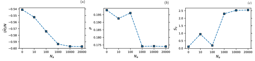
In Fig. 5, we demonstrate the importance of incorporating annealing in the training of RNNs applied to Rydberg atom arrays on the kagome lattice. These experiments are carried out in the highly entangled regime at and . In panel (a), we observe that the ground state energy improves with more annealing steps . We also highlight that the density saturates close to , which raises the possibility of an odd quantum spin liquid Yan et al. (2023); Samajdar et al. (2021). However, it is not a sufficient condition as this phase is found to be the paramagnetic state according to our RNN numerics. We also outline a saturation of the second Renyi entropy to a large value in the asymptotic limit of . All these numerics suggest that is a good choice to converge our RNN training.
References
- Browaeys and Lahaye (2020) Antoine Browaeys and Thierry Lahaye, “Many-body physics with individually controlled Rydberg atoms,” Nature Physics 16, 132–142 (2020).
- Ebadi et al. (2021) Sepehr Ebadi, Tout T. Wang, Harry Levine, Alexander Keesling, Giulia Semeghini, Ahmed Omran, Dolev Bluvstein, Rhine Samajdar, Hannes Pichler, Wen Wei Ho, Soonwon Choi, Subir Sachdev, Markus Greiner, Vladan Vuletić, and Mikhail D. Lukin, “Quantum phases of matter on a 256-atom programmable quantum simulator,” Nature 595, 227–232 (2021).
- Wurtz et al. (2023) Jonathan Wurtz, Alexei Bylinskii, Boris Braverman, Jesse Amato-Grill, Sergio H. Cantu, Florian Huber, Alexander Lukin, Fangli Liu, Phillip Weinberg, John Long, Sheng-Tao Wang, Nathan Gemelke, and Alexander Keesling, “Aquila: Quera’s 256-qubit neutral-atom quantum computer,” (2023), arXiv:2306.11727 [quant-ph] .
- Ebadi et al. (2022) S. Ebadi, A. Keesling, M. Cain, T. T. Wang, H. Levine, D. Bluvstein, G. Semeghini, A. Omran, J.-G. Liu, R. Samajdar, X.-Z. Luo, B. Nash, X. Gao, B. Barak, E. Farhi, S. Sachdev, N. Gemelke, L. Zhou, S. Choi, H. Pichler, S.-T. Wang, M. Greiner, V. Vuletić, and M. D. Lukin, “Quantum optimization of maximum independent set using rydberg atom arrays,” Science 376, 1209–1215 (2022), https://www.science.org/doi/pdf/10.1126/science.abo6587 .
- Nguyen et al. (2023) Minh-Thi Nguyen, Jin-Guo Liu, Jonathan Wurtz, Mikhail D. Lukin, Sheng-Tao Wang, and Hannes Pichler, “Quantum optimization with arbitrary connectivity using rydberg atom arrays,” PRX Quantum 4 (2023), 10.1103/prxquantum.4.010316.
- Dennis et al. (2002) Eric Dennis, Alexei Kitaev, Andrew Landahl, and John Preskill, “Topological quantum memory,” Journal of Mathematical Physics 43, 4452–4505 (2002).
- Kitaev (2006) Alexei Kitaev, “Anyons in an exactly solved model and beyond,” Annals of Physics January Special Issue, 321, 2–111 (2006).
- Kitaev and Laumann (2009) Alexei Kitaev and Chris Laumann, “Topological phases and quantum computation,” (2009), arXiv:0904.2771 [cond-mat.mes-hall] .
- Samajdar et al. (2018) Rhine Samajdar, Soonwon Choi, Hannes Pichler, Mikhail D. Lukin, and Subir Sachdev, “Numerical study of the chiral quantum phase transition in one spatial dimension,” Phys. Rev. A 98, 023614 (2018).
- Samajdar et al. (2020) Rhine Samajdar, Wen Wei Ho, Hannes Pichler, Mikhail D. Lukin, and Subir Sachdev, “Complex density wave orders and quantum phase transitions in a model of square-lattice rydberg atom arrays,” Physical Review Letters 124 (2020), 10.1103/physrevlett.124.103601.
- Kalinowski et al. (2022) Marcin Kalinowski, Rhine Samajdar, Roger G. Melko, Mikhail D. Lukin, Subir Sachdev, and Soonwon Choi, “Bulk and boundary quantum phase transitions in a square rydberg atom array,” Phys. Rev. B 105, 174417 (2022).
- Li et al. (2022) Chang-Xiao Li, Sheng Yang, and Jing-Bo Xu, “Quantum phases of rydberg atoms on a frustrated triangular-lattice array,” Opt. Lett. 47, 1093–1096 (2022).
- Samajdar et al. (2021) Rhine Samajdar, Wen Wei Ho, Hannes Pichler, Mikhail D. Lukin, and Subir Sachdev, “Quantum phases of rydberg atoms on a kagome lattice,” Proceedings of the National Academy of Sciences 118, e2015785118 (2021).
- Verresen et al. (2021) Ruben Verresen, Mikhail D. Lukin, and Ashvin Vishwanath, “Prediction of toric code topological order from rydberg blockade,” Physical Review X 11 (2021), 10.1103/physrevx.11.031005.
- Yang and Xu (2022) Sheng Yang and Jing-Bo Xu, “Density-wave-ordered phases of rydberg atoms on a honeycomb lattice,” Phys. Rev. E 106, 034121 (2022).
- Kornjača et al. (2023) Milan Kornjača, Rhine Samajdar, Tommaso Macrì, Nathan Gemelke, Sheng-Tao Wang, and Fangli Liu, “Trimer quantum spin liquid in a honeycomb array of rydberg atoms,” Communications Physics 6, 358 (2023).
- White (1992) Steven R. White, “Density matrix formulation for quantum renormalization groups,” Phys. Rev. Lett. 69, 2863–2866 (1992).
- Schollwöck (2011) Ulrich Schollwöck, “The density-matrix renormalization group in the age of matrix product states,” Annals of Physics 326, 96–192 (2011).
- Yan et al. (2023) Zheng Yan, Yan-Cheng Wang, Rhine Samajdar, Subir Sachdev, and Zi Yang Meng, “Emergent glassy behavior in a kagome rydberg atom array,” Phys. Rev. Lett. 130, 206501 (2023).
- Hibat-Allah et al. (2020) Mohamed Hibat-Allah, Martin Ganahl, Lauren E. Hayward, Roger G. Melko, and Juan Carrasquilla, “Recurrent neural network wave functions,” Physical Review Research 2 (2020), 10.1103/physrevresearch.2.023358.
- Roth (2020) Christopher Roth, “Iterative retraining of quantum spin models using recurrent neural networks,” (2020), arXiv:2003.06228 [physics.comp-ph] .
- Moss et al. (2023) M. Schuyler Moss, Sepehr Ebadi, Tout T. Wang, Giulia Semeghini, Annabelle Bohrdt, Mikhail D. Lukin, and Roger G. Melko, “Enhancing variational monte carlo using a programmable quantum simulator,” (2023), arXiv:2308.02647 [cond-mat.quant-gas] .
- Sprague and Czischek (2023) Kyle Sprague and Stefanie Czischek, “Variational monte carlo with large patched transformers,” (2023), arXiv:2306.03921 [quant-ph] .
- Czischek et al. (2022) Stefanie Czischek, M. Schuyler Moss, Matthew Radzihovsky, Ejaaz Merali, and Roger G. Melko, “Data-enhanced variational monte carlo simulations for rydberg atom arrays,” Physical Review B 105 (2022), 10.1103/physrevb.105.205108.
- Hibat-Allah et al. (2022) Mohamed Hibat-Allah, Roger G. Melko, and Juan Carrasquilla, “Supplementing recurrent neural network wave functions with symmetry and annealing to improve accuracy,” (2022), arXiv:2207.14314 [cond-mat.dis-nn] .
- Bravyi (2015) Sergey Bravyi, “Monte carlo simulation of stoquastic hamiltonians,” (2015), arXiv:1402.2295 [quant-ph] .
- Lipton et al. (2015) Zachary C. Lipton, John Berkowitz, and Charles Elkan, “A critical review of recurrent neural networks for sequence learning,” (2015), arXiv:1506.00019 [cs.LG] .
- Hibat-Allah et al. (2023) Mohamed Hibat-Allah, Roger G. Melko, and Juan Carrasquilla, “Investigating topological order using recurrent neural networks,” Phys. Rev. B 108, 075152 (2023).
- Casert et al. (2021) Corneel Casert, Tom Vieijra, Stephen Whitelam, and Isaac Tamblyn, “Dynamical large deviations of two-dimensional kinetically constrained models using a neural-network state ansatz,” Phys. Rev. Lett. 127, 120602 (2021).
- Luo et al. (2023) Di Luo, Zhuo Chen, Kaiwen Hu, Zhizhen Zhao, Vera Mikyoung Hur, and Bryan K. Clark, “Gauge-invariant and anyonic-symmetric autoregressive neural network for quantum lattice models,” Phys. Rev. Res. 5, 013216 (2023).
- Becca and Sorella (2017) Federico Becca and Sandro Sorella, Quantum Monte Carlo Approaches for Correlated Systems (Cambridge University Press, 2017).
- Hibat-Allah et al. (2021) Mohamed Hibat-Allah, Estelle M. Inack, Roeland Wiersema, Roger G. Melko, and Juan Carrasquilla, “Variational neural annealing,” Nature Machine Intelligence (2021), 10.1038/s42256-021-00401-3.
- Roth et al. (2022) Christopher Roth, Attila Szabó, and Allan MacDonald, “High-accuracy variational monte carlo for frustrated magnets with deep neural networks,” (2022).
- Khandoker et al. (2023) Shoummo Ahsan Khandoker, Jawaril Munshad Abedin, and Mohamed Hibat-Allah, “Supplementing recurrent neural networks with annealing to solve combinatorial optimization problems,” Machine Learning: Science and Technology 4, 015026 (2023).
- Hamma et al. (2005a) Alioscia Hamma, Radu Ionicioiu, and Paolo Zanardi, “Bipartite entanglement and entropic boundary law in lattice spin systems,” Physical Review A 71 (2005a), 10.1103/physreva.71.022315.
- Hamma et al. (2005b) Alioscia Hamma, Radu Ionicioiu, and Paolo Zanardi, “Ground state entanglement and geometric entropy in the kitaev model,” Physics Letters A 337, 22–28 (2005b).
- Levin and Wen (2006) Michael Levin and Xiao-Gang Wen, “Detecting topological order in a ground state wave function,” Physical Review Letters 96 (2006), 10.1103/physrevlett.96.110405.
- Kitaev and Preskill (2006) Alexei Kitaev and John Preskill, “Topological entanglement entropy,” Phys. Rev. Lett. 96, 110404 (2006).
- Flammia et al. (2009) Steven T. Flammia, Alioscia Hamma, Taylor L. Hughes, and Xiao-Gang Wen, “Topological entanglement rényi entropy and reduced density matrix structure,” Physical Review Letters 103 (2009), 10.1103/physrevlett.103.261601.
- Isakov et al. (2011) Sergei V. Isakov, Matthew B. Hastings, and Roger G. Melko, “Topological entanglement entropy of a bose–hubbard spin liquid,” Nature Physics 7, 772–775 (2011).
- Wildeboer et al. (2017) Julia Wildeboer, Alexander Seidel, and Roger G. Melko, “Entanglement entropy and topological order in resonating valence-bond quantum spin liquids,” Physical Review B 95 (2017), 10.1103/physrevb.95.100402.
- Hastings et al. (2010) Matthew B. Hastings, Iván González, Ann B. Kallin, and Roger G. Melko, “Measuring renyi entanglement entropy in quantum monte carlo simulations,” Physical Review Letters 104 (2010), 10.1103/physrevlett.104.157201.
- Wang and Davis (2020) Zhaoyou Wang and Emily J. Davis, “Calculating rényi entropies with neural autoregressive quantum states,” Physical Review A 102 (2020), 10.1103/physreva.102.062413.
- Furukawa and Misguich (2007) Shunsuke Furukawa and Grégoire Misguich, “Topological entanglement entropy in the quantum dimer model on the triangular lattice,” Physical Review B 75 (2007), 10.1103/physrevb.75.214407.
- Stoudenmire and White (2012) E.M. Stoudenmire and Steven R. White, “Studying two-dimensional systems with the density matrix renormalization group,” Annual Review of Condensed Matter Physics 3, 111–128 (2012).
- Gong et al. (2014) Shou-Shu Gong, Wei Zhu, D. N. Sheng, Olexei I. Motrunich, and Matthew P. A. Fisher, “Plaquette ordered phase and quantum phase diagram in the spin- square heisenberg model,” Phys. Rev. Lett. 113, 027201 (2014).
- Nikolić and Senthil (2005) P. Nikolić and T. Senthil, “Theory of the kagome lattice ising antiferromagnet in weak transverse fields,” Phys. Rev. B 71, 024401 (2005).
- Moessner and Sondhi (2001) R. Moessner and S. L. Sondhi, “Ising models of quantum frustration,” Phys. Rev. B 63, 224401 (2001).
- Moessner et al. (2000) R. Moessner, S. L. Sondhi, and P. Chandra, “Two-dimensional periodic frustrated ising models in a transverse field,” Physical Review Letters 84, 4457–4460 (2000).
- Edwards and Anderson (1975) S F Edwards and P W Anderson, “Theory of spin glasses,” Journal of Physics F: Metal Physics 5, 965 (1975).
- Richards (1984) Peter M. Richards, “Spin-glass order parameter of the random-field ising model,” Phys. Rev. B 30, 2955–2957 (1984).
- Castellani and Cavagna (2005) Tommaso Castellani and Andrea Cavagna, “Spin-glass theory for pedestrians,” Journal of Statistical Mechanics: Theory and Experiment 2005, P05012 (2005).
- Merali et al. (2023) Ejaaz Merali, Isaac J. S. De Vlugt, and Roger G. Melko, “Stochastic series expansion quantum monte carlo for rydberg arrays,” (2023), arXiv:2107.00766 [cond-mat.str-el] .
- Yan et al. (2022) Zheng Yan, Rhine Samajdar, Yan-Cheng Wang, Subir Sachdev, and Zi Yang Meng, “Triangular lattice quantum dimer model with variable dimer density,” Nature Communications 13, 5799 (2022).
- Semeghini et al. (2021) G. Semeghini, H. Levine, A. Keesling, S. Ebadi, T. T. Wang, D. Bluvstein, R. Verresen, H. Pichler, M. Kalinowski, R. Samajdar, A. Omran, S. Sachdev, A. Vishwanath, M. Greiner, V. Vuletić, and M. D. Lukin, “Probing topological spin liquids on a programmable quantum simulator,” Science 374, 1242–1247 (2021).
- Giudici et al. (2022) Giuliano Giudici, Mikhail D Lukin, and Hannes Pichler, “Dynamical preparation of quantum spin liquids in rydberg atom arrays,” (2022), arXiv:2202.09372 [quant-ph] .
- Carrasquilla et al. (2019) Juan Carrasquilla, Giacomo Torlai, Roger G. Melko, and Leandro Aolita, “Reconstructing quantum states with generative models,” Nature Machine Intelligence 1, 155–161 (2019).
- Bennewitz et al. (2021) Elizabeth R. Bennewitz, Florian Hopfmueller, Bohdan Kulchytskyy, Juan Felipe Carrasquilla, and Pooya Ronagh, “Neural error mitigation of near-term quantum simulations,” (2021), 2105.08086 .
- Carleo and Troyer (2017) Giuseppe Carleo and Matthias Troyer, “Solving the quantum many-body problem with artificial neural networks,” Science 355, 602–606 (2017).
- Abadi et al. (2015) Martín Abadi, Ashish Agarwal, Paul Barham, Eugene Brevdo, Zhifeng Chen, Craig Citro, Greg S. Corrado, Andy Davis, Jeffrey Dean, Matthieu Devin, Sanjay Ghemawat, Ian Goodfellow, Andrew Harp, Geoffrey Irving, Michael Isard, Yangqing Jia, Rafal Jozefowicz, Lukasz Kaiser, Manjunath Kudlur, Josh Levenberg, Dandelion Mané, Rajat Monga, Sherry Moore, Derek Murray, Chris Olah, Mike Schuster, Jonathon Shlens, Benoit Steiner, Ilya Sutskever, Kunal Talwar, Paul Tucker, Vincent Vanhoucke, Vijay Vasudevan, Fernanda Viégas, Oriol Vinyals, Pete Warden, Martin Wattenberg, Martin Wicke, Yuan Yu, and Xiaoqiang Zheng, “TensorFlow: Large-scale machine learning on heterogeneous systems,” (2015), software available from tensorflow.org.
- Harris et al. (2020) Charles R. Harris, K. Jarrod Millman, Stéfan J. van der Walt, Ralf Gommers, Pauli Virtanen, David Cournapeau, Eric Wieser, Julian Taylor, Sebastian Berg, Nathaniel J. Smith, Robert Kern, Matti Picus, Stephan Hoyer, Marten H. van Kerkwijk, Matthew Brett, Allan Haldane, Jaime Fernández del Río, Mark Wiebe, Pearu Peterson, Pierre Gérard-Marchant, Kevin Sheppard, Tyler Reddy, Warren Weckesser, Hameer Abbasi, Christoph Gohlke, and Travis E. Oliphant, “Array programming with numpy,” Nature 585, 357–362 (2020).
- Zhou et al. (2016) Guo-Bing Zhou, Jianxin Wu, Chen-Lin Zhang, and Zhi-Hua Zhou, “Minimal gated unit for recurrent neural networks,” (2016), arXiv:1603.09420 [cs.NE] .
- Shen (2019) Huitao Shen, “Mutual information scaling and expressive power of sequence models,” (2019), arXiv:1905.04271 [cs.LG] .
- Kingma and Ba (2015) Diederik P. Kingma and Jimmy Ba, “Adam: A method for stochastic optimization,” in 3rd International Conference on Learning Representations, ICLR 2015, San Diego, CA, USA, May 7-9, 2015, Conference Track Proceedings, edited by Yoshua Bengio and Yann LeCun (2015).
- Torlai and Fishman (2020) Giacomo Torlai and Matthew Fishman, “PastaQ: A package for simulation, tomography and analysis of quantum computers,” (2020).
- Fishman et al. (2022) Matthew Fishman, Steven White, and Edwin Stoudenmire, “The itensor software library for tensor network calculations,” SciPost Physics Codebases (2022), 10.21468/scipostphyscodeb.4.