Individualized Dynamic Mediation Analysis Using Latent Factor Models

Abstract

Mediation analysis plays a crucial role in causal inference as it can investigate the pathways through which treatment influences outcome. Most existing mediation analysis assumes that mediation effects are static and homogeneous within populations. However, mediation effects usually change over time and exhibit significant heterogeneity in many real-world applications. Additionally, the presence of unobserved confounding variables imposes a significant challenge to inferring both causal effect and mediation effect. To address these issues, we propose an individualized dynamic mediation analysis method. Our approach can identify the significant mediators of the population level while capturing the time-varying and heterogeneous mediation effects via latent factor modeling on coefficients of structural equation models. Another advantage of our method is that we can infer individualized mediation effects in the presence of unmeasured time-varying confounders. We provide estimation consistency for our proposed causal estimand and selection consistency for significant mediators. Extensive simulation studies and an application to a DNA methylation study demonstrate the effectiveness and advantages of our method.

1 Introduction

Mediation analysis is an important tool for investigating the relationship between a treatment and an outcome in the presence of intermediate variables, or mediators. One notable application of mediation analysis is in DNA methylation studies. As a major epigenetic mechanism regulating gene expression, DNA methylation has been highlighted as a potential mediator of the effect of environmental exposures on many diseases, including post-traumatic stress disorder (Rusiecki et al., 2013), colorectal cancer (Liu et al., 2018), and dementia (Fransquet et al., 2018), among others. Though altering exposures that have already occurred presents a challenge, DNA methylation is a reversible process (Delgado-Morales and Esteller, 2017). This suggests that targeting DNA methylation with drugs holds promise for reversing disease progression (Bhootra et al., 2023). Therefore, identifying DNA methylation sites that act as significant mediators is crucial for targeted therapies in disease management.

The mediation effects may change over time. For example, in DNA methylation, epigenetic alterations during the lifespan may disturb gene expression in a cumulative way over the long term. Therefore, we consider analyzing dynamic mediation effects using longitudinal methylation data, which presents us with three major challenges, as follows.

Unmeasured confounding. Many existing works on mediation analysis assume that there are no unmeasured confounders (Imai et al., 2010; Zhang et al., 2016; Zhao et al., 2022). However, even if there are no unmeasured treatment-outcome confounders, it is unrealistic to assume that there are no unmeasured mediator-outcome confounders, especially with high-dimensional mediators, such as in DNA methylation studies (Tian et al., 2017). It is known that global alteration of methylation levels may lead to chromosomal instability and increased tumour frequency (Feinberg et al., 2006), which may interact with DNA methylation levels. In addition, in longitudinal mediation analysis, these unmeasured confounders may change over time.

Non-sparse mediators. The mediation mechanism can be extremely complicated and involve many mediators. Particularly in DNA methylation, previous works have shown that there can be both site-specific hypermethylations as well as global hypomethylations (reddington2014dna). Therefore, the classical “sparsity assumption” may be questionable when applied to mediation analysis (Pritchard, 2001; Zheng et al., 2021).

Individual heterogeneity. The mediation mechanism may be heterogeneous across different individuals (Dong et al., 2017). For instance, recent studies have recognized Alzheimer’s disease as a pathologically heterogeneous disorder with different forms of cognitive presentation (Avelar-Pereira et al., 2023). Hence, traditional homogeneous models may fail as neglecting individual heterogeneity can lead to biases or misinterpretations. Furthermore, in longitudinal studies, the dynamic patterns may also vary among different individuals.

In the mediation literature for longitudinal data, VanderWeele and Tchetgen Tchetgen (2017) provide non-parametric identification results based on a mediation g-formula when exposures and mediators vary over time. While potential dynamic effects are suggested by their paper, specific estimation methods are not provided. Recently, Cai et al. (2022) consider a varying-coefficient mediation model based on local polynomial regression for intensive longitudinal data. However, the number of repeated measurements in existing longitudinal DNA methylation data is typically limited. Therefore, dynamic models based on smoothing methods may fail. Moreover, existing longitudinal mediation studies do not account for individual heterogeneity or mediator selection.

Several studies have contributed to addressing unmeasured confounders by incorporating latent factors (Guo et al., 2022; Yuan and Qu, 2023). For example, Yuan and Qu (2023) remove the confounding bias by introducing a surrogate confounder based on multiple mediators. In the high-dimensional setting, Guo et al. (2022) develop a double-debiased procedure to correct both the confounding bias and regularization bias. Structural equation models with additive confounding effects are employed in these papers. However, these studies primarily focus on cross-sectional analyses and overlook dynamic mediation mechanisms. Additionally, they assume a uniform mediation effect and ignore mediator selection for all individuals.

To alleviate the constraints of the traditional sparsity assumption in high-dimensional data analysis, several factor-augmented variants have been developed, including the additive sparse and dense structure (Chernozhukov et al., 2017) and the conditional sparsity structure (Zheng et al., 2021). The main concept is that the coefficient vector becomes sparse once the effects of specific unobservable latent variables are eliminated. Nevertheless, these studies do not directly focus on mediation analysis and overlook interactions among high-dimension mediators.

Studies on heterogeneous mediation analysis are quite limited. Among them, Wang et al. (2021) and Dyachenko and Allenby (2023) utilize mixture models to account for the latent subgroup structure, while Xue et al. (2022) employ a supervised clustering algorithm to identify heterogeneous mediation effects across subpopulations. However, these subgroup-based heterogeneity analysis methods have the following limitations. First, they assume a homogeneous pattern among mediators within the same subgroup, which may be restrictive when the subgroup structure varies across different mediators. Second, these methods depend on subgroup analysis and may fail when there is heterogeneity, yet without clustering structure (Chernozhukov et al., 2018).

To tackle the aforementioned challenges, we propose an individualized dynamic mediation analysis (IDMA) method utilizing latent factors. Specifically, low-rank structures are imposed on the individualized coefficient matrices in linear structural equation models, enabling the disentanglement of individualized dynamic mediation effects into individual-specific dynamic latent factors and mediator-specific loadings. A sparsity structure and a fusion penalty are imposed on the mediator loadings and the individualized dynamic factors, respectively, to achieve mediation selection and information borrowing from neighboring measurements simultaneously. To facilitate implemention, we relax the low-rank constraint by introducing a nuclear-norm penalty on the coefficient matrix. A one-step alternate iteration procedure is developed to achieve individualized convergence based on initial estimates obtained from fixed-point iteration. Our theoretical properties demonstrate the advantages of employing latent factors and leveraging temporal information.

Our contribution to the mediation literature can be summarized as follows. First, by allowing the mediation coefficients to vary with dynamic latent factors, we can capture both temporal dynamics and individual heterogeneity. This offers more flexibility than homogeneous varying coefficient models. Moreover, our method can dynamically and adaptively extract individual heterogeneity from data and embed it into a low-dimensional latent factor.

Second, through embedding individual dynamic factors directly into coefficients, we alleviate the confounding issue on both the outcome and mediators. Unlike the aforementioned additive sparse and dense structure, we introduce an interactive sparse and dense structure, which permits interaction between latent individual factors, treatments, and high-dimensional mediators. In this regard, our method can be viewed as a generalization of the conditional sparsity models.

Third, by employing low-rank decomposition, we broaden the current subgroup-based heterogeneous analysis of mediation effects to include more generalized heterogeneous mechanisms. The imposition of a low-rank structure on the coefficient matrices implies that we do not need subgroup assumptions to characterize the heterogeneity, resulting in more flexibility in practice. Additionally, the low-rank decomposition allows us to accommodate different heterogeneous structures across various mediators, which is more computationally tractable than Tang et al. (2021) for high-dimensional scenarios.

Lastly, we apply our proposed method to an ADNI methylation study to investigate the mediation effect of geriatric depression on the progress of Alzheimer’s Disease (AD) mediated by DNA methylation. We observe heterogeneous dynamic mediation effects across individuals. Examination of the identified latent factors indicates that individuals with lower education and older age are at higher risk of dementia, consistent with the existing medical literature. Additionally, we uncover 5 CpG sites which are overlooked by homogeneous or subgroup-based approaches, corresponding to 5 genes strongly associated with or potentially linked to AD.

2 IDMA and Its Estimation

2.1 Setup and Notations

In this section, we introduce the background and framework for IDMA. For any two real numbers $a$ and $b$, we write $a\vee b=\max(a,b)$. For vectors ${\boldsymbol{\alpha}}_{it}\in\mathbb{R}^{d}$ for ($i=1,\ldots,n$, $t=1,\ldots,T$), let $\bar{\boldsymbol{\alpha}}_{i}=({\boldsymbol{\alpha}}_{i1},\ldots,{\boldsymbol{\alpha}}_{iT})^{\top}\in\mathbb{R}^{T\times d}$ and $\{{\boldsymbol{\alpha}}_{it}\}_{1:n,1:T}=(\bar{\boldsymbol{\alpha}}_{1}^{\top},\ldots,\bar{\boldsymbol{\alpha}}_{n}^{\top})^{\top}\in\mathbb{R}^{nT\times d}$. For a matrix $\boldsymbol{B}$, let $\|\boldsymbol{B}\|_{2,0}$ and $\|\boldsymbol{B}\|_{2,\#}$ denote the number of non-zero rows and distinct rows of $\boldsymbol{B}$, respectively. Let $\lambda_{\max}(\boldsymbol{B})$ be the maximum eigenvalue of $\boldsymbol{B}$, and $\psi_{\max}(\boldsymbol{B})$ and $\psi_{\min}(\boldsymbol{B})$ be the maximum and minimum singular values of $\boldsymbol{B}$. We also use $\psi_{j}(\boldsymbol{B})$ to denote the $j$th largest singular value of $\boldsymbol{B}$. Moreover, we denote the Frobenius, operator, and nuclear norms of $\boldsymbol{B}$ as $\|\boldsymbol{B}\|_{F}$, $\|\boldsymbol{B}\|$, and $\|\boldsymbol{B}\|_{*}$ respectively. Let $[T]$ denote the index set $\{1,\ldots,T\}$ for any $T\in\mathbb{N}^{+}$. For any two matrices $\boldsymbol{A}$ and $\boldsymbol{B}$, we use $\boldsymbol{A}\otimes\boldsymbol{B}$ to denote their Kronecker product and $\boldsymbol{A}\odot\boldsymbol{B}$ to denote the their Hardmard product when they are of the same shape.

We are interested in the dynamic effect of an exposure $X\in\mathbb{R}$ (e.g., the depression level) on the outcome variable $Y\in\mathbb{R}$ (e.g., the level of cognitive dysfunction in Alzheimer’s disease) as well as its indirect effects through high-dimensional mediators ${\boldsymbol{M}}\in\mathbb{R}^{p}$ (e.g., the methylation levels on different CpG sites), adjusted by the observed confounders ${\boldsymbol{Z}}\in\mathbb{R}^{q}$ (e.g., age, and gender). For each individual $i$, $(Y_{it},{\boldsymbol{M}}_{it},X_{it},{\boldsymbol{Z}}_{it})$ are measured at time point $t$ for $t=1,\ldots,T_{i}$, where for simplicity, we assume $T_{i}=T$ $(i=1,\ldots,n)$. We assume that potential outcomes at time $t$ depend solely on the treatment trajectory and/or the mediator trajectory at time $t$ after adjusting $Z$. Therefore, we denote the potential outcomes for $Y_{t}$ with exposure $X_{t}=x$ and mediator ${\boldsymbol{M}}_{t}={\boldsymbol{m}}$ by $Y_{t}(x,{\boldsymbol{m}})$. Similarly, denote the potential outcomes of ${\boldsymbol{M}}_{t}$ under exposure $X_{t}=x$ by ${\boldsymbol{M}}_{t}(x)$.

2.2 Individualized Dynamic Latent Factor Model

To address the aforementioned challenges, we introduce a dynamic latent factor ${\boldsymbol{f}}_{t}\in\mathbb{R}^{r}$ for each individual at time $t$ and assume that the following latent unconfoundness assumptions hold.

Assumption 1 (Sequential ignorability)

For each $t=1,\ldots,T,$ and any $x,x^{\prime},{\boldsymbol{m}}$,

$$\{Y_{t}(x,{\boldsymbol{m}}),{\boldsymbol{M}}_{t}(x^{\prime})\}\perp X_{t}|{\boldsymbol{Z}}_{t},{\boldsymbol{f}}_{t}$$

$$Y_{t}(x^{\prime},{\boldsymbol{m}})\perp{\boldsymbol{M}}_{t}(x)|X_{t}=x,{\boldsymbol{Z}}_{t},{\boldsymbol{f}}_{t}.$$

Assumption 1 can be seen as an extension of the classical sequential ignorablity assumption used in cross-sectional data mediation analysis (Imai et al., 2010; Imai and Yamamoto, 2013). Here, $\boldsymbol{f}_{t}$ serves as a mechanism to accommodate unmeasured dynamic confounders. By recovering ${\boldsymbol{f}}_{t}$ for each individual, we can remove the dynamic confounding bias.

For simplicity, we omit the observed confounders ${\boldsymbol{Z}}$, as the extension of the following framework to include ${\boldsymbol{Z}}$ is straightforward. Taking individual heterogeneity into consideration, we propose our IDMA based on heterogeneous structural equations:

$$Y_{it}=\theta_{it}X_{it}+{\boldsymbol{\beta}}_{it}^{\top}{\boldsymbol{M}}_{it}+\varepsilon_{it},$$ (1)

$${\boldsymbol{M}}_{it}={\boldsymbol{\alpha}}_{it}X_{it}+{\boldsymbol{\delta}}_{it},$$ (2)

for $i=1,\ldots,n$, $j=1,\ldots,T$, where $\theta_{it}\in\mathbb{R}$ reflects the direct effect of $X_{it}$ on $Y_{it}$ and ${\boldsymbol{\alpha}}_{it},{\boldsymbol{\beta}}_{it}\in\mathbb{R}^{p}$ are the individualized dynamic mediation coefficients. Let $\alpha_{itk}$ and $\beta_{itk}$ denote the $k$th element of ${\boldsymbol{\alpha}}_{it}$ and ${\boldsymbol{\beta}}_{it}$ respectively. The indirect effect of $X_{it}$ on $Y_{it}$ via mediators ${\boldsymbol{M}}_{it}$ is given by $\gamma_{it}={\boldsymbol{\alpha}}_{it}^{\top}{\boldsymbol{\beta}}_{it}$, which allows heterogeneous dynamic mediation effects across individuals. The random errors $\varepsilon_{it},{\boldsymbol{\delta}}_{it}$ have mean 0 and bounded variances, and they are pairwise independent across $i$ and $t$. Moreover, $\epsilon_{it}$ is independent of $(X_{it},{\boldsymbol{M}}_{it},{\boldsymbol{f}}_{it})$ and ${\boldsymbol{\delta}}_{it}$ is independent of $(X_{it},{\boldsymbol{f}}_{it})$.

However, the parameters $\{\boldsymbol{\alpha}_{it},\boldsymbol{\beta}_{it},\theta_{it}\}$ are not identifiable without additional assumptions. To this end, we further assume that ${\alpha}_{itk}={\boldsymbol{a}}_{k}^{\top}{\boldsymbol{f}}_{it}$, ${\beta}_{itk}={\boldsymbol{b}}_{k}^{\top}{\boldsymbol{f}}_{it}$, and $\theta_{it}={\boldsymbol{c}}^{\top}{\boldsymbol{f}}_{it}$. Here ${\boldsymbol{a}}_{k},{\boldsymbol{b}}_{k}$, and $\boldsymbol{c}\in\mathbb{R}^{r}$ are the factor loadings for the $k$-th mediator and the exposure $X$ respectively. Let ${\mathcal{A}}=\{{\boldsymbol{\alpha}}_{it}\}_{1:n,1:T}\in\mathbb{R}^{nT\times p}$, ${\mathcal{B}}=\{{\boldsymbol{\beta}}_{it}\}_{1:n,1:T}\in\mathbb{R}^{nT\times p}$, ${\mathcal{C}}=\{{{\theta}}_{it}\}_{1:n,1:T}\in\mathbb{R}^{nT}$, $\boldsymbol{A}=({\boldsymbol{a}}_{1},\ldots,{\boldsymbol{a}}_{p})^{\top}\in\mathbb{R}^{p\times r}$, $\boldsymbol{B}=({\boldsymbol{b}}_{1},\ldots,{\boldsymbol{b}}_{p})^{\top}\in\mathbb{R}^{p\times r}$, and ${\boldsymbol{F}}=\{{\boldsymbol{f}}_{it}\}_{1:n,1:T}\in\mathbb{R}^{nT\times r}$. Intuitively, we are positing a low-rank structure of the individualized mediation coefficients, wherein ${\mathcal{A}}={\boldsymbol{F}}{\boldsymbol{A}}^{\top}$, ${\mathcal{B}}={\boldsymbol{F}}{\boldsymbol{B}}^{\top}$, and ${\mathcal{C}}={\boldsymbol{F}}{\boldsymbol{c}}$. This low-rank decomposition serves to disentangle the personalized coefficients into two distinct components: individualized dynamic heterogeneity, characterized by the latent factor $\boldsymbol{f}_{it}$, and the mediator-specific effect, captured by ${\boldsymbol{a}}_{k}$ and $\boldsymbol{b}_{k}$. As the number of mediators increases, we can recover the underlying latent factors ${\boldsymbol{f}}_{it}$ up to a rotation.

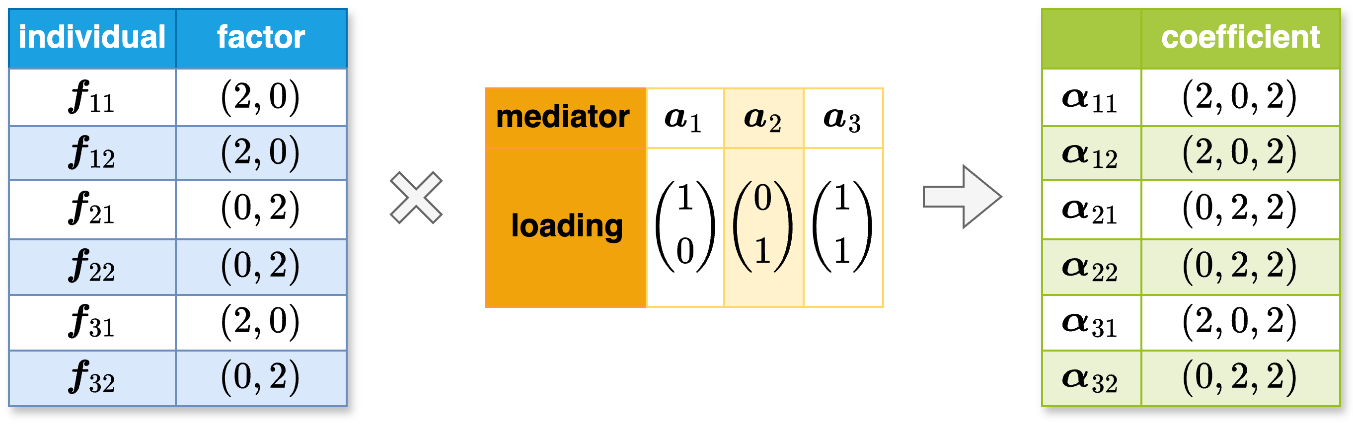
Figure 1: Illustration of the heterogeneous sparsity and subgroup structure when $p=3,n=3,T=2$, and $r=2$.

The $r$-dimensional latent factors could represent $r$ unobserved characteristics (e.g., chromosomal instability) and the coefficient loadings of mediator $k$ could be interpreted as the corresponding scores on these latent factors. A higher concordance between the individual factor and the mediator loading in the $r^{\prime}$th factor indicates that the $k$th mediator is more important for the $i$th individual towards the $r^{\prime}$th dimension for $r^{\prime}=1,\ldots,r$. Given that individual heterogeneity may vary across different latent factors, and the factor loadings of different mediators may also vary, our proposed model allows for heterogeneous mechanisms across different mediators.

For a better illustration, let’s consider a simple case with $3$ mediators, $3$ individuals (each with $2$ measurements), and $2$ latent factors. Figure 1 displays the coefficient loadings ${\boldsymbol{A}}\in\mathbb{R}^{p\times r}$ and the factor matrix $\boldsymbol{F}\in\mathbb{R}^{nT\times r}$. Note that the three individuals all belong to the same subgroup based on the third mediator, while there is no such alignment along the first two mediators. Additionally, we observe dynamic behavior for the third individual, whereas the first two individuals exhibit static characteristics. Hence, our model exhibits greater flexibility compared to existing methods assuming the same heterogeneous structure across all mediators.

The proposed disentanglement also provides additional advantages in imposing structural assumptions across the temporal and mediator dimensions. Denote the dynamic factor matrix for the $i$th individual as $\bar{\boldsymbol{f}}_{i}=({\boldsymbol{f}}_{i1},\ldots,{\boldsymbol{f}}_{iT})^{\top}\in\mathbb{R}^{T\times r}$. We now assume:

1. sparsity pursuit for mediators: $\|\boldsymbol{B}\|_{2,0}\leq s_{b}$; and

2. adjacent homogeneity pursuit for latent factors:

   $$\{\bar{\boldsymbol{f}}_{i}\}_{i=1}^{n}\in\left\{\bar{\boldsymbol{f}}_{i}\in\mathbb{R}^{T\times r}\left|\|D_{f}\operatorname{Vec}({\bar{\boldsymbol{f}}_{i}}^{\top})\|_{0}\leq s_{f}\right.\right\},$$

   where $\operatorname{Vec}({\bar{\boldsymbol{f}}}^{\top}_{i})=({\boldsymbol{f}}_{i1}^{\top},\ldots,{\boldsymbol{f}}_{iT}^{\top})^{\top}\in\mathbb{R}^{Tr}$ and

   $${D_{f}}=\left(\begin{array}[]{cccccc}-{\boldsymbol{I}}_{r}&{\boldsymbol{I}}_{r}&&&&\\ &-{\boldsymbol{I}}_{r}&{\boldsymbol{I}}_{r}&&&\\ &&&\ldots&&\\ &&&&-{\boldsymbol{I}}_{r}&{\boldsymbol{I}}_{r}\end{array}\right)\in\mathbb{R}^{(T-1)r\times Tr}.$$ (3)

Assumption (a) imposes a sparsity assumption on the mediator coefficient loadings. Assumption (b) is imposed on the individualized dynamic latent factors, allowing us to leverage information across the temporal dimension. Note that when $T=2$ and $r=2$, $D_{f}\operatorname{Vec}({\bar{\boldsymbol{f}}_{i}}^{\top})={\boldsymbol{f}}_{i2}-{\boldsymbol{f}}_{i1}$. The $L_{0}$ penalty term here indeed assumes similarity across adjacent time points. Here the first-order discrete difference operator $D_{f}$ can be substituted with higher-order difference operators to capture higher-order smoothness (Tibshirani, 2014). This structural assumption enables us to further reduce the model’s complexity.

2.3 Estimation

The key ingredient in our estimation procedure is a rotation argument. In short, since our target parameter of interest is the low-rank coefficient matrix, we only need to recover the latent factors and loadings up to a rotation and their product will lead to a reliable estimator for the coefficient matrix. We use nuclear norm penalization to enforce the low-rank structure. Let ${\Theta}=(\mathcal{C},{\mathcal{B}})\in\mathbb{R}^{nT\times(p+1)}$ and further let $({\mathcal{A}}_{\mathcal{I}},\mathcal{C}_{\mathcal{I}},{\Theta}_{\mathcal{I}},\boldsymbol{\mathcal{B}}_{\mathcal{I}})$ denote the sub-matrices of $({\mathcal{A}},\mathcal{C},{\Theta},\boldsymbol{\mathcal{B}})$ with index $i\in\mathcal{I}$, respectively. Define the loss functions ${\mathcal{L}}_{M}({{\mathcal{A}}}_{\mathcal{I}})=\sum_{i\in{\mathcal{I}}}\sum_{t=1}^{T}\left\|{\boldsymbol{M}}_{it}-{\boldsymbol{\alpha}}_{it}X_{it}\right\|_{2}^{2}$, and ${\mathcal{L}}_{Y}({{\Theta}}_{\mathcal{I}})={\mathcal{L}}_{Y}(\mathcal{C}_{\mathcal{I}},{\mathcal{B}}_{\mathcal{I}})=\sum_{i\in{\mathcal{I}}}\sum_{t=1}^{T}\left(Y_{it}-\theta_{it}X_{it}-{\boldsymbol{\beta}}_{it}^{\top}{\boldsymbol{M}}_{it}\right)^{2}$. By imposing the structural assumptions (a) and (b), the optimization problem is formulated as

$$\min_{{\Theta},{{\mathcal{A}}}} {\mathcal{L}}_{Y}({\Theta})+{\mathcal{L}}_{M}({{\mathcal{A}}})$$ (4)

s.t. $$\text{rank}({{\mathcal{A}}})\leq r,\quad\text{rank}({\Theta})\leq r,$$

$$\|D_{f}\operatorname{Vec}({\bar{\boldsymbol{f}}}^{\top}_{i})\|_{0}\leq s_{f}\quad(i=1,\ldots,n),\quad\|{\boldsymbol{B}}\|_{2,0}\leq s_{b}.$$

Here we utilize the dimensionality in model (2) to recover the latent factors $\boldsymbol{F}$ and estimate ${\mathcal{B}}$ in (1). Consequently, we propose to solve (4) in a two-step procedure.

1. obtain $\hat{{\mathcal{A}}}$, $\hat{\boldsymbol{F}}$, and $\hat{\boldsymbol{A}}$ by solving

   $$\min_{{{\mathcal{A}}}}{\mathcal{L}}_{M}({{\mathcal{A}}})\quad\text{ s.t. }\text{rank}({{\mathcal{A}}})\leq r,\|D_{f}\operatorname{Vec}({\bar{\boldsymbol{f}}}^{\top}_{i})\|_{0}\leq s_{f}\quad(i=1,\ldots,n).$$ (5)

2. obtain $\hat{\boldsymbol{{\mathcal{B}}}}=\hat{\boldsymbol{F}}{\hat{\boldsymbol{{B}}}}^{\top}$ and $\hat{{\mathcal{C}}}=\hat{\boldsymbol{F}}\hat{{\boldsymbol{{c}}}}$ by solving

   $$\min_{{\boldsymbol{B}},{\boldsymbol{c}}}{\mathcal{L}}_{Y}(\hat{\boldsymbol{F}}{\boldsymbol{{B}}}^{\top},\hat{\boldsymbol{F}}{\boldsymbol{{c}}})\quad\text{ s.t. }\|{\boldsymbol{B}}\|_{2,0}\leq s_{b}.$$ (6)

Here in (5) and (6), the estimators $(\hat{\boldsymbol{{A}}},\hat{\boldsymbol{{B}}},\hat{\boldsymbol{{F}}})$ estimate the original parameter up to a rotation. However, the final estimators $\hat{{\mathcal{A}}}$ and $\hat{{\mathcal{B}}}$ are still consistent estimators of ${{\mathcal{A}}}$ and ${{\mathcal{B}}}$ respectively, as the rotation parts offset.

2.4 Implementation

In this subsection, we provide implementation strategies and tuning details. The low-rank constraint in (5) leads to a NP-hard optimization problem. One approach is to employ a low-rank factorization, yielding a differentiable objective function amenable to gradient-based optimization methods like conjugate gradient and augmented Lagrangian algorithms. However, due to nonconvex constraints, only local minimization is guaranteed (Burer and Monteiro, 2005). To address this, we opt for nuclear norm penalization, the tightest convex relaxation of the NP-hard rank minimization problem (Candes and Plan, 2010). We first obtain an initial estimator $\tilde{{\mathcal{A}}}$ by

$$\min_{{\mathcal{A}}}\quad{\mathcal{L}}_{M}({{\mathcal{A}}})+\lambda_{r}\|{{\mathcal{A}}}\|_{*},$$ (7)

where $\lambda_{r}$ is the regularization parameter. Given an initial estimate ${\mathcal{A}}^{(0)}$, we can obtain an initial $\tilde{{\mathcal{A}}}$ by solving (7) via fixed point iteration (Ma et al., 2011)

$${{\mathcal{A}}}^{(k+1)}=S_{\tau\lambda_{r}}({{\mathcal{A}}}^{(k)}-\tau g({{\mathcal{A}}}^{(k)})),$$ (8)

where $g({{\mathcal{A}}}^{(k)})=\frac{\partial{\mathcal{L}}_{M}({{\mathcal{A}}})}{\partial{{\mathcal{A}}}}\mid_{{{\mathcal{A}}}={{\mathcal{A}}}^{(k)}}$. Here the matrix shrinkage operator $S_{\nu}(\cdot)$ is defined as

$$S_{\nu}({W})=U{D}_{\nu}V^{\top},$$

for any $\nu$ ¿0, where ${W}=UD{V}^{\top}$ is the singular value decomposition (SVD) of a matrix ${W}$, and ${D}_{\nu}$ is defined by replacing the diagonal entry ${D}_{ii}$ of $D$ by $(D_{ii}-\nu)\vee 0$. We choose the hyperparameter $\tau=1/\lambda_{\max}(\boldsymbol{H}^{\top}{\boldsymbol{H}})$ as that in (Ma et al., 2011), where $\boldsymbol{H}=\frac{\partial{\mathcal{L}}_{M}({{\mathcal{A}}})}{\partial{(\operatorname{vec}(\mathcal{A})})^{\top}}$.

To incorporate the structural assumptions on the latent factor and loadings, we propose to alternately minimize in $\boldsymbol{A}$ and $\boldsymbol{F}$. We also use sample splitting here for theoretical justification. Specifically, for each $i\in\{1,\ldots,n\}$, we randomly split the data into $\mathcal{I}$ and $\mathcal{I}^{c}$ where $|\mathcal{I}|=\lceil n/2\rceil$ and $\mathcal{I}\cup\mathcal{I}^{c}=\{1,\ldots,n\}\setminus\{i\}$. Let $\tilde{{\mathcal{A}}}_{\mathcal{I}}=\arg\min_{{\mathcal{A}}_{\mathcal{I}}}\mathcal{L}_{M}({\mathcal{A}}_{\mathcal{I}})+\lambda_{r}\|{\mathcal{A}}_{\mathcal{I}}\|_{*}$ and ${U}_{\mathcal{I}}{D}_{\mathcal{I}}{V}_{\mathcal{I}}^{\top}$ be the SVD of $\tilde{{\mathcal{A}}}_{\mathcal{I}}$. Let $\tilde{\boldsymbol{A}}_{\mathcal{I}}={U}_{\mathcal{I}}{D}_{\mathcal{I}}$ and $\tilde{\boldsymbol{F}}_{\mathcal{I}}={V}_{\mathcal{I}}$. Fixing $\hat{\boldsymbol{A}}_{\mathcal{I}}$, to realize the adjacent homogeneity pursuit (b), we update $\{\bar{\boldsymbol{f}}_{i^{\prime}}\}_{i^{\prime}\in\mathcal{I}^{c}\cup\{i\}}$ by adding a fused SCAD penalty along the temporal dimension, which is a smooth approximation of the $L_{0}$-penalty on $D_{f}\operatorname{Vec}({\bar{\boldsymbol{f}}}^{\top}_{i})$. With a local linear approximation (Zou and Li, 2008) of the SCAD penalty, the optimization in $\boldsymbol{F}$ can be reduced to a generalized lasso problem (Tibshirani and Taylor, 2011). Then we update $\boldsymbol{A}$ and $\boldsymbol{B}$ by fixing $\{\bar{\boldsymbol{f}}_{i^{\prime}}\}_{i^{\prime}\in\mathcal{I}^{c}\cup\{i\}}$. We obtain an estimator for $\boldsymbol{\alpha}_{it}$ and $\boldsymbol{\beta}_{it}$ as $\hat{\boldsymbol{\alpha}}_{it,\mathcal{I}}={\hat{\boldsymbol{A}}_{\mathcal{I}}}{\hat{\boldsymbol{f}}_{it,\mathcal{I}}}$ and $\hat{\boldsymbol{\beta}}_{it,\mathcal{I}}={\hat{\boldsymbol{B}}_{\mathcal{I}}}{\hat{\boldsymbol{f}}_{it,\mathcal{I}}}$, respectively. Finally, we exchange the role of $\mathcal{I}$ and $\mathcal{I}^{c}$ to obtain alternative estimators $\hat{\boldsymbol{\alpha}}_{it,\mathcal{I}^{c}}$ and $\hat{\boldsymbol{\beta}}_{it,\mathcal{I}^{c}}$. The final estimators are obtained by taking an average to fully utilize the sample.

We will show that a one-step update is sufficient for obtaining an accurate estimator for ${\mathcal{A}}$ and can automatically remove the regularization bias from nuclear norm regularization. The above algorithm can be summarized in Algorithm 1. Here $p_{\operatorname{SCAD},\lambda}(\cdot)$ is the SCAD penalty with regularization parameter $\lambda$.

Algorithm 1 Individualized Dynamic Mediation Analysis (IDMA)

1:regularization parameter $(\lambda_{r},\lambda_{b},\lambda_{f})$, and tolerance $\epsilon$, individual index $i$. 1: Randomly split $[n]\setminus\{i\}$ as $\mathcal{I}\cup{\mathcal{I}}^{c}$. 2: Obtain $\tilde{{\mathcal{A}}}_{\mathcal{I}}$ by fixed point iteration in (8) until $|{\mathcal{L}}_{M}({{\mathcal{A}}}_{\mathcal{I}}^{(k)})-{\mathcal{L}}_{M}({{\mathcal{A}}}_{\mathcal{I}}^{(k-1)}))|<\epsilon$. Decompose $\tilde{{\mathcal{A}}}_{\mathcal{I}}=U_{\mathcal{I}}D_{\mathcal{I}}V_{\mathcal{I}}^{\top}$ and let $\tilde{\boldsymbol{A}}_{\mathcal{I}}=U_{\mathcal{I}}D_{\mathcal{I}}$ and $\tilde{\boldsymbol{F}}_{\mathcal{I}}=V_{\mathcal{I}}$. 3: For $i\in\mathcal{I}^{c}\cup\{i\}$, obtain

$$\{\hat{\boldsymbol{f}}_{i^{\prime}t,\mathcal{I}}\}_{t=1}^{T}=\arg\min_{\bar{\boldsymbol{f}}_{i^{\prime}}}\left\{\sum_{t=1}^{T}\left\|{\boldsymbol{M}}_{i^{\prime}t}-\tilde{\boldsymbol{A}}_{\mathcal{I}}{\boldsymbol{f}}_{i^{\prime}t}X_{i^{\prime}t}\right\|_{2}^{2}+\sum_{t=2}^{T}\sum_{r^{\prime}=1}^{r}p_{\operatorname{SCAD},\lambda_{f}}({{f}}_{i^{\prime}tr^{\prime}}-{{f}}_{{i^{\prime},t-1,r^{\prime}}})\right\}.$$

4: Fix $\{{\hat{\boldsymbol{f}}}_{i^{\prime}t,\mathcal{I}}\}_{i^{\prime}\in\mathcal{I}^{c}\cup\{i\}}$, obtain $\hat{\boldsymbol{A}}_{\mathcal{I}}$ by $\hat{\boldsymbol{A}}_{\mathcal{I}}=\arg\min_{\boldsymbol{A}}\mathcal{L}_{M}(\hat{\boldsymbol{F}}_{\mathcal{I}^{c}\cup\{i\}}{\boldsymbol{A}}^{\top}\})$. 5: Fix $\{{\hat{\boldsymbol{f}}}_{i^{\prime}t,\mathcal{I}}\}_{i^{\prime}\in\mathcal{I}^{c}\cup\{i\}}$, obtain $\{\hat{\boldsymbol{B}}_{\mathcal{I}},\hat{\boldsymbol{c}}_{\mathcal{I}}\}$ by optimizing

$$\arg\min_{{\boldsymbol{B}},{\boldsymbol{c}}}\left\{\mathcal{L}_{Y}(\hat{\boldsymbol{F}}_{\mathcal{I}^{c}\cup\{i\}}{\boldsymbol{c}},\hat{\boldsymbol{F}}_{\mathcal{I}^{c}\cup\{i\}}{\boldsymbol{B}}^{\top})+\sum_{k=1}^{p}p_{\operatorname{SCAD},\lambda_{b}}(\|{\boldsymbol{b}}_{k}\|_{2})\right\}.$$ (9)

6: Obtain $\hat{\boldsymbol{\alpha}}_{it,\mathcal{I}}={\hat{\boldsymbol{A}}_{\mathcal{I}}}{\hat{\boldsymbol{f}}_{it,\mathcal{I}}}$ and $\hat{\boldsymbol{\beta}}_{it,\mathcal{I}}={\hat{\boldsymbol{B}}_{\mathcal{I}}}{\hat{\boldsymbol{f}}_{it,\mathcal{I}}}$. 7: Exchange the role of $\mathcal{I}$ and $\mathcal{I}^{c}$, repeat steps 1-5 to obtain $\hat{\boldsymbol{\alpha}}_{it,\mathcal{I}^{c}}$ and $\hat{\boldsymbol{\beta}}_{it,\mathcal{I}^{c}}$.

2:$\hat{\boldsymbol{\alpha}}_{it}=(\hat{\boldsymbol{\alpha}}_{it,\mathcal{I}}+\hat{\boldsymbol{\alpha}}_{it,\mathcal{I}^{c}})/2$ and $\hat{\boldsymbol{\beta}}_{it}=(\hat{\boldsymbol{\beta}}_{it,\mathcal{I}}+\hat{\boldsymbol{\beta}}_{it,\mathcal{I}^{c}})/2$.

In practice, sample splitting may lead to less satisfactory finite-sample results even if they enjoy good asymptotic properties. Recently, Choi et al. (2024) have proven that the low-rank estimation procedure without sample splitting is asymptotically equivalent to the auxiliary leave-one-out estimation, which enjoys a similar effect to sample splitting by separating out the correlated part. Therefore, in our implementation we use the whole sample to estimate the latent factors and the loadings. The sample-splitting procedure listed above is only for theoretical consideration.

To incorporate the homogeneous and subgroup-based models, we also modify Step 3 by applying K-means clustering to the estimated factors $\{\operatorname{Vec}(\{\hat{\boldsymbol{f}}_{it}\}_{t=1}^{T})\}_{i=1}^{n}$ to obtain $c_{f}$ subgroups, where $c_{f}$ is a tuning parameter. One can also consider clustering separately at each time point for more flexible modelling.

In the following, we discuss the choice of tuning parameters. We assume that $r$ is known, for simplicity. In fact, the rank $r$ can be consistently estimated under the spiked singular value assumption; see, for example, Fan et al. (2022). Denote $\tilde{\boldsymbol{X}}={\boldsymbol{X}}\otimes{\boldsymbol{1}}_{p}^{\top}$ where $\boldsymbol{X}\in\mathbb{R}^{nT}$ and $\boldsymbol{X}_{T(i-1)+t}=X_{it}$. In the nuclear norm penalization step, we set $\lambda_{r}=2.2\bar{Q}(\|\boldsymbol{\Delta}\circ\tilde{\boldsymbol{X}}\|;0.95)$ as suggested in Chernozhukov et al. (2018), where $\bar{Q}(W;q)$ denotes the $q$ th quantile of a random variable $W$ and $\boldsymbol{\Delta}$ is an $nT\times p$ matrix whose elements $\Delta_{i,k}$ are generated as $\mathcal{N}\left(0,\widehat{\sigma}_{e}^{2}\right)$ independent across $(i,k)$ for some estimated $\widehat{\sigma}_{e}^{2}$. The regularization parameter $\lambda_{b}$ to induce row-sparsity of $\boldsymbol{B}$ is selected by 5-fold cross validation. To remove noises in practice, we also shrink $\hat{\boldsymbol{b}}_{k}$ to 0 if $\|\hat{\boldsymbol{b}}_{k}\|_{2}<\hat{\boldsymbol{\mu}}_{b}+0.5\hat{{\sigma}}_{b}$, where $\hat{\boldsymbol{\mu}}_{b}$ and $\hat{{\sigma}}_{b}$ are the mean and standard error of $\{\|\hat{\boldsymbol{b}}_{k}\|_{2}\}_{k=1}^{p}$, respectively. To automatically group individuals, we propose a modified BIC (Park et al., 2022) to select the number of subgroups $c_{f}$ as well as the fusion regularization parameter $\lambda_{f}$. Let $\operatorname{df}^{B}_{\lambda_{f},c_{f}}$ be the number of the row-support of $\hat{{\boldsymbol{B}}}$ and $\operatorname{df}^{F}_{\lambda_{f},c_{f}}$ be the number of distinct rows of $\hat{{\boldsymbol{F}}}$. We use

$$\operatorname{BIC}(\lambda_{f},c_{f})=\log\left(\frac{{\mathcal{L}}_{M}(\hat{{\mathcal{A}}}_{\lambda_{f},c_{f}})}{nT}\right)+\log\left(\frac{{\mathcal{L}}_{Y}(\hat{\boldsymbol{{\Theta}}}_{\lambda_{f},c_{f}})}{nT}\right)+c_{N}r\operatorname{df}^{F}_{\lambda_{f},c_{f}}+d_{N}r\operatorname{df}^{B}_{\lambda_{f},c_{f}}$$ (10)

where $N=nT$ is the number of total observations, $c_{N}=C_{1}\log\log(nT)\log p/(nT)$, and $d_{N}=C_{2}\log\log(nT)/(nT)$. In the simulation, we set $C_{1}=0.5$ and $C_{2}=0.5$.

3 Theoretical Properties

In this section, we investigate the asymptotic properties of our IDMA estimator. Here we consider a more general case where $\beta_{itk}={\boldsymbol{b}}_{k}^{\top}{\boldsymbol{g}}_{it}$ and ${\boldsymbol{g}}_{it}$=${\boldsymbol{C}}{\boldsymbol{f}}_{it}$ for some invertible matrix ${\boldsymbol{C}}\in\mathbb{R}^{r\times r}$; that is, ${\boldsymbol{g}}_{it}$ is a rotation of ${\boldsymbol{f}}_{it}$. Therefore, $\mathcal{B}=\boldsymbol{G}\boldsymbol{B}^{\top}$ with ${\boldsymbol{G}}={\boldsymbol{F}}{\boldsymbol{C}}^{\top}$. Utilizing the singular value decomposition (SVD) ${\mathcal{A}}={{U}}_{A}{{D}}_{A}{{V}}_{A}$ and ${\mathcal{B}}={{U}}_{B}{{D}}_{B}{{V}}_{B}$, we define $\boldsymbol{F}={U}_{A}{D}_{A}$, $\boldsymbol{A}={V}_{A}$, $\boldsymbol{G}={U}_{B}{D}_{B}$, and $\boldsymbol{B}={V}_{B}$. In the special case where $\boldsymbol{C}$ is an identity matrix, it aligns with the assumption outlined in Section 2. In practice, the underlying mechanisms of factors between $\boldsymbol{M}$ and $Y$ and between $X$ and $\boldsymbol{M}$ may differ. Therefore, the rotation structure serves as a relaxation, enhancing the flexibility of our model. Moreover, since $\boldsymbol{C}$ is invertible, we have $\|{\boldsymbol{B}}\|_{2,0}=\|{\boldsymbol{B}}\boldsymbol{C}\|_{2,0}$, preserving the estimation procedure outlined in Section 2.4.

Let $\hat{\mathcal{A}}=\{\hat{\boldsymbol{\alpha}}_{it}\}_{1:n,1:T}$ and $\hat{\mathcal{B}}=\{\hat{\boldsymbol{\beta}}_{it}\}_{1:n,1:T}$. We assume that the parameter space for ${\bar{\boldsymbol{f}}_{i}}$ is

$$\mathcal{M}_{\boldsymbol{f}}^{(i)}=\left\{\bar{\boldsymbol{f}}_{i}\in\mathbb{R}^{T\times r}:{{f}}_{i,t-1,r^{\prime}}={{f}}_{i,t,r^{\prime}},\text{ for }t\in\mathcal{T}^{(i)}_{l},r^{\prime}=1,\ldots,r,l=1,\ldots,L\right\},$$

where $\cup_{l=1}^{L}\mathcal{T}^{(i)}_{l}=[T]$. Without loss of generality, we assume that $\mathcal{T}^{(i)}_{l}$ does not depend on $r^{\prime}$ for notational simplicity. Let $\boldsymbol{\mu}_{i}\in\mathbb{R}^{L\times r}=[\boldsymbol{\mu}_{i1},\ldots,\boldsymbol{\mu}_{iL}]^{\top}$ denote the partitioned factor matrix, where the $l$th row represents a factor in the $l$th group. Let $Q_{i}\in\mathbb{R}^{T\times L}$ denote the indicator matrix, where $Q_{i}(t,l)=1$ represents $t\in\mathcal{T}_{l}$ for the $i$th individual and 0 otherwise. Then we have $\boldsymbol{f}_{i}=Q_{i}\boldsymbol{\mu}_{i}$ $(i=1,\ldots,n).$ Denote $\bar{\boldsymbol{f}}_{i,\mathcal{I}}^{(0)}=(\hat{\boldsymbol{f}}_{i1,\mathcal{I}},\ldots,\hat{\boldsymbol{f}}_{iT,\mathcal{I}})^{\top}$. Let $\hat{\boldsymbol{\mu}}_{i,\mathcal{I}}=[\hat{\boldsymbol{\mu}}_{i1,\mathcal{I}},\ldots,\hat{\boldsymbol{\mu}}_{iL,\mathcal{I}}]^{\top}$ be the distinct rows $\bar{\boldsymbol{f}}_{i,\mathcal{I}}^{(0)}$ and consider the oracle estimator of $\boldsymbol{\mu}_{i}$ when the partition $\{\mathcal{T}^{(i)}_{l}\}_{l=1}^{L}$ is known. Let ${\boldsymbol{\alpha}}^{\mathrm{g}}_{il}={\boldsymbol{A}}{\boldsymbol{\mu}}_{{i}l}$ , $\hat{{\boldsymbol{\alpha}}}^{\mathrm{g}}_{il,\mathcal{I}}=\hat{\boldsymbol{A}}_{\mathcal{I}}\hat{\boldsymbol{\mu}}_{il,\mathcal{I}}$, and $\hat{{\boldsymbol{\alpha}}}^{\mathrm{g}}_{il}=(\hat{{\boldsymbol{\alpha}}}^{\mathrm{g}}_{il,\mathcal{I}}+\hat{{\boldsymbol{\alpha}}}^{\mathrm{g}}_{il,\mathcal{I}^{c}})/2$. Here “$\mathrm{g}$” is short for “$\mathrm{group}$”. In fact, one can show that the adaptive estimators under unknown partitions will converge to the oracle estimators under regular assumptions. For notational simplicity, we do not consider the case here. Let $U_{A}=\left[{\boldsymbol{u}}_{11},\ldots,{\boldsymbol{u}}_{nT}\right]^{\prime}$ and $V_{A}=\left[{\boldsymbol{v}}_{1},\ldots,{\boldsymbol{v}}_{p}\right]^{\prime}$ denote the $nT\times r$ and $p\times$ $r$ matrices which represent the left singular vectors and right singular vectors of $\mathcal{A}$, respectively, corresponding to the nonzero singular values. We provide the following key assumptions.

Assumption 2 (Spiked singular value)

$\mathcal{A}$ is a rank $r$ matrix where $r=O(1)$. In addition, the nonzero singular values of $\mathcal{A}$ are ”spiked”:

$$\psi_{1}\left(\mathcal{A}\right)\geq\cdots\geq\psi_{r}\left(\mathcal{A}\right)\geq\psi_{np},\quad\psi_{j}\left(\mathcal{A}\right)=0,\text{ for any }j>r$$

for some sequence $\psi_{np}$ satisfying $((nT)\vee p)^{3/4}=o(\psi_{np})$. Further assume that $\kappa=\psi_{1}(\mathcal{A})/\psi_{r}(\mathcal{A})=O(1).$

Assumption 2 here requires that the nonzero singular values are large enough to ensure the consistent estimation of the rank and accurate estimation of the singular vectors. This is necessary to establish entriwise convergence properties for the low-rank matrix.

Assumption 3 (Incoherent singular vectors)

We assume incoherent singular-vectors:

$$\mathbb{E}\max_{j\leq p}\left\|{\boldsymbol{v}}_{j}\right\|^{2}=O\left({rp^{-1}}\right),\quad\mathbb{E}\max_{i\leq n}\max_{t\leq T}\left\|{\boldsymbol{u}}_{it}\right\|^{2}=O\left({r{(nT)}^{-1}}\right).$$

Assumption 3 prevents the information of the row and column spaces of the matrix from being too concentrated in a few rows or columns, which is known to be crucial for reliable recovery of low-rank matrices (Candes and Plan, 2010; Chen, 2015; Chen et al., 2020).

For a matrix $W$ with singular value decomposition $W=U_{W}D_{W}V_{W}$, let $P_{W}(\Delta)=U_{W}U_{W}^{\top}\Delta V_{W}V_{W}^{\top}$ and $P_{W}^{\perp}(\Delta)=\Delta-P_{W}(\Delta)$. Define the restricted set $\mathcal{R}^{W}_{a}=\{\Delta:\left\|P_{W}(\Delta)\right\|_{*}\leq a\left\|P_{W}^{\perp}(\Delta)\right\|_{*}\}$. Recall that $\tilde{\boldsymbol{X}}={\boldsymbol{X}}\otimes{\boldsymbol{1}}_{p}^{\top}$ where $\boldsymbol{X}\in\mathbb{R}^{nT}$ and $\boldsymbol{X}_{T(i-1)+t}=X_{it}$.

Assumption 4 (Restricted Strong Convexity)

For any $a>0$, there exists a constant $\kappa_{a}$, such that $\|\tilde{\boldsymbol{X}}\odot\Delta\|_{F}^{2}\geq\kappa_{a}\|\Delta\|_{F}^{2},\text{ for any }\Delta\in\mathcal{R}_{a}^{\mathcal{A}}$. The same also holds when $\mathcal{A}$ is replaced by $\mathcal{A}_{\mathcal{I}}$ or $\mathcal{A}_{\mathcal{I}^{c}}$.

The restricted strong convexity condition is commonly employed in regularized estimation. See Negahban et al. (2012).

Theorem 1

Under Assumptions 1 - 4, LABEL:assump:error(i) and LABEL:assump:moment in Section LABEL:subsec:assump of the Supplementary Materials, if $\lambda_{r}\asymp\sqrt{nT+p}$, then for fixed $i\leq n$, fixed $j\leq p$, and fixed $l\leq L$, we have

$$\left|\hat{\alpha}^{\mathrm{g}}_{ilj}-{\alpha}^{\mathrm{g}}_{ilj}\right|=O_{p}\left({{(nT)}}^{-1/2}+(p|\mathcal{T}_{l}^{(i)}|)^{-1/2}\right).$$

Let ${\boldsymbol{\beta}}^{\mathrm{g}}_{il}={\boldsymbol{B}}{\boldsymbol{\mu}}_{{i}l}$ and $\hat{\boldsymbol{\beta}}^{\mathrm{g}}_{il,\mathcal{I}}=\hat{\boldsymbol{B}}_{\mathcal{I}}\hat{\boldsymbol{\mu}}_{il,\mathcal{I}}$ for some index set $\mathcal{I}$. Let $\hat{\boldsymbol{\beta}}^{\mathrm{g}}_{il,\mathcal{I}}=(\hat{\boldsymbol{\beta}}^{\mathrm{g}}_{il,\mathcal{I}}+\hat{\boldsymbol{\beta}}^{\mathrm{g}}_{il,\mathcal{I}^{c}})/2$. Further denote the support of nonzero columns in $\mathcal{B}$ and $\hat{\mathcal{B}}$ as $\mathcal{S}$ and $\hat{\mathcal{S}}$ respectively.

Theorem 2

Under Assumptions 1 - 4, LABEL:assump:error(ii) and LABEL:assump:moment in Section LABEL:subsec:assump of the Supplementary Materials, if $\lambda_{r}\asymp\sqrt{nT+p}$ , $\lambda_{b}\rightarrow 0$, and $\sqrt{nT}\lambda_{b}\rightarrow\infty$, then for fixed $i\leq n$ and $l\leq L$, we have

(i) $\hat{\beta}^{\mathrm{g}}_{ilj}=0$, for $j=s+1,\ldots,p$, with probability approaching 1. Consequently, $\mathcal{P}({\mathcal{S}}\subset\hat{\mathcal{S}})\rightarrow 1$.

(ii) $|\hat{\beta}^{\mathrm{g}}_{ilj}-{\beta}^{\mathrm{g}}_{ilj}|=O_{p}((nT)^{-1/2}+(p|\mathcal{T}_{l}^{(i)}|)^{-1/2})$.

Theorem 1 and Theorem 2 establish the individual-wise convergence rates for the dynamic mediation coefficients $\boldsymbol{\alpha}_{it}$ and $\boldsymbol{\beta}_{it}$, respectively. Moreover, Theorem 2 demonstrates that we can reliably recover the significant mediators in the outcome model. Combined with Theorem 1, we can consistently detect mediators with significant mediation effects.

4 Simulation

In the simulation, we evaluate three candidate mediation analysis methods. The first two are the method proposed in Zhang et al. (2016) implemented with “MCP” and “SCAD” penalties respectively. Additionally, we consider the debiased-lasso based method proposed in Perera et al. (2022). We also compare the performance of the subgroup-based heterogeneous mediation method proposed by Xue et al. (2022). Since these methods are not designed for longitudinal data, we fit each model using the data at each time point separately.

For each method, we use $\sqrt{\|\hat{\mathcal{A}}\odot\hat{\mathcal{B}}-{\mathcal{A}}\odot{\mathcal{B}}\|_{F}^{2}/(nTp)}$ to evaluate the root mean square error (RMSE). To evaluate the dynamic patterns captured by each estimator, we first define a soft trend operator $\mathbf{T}$ for a sequence $\boldsymbol{h}\in\mathbb{R}^{T}$ as $\mathbf{T}({\boldsymbol{h}})=\boldsymbol{d}\in\mathbb{R}^{T-1},$ where $d_{j}={I}(h_{j+1}-h_{j}>c)+(-1){I}(h_{j+1}-h_{j}<-c)$ $(j=1,\ldots,T-1)$ and some threshold $c$. The operator $\boldsymbol{T}$ transforms a continuous sequence to its corresponding trend vector. Here we choose $c$ as $0.1$ instead of $0$ to allow for slight disturbances over time. Let $\hat{\boldsymbol{\gamma}}_{i\cdot k}$ =$(\hat{{\alpha}}_{i1k}\hat{{\beta}}_{i1k},\ldots,\hat{{\alpha}}_{iTk}\hat{{\beta}}_{iTk})^{\top}$ be the coefficient estimators for the $i$th individual on the $k$th mediator. Define the true parameters ${\boldsymbol{\gamma}}_{i\cdot k}$ in the same way. Then we define the matching error (ME) for each estimator as $\operatorname{ME}=\sqrt{{\sum_{i=1}^{n}\sum_{k=1}^{p}\|\mathbf{T}(\hat{\boldsymbol{\gamma}}_{i\cdot k})-\mathbf{T}({\boldsymbol{\gamma}}_{i\cdot k})\|^{2}}/{(np(T-1)})}$. Let ${\gamma}_{itk}={\alpha}_{itk}{\beta}_{itk}$ and $\hat{\gamma}_{itk}=\hat{\alpha}_{itk}\hat{\beta}_{itk}$. To evaluate selection accuracy on the individual level, we use the false negative ratio and false positive ratio over all parameters as follows

$$\mathrm{FN.all}=\frac{\sum_{i=1}^{n}\sum_{t=1}^{T}\sum_{k=1}^{p}I\left(\hat{\gamma}_{itk}=0,{\gamma}_{itk}\neq 0\right)}{\sum_{i=1}^{n}\sum_{t=1}^{T}\sum_{k=1}^{p}I\left({\gamma}_{itk}\neq 0\right)},\quad\mathrm{FP.all}=\frac{\sum_{i=1}^{n}\sum_{t=1}^{T}\sum_{k=1}^{p}I\left(\hat{\gamma}_{itk}\neq 0,{\gamma}_{itk}=0\right)}{\sum_{i=1}^{n}\sum_{t=1}^{T}\sum_{k=1}^{p}I\left({\gamma}_{itk}=0\right)}.$$

Let $w_{k}=\sum_{i=1}^{n}\sum_{t=1}^{T}|{\gamma}_{itk}|$ and $\hat{w}_{k}=\sum_{i=1}^{n}\sum_{t=1}^{T}|\hat{\gamma}_{itk}|$. We also evaluate the selection accuracy on the population level by the averaged false negative ratio and false positive ratio

$$\mathrm{FN.avg}=\frac{\sum_{k=1}^{p}I\left(\hat{w}_{k}=0,w_{k}\neq 0\right)}{\sum_{k=1}^{p}I\left(w_{k}\neq 0\right)},\quad\mathrm{FP.avg}=\frac{\sum_{k=1}^{p}I\left(\hat{w}_{k}\neq 0,w_{k}=0\right)}{\sum_{k=1}^{p}I\left(w_{k}=0\right)}.$$

We explore three distinct settings. Setting 1 represents a heterogeneous scenario where both positive and negative individual effects exist, which offset each other at the population level. This heterogeneous setting plays a pivotal role in achieving more comprehensive diagnostic coverage of Alzheimer’s disease, forming a basis for implementing precision medicine approaches (Jellinger, 2022). Additionally, we assess the adaptivity of our method in a homogeneous setting, denoted as Setting 2, where all individuals share the same dynamic mediation effects. In Section LABEL:sec:addsimu of the Supplementary Materials, we also examine another heterogeneous setting with no counteractive effects (Setting 3). Across all settings, we set the number of time points as $T=5$ and generate the exposure $X_{it}$ from $\operatorname{Unif}[1,2]$. We consider $n=(50,100)$ and $p=(30,100)$. For hyper-parameter selection, we set $\lambda_{r}$ as mentioned in Section 2.4 and select $(\lambda_{r},c_{f})$ by minimizing the BIC in (10).

4.1 Heterogeneous setting with counteractive effects

We first investigate the performance of all methods in a heterogeneous setting, where there are individually significant but collectively non-significant effects at the population level. Here we set $r=2$ and $\boldsymbol{c}=(1,0)^{\top}$. Let $\bar{\boldsymbol{f}}_{i}^{(r^{\prime})}=(f_{i1r^{\prime}},\ldots,f_{iTr^{\prime}})^{\top}$ denote the $r^{\prime}$th column of $\bar{\boldsymbol{f}}_{i}$. For $i=1,\ldots,n$, we first generate ${\mu}_{i1},{\mu}_{i2}$ from $\mathcal{N}(1,0.15)$ independently and fix them. Then we set $\bar{\boldsymbol{f}}_{i}^{(1)}$ as $(\mu_{i1}\mathbf{1}_{2},(\mu_{i1}-0.5)\mathbf{1}_{3})^{\top}$ and $\bar{\boldsymbol{f}}_{i}^{(2)}$ as $w_{i}((\mu_{i2}-0.5)\mathbf{1}_{2},\mu_{i2}\mathbf{1}_{3})^{\top},$ where $w_{i}$’s are independent Radamacher variables. We set ${\boldsymbol{b}}_{k}=(1,0)^{\top}$ for $k=1,3,5,7$; ${\boldsymbol{b}}_{k}=(0,1)^{\top}$ for $k=2,4,6,8$; and ${\boldsymbol{b}}_{k}=(0,0)^{\top}$ for $k=9,\ldots,p$. We also set the proportion of mediators with counteractive effects in the mediator model as $p_{\operatorname{hete}}=30\%$. For $k=1,\ldots,p$, we first generate $w_{k}\sim\operatorname{Bern}(1,p_{\operatorname{hete}}),h_{k}\sim\operatorname{Bern}(1,0.5),\mu_{k}\sim h_{k}\mathcal{N}(1.5,0.5)+(1-h_{k})\mathcal{N}(-1.5,0.5)$, and then set ${\boldsymbol{a}}_{k}=(1-w_{k})(\mu_{k},0)^{\top}+w_{k}(0,\mu_{k})^{\top}$. Since $\alpha_{itk}={\boldsymbol{a}}_{k}^{\top}{\boldsymbol{f}}_{it}$, $\beta_{itk}={\boldsymbol{b}}_{k}^{\top}{\boldsymbol{f}}_{it}$, and $E[\bar{\boldsymbol{f}}_{i}^{(2)}]=0$, mediators with loadings ${\boldsymbol{a}}_{k}=(0,\mu_{k})^{\top}$ (corresponding to $w_{k}=1$) and ${\boldsymbol{b}}_{k}=(0,1)^{\top}$ have counteractive effects on the population level. Therefore, it is difficult to detect them using a homogeneous model.

The random error vectors $\operatorname{Vec}(\{\Delta_{it}\}_{t=1}^{T})$ are generated from two components ${\boldsymbol{\xi}}^{(1)}_{i}\in{\mathbb{R}}^{p}\sim\mathcal{N}({\boldsymbol{0}}_{p},\Sigma^{M})$ and ${\boldsymbol{\xi}}_{i}^{(2)}\in{\mathbb{R}}^{T}\sim\mathcal{N}({\boldsymbol{0}}_{T},\Sigma^{T})$, where $\Sigma^{M}_{k,k^{\prime}}={0.3}^{|k-k^{\prime}|}$ and $\Sigma^{T}_{t,t^{\prime}}=0.7\times{0.2}^{|t-t^{\prime}|}$. We let $\operatorname{Vec}(\{\Delta_{it}\}_{t=1}^{T})={\mathbf{1}}_{T}\otimes{\boldsymbol{\xi}}_{i}^{(1)}+{\boldsymbol{\xi}}_{i}^{(2)}\otimes{\mathbf{1}}_{p}$. We also generate $\varepsilon_{it}$ from $\mathcal{N}({\boldsymbol{0}}_{T},\Sigma^{T})$. The simulation results are presented in Table 1.

Table 1: Performance of the proposed method and competing methods in the heterogeneous setting with counteractive effects. “IDMA”: our proposed method; “HIMA-MCP”: Zhang et al. (2016) with “MCP” penalty; “HIMA-SCAD”: Zhang et al. (2016) with “SCAD” penalty; “HIMA2”: Perera et al. (2022); “gHIMA”: Xue et al. (2022).

$p$	$n$	Method	RMSE	ME	FN.avg	FP.avg	FN.all	FP.all
30	50	IDMA	0.261(0.077)	0.212(0.074)	0.03(0.067)	0.026(0.035)	0.03(0.067)	0.026(0.035)
		HIMA-MCP	0.796(0.088)	0.513(0.062)	0.369(0.12)	0.429(0.131)	0.723(0.059)	0.116(0.04)
		HIMA-SCAD	0.811(0.101)	0.539(0.072)	0.361(0.119)	0.515(0.137)	0.704(0.064)	0.147(0.05)
		HIMA2	0.838(0.071)	0.901(0.034)	0.001(0.012)	0.999(0.006)	0.147(0.05)	0.872(0.018)
		gHIMA	1.183(0.188)	0.831(0.054)	0(0)	1(0)	0.554(0.055)	0.441(0.056)
	100	IDMA	0.194(0.03)	0.178(0.058)	0.007(0.03)	0.003(0.011)	0.007(0.03)	0.003(0.011)
		HIMA-MCP	0.697(0.038)	0.485(0.054)	0.406(0.086)	0.394(0.119)	0.689(0.053)	0.111(0.037)
		HIMA-SCAD	0.698(0.037)	0.517(0.06)	0.374(0.101)	0.512(0.129)	0.648(0.054)	0.155(0.049)
		HIMA2	0.724(0.036)	0.871(0.032)	0(0)	1(0)	0(0)	1(0)
		gHIMA	0.821(0.047)	0.703(0.047)	0(0)	1(0)	0.694(0.042)	0.297(0.042)
100	50	IDMA	0.106(0.07)	0.072(0.05)	0.021(0.062)	0.029(0.041)	0.021(0.062)	0.029(0.041)
		HIMA-MCP	0.415(0.047)	0.257(0.031)	0.554(0.12)	0.104(0.038)	0.845(0.051)	0.024(0.009)
		HIMA-SCAD	0.416(0.047)	0.269(0.035)	0.52(0.115)	0.13(0.045)	0.83(0.055)	0.03(0.011)
		HIMA2	0.522(0.044)	0.602(0.019)	0.402(0.123)	0.593(0.054)	0.656(0.06)	0.253(0.005)
		gHIMA	0.717(0.066)	0.6(0.026)	0(0)	1(0)	0.79(0.026)	0.206(0.02)
	100	IDMA	0.061(0.009)	0.038(0.023)	0(0)	0.005(0.009)	0(0)	0.005(0.009)
		HIMA-MCP	0.354(0.019)	0.24(0.029)	0.465(0.078)	0.085(0.031)	0.757(0.044)	0.019(0.006)
		HIMA-SCAD	0.351(0.019)	0.234(0.04)	0.449(0.082)	0.107(0.049)	0.747(0.054)	0.024(0.012)
		HIMA2	0.443(0.026)	0.687(0.018)	0.392(0.099)	0.694(0.049)	0.533(0.044)	0.438(0.004)
		gHIMA	0.593(0.044)	0.599(0.033)	0(0)	1(0)	0.784(0.026)	0.215(0.025)

In general, the IDMA outperforms all the other candidates under all measures across different $n$ and $p$. We highlight four points here.

First, the IDMA reduces the RMSE of those homogeneous methods by over 65%, with significantly improved false negative and false positive ratios of both the population and individual levels. It effectively controls both FP.avg and FP.all below level 0.03 when $n=50$ and below level 0.005 when $n=100$, respectively, while maintaining much smaller FN.avg and FN.all. This indicates that the IDMA excels at detecting heterogeneity among individuals and selecting mediators in a personalized manner. In contrast, homogeneous methods only identify significant mediators at a population level, resulting in a high false negative ratio. This is due to the presence of $30\%$ of mediators whose effects offset at the population level despite their significance at the individual level. Detecting these mediators with a homogeneous model proves challenging, even with a large sample size. In contrast, the IDMA retrieves individualized effects through low-rank decomposition, enabling the detection of significant mediators even if their effects offset at the population level.

Second, the IDMA exhibits the smallest ME across all scenarios, indicating its superior ability to capture dynamic patterns of mediation effects. This can be attributed to two factors: the low-rank structure aids in recovering the underlying dynamic latent factors, facilitating the capture of dynamic changes in coefficients; and the fused penalty imposed on dynamic factors further enhances information borrowing from adjacent time points.

Third, the subgroup-based method gHIMA performs even worse than the homogeneous method in the heterogeneous settings. This is due to the absence of a subgroup structure in the examined heterogeneous setting. In contrast, the IDMA effectively captures heterogeneity from the low-rank structure, enhancing its robustness and accommodating various heterogeneous mechanisms.

Last, the performance of the IDMA significantly improves with increased sample size, whereas the improvement in other methods is not as substantial. Particularly in the high-dimensional setting when $p=100$, both the RMSE and ME of the IDMA are reduced by around 50% when the sample size $n$ increases from 50 to 100. In contrast, the decreases in RMSE and ME in the other methods are all less than 14% and 8%, respectively. Moreover, as $n$ increases, the FN’s of the IDMA decrease drastically with FP’s even under a lower level.

4.2 Homogeneous setting

We consider a homogeneous setting to evaluate the robustness of the IDMA. Let $r=2$. We generate ${\boldsymbol{a}}_{k}$ from $w_{k}\times\mathcal{N}((1,0)^{\top},0.1\times{\mathbf{I}}_{2})+(1-w_{k})\times\mathcal{N}((0,1)^{\top},0.1\times{\mathbf{I}}_{2})$ with $w_{k}\sim\operatorname{Bern}(1,0.5)$ for $k=1,\ldots,p$, and fix them. Let $\boldsymbol{c}=(1,0)^{\top}$. For $p=30$, we generate ${\boldsymbol{b}}_{k}$ in the same way as that for ${\boldsymbol{a}}_{k}$ and further set ${\boldsymbol{b}}_{k}=\boldsymbol{0}$ if $\|{\boldsymbol{b}}_{k}\|^{2}_{2}<0.8$. For $p=100$, we set ${\boldsymbol{b}}_{1}={\boldsymbol{b}}_{2}=(1.5,0)^{\top}$, ${\boldsymbol{b}}_{3}={\boldsymbol{b}}_{4}=(0,1.5)^{\top}$, and ${\boldsymbol{b}}_{k}=(0,0)^{\top}$ for $k=5,\ldots,p$. The latent factors for all $i=1,\ldots,n$ are set as ${\boldsymbol{f}}_{it}=(1.5,0.1)^{\top}$ for $t=1,2,3$ and ${\boldsymbol{f}}_{it}=(0.1,1.5)^{\top}$ for $t=4,5$. The $\epsilon_{it}$’s are the same as those in Section 4.1, while the $\boldsymbol{\delta}_{it}$’s are generated with $\Sigma^{M}$ and $\Sigma^{T}$ replaced by $\Sigma^{M}_{k,k^{\prime}}=0.5\times{0.3}^{|k-k^{\prime}|}$ and $\Sigma^{T}_{t,t^{\prime}}=0.5\times{0.2}^{|t-t^{\prime}|}$, respectively. The results of all the candidate methods are presented in Table 2.

Table 2: Performance of the proposed method and competing methods in the homogeneous setting. “IDMA”: our proposed method; “HIMA-MCP”: Zhang et al. (2016) with “MCP” penalty; “HIMA-SCAD”: Zhang et al. (2016) with “SCAD” penalty; “HIMA2”: Perera et al. (2022); “gHIMA”: Xue et al. (2022).

$p$	$n$	Method	RMSE	ME	FN.avg	FP.avg	FN.all	FP.all
30	50	IDMA	0.126(0.026)	0.285(0.079)	0(0)	0(0)	0(0)	0(0)
		HIMA-MCP	0.649(0.112)	0.577(0.056)	0(0)	0.412(0.137)	0.3(0.068)	0.115(0.046)
		HIMA-SCAD	0.649(0.113)	0.574(0.065)	0(0)	0.443(0.166)	0.301(0.07)	0.128(0.06)
		HIMA2	0.675(0.09)	0.855(0.042)	0(0)	1(0.005)	0.11(0.038)	0.858(0.014)
		gHIMA	0.92(0.086)	0.535(0.047)	0(0)	1(0)	0.835(0.036)	0.184(0.035)
	100	IDMA	0.097(0.017)	0.262(0.074)	0(0)	0(0)	0(0)	0(0)
		HIMA-MCP	0.363(0.067)	0.489(0.043)	0(0)	0.211(0.115)	0.14(0.027)	0.048(0.029)
		HIMA-SCAD	0.363(0.068)	0.478(0.045)	0(0)	0.207(0.139)	0.148(0.03)	0.046(0.033)
		HIMA2	0.371(0.065)	0.689(0.042)	0(0)	1(0)	0(0)	1(0)
		gHIMA	0.84(0.049)	0.529(0.031)	0(0)	1(0)	0.804(0.027)	0.191(0.027)
100	50	IDMA	0.066(0.013)	0.126(0.033)	0(0)	0.004(0.008)	0(0)	0.004(0.008)
		HIMA-MCP	0.22(0.061)	0.244(0.036)	0(0)	0.107(0.04)	0.398(0.063)	0.024(0.01)
		HIMA-SCAD	0.219(0.061)	0.228(0.04)	0(0)	0.104(0.054)	0.416(0.062)	0.023(0.012)
		HIMA2	0.423(0.079)	0.582(0.019)	0.015(0.06)	0.679(0.035)	0.488(0.079)	0.25(0.003)
		gHIMA	0.547(0.101)	0.148(0.038)	0.155(0.279)	0.714(0.423)	0.842(0.119)	0.008(0.007)
	100	IDMA	0.049(0.012)	0.11(0.035)	0(0)	0.002(0.005)	0(0)	0.002(0.005)
		HIMA-MCP	0.154(0.039)	0.219(0.036)	0(0)	0.093(0.049)	0.321(0.067)	0.02(0.011)
		HIMA-SCAD	0.154(0.04)	0.185(0.033)	0(0)	0.06(0.045)	0.37(0.074)	0.013(0.01)
		HIMA2	0.311(0.043)	0.654(0.028)	0(0)	0.908(0.024)	0.374(0.069)	0.432(0.003)
		gHIMA	0.479(0.067)	0.128(0.029)	0.227(0.302)	0.62(0.488)	0.812(0.086)	0.004(0.005)

As evident from Table 2, the IDMA demonstrates robustness in the homogeneous setting and exhibits the best performance among all candidates across different $n$ and $p$. Robustness is particularly crucial in practical scenarios, as we are often uncertain about the degree of heterogeneity among individuals. The notable improvement over existing methods is attributed to the utilization of the low-rank structure in estimating the mediator model (2). This enables us to leverage the correlation structure among mediators from the same individual to generate more accurate estimates of $\boldsymbol{\alpha}_{it}$. Furthermore, the fusion penalty allows for information borrowing from adjacent time points. Additionally, we observe that the performance of IDMA further enhances with increased sample size. Specifically, the RMSE of IDMA decreases by 25% when the sample size is doubled from 50 to 100.

5 Application to ADNI methylation data

In this section, we analyze real data The dataset utilized in our study originates from the Alzheimer’s Disease Neuroimaging Initiative (ADNI, adni.loni.usc.edu). The primary goal is to investigate the feasibility of integrating serial magnetic resonance imaging (MRI), positron emission tomography (PET), and various biological markers, as well as clinical and neuropsychological assessments, to gauge the progression of mild cognitive impairment (MCI) and early AD. Our specific focus lies in analyzing the microarray whole-genome DNA methylation profiles of participants enrolled in ADNI.

Our goal is to estimate the dynamic effect of the geriatric depression scale (GDS, serving as $\boldsymbol{X}$), on the progress of AD mediated by the DNA methylation levels of different CpG sites (serving as $\boldsymbol{M}$), and identify significant CpG sites for mediators. In assessing the degree of cognitive dysfunction in Alzheimer’s disease, we use the 13-item version of the Alzheimer’s Disease Assessment Scale–Cognitive Subscale (ADAS-Cog 13, serving as $Y$). This scale investigates assessments of attention and concentration, planning and executive function, verbal and nonverbal memory, praxis, and delayed word recall, as well as number cancellation or maze tasks. Participants receive scores ranging from 0 to 85, with higher scores indicating poorer cognitive performance.

There are also demographic characteristics measurements in the study, including age (ranging from 55 to 97), gender, and education level (ranging from 5 to 20). Furthermore, the diagnosed Alzheimer’s disease type for each participant is documented at every visit, classified as CN (cognitive normal), EMCI (early mild cognitive impairment), LMCI (late mild cognitive impairment), and AD (Alzheimer’s Disease). We adjust the effects of these covariates prior to our estimation.

5.1 Prediction results

After preprocessing (see Section LABEL:subsec:preprocess of the Supplementary Materials for the details), there are 217 individuals in our dataset, each with 3 observations of their methylation levels at 112 CpG sites collected in years 2010, 2011, and 2012, respectively, and their outcomes are standardized. To evaluate the validity of our proposed method, we randomly choose 80% of the individuals as the training dataset, and compare the prediction errors of IDMA with those of the candidates mentioned in Section 4 on the remaining test dataset. The above procedure is repeated 100 times.

For IDMA, we set $r=1$ by conducting a principal component analysis on the mediator methylation matrix and examining the cumulative variance contribution of the leading components. To make out-of-sample prediction for our IDMA, we first employ the random forest (Breiman, 2001) method to fit the estimated individualized dynamic factors $\{\hat{\boldsymbol{f}}_{it},i\in\mathcal{D}_{\text{train}}\}$ based on the mediators and the demographic covariates including age, gender, and education. Subsequently, for new individuals in the test dataset, we first estimate their factors $\{\hat{\boldsymbol{f}}_{it},i\in\mathcal{D}_{\text{test}}\}$ using the pre-trained random forest model and then obtain the estimated dynamic mediation effects through multiplying the factors $\hat{\boldsymbol{f}}_{it}$ by their corresponding loadings $\hat{\boldsymbol{A}}$ and $\hat{\boldsymbol{B}}$. Table 3 presents the root mean square errors of the fitted mediator model and the outcome model (RMSE.M and RMSE.Y), the prediction errors of the mediator model and the outcome model on the test dataset (PMSE.M and PMSE.Y), and the number of mediators with non-zero coefficients (No.Med).

Table 3: Prediction errors of the proposed method and competing methods on the test datasets over 100 replications. “IDMA”: our proposed method; “HIMA-MCP”: Zhang et al. (2016) with “MCP” penalty; “HIMA-SCAD”: Zhang et al. (2016) with “SCAD” penalty; “HIMA2”: Perera et al. (2022); “gHIMA”: Xue et al. (2022).

Method	RMSE.M	PMSE.M	RMSE.Y	PMSE.Y	No.Med
IDMA	1.538(0.059)	1.58(0.048)	0.693(0.055)	0.917(0.071)	29.08(4.634)
HIMA-MCP	2.063(0.005)	2.064(0.02)	1.742(0.575)	1.893(0.541)	49.065(3.876)
HIMA_SCAD	2.063(0.005)	2.064(0.02)	1.641(0.564)	1.769(0.546)	52.08(10.119)
HIMA2	2.08(0.008)	2.08(0.02)	2.03(0.377)	2.051(0.39)	96.81(2.672)
gHIMA	2.065(0.006)	2.069(0.025)	1.632(0.487)	1.031(0.247)	29.24(4.626)

Table 3 shows that our IDMA demonstrates superior performance compared to all other candidates in terms of both RMSE and PMSE for both the mediator model and the outcome model. Notably, IDMA achieves reductions in RMSE and PMSE for the mediator model and the outcome model by approximately 25% and 50%, respectively, in contrast to homogeneous methods. The subgroup-based mediation analysis method (i.e., gHIMA) emerges as the second-best method among all candidates. This suggests the presence of heterogeneity among individuals, where homogeneous methods fall short. Additionally, heterogeneous methods yield a more parsimonious model, incorporating only 29 mediators, compared to the models obtained from homogeneous methods.

Furthermore, IDMA outperforms gHIMA in terms of in-sample fitness and prediction errors in the mediator model. This indicates that IDMA better captures the heterogeneity pattern among all individuals. Specifically, IDMA identifies 44 out of 100 replications with a completely heterogeneous pattern (no clear subgroup of individuals). In contrast, gHIMA only identifies subgroup structures in 11 out of 100 replications in 2011 (2 with 3 subgroups and 9 with 2 subgroups), 1 out of 100 replications (with 2 subgroups) in 2012, and no subgroup in 2010. This underestimation of heterogeneity thus leads to less satisfactory performance compared to IDMA.

These findings validate the advantages of incorporating low-rank structure and fused penalty in the temporal dimension for the IDMA. The former facilitates the extraction of information from diverse mediation pathways, while the latter enables the borrowing of information from adjacent time points, thereby enhancing our ability to uncover underlying heterogeneity.

5.2 Identified dynamic latent factors

We apply the IDMA to the entire dataset to derive the estimated individualized dynamic latent factors $\{\{\hat{\boldsymbol{f}}_{it}\}_{t=1}^{3}\}_{i=1}^{217}$ for all participants. Subsequently, we employ K-means clustering at each time point and identify three subgroups. Out of the 217 individuals, 66 exhibit varying subgroup membership across different years, while the remaining 151 maintain static membership across the three levels. Figure 2 illustrates the latent factors along with their corresponding subgroup membership and membership patterns from 2010 to 2012. A more detailed analysis of the identified group is provided in Section LABEL:subsec:group of the Supplementary Materials.

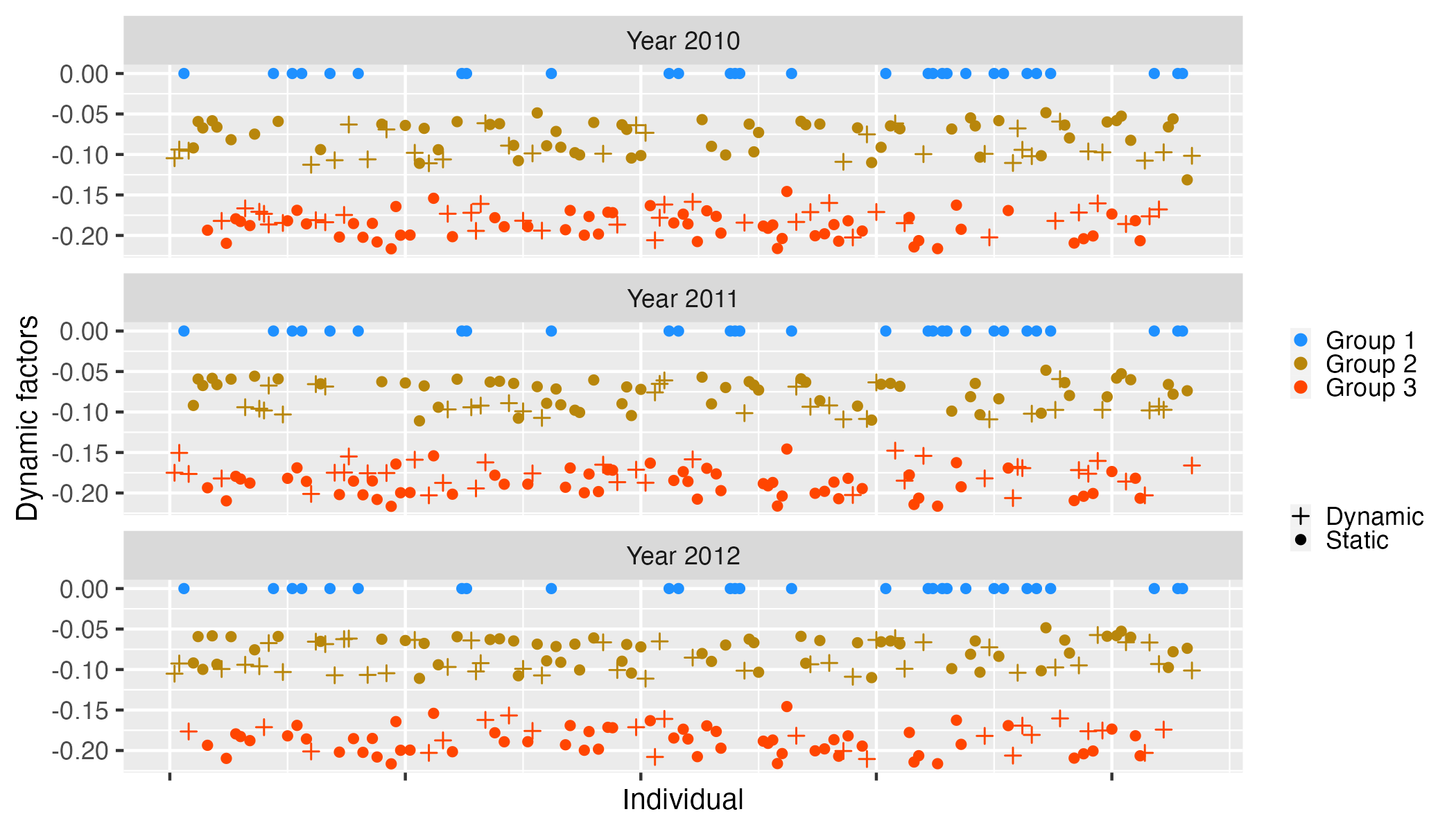
Figure 2: Recovered individual dynamic latent factor with group membership as well as membership patterns from 2010 to 2012. “Dynamic” indicates that the membership changes over time and “Static” indicates that the membership remains invariant over time.

Unlike gHIMA, which directly conducts subgroup analysis on the mediation effects, our approach involves clustering individuals in the latent space obtained from the low-rank decomposition of the coefficient matrix. As mentioned in Section 5.1, gHIMA only identifies the 3-group structure in 2 out of 100 replications. Based on this, we may infer that the subgroup structure might not be evident at the coefficient level but becomes clearer in the recovered latent space.

5.3 Individualized dynamic mediation effects

Finally, we analyze the detected significant mediators and evaluate the individualized dynamic mediation effects obtained by IDMA. Specifically, we detect 32 CpG sites with significant mediation effects. Excluding those CpG sites lying in intergenic regions (IGR), we identify 15 genes corresponding to these CpG sites (see Section LABEL:subsec:geneinfo of the Supplementary Materials for detailed information on all the detected CpG sites). We also compare the genes selected by IDMA with those selected by HIMA and gHIMA. Among these 15 genes, 5 genes (“KIAA1324L”, “PIK3C2G”, “CYP2W1”, “OR12D3”, and “HDAC”) are detected by all three methods and 5 genes (“ASCC3”, “SEC24B”, “DCX”, “PLB1”, and “WBP2NL”) are detected by both IDMA and HIMA. Additionally, 5 genes are detected exclusively by our IDMA, including “NXPH2”, “HLA-C”, ”RAP2C”, “FGD1”, and “UBE2W.”

Figure 3 illustrates the individualized dynamic mediation effects of 3 CpG sites corresponding to “NXPH2”, “HLA-C”, and “FGD1.” Results for genes ”RAP2C” and “UBE2W” are explained in Section LABEL:subsec:geneinfo of the Supplementary Materials. It is worth noting that different groups of individuals may exhibit distinct dynamic mediation patterns even for the same CpG site. Therefore, we group individuals based on the different dynamic patterns of their latent factors, as previously illustrated in Fig. 2, which results in 7 different trends.

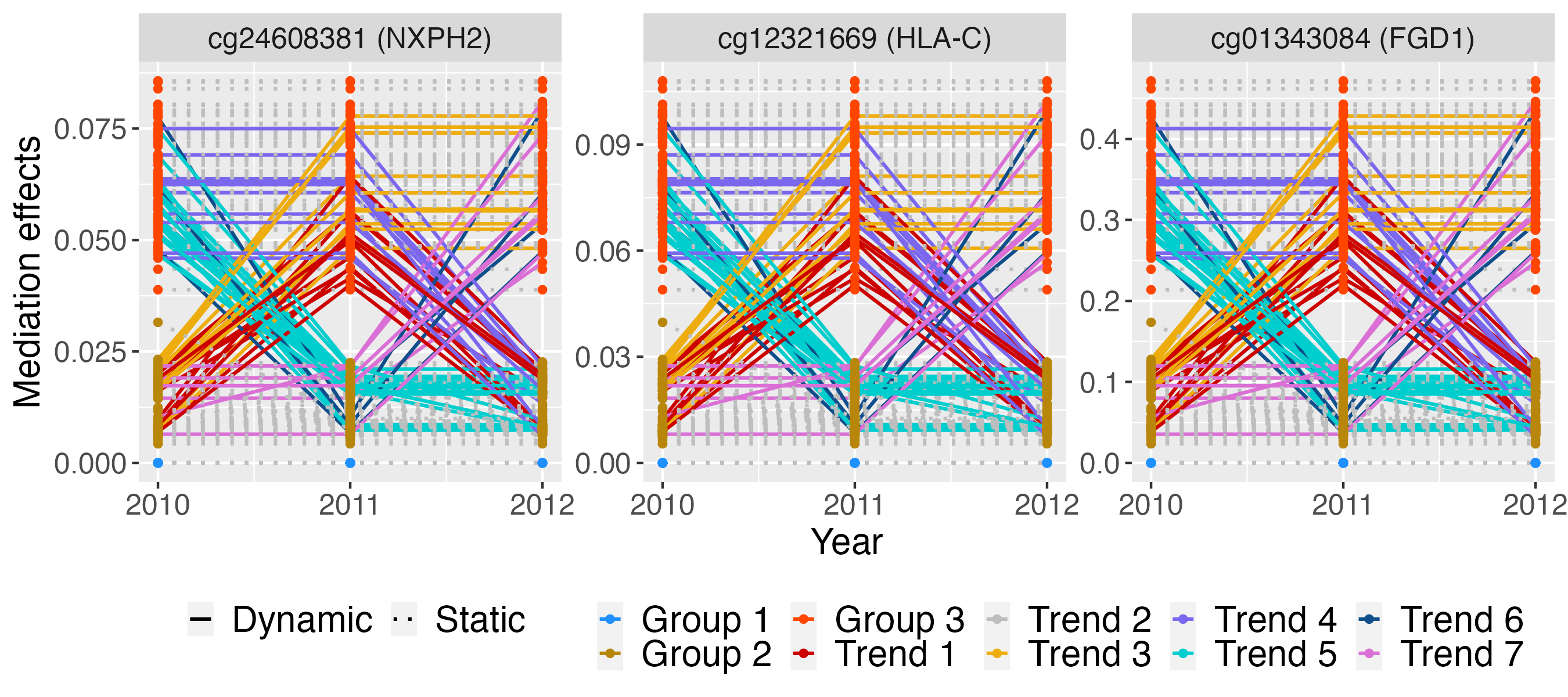
Figure 3: Individualized dynamic mediation effects of 3 CpG sites detected by IDMA only. Groups 1-3 align with subgroup memberships obtained in Section 5.2. “Dynamic” and “Static” denote whether an individual’s subgroup membership changes over time, consistent with Figure 2. Trends 1-7 represent different dynamic trends from 2010 to 2012.

Emerging studies have revealed a strong correlation between these genes and AD as well as depression. For instance, a recent study (Zhang et al., 2023) identified “NXPH2” as one of the top 10 most significant differentially methylated regions associated with CSF A$\beta_{42}$ in cognitively normal (CN) and AD subjects. Additionally, “NXPH2” has been identified as an informative gene for depressive disorders (Wang et al., 2023). Furthermore, research by Zipeto et al. (2018), Pandey et al. (2021), and a recent study (Gao et al., 2024) suggest that “HLA-C” variants are risk factors for AD and other neurodegenerative disorders. Further, a recent study in (Vică et al., 2022) also highlighted potential associations between HLA alleles and anxiety disorders. Regarding the gene “FGD1”, comparative transcriptome analysis of the hippocampus from sleep-deprived and AD mice (Wei, 2020) suggests that “FGD1” may play a crucial role in the development of human Alzheimer’s disease.

In general, our proposed IDMA shows advantages in prediction in both the mediator and the outcome model, while employing a more parsimonious model. Our method identifies relevant genes that have recently been found to be highly correlated with AD and also sheds light on potential genes related to AD. Additionally, our method identifies temporal mediation effect. Further details about the relationships between AD and the remaining 10 common genes detected by more than one method are provided in Section LABEL:subsec:geneinfo of the Supplementary Materials.

6 Discussion

We conclude the paper with three remarks. Firstly, our disentanglement of the coefficient matrices into individualized dynamic factors and mediator-specific loadings facilitates mediator selection and the information borrowing of adjacent temporal observations simultaneously. One can further explore replacing the structural assumption outlined in Section 2 with alternative structures on the mediators (e.g., homogeneity pursuit, (Ke et al., 2015), or the additive sparse and dense structure (Chernozhukov et al., 2017)), or on individuals separately, depending on prior knowledge.

Secondly, the number of measurements per individual considered in this paper is relatively small. For more intensive longitudinal studies, a potential approach could involve utilizing smoothing splines to exploit temporal information more effectively.

Thirdly, in this paper, we achieve disentanglement through matrix decomposition. However, a potential extension lies in employing encoder-decoder architecture from the deep learning literature. This extension could capture more complicated mediation mechanisms and offer an alternative direction to model the dynamics of the system.

References

- Avelar-Pereira et al. (2023) Avelar-Pereira, B., Belloy, M. E., O’Hara, R., Hosseini, S. H., and Alzheimer’s Disease Neuroimaging Initiative (2023). Decoding the heterogeneity of Alzheimer’s disease diagnosis and progression using multilayer networks. Molecular Psychiatry 28, 2423–2432.
- Bhootra et al. (2023) Bhootra, S., Jill, N., Shanmugam, G., Rakshit, S., and Sarkar, K. (2023). DNA methylation and cancer: Transcriptional regulation, prognostic, and therapeutic perspective. Medical Oncology 40, 71.
- Breiman (2001) Breiman, L. (2001). Random forests. Machine Learning 45, 5–32.
- Burer and Monteiro (2005) Burer, S. and Monteiro, R. D. (2005). Local minima and convergence in low-rank semidefinite programming. Mathematical Programming 103, 427–444.
- Cai et al. (2022) Cai, X., Coffman, D. L., Piper, M. E., and Li, R. (2022). Estimation and inference for the mediation effect in a time-varying mediation model. BMC Medical Research Methodology 22, 113.
- Candes and Plan (2010) Candes, E. J. and Plan, Y. (2010). Matrix completion with noise. Proceedings of the IEEE 98, 925–936.
- Chen (2015) Chen, Y. (2015). Incoherence-optimal matrix completion. IEEE Transactions on Information Theory 61, 2909–2923.
- Chen et al. (2020) Chen, Y., Chi, Y., Fan, J., Ma, C., and Yan, Y. (2020). Noisy matrix completion: Understanding statistical guarantees for convex relaxation via nonconvex optimization. SIAM Journal on Optimization 30, 3098–3121.
- Chernozhukov et al. (2017) Chernozhukov, V., Hansen, C., and Liao, Y. (2017). A lava attack on the recovery of sums of dense and sparse signals. The Annals of Statistics 45, 39 – 76.
- Chernozhukov et al. (2018) Chernozhukov, V., Hansen, C., Liao, Y., and Zhu, Y. (2018). Inference for heterogeneous effects using low-rank estimation of factor slopes. arXiv preprint arXiv:1812.08089 .
- Choi et al. (2024) Choi, J., Kwon, H., and Liao, Y. (2024). Inference for low-rank completion without sample splitting with application to treatment effect estimation. Journal of Econometrics 240, 105682.
- Delgado-Morales and Esteller (2017) Delgado-Morales, R. and Esteller, M. (2017). Opening up the DNA methylome of dementia. Molecular Psychiatry 22, 485–496.
- Dong et al. (2017) Dong, A., Toledo, J. B., Honnorat, N., Doshi, J., Varol, E., Sotiras, A., Wolk, D., Trojanowski, J. Q., Davatzikos, C., and Alzheimer’s Disease Neuroimaging Initiative (2017). Heterogeneity of neuroanatomical patterns in prodromal Alzheimer’s disease: Links to cognition, progression and biomarkers. Brain 140, 735–747.
- Dyachenko and Allenby (2023) Dyachenko, T. L. and Allenby, G. M. (2023). Is your sample truly mediating? Bayesian analysis of heterogeneous mediation (BAHM). Journal of Consumer Research 50, 116–141.
- Fan et al. (2022) Fan, J., Guo, J., and Zheng, S. (2022). Estimating number of factors by adjusted eigenvalues thresholding. Journal of the American Statistical Association 117, 852–861.
- Feinberg et al. (2006) Feinberg, A. P., Ohlsson, R., and Henikoff, S. (2006). The epigenetic progenitor origin of human cancer. Nature Reviews Genetics 7, 21–33.
- Fransquet et al. (2018) Fransquet, P. D., Lacaze, P., Saffery, R., McNeil, J., Woods, R., and Ryan, J. (2018). Blood DNA methylation as a potential biomarker of dementia: A systematic review. Alzheimer’s & Dementia 14, 81–103.
- Gao et al. (2024) Gao, Y., Su, B., Luo, Y., Tian, Y., Hong, S., Gao, S., Xie, J., and Zheng, X. (2024). HLA-C* 07: 01 and HLA-DQB1* 02: 01 protect against white matter hyperintensities and deterioration of cognitive function: A population-based cohort study. Brain, Behavior, and Immunity 115, 250–257.
- Guo et al. (2022) Guo, Z., Ćevid, D., and Bühlmann, P. (2022). Doubly debiased lasso: High-dimensional inference under hidden confounding. The Annals of statistics 50, 1320.
- Imai et al. (2010) Imai, K., Keele, L., and Yamamoto, T. (2010). Identification, inference and sensitivity analysis for causal mediation effects. Statistical Science 25, 51–71.
- Imai and Yamamoto (2013) Imai, K. and Yamamoto, T. (2013). Identification and sensitivity analysis for multiple causal mechanisms: Revisiting evidence from framing experiments. Political Analysis 21, 141–171.
- Jellinger (2022) Jellinger, K. A. (2022). Recent update on the heterogeneity of the Alzheimer’s disease spectrum. Journal of Neural Transmission 129, 1–24.
- Ke et al. (2015) Ke, Z. T., Fan, J., and Wu, Y. (2015). Homogeneity pursuit. Journal of the American Statistical Association 110, 175–194.
- Liu et al. (2018) Liu, X., Chen, X., Zeng, K., Xu, M., He, B., Pan, Y., Sun, H., Pan, B., Xu, X., Xu, T., et al. (2018). DNA-methylation-mediated silencing of miR-486-5p promotes colorectal cancer proliferation and migration through activation of PLAGL2/IGF2/-catenin signal pathways. Cell Death & Disease 9, 1037.
- Ma et al. (2011) Ma, S., Goldfarb, D., and Chen, L. (2011). Fixed point and Bregman iterative methods for matrix rank minimization. Mathematical Programming 128, 321–353.
- Negahban et al. (2012) Negahban, S. N., Ravikumar, P., Wainwright, M. J., and Yu, B. (2012). A unified framework for high-dimensional analysis of -estimators with decomposable regularizers. Statistical Science 27, 538–557.
- Pandey et al. (2021) Pandey, J. P., Nietert, P. J., Kothera, R. T., Barnes, L. L., and Bennett, D. A. (2021). Interactive effects of HLA and GM alleles on the development of Alzheimer disease. Neurology: Genetics 7, e565.
- Park et al. (2022) Park, S., Lee, E. R., and Zhao, H. (2022). Low-rank regression models for multiple binary responses and their applications to cancer cell-line encyclopedia data. Journal of the American Statistical Association pages 1–15.
- Perera et al. (2022) Perera, C., Zhang, H., Zheng, Y., Hou, L., Qu, A., Zheng, C., Xie, K., and Liu, L. (2022). HIMA2: High-dimensional mediation analysis and its application in epigenome-wide DNA methylation data. BMC Bioinformatics 23, 1–14.
- Pritchard (2001) Pritchard, J. K. (2001). Are rare variants responsible for susceptibility to complex diseases? The American Journal of Human Genetics 69, 124–137.
- Rusiecki et al. (2013) Rusiecki, J. A., Byrne, C., Galdzicki, Z., Srikantan, V., Chen, L., Poulin, M., Yan, L., and Baccarelli, A. (2013). PTSD and DNA methylation in select immune function gene promoter regions: A repeated measures case-control study of US military service members. Frontiers in Psychiatry 4, 56.
- Tang et al. (2021) Tang, X., Xue, F., and Qu, A. (2021). Individualized multidirectional variable selection. Journal of the American Statistical Association 116, 1280–1296.
- Tian et al. (2017) Tian, Y., Morris, T. J., Webster, A. P., Yang, Z., Beck, S., Feber, A., and Teschendorff, A. E. (2017). ChAMP: Updated methylation analysis pipeline for Illumina BeadChips. Bioinformatics 33, 3982–3984.
- Tibshirani (2014) Tibshirani, R. J. (2014). Adaptive piecewise polynomial estimation via trend filtering. The Annals of Statistics 42, 285 – 323.
- Tibshirani and Taylor (2011) Tibshirani, R. J. and Taylor, J. (2011). The solution path of the generalized lasso. The Annals of Statistics 39, 1335 – 1371.
- VanderWeele and Tchetgen Tchetgen (2017) VanderWeele, T. J. and Tchetgen Tchetgen, E. J. (2017). Mediation analysis with time varying exposures and mediators. Journal of the Royal Statistical Society Series B: Statistical Methodology 79, 917–938.
- Vică et al. (2022) Vică, M. L., Delcea, C., Dumitrel, G. A., Vușcan, M. E., Matei, H. V., Teodoru, C. A., and Siserman, C. V. (2022). The influence of HLA alleles on the affective distress profile. International Journal of Environmental Research and Public Health 19, 12608.
- Wang et al. (2021) Wang, W., Xu, J., Schwartz, J., Baccarelli, A., and Liu, Z. (2021). Causal mediation analysis with latent subgroups. Statistics in Medicine 40, 5628–5641.
- Wang et al. (2023) Wang, Y., Sun, Z., He, Q., Li, J., Ni, M., and Yang, M. (2023). Self-supervised graph representation learning integrates multiple molecular networks and decodes gene-disease relationships. Patterns 4,.
- Wei (2020) Wei, Y. (2020). Comparative transcriptome analysis of the hippocampus from sleep-deprived and Alzheimer’s disease mice. Genetics and Molecular Biology 43, e20190052.
- Xue et al. (2022) Xue, F., Tang, X., Kim, G., Koenen, K. C., Martin, C. L., Galea, S., Wildman, D., Uddin, M., and Qu, A. (2022). Heterogeneous mediation analysis on epigenomic ptsd and traumatic stress in a predominantly african american cohort. Journal of the American Statistical Association 117, 1669–1683.
- Yuan and Qu (2023) Yuan, Y. and Qu, A. (2023). De-confounding causal inference using latent multiple-mediator pathways. Journal of the American Statistical Association pages 1–28. (just-accepted).
- Zhang et al. (2016) Zhang, H., Zheng, Y., Zhang, Z., Gao, T., Joyce, B., Yoon, G., Zhang, W., Schwartz, J., Just, A., Colicino, E., et al. (2016). Estimating and testing high-dimensional mediation effects in epigenetic studies. Bioinformatics 32, 3150–3154.
- Zhang et al. (2023) Zhang, W., Young, J. I., Gomez, L., Schmidt, M. A., Lukacsovich, D., Varma, A., Chen, X. S., Martin, E. R., and Wang, L. (2023). Distinct csf biomarker-associated DNA methylation in Alzheimer’s disease and cognitively normal subjects. Alzheimer’s Research & Therapy 15, 78.
- Zhao et al. (2022) Zhao, B., Fan, Q., Liu, J., Yin, A., Wang, P., and Zhang, W. (2022). Identification of key modules and genes associated with major depressive disorder in adolescents. Genes 13, 464.
- Zheng et al. (2021) Zheng, Z., Lv, J., and Lin, W. (2021). Nonsparse learning with latent variables. Operations Research 69, 346–359.
- Zipeto et al. (2018) Zipeto, D., Serena, M., Mutascio, S., Parolini, F., Diani, E., Guizzardi, E., Rizzardo, S., Malena, M., Romanelli, M. G., Tamburin, S., et al. (2018). Hiv-1-associated neurocognitive disorders: is HLA-C binding stability to 2-microglobulin a missing piece of the pathogenetic puzzle? Frontiers in Neurology 9, 409207.
- Zou and Li (2008) Zou, H. and Li, R. (2008). One-step sparse estimates in nonconcave penalized likelihood models. The Annals of Statistics 36, 1509.