Optimizing Layout of Recursive Datatypes with Marmoset

Abstract

While programmers know that the low-level memory representation of data structures can have significant effects on performance, compiler support to optimize the layout of those structures is an under-explored field. Prior work has optimized the layout of individual, non-recursive structures without considering how collections of those objects in linked or recursive data structures are laid out.

This work introduces Marmoset, a compiler that optimizes the layouts of algebraic datatypes, with a special focus on producing highly optimized, packed data layouts where recursive structures can be traversed with minimal pointer chasing. Marmoset performs an analysis of how a recursive ADT is used across functions to choose a global layout that promotes simple, strided access for that ADT in memory. It does so by building and solving a constraint system to minimize an abstract cost model, yielding a predicted efficient layout for the ADT. Marmoset then builds on top of Gibbon, a prior compiler for packed, mostly-serial representations, to synthesize optimized ADTs. We show experimentally that Marmoset is able to choose optimal layouts across a series of microbenchmarks and case studies, outperforming both Gibbon’s baseline approach, as well as MLton, a Standard ML compiler that uses traditional pointer-heavy representations.

1 Introduction

Recursive data structures are readily available in most programming languages. Linked lists, search trees, tries and others provide efficient and flexible solutions to a wide class of problems—both in low-level languages with direct memory access (C, C++, Rust, Zig) as well as high-level ones (Java, C , Python). Additionally, in the purely functional (or persistent [20]) setting, recursive, tree-like data structures largely replace array-based ones. Implementation details of recursive data structures are not necessarily known to application programmers, who can only hope that the library authors and the compiler achieve good performance. Sadly, recursive data structures are a hard optimization target.

High-level languages represent recursive structures with pointers to small objects allocated sparsely on the heap. An algorithm traversing such a boxed representation spends much time in pointer chasing, which is a painful operation for modern hardware architectures. Optimizing compilers for these languages and architectures have many strengths but optimizing memory representation of user-defined data structures is not among them. One alternative is resorting to manual memory management to achieve maximum performance, but it has the obvious drawback of leaving convenience and safety behind.

A radically different approach is representing recursive datatypes as dense structures (basically, arrays) with the help of a library or compiler. The Gibbon compiler tries to improve the performance of recursive data structures by embracing dense representations by default [24]. This choice has practical benefits for programmers: they no longer need to take control of low-level data representation and allocation to serialize linked structures; and rather than employing error-prone index arithmetic to access data, they let Gibbon automatically translate idiomatic data structure accesses into operations on the dense representation.

Dense representations are not a panacea, though. They can suffer a complementary problem due to their inflexibility. A particular serialization decision for a data structure made by the compiler can misalign with the behavior of functions accessing that data. Consider a tree laid out in left-to-right pre-order with a program that accesses that tree right-to-left. Rather than scanning straightforwardly through the structure, the program would have to jump back and forth through the buffer to access the necessary data.

One way to counter the inflexibility of dense representations is to introduce some pointers. For instance, Gibbon inserts shortcut pointers to allow random access to recursive structures [23]. But this defeats the purpose of a dense representation: not only are accesses no longer nicely strided through memory, but the pointers and pointer chasing of boxed data are back. Indeed, when Gibbon is presented with a program whose access patterns do not match the chosen data layout, the generated code can be significantly slower than a program with favorable access patterns.

Are we stuck with pointer chasing when processing recursive data structures? We present Marmoset as a counter example. Marmoset is our program analysis and transformation approach that spots misalignments of algorithms and data layouts and fixes them where possible. Thus, our slogan is:

Algorithms + Data Layouts = Efficient Programs

Marmoset analyzes the data access patterns of a program and synthesizes a data layout that corresponds to that behavior. It then rewrites the datatype and code to produce more efficient code that operates on a dense data representation in a way that matches access patterns. This co-optimization of datatype and code results in improved locality and, in the context of Gibbon, avoidance of shortcut pointers as much as possible.

We implement Marmoset as an extension to Gibbon—a compiler based on dense representations of datatypes. That way, Marmoset can be either a transparent compiler optimization, or semi-automated tool for exploring different layouts during the programmer’s optimization work. Our approach has general applicability because of the minimal and common nature of the core language: the core language of Marmoset (Figure 4) is a simple first-order, monomorphic, strict, purely functional language. Thanks to the succinct core language, we manage to isolate Marmoset from Gibbon-specific, complicated (backend) mechanics of converting a program to operate on dense rather than boxed data.

Overall, in this paper:

• We provide a static analysis capturing the temporal access patterns of a function towards a datatype it processes. As a result of the analysis, we generate a field access graph that summarizes these patterns.

• We define a cost model that, together with the field access graph, enables formulating the field-ordering optimization problem as an integer linear program. We apply a linear solver to the problem and obtain optimal positions of fields in the datatype definition relative to the cost model.

• We extend the Gibbon compiler to synthesize new datatypes based on the solution to the optimization problem, and transform the program to use these new, optimized types, adjusting the code where necessary.

• Using a series of benchmarks, we show that our implementation, Marmoset, can provide speedups of 1.14 to 54 times over the best prior work on dense representations, Gibbon. Marmoset outperforms MLton on these same benchmarks by a factor of 1.6 to 38.

2 Dense Representation: The Good, The Bad, and The Pointers

This section gives a refresher on dense representations of algebraic datatypes (Section 2.1) and, using an example, illustrates the performance challenges of picking a layout for a datatype’s dense representation (Section 2.2).

2.1 Overview

Algebraic datatypes (ADTs) are a powerful language-based technology. ADTs can express many complex data structures while, nevertheless, providing a pleasantly high level of abstraction for application programmers. The high-level specification of ADTs leaves space to experiment with low-level implementation strategies. Hence, we use ADTs and a purely functional setting for our exploration of performance implications of data layout.

In a conventional implementation of algebraic datatypes, accessing a value of a given ADT requires dereferencing a pointer to a heap object, then reading the header word, to get to the payload. Accessing the desired data may require multiple further pointer dereferences, as objects may contain pointers to other objects, requiring the unraveling of multiple layers of nesting. The whole process is often described as pointer chasing, a fitting name, especially when the work per payload element is low.

In a dense representation of ADTs, as implemented in Gibbon, the data constructor stores one byte for the constructor’s tag, followed immediately by its fields, in the hope of avoiding pointer chasing. Wherever possible, the tag value occurs inline in a bytestream that hosts multiple values. As a result, values tend to reside compactly in the heap using contiguous blocks of memory. This representation avoids or reduces pointer chasing and admits efficient linear traversals favored by modern hardware via prefetching and caching.

2.2 Running Example

The efficiency of traversals on dense representations of data structures largely depends on how well access patterns and layout match each other. Consider a datatype (already monomorphized) describing a sequence of posts in a blog:

⬇

data BlogList = Nil $\mid$ Blog Content HashTags BlogList

A non-empty blog value stores a content field (a string representing the body of the blog post), a list of hash tags summarizing keywords of the blog post, and a pointer to the rest of the list.. The datatype has one point of recursion and several variable-length fields in the definition. To extend on this, Section 5.3.4 contains an example of tree-shaped data (two points of recursion, in particular) with a fixed-length field. The most general case of multiple points of recursion and variable-length fields is also handled by Marmoset.

The most favorable traversal for the Blog datatype is the same as the order in which the fields appear in the datatype definition. In this case, Gibbon can assign the dense and pointer-free layout as shown in Figure 2(a). Solid blue arrows connecting adjacent fields represent unconditional sequential accesses—i.e., reading a range of bytes in a buffer, and then reading the next consecutive range. Such a traversal will reap the benefits of locality.

⬇

emphKeyword :: String $\rightarrow$ BlogList $\rightarrow$ BlogList

emphKeyword keyword blogs = case blogs of

Nil $\rightarrow$ Nil

Blog content hashTags blogs' $\rightarrow$

case search keyword hashTags of

True $\rightarrow$ let content' = emphContent content keyword

blogs'' = emphKeyword keyword blogs'

in Blog content' hashTags blogs''

False $\rightarrow$ let blogs'' = emphKeyword keyword blogs'

in Blog content hashTags blogs''

Figure 1: Blog traversal motivating example

On the other hand, consider a traversal with less efficient access patterns (Figure 1). The algorithm scans blog entries for a given keyword in HashTags. If the hash tags of a particular blog entry contain the keyword, the algorithm puts an emphasis on every occurrence of the keyword in the content field. In terms of access patterns, if we found a match in the hash tags field, subsequent accesses to the fields happen in order, as depicted in Figure 2(b). Otherwise, the traversal skips over the content field, as depicted in Figure 2(c).

Here we use red lines to represent accesses that must skip over some data between the current position in the buffer and the target data. Data may be constructed recursively and will not necessarily have a statically-known size, so finding the end of a piece of unneeded data requires scanning through that data in order to reach the target data. This extra traversal (parsing data just to find the end of it) requires an arbitrarily large amount of work because the content field has a variable, dynamically-allocated size.

Extra traversals that perform useful no work, like skipping over the content field above, can degrade the asymptotic efficiency of programs. One way to avoid such traversals is to use pointers. For instance, when Gibbon detects that it has to skip over intervening data, it changes the definition of the constructor by inserting shortcut pointers, which provide an exact memory address to skip to in constant time. For our example program, Gibbon introduces one shortcut pointer for the HashTags field, and another one for the tail of the list.

The pointers provide direct accesses to the respective fields when needed and restore the constant-time asymptotic complexity for certain operations. This results in the access patterns shown in Figure 3(a) and 3(c). Red dashed lines represent pointer-based constant-time field accesses. Otherwise, the access patterns are similar to what we had before.

The pointer-based approach in our example has two weaknesses. First, this approach is susceptible to the usual problems with pointer chasing. Second, just like with the initial solution, we access fields in an order that does not match the layout: the hash tags field is always accessed first but lives next to the content field.

Marmoset, described in the following section, automates the process of finding the weaknesses of the pointer-based approach and improving the layout and code accordingly. For instance, performance in our example can be improved by swapping the ordering between the Content and HashTags fields. Given this reordering, the hash tags are available directly at the start of the value, which lines up with the algorithm better, as the algorithm always accesses this field first. Additionally, our program’s True case (the keyword gets a hit within the hash tags) is more efficient because after traversing the content to highlight the keyword it stops at the next blog entry ready for the algorithm to make the recursive call. This improved data layout results in the more-streamlined access patterns shown in Figures 3(b) and 3(d).

(a) Ideal access patterns

(b) True case extra traversals

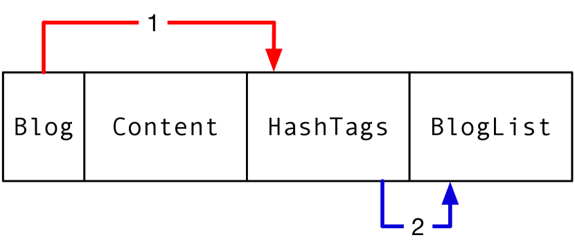
(c) False case extra traversals

Figure 2: Showing a dense pointer-free layout with ideal accesses on top. Numbers represent the access order. Out of order accesses (red), incur costly extra traversals over fields in the middle.

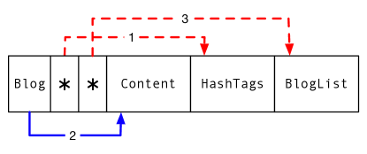
(a) True case unoptimized

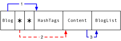
(b) True case optimized

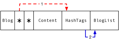
(c) False case unoptimized

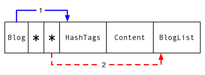
(d) False case optimized

Figure 3: Showing the unoptimized representation with pointers to allow random access and the optimized layout with favorable access patterns.

3 Design

Marmoset infers efficient layouts for dense representations of recursive datatypes. Marmoset’s key idea is that the best data layout should match the way a program accesses these data. Section 2 shows how this idea reduces to finding an ordering of fields in data constructors. The ordering must align with the order a function accesses those fields, in which case the optimization improves performance of the function.

To find a better layout for a datatype in the single-function case, Marmoset first analyzes possible executions of the function and their potential for field accesses. In particular, Marmoset takes into account (a) the various paths through a function, each of which may access fields in a different order, and (b) dependencies between operations in the function, as in the absence of dependencies, the function can be rewritten to access fields in the original order, and that order will work best. Marmoset thus constructs a control-flow graph (Section 3.2) and collects data-flow information (Section 3.3) to build a field access graph, a representation of the various possible orders in which a function might access fields (Section 3.4 and Section 3.5).

Once data accesses in a function are summarized in the field access graph, Marmoset proceeds with synthesizing a data layout. Marmoset incorporates knowledge about the benefits of sequential, strided access and the drawbacks of pointer chasing and backtracking to define an abstract cost model. The cost model allows to formulate an integer linear program whose optimal solution corresponds to a layout that minimizes the cost according to that model (Section 3.6).

The remainder of this section walks through this design in detail, and discusses how to extend the system to handle multiple functions that use a datatype (Section 3.7).

3.1 Marmoset’s Language

Marmoset operates on the language $\lambda_{M}$ given in Figure 4. $\lambda_{M}$ is a first-order, monomorphic, call-by-value functional language with algebraic datatypes and pattern matching. Programs consist of a series of datatype definitions, function definitions, and a main expression. $\lambda_{M}$’s expressions use A-normal form [12]. The notation $\overline{x}$ denotes a vector $[x_{1},\ldots,x_{n}]$ and $\overline{x_{\mathit{i}}}$ the item at position $\mathit{i}$. $\lambda_{M}$ is an intermediate representation (IR) used towards the front end in the Gibbon compiler. The monomorphizer and specializer lower a program written in a polymorphic, higher-order subset of Haskell to $\lambda_{M}$, and then location inference is used to convert it to the location calculus (LoCal) code next [23]. It is easier to update the layout of types in $\lambda_{M}$ compared to LoCal, as in $\lambda_{M}$ the layout is implicitly determined by the ordering of fields, whereas the later LoCal IR makes the layout explicit using locations and regions (essentially, buffers and pointer arithmetic).

$$\mathit{K}\in\;\textup{Data Constructors},\>\>\mathit{\tau}\in\;\textup{Type Constructors},\>\>x,y,f\in\;\textup{Variables}$$

Top-Level Programs $$\mathit{top} \;::= \overline{\mathit{dd}}\;;\overline{\mathit{fd}}\;;\mathit{e}$$

Field of a Data Constructor $$\mathit{fe} \;::= \mathit{\tau}$$

Datatype Declarations $$\mathit{dd} \;::= \texttt{data}\;\mathit{\tau}=\overline{\mathit{K}\;\overline{\mathit{fe}}\;}$$

Function Declarations $$\mathit{fd} \;::= f:\overline{\mathit{\tau}}\rightarrow\mathit{\tau};f\;\overline{x}=\mathit{e}$$

Values $$\mathit{v} \;::= x$$

Expressions $$\mathit{e} \;::= \mathit{v}$$

$$\;| \texttt{let}\;x:\mathit{\tau}=f\;\overline{\mathit{v}}\;\texttt{in}\;\mathit{e}$$

$$\;| \texttt{let}\;x:\mathit{\tau}=\mathit{K}\;\overline{\mathit{v}}\;\texttt{in}\;\mathit{e}$$

$$\;| \texttt{case}\;\mathit{v}\;\texttt{of}\;\overline{\mathit{pat}}$$

Pattern $$\mathit{pat} \;::= \mathit{K}\;\;(\overline{x:\mathit{\tau}})\;\rightarrow\;\mathit{e}$$

Figure 4: Simplified grammar for a first-order, monomorphic functional language that Marmoset operates on. The full implementation includes more primitive datatypes, and built in primitives (such as a copy primitive).

3.2 Control-Flow Analysis

Algorithm 1 Control-Flow Graph Psuedocode

1:Input

2:    exp: An expression in subset of $\lambda_{M}$

3:    weight: The likelyhood of exp executing (i.e., exp’s inbound edge)

4:Output

5:    A tuple of list of cfg nodes and the node id.

6:function ControlFlowGraph(exp, weight)

7:    let nodeId = genFreshId()

8:    switch $exp$ do

9:         case LetE (v, ty, rhs) bod

10:             let (nodes, succId) = ControlFlowGraph(bod, weight)

11:             let newNode = (nodeId, (LetRHS (v, ty, rhs), weight), [succId])

12:             return (nodes ++ newNode, nodeId)

13:         end case

14:         case CaseE scrt cases

15:             let (nodes, successors) = CfgCase(weight/length(cases), cases)

16:             let newNode = (nodeId, (scrt, weight), successors)

17:             return (nodes ++ [newNode], nodeId)

18:         end case

19:         case VarE v

20:             let newNode = (nodeId, (v, weight), [])

21:             return ([newNode], nodeId)

22:         end case

23:    end switch

24:end function

We construct a control-flow graph with sub-expressions, and let-bound RHS’s (right hand sides) of $\lambda_{M}$ as the nodes. Algorithm 1 shows the psuedocode for generating the control-flow graph. Because the syntax is flattened into A-normal form, there is no need to traverse within the RHS of a let expression. Edges between the nodes represent paths between expressions. The edges consist of weights (Line 11) that represent the likelihood of a particular path being taken. An edge between two nodes indicates the order of the evaluation of the program. A node corresponding to a let-binding (Line 9) contains the bound expression and has one outgoing edge to a node corresponding to the body expression. A case expression (Line 14) splits the control flow $n$-ways, where $n$ is the number of pattern matches. Outgoing edges of a node for a case expression have weights associated with them that correspond to the likelihood of taking a particular branch in the program. If available, dynamic profiling information can provide these weights. For the purposes of this paper, however, we find it is sufficient to use trivial placeholder weights: i.e. uniform weight over all branches. Control flow terminates on a variable reference $\lambda_{M}$ expression.

Figure 5(a) shows the control-flow graph for the running example from Figure 1. Each node corresponds to a sub-expression of the function emphKeyword. The first case expression splits the control flow into two branches, corresponding to whether the input list of blogs is empty or not. The branch corresponding to the empty input list is assigned a probability $\alpha$, and thus, the other branch is assigned a probability $1-\alpha$. The next node corresponds to the pattern match Blog content hashTags blogs'. Another two-way branch follows, corresponding to whether keyword occurs in the content of this blog or not. We assign the probabilities $\sigma$ and $1-\sigma$ to these branches respectively. Note that as a result, the corresponding edges in the CFG have weights $(1-\alpha)*\sigma$ and $(1-\alpha)*(1-\sigma)$, as the likelihood of reaching that condition is $(1-\alpha)$. Each of these branches terminate by creating a new blog entry with its content potentially updated. In the current model, $\alpha$ and $\sigma$ are 0.5: they are uniformly distributed.

One intuition for why realistic branch weights are not essential to Marmoset’s optimization is that accurate weights only matter if there is a trade off between control-flow paths that are best served by different layouts. The base cases (e.g. empty list) typically contribute no ordering constraints, and in our experience, traversals tend to have a preferred order per function, rather than tradeoffs intra-function, which would reward having accurate, profile-driven branch probabilities. Hence, for now, we use uniform weights even when looking at the intra-function optimization.

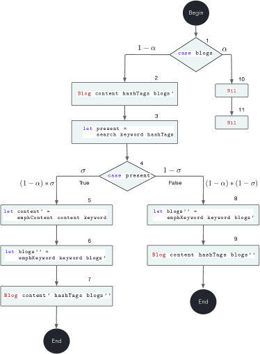
(a) CFG with probability of executing along each path.

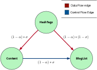
(b) Field-access graph $G$ generated from control-flow graph. Here we use field types to uniquely name them, since Haskell record syntax was not used in this example to give each field a name.

Figure 5: Control-flow and corresponding field access graphs generated for the running example

3.3 Data Flow Analysis

We implement a straightforward analysis (use-def chain, and def-use chain) for let expressions to capture dependencies between let expressions. We use this dependence information to form dataflow edges in the field access graph (Section 3.5) and to subsequently optimize the layout and code of the traversal for performance. For independent let expressions in the function we are optimizing, we can transform the function body to have these let expressions in a different order. (Independent implies that there are no data dependencies between such let expressions. Changing the order of independent let expressions will not affect the correctness of code, modulo exceptions.) However, we do such a transformation only when we deem it to be more cost efficient. In order to determine when re-ordering let expressions is more cost efficient, we classify fields based on specific attributes next.

3.4 Field Attributes For Code Motion

When trying to find the best layout, we may treat the code as immutable, but allowing ourselves to move the code around (i.e. change the order of accesses to the fields) unlocks more possibilities for the resulting layout. Not all code motions are valid due to existing data dependencies in the traversal. For instance, in a sequence of two let binders, the second one may reference the binding introduced in the first one: in this case, the two binders cannot be reordered.

To decide which code motions are allowed, we classify each field with one or more of the attributes: recursive, scalar, self-recursive, or inlineable. Some of these attributes are derived from the ADT definition and some from the code using the ADT. A scalar field refers to a datatype only made up of either other primitive types, such as Int. A recursive field refers to a datatype defined recursively. A self-recursive field is a recursive field that directly refers back to the datatype being defined (such as a List directly referencing itself). Finally, we call a field inlineable if the function being optimized makes a recursive call into this field (i.e. taking the field value as an argument). Hence, an inlineable field is necessarily a recursive field. As we show in the example below, the inlineable attribute is especially important when choosing whether or not to do code motion.

A single field can have multiple attributes. For instance, a function (traverse) doing a pre-order traversal on a Tree datatype makes recursive calls on both the left and right children. The left and right children are recursive and self-recursive. Therefore, when looking at the scope of traverse, the left and right children have the attributes recursive, self-recursive and inlineable.

⬇

foo :: List $\rightarrow$ List

foo lst = case lst of

Nil $\rightarrow$ Nil

Cons x rst $\rightarrow$

let x' = x ^ 100

rst' = foo rst

in Cons x' rst'

(a) Function foo with List.

⬇

foo' :: List' $\rightarrow$ List'

foo' lst = case lst of

Nil' $\rightarrow$ Nil'

Cons' rst x $\rightarrow$

let rst' = foo' rst

x' = x ^ 100

in Cons' rst' x'

(b) Function foo' with List'.

Figure 6: Two different traversals on a list.

Example. Consider the example of a list traversal shown in Figure 6(a). Here the function foo does some work on the Int field (it raises the Int to the power of 100) and then recurs on the tail of the list. Note that Marmoset is compiling with dense representations, i.e., List type is going to be packed in memory with a representation that stores the Cons tag (one byte) followed by the Int (8 bytes) followed by the next Cons tag and so on. Hence, the Cons tag and the Int field are interleaved together in memory. The function foo becomes a stream processor that consumes one stream in memory and produces a dense output buffer of the same type.

On the other hand, the other way to lay out the list is to change its representation to the following.

⬇

data List' = Nil' $\mid$ Cons' List' Int

In memory, the list has all Cons' tags next to each other (a unary encoding of array length!) and the Int elements all next to each other. In such a scenario, the performance of our traversal foo on the List' can improve traversal performance due to locality when accessing elements stored side-by-side. However, this only works if we can subsequently change the function that traverses the list to do recursion on the tail of the list first and then call the exponentiation function on the Int field after the recursive call. If there are no data dependencies between the recursive call and the exponentiation function, then this is straightforward. We show foo' with the required code motion transformation to function foo accompanied with the change in the data representation from List to List' as shown in Figure 6(b).

To optimize the layout, the tail of the list is assigned the attribute of inlineable. This attribute is used by the solver to determine a least-cost ordering to the List datatype in the scope of function foo. Whenever such code motion is possible, Marmoset will place the inlineable field first and use code-motion to change the body of the function to perform recursion first if data flow dependencies allow such a transformation.

Structure of arrays. The transformation of List/foo to List'/foo' is similar to changing the representation of the List datatype to a structure of arrays, which causes the same types of values to be next to each other in memory. In particular, we switch from alternating constructor tags and integer values in memory to an array of constructor tags followed by an array of integers.

Note that the traversals foo and foo' have access patterns that are completely aligned with the data layout of List and List' respectively. The resulting speedup is solely a consequence of the structure of arrays effect. This is an added benefit to the runtime in addition to ensuring that the access patterns of a traversal are aligned with the data layout of the datatype it traverses.

3.5 Field Access Pattern Analysis

Algorithm 2 Recursive function for generating the field access graph

1:Input

2:    cur: current CFG node from which to start processing

3:    dcon: data constructor for which we are searching the best layout

4:    edges: field-access graph built so far

5:    lastAccessedVar: last accessed variable name, initially None

6:    dfgMap: set of data-flow edges between variables

7:Output

8:    Field access graph represented as a list of edges

9:function FieldAccessGraph(cur, dcon, edges, lastAccessedVar, dfgMap)

10:    let ((expr, weight), successors) = cur

11:    let mutable lastAccessedVarMut = lastAccessedVar

12:    let mutable edges'= edges

13:    for var : OrderedFreeVariables(expr) do

14:         if !BoundInPatternMatchOnDcon(var, dcon) then

15:             continue

16:         end if

17:         if lastAccessedVarMut != None then

18:             mutate edges'= addEdge(edges', ((lastAccessedVar, var), weight), CfgTag)

19:             if lookup((lastAccessedVar, var), dfgMap) then

20:                 mutate edges'= addEdge(edges', ((lastAccessedVar, var), weight), DfgTag)

21:             end if

22:         end if

23:         mutate lastAccessedVarMut = var

24:    end for

25:    for succ : successors do

26:         let edges''= FieldAccessGraph(succ, dcon, edges', lastAccessedVarMut, dfgMap)

27:         mutate edges'= merge(edges', edges'')

28:    end for

29:    return edges'

30:end function

After constructing the CFG and DFG for a function definition, we utilize them to inspect the type of each of the function’s input parameters—one data constructor at a time—and construct a field-access graph for it. Algorithm 2 shows the psuedocode for generating the field-access graph. This graph represents the temporal ordering of accesses among its fields.

The fields of the data constructor form the nodes of this graph. A directed edge from field $f_{i}$ to field $f_{j}$ is added if $f_{i}$ is accessed immediately before $f_{j}$. Lines 13 to  24 in Algorithm 2 show how we keep track of the last accessed field and form an edge if possible. A directed edge can be of two different types. In addition, each edge has a associated weight which indicates the likelihood of accessing $f_{i}$ before $f_{j}$, which is computed using the CFG. An edge can either be a data-flow edge or a control-flow edge (Lines 18 and  20). In Figure 5(b), the red edge is a data flow edge and the blue edge is a control flow edge.

Data-Flow Edge indicates an access resulting from a data flow dependence between the fields $f_{i}$ and $f_{j}$. In our source language, a data flow edge is induced by a case expression. A data flow edge implies that the code that represents the access is rigid in structure and changing it can make our transformation invalid.

Control-Flow Edge indicates an access that is not data-flow dependent. It is caused by the control flow of the program. Such an edge does not induce strict constraints on the code that induces the edge. The code is malleable in case of such accesses. This gives way to an optimization search space via code motion of let expressions. The optimization search space involves transformation of the source code, i.e, changing the access patterns at the source code level.

The field-access graph $G$ is a directed graph, which consists of edges of the two types between fields of a datatype and can have cycles. The directed nature of the edges enforces a temporal relation between the corresponding fields. More concretely, assume that an edge $e$ that connects two vertices representing fields $\mathit{fe}_{a}$ (source of $e$) and $\mathit{fe}_{b}$ (target of $e$). We interpret $e$ as an evidence that field $\mathit{fe}_{a}$ is accessed before field $\mathit{fe}_{b}$. The weight $w$ for the edge $e$ is the probability that this access will happen based on statically analyzing a function.

In our analysis, for a unique path through the traversal, we only account for the first access to any two fields. If two fields are accessed in a different order later on, the assumption is that the start address of the fields is likely to be in cache and hence it does not incur an expensive fetch call to memory. In fact, we tested our hypothesis by artificially making an example where say field $f_{a}$ is accessed first, field $f_{b}$ is accessed after $f_{a}$ after which we constructed multiple artificial access edges from $f_{b}$ to $f_{a}$, which might seem to suggest placing $f_{b}$ before $f_{a}$. However, once the cache got warmed up and the start addresses of $f_{a}$ and $f_{b}$ are already in cache, the layout did not matter as much. This suggests that prioritizing for the first access edge between two unique fields along a unique path is sufficient for our analysis.

Two fields can be accessed in a different order along different paths through a traversal. This results in two edges between the fields. (The edges are in reversed order.) We allow at most two edges between any two vertices with the constraint that they have to be in the opposite direction and come from different paths in the traversal. If two fields are accessed in the same order along different paths in the traversal, we simply add the probabilities and merge the edges since they are in the same direction.

In order to construct $G$, we topologically sort the control-flow graph of a function and traverse it in the depth-first fashion via recursion on the successors of the current cfg node (Lines 25 to 28). As shown in line 14, we check if a variable is an alias to a field in the data constructor for which we are constructing the field-access graph $G$. As we process each node (i.e. a primitive expression such as a single function call), we update the graph for any direct or indirect references to input fields that we can detect. We ignore new variable bindings that refer to newly allocated rather than input data—they are not tracked in the access graph. We traverse the control-flow graph once, but we maintain the last-accessed information at each CFG node, so when we process a field access at an expression, we consult what was previously-accessed at the unique precedecessor of the current CFG node. Figure 5(b) shows the generated access graph from the control-flow graph in Figure 5(a). It also shows the probability along each edge obtained from the control-flow graph.

As we are traversing the nodes of the control-flow graph and generating directed edges in $G$, we use the likelihood of accessing that cfg node as the weight parameter (Line 10).

3.6 Finding a Layout

We use the field-access graph $G$ to encode the problem of finding a better layout as an Integer Linear Program (ILP). Solving the problem yields a cost-optimal field order for the given pair of a data constructor and a function.

3.6.1 ILP Constraints

In our encoding, each field in the data constructor is represented by a variable, $f_{0},f_{1},\dots$ As a part of the result, each variable will be assigned a unique integer in the interval $[0,n-1]$, where $n$ is the number of fields. Intuitively, each variable represents an index in the sequence of fields.

The ILP uses several forms of constraints, including two forms of hard constraints:

$$\forall_{0\leq i<n}\qquad 0\leqslant f_{i}<n$$ (1)

$$\forall_{0\leq i<j<n}\qquad f_{i}\neq f_{j}$$ (2)

The constraints of form 1 ensure that each field is mapped to a valid index, while the constraints of form 2 ensure that each field has a unique index. Constraints of either form must hold because each field must be in a valid location.

Hard constraints define valid field orderings but not all such reorderings improve efficiency, Marmoset’s main goal. To fulfil the goal, beside the hard constraints we introduce soft ones. Soft constraints come from the field access analysis. For example, assume that based on the access pattern of a function, we would prefer that field $a$ goes before field $b$. We turn such a wish into a constraint. If the constraint cannot be satisfied, it will not break the correctness. In other words, such constraints can be broken, and that is why we call them soft.

3.6.2 Cost Model

Marmoset encodes these soft constraints in the form of an abstract cost model that assigns a cost to a given layout (assignment of fields to positions) based on how efficient it is expected to be given the field-access graph.

To understand the intuition behind the cost model, note that the existence of an edge from field $f_{i}$ to field $f_{j}$ in the field-access graph means that there exists at least one path in the control-flow graph where $f_{i}$ is accessed and $f_{j}$ is the next field of the data constructor that is accessed. In other words, the existence of such an edge implies a preference for that control-flow path for field $f_{i}$ to be immediately before field $f_{j}$ in the layout so that the program can continue a linear scan through the packed buffer. Failing that, it would be preferable for $f_{j}$ to be “ahead” of $f_{i}$ in the layout so the program does not have to backtrack in the buffer. We can thus consider the costs of the different layout possibilities of $f_{i}$ and $f_{j}$:

$C_{\mathit{succ}}$

($f_{j}$ immediately after $f_{i}$): This is the best case scenario: the program traverses $f_{i}$ and then uses $f_{j}$.

$C_{\mathit{after}}$

($f_{j}$ after $f_{i}$ in the buffer): If $f_{j}$ is after $f_{i}$, but not immediately after, then the code can proceed without backtracking through the buffer, but the intervening data means that either a shortcut pointer or a extra traversal must be used to reach $f_{j}$, adding overhead.

$C_{\mathit{pred}}$

($f_{j}$ immediately before $f_{i}$): Here, $f_{j}$ is earlier than $f_{i}$ in the buffer. Thus, the program will have already skipped past $f_{j}$, and some backtracking will be necessary to reach it. This incurs two sources of overhead: skipping past $f_{j}$ in the first place, and then backtracking to reach it again.

$C_{\mathit{before}}$

($f_{j}$ before $f_{i}$ in the buffer): If, instead, $f_{j}$ is farther back in the buffer than $f_{i}$, then the cost of skipping back and forth is greater: in addition to the costs of pointer dereferencing, because the fields are far apart in the buffer, it is less likely $f_{j}$ will have remained in cache (due to poorer spatial locality).

We note a few things. First, the exact values of each of these costs are hard to predict. The exact penalty a program would pay for jumping ahead or backtracking depends on a variety of factors such as cache sizes, number of registers, cache line sizes, etc.

However, we use our best intuition to statically predict these costs based on the previously generated access graph. Note the existence of two types of edges in our access graph. An edge can either be a data-flow edge or a control-flow edge. For a data flow edge, the code is rigid. Hence the only axis we have available for transformation is the datatype itself. For a data flow edge, the costs are showed in Eq 3. Here, we must respect the access patterns in the original code which lead to the costs in Eq 3.

$$C_{\mathit{succ}}<C_{\mathit{after}}<C_{\mathit{pred}}<C_{\mathit{before}}$$ (3)

Note that a control-flow edge signifies that the direction of access for an edge is transformable. We could reverse the access in the code without breaking the correctness of the code. We need to make a more fine-grained choice. This choice involves looking at the attributes of the fields and making a judgement about the costs given we know the attributes of the fields. As shown in Sec 3.4 we would like to have the field with an inlineable attribute placed first. Hence, in our cost model, if $f_{i}$ is inlineable, then we follow the same costs in Eq 3. However, if $f_{j}$ is inlineable and $f_{i}$ is not, we would like $f_{j}$ to be placed before $f_{i}$. For such a layout to endure, the costs should change to Eq 4. For other permutations of the attributes, we use costs that prioritize placing the inlineable field/s first.

$$C_{\mathit{pred}}<C_{\mathit{before}}<C_{\mathit{succ}}<C_{\mathit{after}}$$ (4)

3.6.3 Assigning Costs to Edges

Marmoset uses the field-access graph and the cost model to construct an objective function for the ILP problem. Each edge in the access graph represents one pair of field accesses with a preferred order. Thus, for each edge $e=(i,j)$, Marmoset can use the indices of the fields $f_{i}$ and $f_{j}$ to assign a cost, $c_{e}$, to that pair of accesses following the rules below.

If $f_{j}$ is right after $f_{i}$, then assign cost $C_{\mathit{succ}}$, i.e.:	$(f_{j}-f_{i})=\phantom{-}1\implies c_{e}=C_{\mathit{succ}}$.
If $f_{j}$ is farther ahead of $f_{i}$, then assign cost $C_{\mathit{after}}$, i.e.:	$(f_{j}-f_{i})>\phantom{-}1\implies c_{e}=C_{\mathit{after}}$.
If $f_{j}$ is immediately before $f_{i}$, then assign cost $C_{\mathit{pred}}$, i.e.:	$(f_{j}-f_{i})=-1\implies c_{e}=C_{\mathit{pred}}$.
And if $f_{j}$ is farther before $f_{i}$, then assign cost $C_{\mathit{before}}$, i.e.:	$(f_{j}-f_{i})<-1\implies c_{e}=C_{\mathit{before}}$.

The cost of each edge, $c_{e}$ must be multiplied by the likelihood of that edge being exercised, $p_{e}$, which is also captured by edge weights in the field-access graph. Combining these gives us a total estimated cost for any particular field layout:

$$C=\sum_{e\in E}c_{e}\cdot p_{e}$$ (5)

This is the cost that our ILP attempts to minimize, subject to the hard constraints 1 and 2.

3.6.4 Greedy layout ordering

Since there is a tradeoff in finding optimal layout orders and compile times when using a solver based optimization. We implemented a greedy algorithm that traverses the access graph for a data constructor in a greedy fashion. It starts from the root node of the access graph which is the first field in the layout of the data constructor and greedily (based on the edge weight) visits the next field. We fix the edge order for a control-flow edge as the original order and do not look at field attributes. However, after the greedy algorithm picks a layout we match the let expressions to the layout order to make sure the code matches the layout order. A greedy algorithm is potentially sub-optimal when it comes to finding the best performing layout; however, the compile time is fast.

3.7 Finding a global layout

A data constructor can be used across multiple functions, therefore, we need to find a layout order that is optimal globally. To do so, we take constraints for each function and data constructor pair and combine them uniformly, that is, a uniform weight for each function. We then feed the combined constraints to the solver to get a globally optimal layout for that data constructor. The global optimization finds a globally optimal layout for all data constructors in the program. Once the new global layout is chosen for a data constructor, we re-write the entire program such that each data constructor uses the optimized order of fields. In the evaluation, we use the global optimization. However, we only show the data constructor that constitutes the major part of the program.

3.8 Finding a layout for functions with conflicting access patterns

Consider the datatype definition D with two fields A, B:

⬇

data D = D A B

We have conflicting access patterns for D if there are two functions F1 and F2 that access the fields of D in two opposite orders. Assume F1 accesses A first and then B, while F2 accesses B first and then A. After combining edges across the two functions, we will have two edges that are in opposition to each other. Since we give a uniform weight to each function, the edges will also have a uniform weight. In this case, placing A before B or B before A are equally acceptable in our model, and Marmoset defers to the solver to get one of the two possible layouts.

With the two equally good layouts, Marmoset’s default solver-based mode chooses the layout favoring the function it picked first. For instance, if F1 is defined earlier in the program, the order favoring F1 will be picked. In the greedy-heuristic mode, since both A and B are root nodes, Marmoset will pick the first root node in the list of root nodes and start greedily visiting child nodes from that particular root node, thus, fixing a layout order. If we determined that F2 has a greater weight than F1, then the layout preferred by F2 would be chosen.

4 Implementation

We implement Marmoset in the open-source Gibbon compiler. Figure 7 gives an overview of the overall pipeline. Gibbon is a whole-program micropass compiler that compiles a polymorphic, higher-order subset of (strict) Haskell.

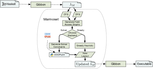
Figure 7: The overall pipeline of Marmoset.

The Gibbon front-end uses standard whole-program compilation and monomorphization techniques [7] to lower input programs into a first-order, monomorphic IR ($\lambda_{M}$). Gibbon performs location inference on this IR to convert it into a LoCal program, which has regions and locations, essentially, buffers and pointer arithmetic. Then a big middle section of the compiler is a series of LoCal $\rightarrow$ LoCal compiler passes that perform various transformations. Finally, it generates C code. Our extension operates towards the front-end of the compiler, on $\lambda_{M}$. We closely follow the design described in Section 3 to construct the control-flow graph and field-access graph, and use the standard Haskell graph library in our implementation.

To solve the constraints, we use IBM’s DOCPLEX (Decision Optimization CPLEX), because its API allows high level modelling such as logical expressions like implications, negations, logical AND etc. with relatively low overhead. Unfortunately, there isn’t a readily available Haskell library that can interface with DOCPLEX. Thus, we use it via its library bindings available for Python. Specifically, we generate a Python program that feeds the constraints to DOCPLEX and outputs an optimum field ordering to the standard output, which Marmoset reads and parses, and then reorders the fields accordingly.

5 Evaluation

We evaluate Marmoset on three applications. First is a pair of microbenchmarks: a list length function (Section 5.2.1) and a logical expression evaluator (Section 5.2.2). Second is a small library of operations with binary trees (Section 5.3). Third is a blog management software based on the BlogList example from the Sections 2–3 (Section 5.4). Besides the run times, we take a closer look at how Marmoset affects cache behavior (Section 5.5) and compile times (Section 10).

We detail the impact of various datatype layouts on the performance. As the baseline, we use Gibbon, the most closely related prior work. We also compare Marmoset with MLton (Section 5.4.5). For each benchmark, we run 99 iterations and report the run-time mean, median and the 95% confidence interval.

5.1 Experimental Setup

We run our benchmarks on a server-class machine with 64 CPUs, each with two threads. The CPU model is AMD Ryzen Threadripper 3990X with 2.2 GHz clock speed. The L1 cache size is 32 KB, L2 cache size is 512 KB and L3 cache size is 16 MB. We use Gibbon’s default C backend and call GCC 10.2.0 with -O3 to generate binaries.

5.2 Micro Benchmarks

We use two microbenchmarks to explore specific performance penalties imposed by a sub-optimal data layout.

5.2.1 Computing the length of a linked-list

This benchmark demonstrates the cost of de-referencing memory addresses which are not present in the cache. It uses the linked list datatype:

⬇

data List = Nil $\mid$ Cons Content List

If each element of the list is constructed using Cons, the traversal has to de-reference a pointer—to jump over the content—each time to access the tail of the list. This is an expensive operation, especially if the target memory address is not present in the cache. In contrast, if the Content and List fields were swapped, then to compute the length, the program only has to traverse $n$ bytes for a list of length $n$—one byte per Cons tag—which is extremely efficient. Essentially, Marmoset transforms program to use the following datatype, while preserving its behavior:

⬇

data List' = Nil' $\mid$ Cons' List' Content

In our experiment, the linked list is made of 3M elements and each element contains an instance of the Pandoc Inline datatype that occupies roughly 5KB. As seen in table 1(a), the performance of the list constructed using the original List is $\sim$60$\times$ worse than the performance with the Marmoset-optimized, flipped layout. Not only does List have poor data locality and cache behavior, but it also has to execute more instructions to de-reference the pointer. Both M_greedy and M_solver choose the flipped layout List'.

Table 1: Mean, Median and 95% confidence interval (ub, lb) for different layouts when compiled with Gibbon. The last two columns show the runtime for the layout chosen by M_greedy and M_solver. The numbers in Blue correspond to the lowest running time and the numbers in Red correspond to the highest running time. Legend: l - left subtree, r - right subtree of the mono tree.

(a) List length run times in milliseconds (ms)

	Gibbon				Marmoset
	List		List’		Mgreedy		Msolver
Mean	60.731		1.052		0.981		0.994
Median	60.730		1.017		0.978		0.979
ub	60.737		1.078		0.990		1.022
lb	60.725		1.025		0.973		0.964

(b) Logical expression evaluator run times in seconds (s)

	Gibbon				Marmoset
	lr		rl		Mgreedy		Msolver
Mean	$4.372\,658\,620\,370\,371$		$6.669\,544\,222\,222\,224$		$3.600\,981\,037\,037\,037$		$3.594\,482\,435\,185\,185$
Median	$4.313\,438$		$6.625\,107$		$3.534\,958$		$3.543\,093\,500\,000\,000\,3$
ub	$4.403\,732\,645\,795\,353$		$6.693\,175\,524\,408\,939\,5$		$3.648\,194\,996\,569\,051$		$3.635\,610\,184\,890\,118$
lb	$4.341\,584\,594\,945\,388$		$6.645\,912\,920\,035\,508$		$3.553\,767\,077\,505\,023$		$3.553\,354\,685\,480\,252$

(c) Rightmost tree runtime statistics in nano seconds (ns)

	Gibbon				Marmoset
	lr		rl		Mgreedy		Msolver
Mean	383.2		318.1		312.2		315.4
Median	360.0		300.0		300.0		300.0
ub	404.5		328.9		321.1		327.1
lb	362.4		307.2		303.4		303.8

5.2.2 Short-circuiting logical And/Or operators

These microbenchmarks operate over a synthetically generated, balanced syntax-tree with a height of 30. The intermediate nodes can be one of Not, Or, or And, selected at random, and the leaves consist of booleans wrapped in a Val. The evaluator function evaluates the expression tree and performs short circuiting for expressions like and and or in the expression tree. We measure the performance of this evaluator function by changing the order of the left and right subtrees. The syntax-tree datatype is defined as follows:

⬇

data Exp = Val Bool $\mid$ Not Exp $\mid$ Or Exp Exp $\mid$ And Exp Exp

Since the short circuiting evaluates from left to right order of the Exp, changing the order of the left and right subtrees would affect the performance of the traversal. As can be seen in table 1(b), the layout where the left subtree is serialized before the right subtree results in better performance compared to the tree where the the right subtree is serialized before the left one. This is as expected since in the latter case, the traversal has to jump over the right subtree serialized before the left one in order to evaluate it first and then depending on the result of the left subtree possibly jump back to evaluate the right subtree. This results in poor spatial locality and hence worse performance. M_greedy and M_solver are able to identify the layout transformations that would give the best performance, which matches the case where the left subtree is serialized before the right subtree. Table 1(b) shows the performance results.

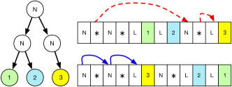
Figure 8: Rightmost: access patterns for, left-to-right (top) and right-to-left (bottom) serializations

5.3 Binary Tree benchmarks

We evaluate Marmoset on a few binary tree benchmarks. These include adding one to all values stored in the internal nodes of the tree, exponentiation on integers stored in internal nodes, copying a tree and getting the right-most leaf value in the tree. For the first three benchmarks, the tree representation we use is:

⬇

data Tree = Leaf $\mid$ Node Int Tree Tree

For right-most, the tree representation we use is:

⬇

data Tree = Leaf Int $\mid$ Node Tree Tree

5.3.1 Add one tree

This benchmark takes a full binary tree and increments the values stored in the internal nodes of the tree. We show the performance of an aligned preorder, inorder and postorder traversal in addition to a misaligned preorder and postorder traversal of the tree. Aligned traversals are ones where the data representation exactly matches the traversal order, for instance, a preorder traversal on a preorder representation of the tree. A misaligned traversal order is where the access patterns of the traversal don’t match the data layout of the tree. For instance, a postorder traversal on a tree serialized in preorder. Table 2 shows the performance numbers. M_solver picks the aligned postorder traversal order which is best performing. It makes the recursive calls to the left and right children of the tree first and increments the values stored in the internal nodes once the recursive calls return. The tree representation is also changed to a postorder representation with the Int placed after the left and right children of the tree. This is in part due to the structure of arrays effect, as the Int are placed closer to each other. M_greedy on the other hand picks the aligned preorder traversal because of its greedy strategy which prioritizes placing the Int before the left and right subtree. The tree depth was set to 27. At this input size, the Misaligned_post traversal failed due to memory errors. We see significant slowdowns with Misaligned_pre, $\sim$35$\times$ slower, because of the skewed access patterns of the traversal.

Table 2: Binary Tree benchmarks runtime statistics in seconds (s). Misaligned_pre– A post order traversal on a pre order layout of the tree. Misaligned_post– A pre order traversal on a post order layout of the tree. Aligned_pre– A pre order traversal on a pre order layout of the tree. Aligned_in– An in order traversal on an in order layout of the tree. Aligned_post– A post order traversal on a post order layout of the tree.

Gibbon

Marmoset

Misalignedpre

Misalignedpost

Alignedpre

Alignedin

Alignedpost

Mgreedy

Msolver

Add One Tree

Mean

45.506

memory error

$1.318\,870\,740\,740\,740\,7$

$1.327\,467\,398\,148\,148\,4$

$1.290\,646\,222\,222\,222\,4$

$1.318\,915\,222\,222\,222\,2$

$1.278\,920\,282\,828\,282\,4$

Median

45.507

memory error

$1.291\,547\,5$

$1.301\,803$

$1.288\,307$

$1.291\,284\,5$

$1.275\,409$

ub

45.661

memory error

$1.334\,508\,271\,008\,376$

$1.342\,853\,017\,459\,503$

$1.296\,121\,611\,091\,341\,6$

$1.334\,694\,924\,488\,772\,7$

$1.284\,846\,871\,407\,015\,6$

lb

45.351

memory error

$1.303\,233\,210\,473\,105\,5$

$1.312\,081\,778\,836\,793\,8$

$1.285\,170\,833\,353\,103\,1$

$1.303\,135\,519\,955\,671\,8$

$1.272\,993\,694\,249\,549\,2$

Exponentiation Tree

Mean

45.520

memory error

$1.338\,833\,731\,481\,481\,8$

$1.340\,895\,601\,851\,852$

$1.296\,339\,515\,151\,515\,1$

$1.336\,237\,537\,037\,037\,2$

$1.294\,804\,525\,252\,525$

Median

45.567

memory error

$1.312\,967\,5$

$1.314\,778\,5$

$1.293\,376$

$1.310\,292$

$1.291\,829$

ub

45.702

memory error

$1.354\,349\,493\,420\,148\,8$

$1.356\,565\,502\,024\,642$

$1.301\,961\,583\,230\,177\,4$

$1.352\,130\,068\,835\,353\,5$

$1.300\,631\,257\,753\,884\,3$

lb

45.338

memory error

$1.323\,317\,969\,542\,814\,8$

$1.325\,225\,701\,679\,062$

$1.290\,717\,447\,072\,852\,9$

$1.320\,345\,005\,238\,721$

$1.288\,977\,792\,751\,165\,9$

Copy Tree

Mean

45.524

memory error

$1.312\,177\,046\,296\,296$

$1.323\,082\,518\,518\,518\,7$

$1.281\,644\,191\,919\,191\,9$

$1.311\,649\,712\,962\,962\,7$

$1.278\,667\,242\,424\,242\,5$

Median

45.529

memory error

$1.286\,019\,5$

$1.296\,986\,5$

$1.278\,153$

$1.284\,783$

$1.276\,03$

ub

45.673

memory error

$1.327\,728\,808\,958\,863$

$1.338\,750\,685\,128\,81$

$1.287\,317\,967\,848\,180\,5$

$1.327\,481\,317\,169\,239\,7$

$1.284\,358\,794\,308\,634\,3$

lb

45.374

memory error

$1.296\,625\,283\,633\,729$

$1.307\,414\,351\,908\,227\,3$

$1.275\,970\,415\,990\,203\,2$

$1.295\,818\,108\,756\,685\,8$

$1.272\,975\,690\,539\,850\,6$

5.3.2 Exponentiation Tree

This traversal does exponentiation on the values stored in the internal nodes of the tree. It is more computationally intensive than incrementing the value. We raise the Int to a power of 10 on a tree of depth 27. Table 2 shows the performance of the different layout and traversal orders. M_solver picks the Aligned_post representation which is the best performing, whereas M_greedy picks the Aligned_pre representation.

5.3.3 Copy Tree

Copy-tree takes a full binary tree and makes a fresh copy of the tree in a new memory location. We use a tree of depth 27 in our evaluation. Table 2 shows the performance of different layout and traversal orders. We see that Aligned_post traversal performs the best. Indeed, M_solver picks the Aligned_post representation, whereas, M_greedy chooses the Aligned_pre representation.

5.3.4 Rightmost

This traversal does recursion on the right child of the tree and returns the Int value stored in the right-most leaf of the tree. Figure 8 shows an example of a tree with two different serializations of the tree: left-to-right (top) and right-to-left (bottom). The right-to-left serialization is more efficient because the constant-step movements (blue arrows) are usually more favorable than variable-step ones (red arrows) on modern hardware. Both M_solver and M_greedy pick the right-to-left serialization, and Table 1(c) shows that this choice performs better in the benchmark.

5.4 Blog Software Case Study

The Blog software case study serves as an example of a realistic benchmark, representing a sample of components from a blog management web service. The main data structure is a linked list of blogs where each blog contains fields such as header, ID, author information, content, hashtags and date. The fields are a mix of recursive and non-recursive datatypes. For instance, Content is a recursive type (the Pandoc Block type), but Author is a single string wrapped in a data constructor. One possible permutation of fields in the blog is:

⬇

data Blogs = Empty$\mid$HIADCTB Header Id Author Date Content HashTags Blogs

We evaluate Marmoset’s performance using three different traversals over a list of blogs. Overall, these traversals only use three fields: Content and Tags, and the tail of the linked-list, Blogs. The fields used by each individual traversal are referred as active fields and the rest are referred as passive fields, and we specify these per-traversal in the following. In Table 3 we report the performance of all six layouts obtained by permuting the order of these three fields, and two additional layouts (Columns 1 and 2). The column names are indicative of the order of fields used. For example, the column hiadctb reports numbers for a layout where the fields are ordered as: Header, Id, Author, Date, Content, HashTags, and Blogs (the tail of the list). We use Gibbon to gather these run times. The second to last and the last two columns show the run times of these traversals using Marmoset’s greedy and solver based optimization. The layout it picks is tailored to each individual traversal, so we specify it per-traversal next.

Table 3: Runtime statistics in seconds (s) for different blog traversals for a subset permutation of different layouts when compiled with Gibbon. Legend: h - Header, t - HashTags, b - Blogs, i - TagID, c - Content, a - Author, d - Date.

Gibbon

Marmoset

hiadctb

ctbhiad

tbchiad

tcbhiad

btchiad

bchiadt

cbiadht

Mgreedy

Msolver

Filter Blogs

Mean

$0.236\,865\,663\,888\,888\,83$

$0.223\,626\,064\,814\,814\,84$

$0.059\,331\,834\,537\,037\,04$

$0.255\,070\,140\,740\,740\,75$

$0.275\,882\,487\,037\,037\,05$

$0.287\,819\,479\,629\,629\,6$

$0.202\,519\,890\,740\,740\,75$

$0.067\,286\,970\,740\,740\,75$

0.071

Median

$0.233\,412$

$0.216\,983\,2$

$0.056\,234\,04$

$0.252\,306\,55$

$0.272\,412\,75$

$0.283\,701\,6$

$0.197\,381\,5$

$0.064\,556\,175$

0.065

ub

$0.238\,397\,515\,974\,954\,32$

$0.225\,874\,655\,240\,960\,31$

$0.061\,175\,230\,363\,156\,77$

$0.256\,384\,776\,097\,342\,45$

$0.277\,771\,733\,387\,891\,24$

$0.289\,606\,594\,491\,849\,1$

$0.205\,262\,877\,284\,320\,4$

$0.068\,804\,973\,013\,006\,71$

$0.074\,084\,687\,492\,241\,15$

lb

$0.235\,333\,811\,802\,823\,34$

$0.221\,377\,474\,388\,669\,37$

$0.057\,488\,438\,710\,917\,31$

$0.253\,755\,505\,384\,139\,05$

$0.273\,993\,240\,686\,182\,86$

$0.286\,032\,364\,767\,410\,1$

$0.199\,776\,904\,197\,161\,1$

$0.065\,768\,968\,468\,474\,78$

$0.068\,095\,031\,211\,462\,54$

Emph Content

Mean

$0.676\,896\,492\,592\,592\,5$

$0.645\,011\,936\,111\,111\,2$

$1.252\,170\,555\,555\,555\,6$

$0.661\,521\,869\,444\,444\,4$

$1.247\,634\,222\,222\,222$

$1.269\,061\,333\,333\,333\,4$

$0.483\,459\,769\,444\,444\,4$

$0.481\,856\,937\,037\,037$

0.648

Median

$0.664\,633\,9$

$0.629\,717\,75$

$1.247\,218$

$0.647\,435\,200\,000\,000\,1$

$1.246\,326$

$1.271\,372$

$0.464\,856\,65$

$0.463\,742\,650\,000\,000\,03$

0.646

ub

$0.684\,214\,375\,971\,199$

$0.653\,480\,881\,482\,957\,2$

$1.259\,318\,002\,043\,365\,2$

$0.669\,605\,509\,375\,354\,8$

$1.253\,413\,298\,510\,475$

$1.276\,522\,720\,510\,881\,8$

$0.494\,038\,204\,786\,560\,5$

$0.492\,572\,263\,400\,033\,85$

$0.650\,716\,151\,913\,629\,2$

lb

$0.669\,578\,609\,213\,986$

$0.636\,542\,990\,739\,265\,1$

$1.245\,023\,109\,067\,746$

$0.653\,438\,229\,513\,533\,9$

$1.241\,855\,145\,933\,969\,3$

$1.261\,599\,946\,155\,785$

$0.472\,881\,334\,102\,328\,3$

$0.471\,141\,610\,674\,040\,2$

$0.645\,128\,504\,652\,027\,1$

Tag Search

Mean

$2.032\,400\,527\,777\,778$

$2.017\,655\,231\,481\,481$

$2.768\,484\,333\,333\,333\,3$

$1.716\,654\,833\,333\,333\,4$

$2.802\,108\,222\,222\,222$

$2.809\,880\,222\,222\,222$

$1.857\,133\,740\,740\,740\,7$

$1.801\,490\,703\,703\,703\,3$

1.733

Median

$1.993\,22$

$1.976\,430\,5$

$2.766\,269$

$1.661\,759$

$2.801\,901$

$2.809\,493$

$1.804\,684$

$1.746\,745\,499\,999\,999\,8$

1.724

ub

$2.056\,570\,170\,215\,674$

$2.042\,352\,241\,875\,830\,6$

$2.773\,769\,727\,132\,014\,8$

$1.749\,551\,172\,566\,805\,6$

$2.805\,736\,222\,347\,774$

$2.811\,850\,435\,449\,460\,7$

$1.888\,528\,756\,113\,495\,4$

$1.834\,483\,954\,542\,924\,6$

$1.746\,409\,750\,718\,698\,2$

lb

$2.008\,230\,885\,339\,882$

$1.992\,958\,221\,087\,131\,5$

$2.763\,198\,939\,534\,652$

$1.683\,758\,494\,099\,861\,1$

$2.798\,480\,222\,096\,67$

$2.807\,910\,008\,994\,983\,6$

$1.768\,497\,452\,864\,482\,1$

$1.719\,111\,522\,008\,574$

$1.633\,349\,537\,273\,928\,6$

5.4.1 FilterBlogs

This traversal filters the list of blogs and only retains those which contain the given hash-tag in their HashTags field. Since Blogs, Content, and HashTags are recursive fields, changing their layout should represent greater differences in performance. The active fields for this traveral are HashTags and Blogs. Theoretically, the performance of this traversal is optimized when the HashTags field is serialized before Blogs on account of the first access to HashTags in the traversal. This is confirmed in practice with the layout tbchiad being the fastest. The access to HashTags comes first since its serialized first in memory and once HashTags is fully traversed, the traversal can access blogs in an optimal manner without unnecessary movement in the packed buffer.

Indeed, the layout chosen by Marmoset puts HashTags first followed by Blogs. The order of the rest of the fields remains unchanged compared to the source program, but this has no effect on performance since they are passive fields. As shown in Table 3, the performance of the layout chosen by Marmoset is similar to the layout tbchiad when compiled with Gibbon. Both M_solver and M_greedy pick the layout tbhiadc when compiled from the initial layout hiadctb.

5.4.2 EmphContent

This traversal takes a keyword and a list of blogs as input. It then searches the content of each blog for the keyword and emphasizes all its occurrences if present. If the keyword isn’t present, the content remains unchanged. The active fields in this traversal are Content and Blogs. Therefore, based on the access pattern (Content accessed before Blogs), the layout with the best performance should place Content first followed by Blogs. Indeed, the layout with the best performance when compiled with Gibbon is cbiadht. The layout that M_solver chooses prioritizes the placement of Blogs before Content. It subsequently changes the traversal to recurse on the blogs first and then emphasize content. The other passive fields are all placed afterwards. The layout chosen by M_solver is bchiadt, whereas the layout chosen by M_greedy is cbhiadt when compiled from the initial layout hiadctb. Table 3 shows the performance of all the layouts for this traversal. The performance of M_greedy and M_solver differ because data constructors not shown differ in their layout choices.

5.4.3 TagSearch

This traversal takes a keyword and a list of blogs as input. It looks for the presence of a keyword in the HashTags field. If it is present, it emphasizes this keyword in the Content, and leaves it unchanged otherwise. The layout that gives the best performance when compiled with Gibbon is tcbhiad. This is as expected based on the access patterns of the traversal which access HashTags followed by Content followed by Blogs. M_solver chooses the layout tbchiad which places HashTags, followed by Blogs, followed by Content and changes the traversal to recurse on Blogs first and later emphasize Content in the then branch. On the other hand, the layout chosen by M_greedy is tcbhiad when compiled from the initial layout hiadctb.

5.4.4 Globally optimizing multiple functions

We use Marmoset to globally optimize the three blog traversals we discussed above such that we pick one layout for all traversals that minimizes the overall runtime. Table 4 shows the runtime for a layout we compiled using Gibbon (hiadctb), M_solver (tbchiad) and M_greedy (tbchiad). We see that M_greedy and M_solver do a good job in reducing the traversal time globally. All the three traversals are run in a pipelined fashion sequentially. Although, M_solver does worse with TagSearch when run in a pipelined manner, it is actually better performing with M_solver when run alone as seen in table 3. Note that M_solver changes more that one data constructor based on the inlineable attribute that M_greedy does not. For instance, M_solver uses a packed Inline list in the Content with the tail serialized before Inline. Whereas, M_greedy uses a conventional packed list. In a pipelined execution of the traversals, although this helps reduce the runtime in the case of the content search traversal, it inadvertently increases the runtime in case of the tag search traversal due to a cache effect that can benefit from runtime information.

Table 4: Runtime in seconds for different blog traversals when we use Marmoset to globally optimize the data layout. The input parameters are different from the single function case.

(a) Filter Blogs

	Gibbon		Mgreedy		Msolver
Mean	$1.926\,918\,888\,888\,888\,8$		$0.101\,968\,213\,131\,313\,13$		$0.104\,246\,677\,777\,777\,77$
Median	$1.925\,58$		$0.101\,113\,4$		$0.102\,765\,9$
ub	$1.930\,799\,059\,311\,418\,2$		$0.102\,606\,986\,857\,571\,25$		$0.105\,125\,781\,081\,590\,64$
lb	$1.923\,038\,718\,466\,359\,5$		$0.101\,329\,439\,405\,055\,01$		$0.103\,367\,574\,473\,964\,9$

(b) Emph Content

	Gibbon		Mgreedy		Msolver
Mean	$1.582\,479\,656\,565\,656\,5$		$1.388\,232\,272\,727\,272\,7$		$1.325\,701\,141\,414\,141\,5$
Median	$1.578\,678$		$1.384\,18$		$1.320\,468$
ub	$1.589\,285\,432\,654\,959\,7$		$1.396\,201\,464\,419\,347\,4$		$1.336\,001\,926\,809\,490\,7$
lb	$1.575\,673\,880\,476\,353\,3$		$1.380\,263\,081\,035\,198$		$1.315\,400\,356\,018\,792\,3$

(c) Tag Search

	Gibbon		Mgreedy		Msolver
Mean	$2.186\,549\,565\,656\,565\,4$		$1.830\,526\,727\,272\,727\,5$		$2.356\,293\,929\,292\,929\,2$
Median	$2.182\,541$		$1.826\,959$		$2.351\,989$
ub	$2.193\,582\,984\,981\,658$		$1.838\,355\,525\,519\,980\,8$		$2.364\,621\,853\,531\,670\,8$
lb	$2.179\,516\,146\,331\,472\,7$		$1.822\,697\,929\,025\,474\,1$		$2.347\,966\,005\,054\,187\,7$

5.4.5 Comparison of Marmoset against MLton

We compare Marmoset’s performance to MLton, which compiles programs written in Standard ML, a strict language, to executables that are small with fast runtime performance.

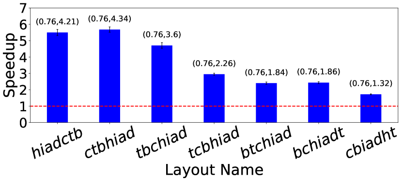
(a) Filter Blogs Traversal.

(b) Content Search Traversal.

(c) Tag Search Traversal.

Figure 9: Performance comparison of M_solver with MLton. The tuple on top of each bar shows the median runtime in seconds of M_solver followed by the corresponding layout when compiled with MLton.

Figure 9 shows the the speedup of Marmoset over MLton. As shown, the performance of Marmoset is better than MLton by significant margins for all the layouts and traversals. Since ADTs in MLton are boxed – even though native integers or native arrays are unboxed – such a behavior is expected because it adds more instructions (pointer de-referencing) and results in worse spatial locality.

5.5 Cache behavior

Table 5: PAPI performance counter statistics (average of 99 runs) for different blog traversals.

Gibbon

Marmoset

hiadctb

ctbhiad

tbchiad

tcbhiad

btchiad

bchiadt

cbiadht

Mgreedy

Msolver

Filter Blogs

Ins

$583\,007\,860.888\,888\,8$

$582\,007\,417.222\,222\,2$

$583\,006\,557.555\,555\,6$

$581\,007\,422.0$

$579\,006\,542.111\,111\,2$

$578\,007\,431.333\,333\,4$

$586\,007\,412.444\,444\,4$

$583\,006\,551.444\,444\,4$

$583\,006\,570.444\,444\,4$

Cycles

$989\,222\,808.888\,888\,8$

$959\,711\,380.111\,111\,2$

$285\,081\,123.888\,888\,9$

$1\,052\,921\,958.222\,222\,2$

$1\,200\,439\,241.333\,333\,3$

$1\,248\,215\,771.111\,111\,2$

$877\,792\,663.111\,111\,2$

$279\,146\,331.444\,444\,4$

$289\,017\,037.777\,777\,8$

L2 DCM

$11\,185\,155.333\,333\,334$

$11\,510\,078.222\,222\,222$

$938\,489.333\,333\,333\,4$

$13\,337\,049.333\,333\,334$

$12\,928\,602.222\,222\,222$

$13\,065\,840.0$

$7\,789\,525.777\,777\,778$

$889\,989.777\,777\,777\,8$

$874\,607.777\,777\,777\,8$

Content Search

Ins

$5\,845\,022\,229.888\,889$

$5\,834\,021\,360.444\,445$

$6\,776\,362\,325.666\,667$

$5\,841\,021\,767.888\,889$

$6\,779\,241\,706.444\,445$

$6\,779\,244\,615.888\,889$

$5\,837\,021\,292.777\,778$

$5\,837\,021\,295.333\,333$

$5\,837\,021\,366.222\,222$

Cycles

$2\,892\,647\,565.888\,889$

$2\,738\,456\,405.444\,444\,7$

$4\,272\,337\,912.0$

$2\,842\,427\,055.666\,666\,5$

$4\,340\,585\,270.333\,333$

$4\,291\,414\,051.555\,555\,3$

$2\,056\,621\,185.333\,333\,3$

$2\,061\,807\,292.666\,666\,7$

$2\,812\,417\,391.555\,555\,3$

L2 DCM

$12\,800\,140.0$

$10\,780\,195.333\,333\,334$

$20\,295\,265.222\,222\,224$

$13\,283\,107.333\,333\,334$

$20\,549\,853.111\,111\,112$

$20\,994\,551.666\,666\,668$

$7\,727\,582.888\,888\,889$

$7\,663\,269.0$

$10\,702\,561.555\,555\,556$

Tag Search

Ins

$22\,490\,860\,539.777\,78$

$22\,487\,260\,185.555\,557$

$23\,043\,358\,250.333\,332$

$22\,487\,260\,291.333\,332$

$23\,043\,009\,879.0$

$23\,041\,811\,630.222\,22$

$22\,488\,060\,134.777\,78$

$22\,487\,659\,963.444\,443$

$22\,487\,659\,965.0$

Cycles

$8\,587\,261\,902.555\,555$

$8\,593\,729\,939.888\,89$

$9\,609\,104\,561.222\,221$

$7\,288\,093\,434.666\,667$

$9\,607\,367\,711.666\,666$

$9\,748\,577\,539.111\,11$

$7\,883\,183\,997.666\,667$

$7\,609\,921\,682.888\,889$

$7\,568\,236\,436.222\,222$

L2 DCM

$20\,227\,011.777\,777\,776$

$20\,621\,886.333\,333\,332$

$39\,956\,792.444\,444\,45$

$10\,612\,695.222\,222\,222$

$28\,602\,975.777\,777\,776$

$26\,479\,819.222\,222\,224$

$16\,392\,591.777\,777\,778$

$12\,885\,043.444\,444\,444$

$12\,753\,814.333\,333\,334$

The results from earlier sections demonstrate that Marmoset’s layout choices improve run-time performance. This section investigates why performance improves. The basic premise of Marmoset’s approach to layout optimization is to concentrate on minimizing how often a traversal needs to backtrack or skip ahead while processing a buffer. By minimizing this jumping around, we expect to see improvements from two possible sources. First, we expect to see an improvement in instruction counts, as an optimized layout should do less pointer chasing. Second, we expect to see an improvement in L2 and L3 cache utilization: both fewer misses (due to improved spatial locality and prefetching) and fewer accesses (due to improved locality in higher level caches).

Table 5 shows that our main hypothesis is borne out and the optimal layout has fewer L2 data cache misses: a better layout promotes better locality. Interestingly, we do not observe a similar effect for instruction count. While different layouts differ in instruction counts, the difference is slight. We suspect this light effect of a better layout may be due to Gibbon’s current implementation, which often dereferences pointers even if a direct access in the buffer would suffice.

5.6 Tradeoffs between Marmoset’s solver and greedy optimization

To understand the difference between the layout chosen by M_solver and M_greedy we now take a closer look at the tag search traversal shown in Table 3. Here, both versions choose two different layouts with different performance implications. M_solver chooses the layout tbchiad whereas M_greedy chooses the layout tcbhiad. The mechanics of why can be explained using our running example (Figure 1) which is essentially a simplified version of the traversal shown in the evaluation. Figure 5(b) shows the access graph for this traversal. M_solver generates constraints outlined in Section 3.6 that lead to the layout tbchiad. On the other hand, M_greedy starts at the root node of the graph and greedily chooses the next child to traverse. The order in which nodes of the graph are visited fixes the order of fields in the data constructor. In this case, the root node is HashTags which makes it the first field in the greedy layout, next, the greedy heuristic picks the Content field making it the second field and finally followed by the BlogList field.

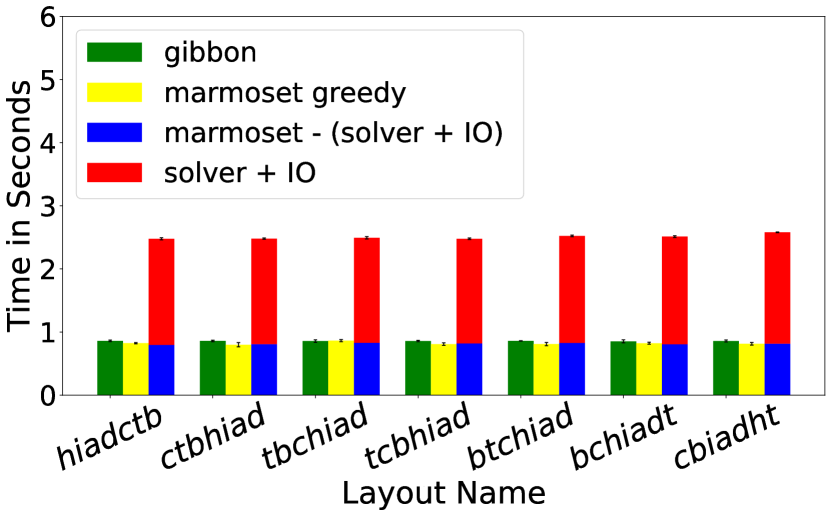
(a) Filter blogs traversal

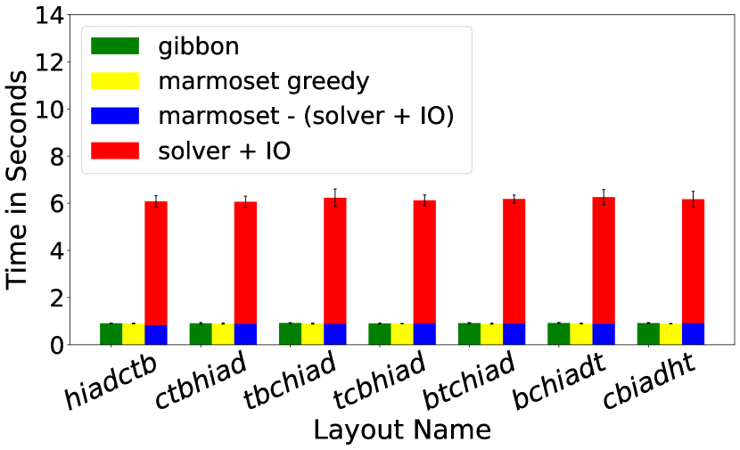
(b) Content Search traversal

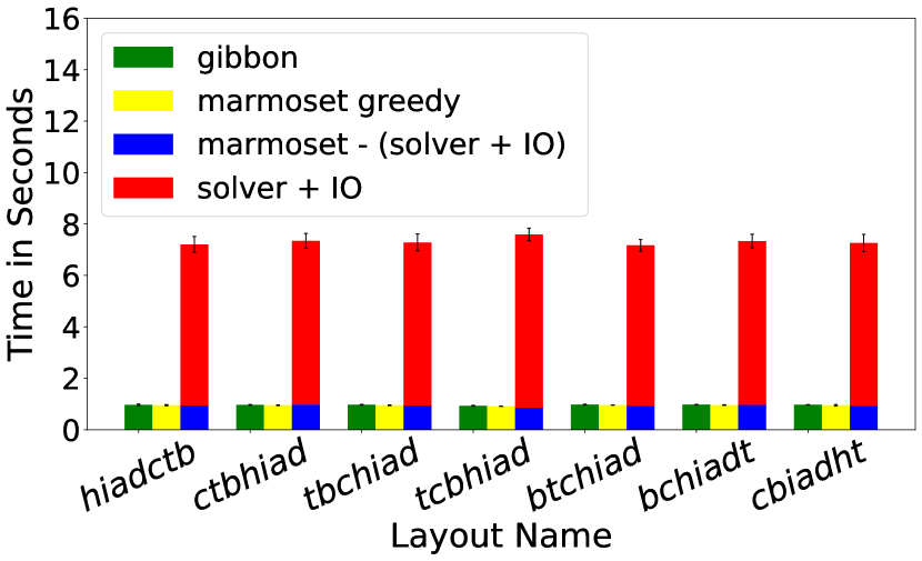
(c) Tag Search traversal

Figure 10: Average compile times (99 runs) in (s) for different layouts and traversal combinations when compiled with Gibbon and when optimized by M_greedy and M_solver. The bar in Blue is the time for M_solver after subtracting the time for solver IO and the bar in Red is the time taken to do the IO call to the DOCPLEX solver. The total compile time for M_solver includes the time for doing the CFG analysis, generating the access graph, the solver time, reordering the datatype and repairing the code, The majority of which is added by the solver IO.

We show the compile times in Figure 10 for different layout and traversal combinations when compiled with Gibbon, M_greedy and M_solver respectively as a measure of relative costs. The compile times for M_solver include the time to generate the control flow graph, the field access graph, the solver time and the time to re-order the datatype in the code. The solver times are in the order of the number of fields in a data constructor and not the program size. Hence, the solver adds relatively low overhead. Since the compiler does an IO call to the python solver, there is room for improvement in the future to lower these times. For instance, we could directly perform FFI calls to the CPLEX solver by lowering the constraints to C code. This would be faster and safer than the current implementation. In addition, during the global optimization, we call the solver on each data constructor as of the moment, we could further optimize this by sending constraints for all data constructors at once and doing just one solver call.

Although the cost of Marmoset’s solver based optimization is higher that the greedy approach, it is a complementary approach which may help the user find a better layout at the cost of compile time. On the other hand, if the user wishes to optimize for the compile time, they should use the greedy heuristic.

5.7 Discussion: Scale of Evaluation

Marmoset’s approach for finding the best layout for densely presented data is language agnostic, but the evaluation has to be language specific. Hence, we implemented the approach inside a most-developed (to our knowledge) compiler supporting dense representations of recursive datatypes, the Gibbon compiler. Our evaluation is heavily influenced by this.

At the time of writing, the scale of evaluation is limited by a number of Gibbon-related restrictions. Gibbon is meant as a tree traversal accelerator [24] and its original suite of benchmarks served as a basis and inspiration for evaluation of Marmoset. “Big” end-to-end projects (e.g. compilers, web servers, etc.) have not been implemented in Gibbon and, therefore, are out of reach for us. If someone attempted to implement such a project using Gibbon, they would have to extend the compiler to support many realistic features: modules, FFI, general I/O, networking. Alternatively, one could integrate Gibbon into an existing realistic compiler as an optimization pass or a plugin. For instance, the Gibbon repository has some preliminary work for integrating as a GHC plugin, but it is far from completion. In any case, the corresponding effort is simply too big. Overall, the current Marmoset evaluation shows that our approach is viable.

6 Discussion

Marmoset allows the user to provide optional manual constraints on the layout as either relative or absolute constraints through ANN annotation pragmas. The relative constraint allows the user to specify if a field A comes immediately after field B. The absolute constraint specifies an exact index in the layout for a field. Such pragmas may be beneficial if the user requires a specific configuration over data types or has information about performance bottlenecks.

Although the performance optimization is currently statically driven, there are many avenues for future improvement. For instance, we can get better edges weights for the access graphs using dynamic profiling techniques. The profiling can be quite detailed, for instance, which branch in a function is more likely, which function takes the most time overall in a global setting (the optimization would bias the layout towards that function), how does a particular global layout affect the performance in case of a pipeline of functions.

We could also look at a scenario where we optimize each function locally and use “shim” functions that copy one layout to another (the one required by the next function in the pipeline). Although the cost of copying may be high, it warrants further investigation. Areas of improvement purely on the implementation side include optimizing whether Marmoset dereferences a pointer to get to a field or uses the end-witness information as mentioned in section 2. Lesser pointer dereferencing can lower instruction counts and impact performance positively. We would also like to optimize the solver times as mentioned in 10.

We envision that the structure of arrays effect that we discovered may help with optimizations such as vectorization, where the performance can benefit significantly if the same datatype is close together in memory. Regardless, through the case studies, we see that Marmoset shows promise in optimizing the layout of datatypes and may open up the optimization space for other complex optimizations such as vectorization.

7 Related Work

7.1 Cache-conscious data

Chilimbi and Larus [6] base on an object-oriented language with a generational garbage collector, which they extend with a heuristic for copying objects to the TO space. Their heuristic uses a special-purpose graph data structure, the object affinity graph, to identify when groups of objects are accessed by the program close together in time. When a given group of objects have high affinity in the object affinity graph, the collector is more likely to place them close together in the TO space. As such, a goal of their work and ours is to achieve higher data-access locality by carefully grouping together objects in the heap. However, a key difference from our work is that their approach bases its placement decisions on an object-affinity graph that is generated from profiling data, which is typically collected online by some compiler-inserted instrumentation. The placement decisions made by our approach are based on data collected by static analysis of the program. Such an approach has the advantage of not depending on the output of dynamic profiling, and therefore avoids the implementation challenges of dynamic profiling. A disadvantage of not using dynamic profiling is that the approach cannot adapt to changing access patterns that are highly input specific. We leave open for future work the possibility of getting the best of both approaches.

Chilimbi et al. [4] introduce the idea of hot/cold splitting of a data structure, where elements are categorized as being “hot” if accessed frequently and “cold” if accessed inferquently. This information is obtained by profiling the program. Cold fields are placed into a new object via an indirection and hot fields remain unchanged. In their approach, at runtime, there is a cache-concious garbage collector [6] that co-locates the modified object instances. This paper also suggests placing fields with high temporal affinity within the same cache block. For this they recommend bbcache, a field recommender for a data structure. bbcache forms a field affinity graph which combines static information about the source location of structure field accesses with dynamic information about the temporal ordering of accesses and their access frequency.

Chilimbi et al. [5] propose two techniques to solve the problem of poor reference locality.

• ccmorph: This works on tree-like data structures, and it relies on the programmer making a calculated guess about the safety of the operation on the tree-like data structure. It performs two major optimizations: clustering and coloring. Clustering take a the tree like data structure and attempts to pack likely to be accessed elements in the structure within the same cache block. There are various ways to pack a subtree, including clustering $k$ nodes in a subtree together, depth first clustering, etc. Coloring attempts to map simultaneously accessed data elements to non-conflicting regions of the cache.

• ccmalloc: This is a memory allocator similar to malloc which takes an additional parameter that points to an existing data structure element which is likely accessed simultaneously. This requires programmer knowledge and effort in recognizing and then modifying the code with such a data element. ccmalloc tries to allocate the new data element as close to the existing data as possible, with the initial attempt being to allocate in the same cache block. It tries to put likely accessed elements on the same page in an attempt to improve TLB performance.

Franco et al. [13, 14] suggest that the layout of a data structure should be defined once at the point of initialization, and all further code that interacts with the structure should be “layout agnostic”. Ideally, this means that performance improvements involving layout changes can be made without requiring changes to program logic. To achieve this, classes are extended to support different laouts, and types carry layout information—code that operates on objects may be polymorphic over the layout details.

7.2 Data layout description and binary formats

Chen et al. [3] propose a data layout description framework Dargent, which allows programmers to specify the data layout of an ADT. It is built on top of the Cogent language [19], which is a first order polymorphic functional programming language. Dargent targets C code and provides proofs of formal correctness of the compiled C code with respect to the layout descriptions. Rather than having a compiler attempting to determine an efficient layout, their focus is on allowing the programmer to specify a particular layout they want and have confidence in the resulting C code.

Significant prior work went into generation of verified efficient code for interacting with binary data formats (parsing and validating). For example, EverParse [21] is a framework for generating verified parsers and formatters for binary data formats, and it has been used to formally verify zero-copy parsers for authenticated message formats. With Narcissus [9], encoders and decoders for binary formats could be verified and extracted, allowing researchers to certify the packet processing for a full internet protocol stack. Other work [22] has also explored the automatic generation of verified parsers and pretty printers given a specification of a binary data format, as well as the formal verification of a compiler for a subset of the Procotol Buffer serialization format [25].

Back [1] demonstrates how a domain-specific language for describing binary data formats could be useful for generating validators and for easier scripting and manipulation of the data from a high-level language like Java. [18] introduce Packet Types for programming with network protocol messages and provide language-level support for features commonly found in protocol formats like variable-sized and optional fields.

Hawkins et al. [15] introduce RELC, a framework for synthesizing low-level C++ code from a high-level relational representation of the code. The user describes and writes code that represents data at a high level as relations. Using a decomposition of the data that outlines memory representation, RELC synthesizes correct and efficient low-level code.

Baudon et al. [2] introduce the Ribbit DSL, which allows programmers to describe the layout of ADTs that are monomorphic and immutable. Ribbit provides a dual view on ADTs that allows both a high-level description of the ADT that the client code follows and a user-defined memory representation of the ADT for a fine-grained encoding of the layout. Precise control over memory layout allows Ribbit authors to develop optimization algorithms over the ADTs, such as struct packing, bit stealing, pointer tagging, unboxing, etc. Although this approach enables improvements to layout of ADTs, it is different from Marmoset’s: Ribbit focuses on manually defining low-level memory representation of the ADT whereas Marmoset automatically optimizes the high-level layout (ordering of fields in the definition ADT) relying on Gibbon for efficient packing of the fields. While Ribbit invites the programmer to encode their best guess about the optimal layout, Marmoset comes up with such layout by analysing access patterns in the source code.

7.3 Memory layouts

Early work on specifications of memory layouts was explored in various studies of PADS, a language for describing ad hoc data-file formats [10, 11, 17].

Lattner and Adve [16] introduce a technique for improving the memory layout of the heap of a given C program. Their approach is to use the results of a custom static analysis to enable pool allocation of heap objects. Such automatic pool allocation bears some resemblance to our approach, where we use region-based allocation in tandem with region inference, and thanks to static analysis can group fields of a given struct into the same pool, thereby improving locality in certain circumstances.

Floorplan [8] is a declarative language for specifying high-level memory layouts, implemented as a compiler which generates Rust code. The language has forms for specifying sizes, alignments, and other features of chunks of memory in the heap, with the idea that any correct state of the heap can be derived from the Floorplan specification. It was successfully used to eliminate 55 out of 63 unsafe lines of code (all of the unsafe code relating to memory safety) of the immix garbage collector.

8 Conclusions

This paper introduced Marmoset, which builds on Gibbon to generate efficient orders for Algebraic Datatypes. We observed that a fairly straightforward control-flow and data-flow analysis allows Marmoset to identify opportunities to place fields of a data constructor near each other in memory to promote efficient consecutive access to those fields. Because a given function might use many fields in many different ways, Marmoset adopts an approach of formulating the data layout problem as an ILP, with a cost model that assigns an abstract cost to a chosen layout. This ILP can be further constrained with user-provided layout guidelines. Armed with problem formulation, an off-the-shelf ILP solver allows Marmoset to generate minimal-(abstract)-cost layouts for algebraic datatypes. Marmoset then uses these layouts to synthesize a new ADT and prior work’s Gibbon compiler toolchain to lower the code into an efficient program that operates over packed datatypes with minimal pointer chasing.

We found, across a number of benchmarks, that Marmoset is able to effectively and consistently find the optimal data layout for a given combination of traversal function and ADT. We showed, experimentally, that Marmoset-optimized layouts significantly outperform not only Gibbon’s default layouts, but also GHC’s standard compiler.

References

- [1] Godmar Back. Datascript - a specification and scripting language for binary data. In Proceedings of the 1st ACM SIGPLAN/SIGSOFT Conference on Generative Programming and Component Engineering, GPCE ’02, page 66–77, Berlin, Heidelberg, 2002. Springer-Verlag.
- [2] Thaïs Baudon, Gabriel Radanne, and Laure Gonnord. Bit-stealing made legal: Compilation for custom memory representations of algebraic data types. Proc. ACM Program. Lang., 7(ICFP), aug 2023. doi:10.1145/3607858.
- [3] Zilin Chen, Ambroise Lafont, Liam O’Connor, Gabriele Keller, Craig McLaughlin, Vincent Jackson, and Christine Rizkallah. Dargent: A silver bullet for verified data layout refinement. Proc. ACM Program. Lang., 7(POPL), jan 2023. doi:10.1145/3571240.
- [4] Trishul M. Chilimbi, Bob Davidson, and James R. Larus. Cache-conscious structure definition. In Proceedings of the ACM SIGPLAN 1999 Conference on Programming Language Design and Implementation, PLDI ’99, page 13–24, New York, NY, USA, 1999. Association for Computing Machinery. doi:10.1145/301618.301635.
- [5] Trishul M. Chilimbi, Mark D. Hill, and James R. Larus. Cache-conscious structure layout. In Proceedings of the ACM SIGPLAN 1999 Conference on Programming Language Design and Implementation, PLDI ’99, page 1–12, New York, NY, USA, 1999. Association for Computing Machinery. doi:10.1145/301618.301633.
- [6] Trishul M. Chilimbi and James R. Larus. Using generational garbage collection to implement cache-conscious data placement. In Proceedings of the 1st International Symposium on Memory Management, ISMM ’98, page 37–48, New York, NY, USA, 1998. Association for Computing Machinery. doi:10.1145/286860.286865.
- [7] Adam Chlipala. An optimizing compiler for a purely functional web-application language. In Proceedings of the 20th ACM SIGPLAN International Conference on Functional Programming, ICFP 2015, pages 10–21, New York, NY, USA, 2015. ACM. URL: http://doi.acm.org/10.1145/2784731.2784741, doi:10.1145/2784731.2784741.
- [8] Karl Cronburg and Samuel Z. Guyer. Floorplan: Spatial layout in memory management systems. In Proceedings of the 18th ACM SIGPLAN International Conference on Generative Programming: Concepts and Experiences, GPCE 2019, page 81–93, New York, NY, USA, 2019. Association for Computing Machinery. doi:10.1145/3357765.3359519.
- [9] Benjamin Delaware, Sorawit Suriyakarn, Clément Pit-Claudel, Qianchuan Ye, and Adam Chlipala. Narcissus: Correct-by-construction derivation of decoders and encoders from binary formats. Proc. ACM Program. Lang., 3(ICFP), jul 2019. doi:10.1145/3341686.
- [10] Kathleen Fisher and Robert Gruber. Pads: A domain-specific language for processing ad hoc data. In Proceedings of the 2005 ACM SIGPLAN Conference on Programming Language Design and Implementation, PLDI ’05, page 295–304, New York, NY, USA, 2005. Association for Computing Machinery. doi:10.1145/1065010.1065046.
- [11] Kathleen Fisher and David Walker. The pads project: An overview. In Proceedings of the 14th International Conference on Database Theory, ICDT ’11, page 11–17, New York, NY, USA, 2011. Association for Computing Machinery. doi:10.1145/1938551.1938556.
- [12] Cormac Flanagan, Amr Sabry, Bruce F. Duba, and Matthias Felleisen. The essence of compiling with continuations. In Proceedings of the ACM SIGPLAN 1993 Conference on Programming Language Design and Implementation, PLDI ’93, page 237–247, New York, NY, USA, 1993. Association for Computing Machinery. doi:10.1145/155090.155113.
- [13] Juliana Franco, Martin Hagelin, Tobias Wrigstad, Sophia Drossopoulou, and Susan Eisenbach. You can have it all: Abstraction and good cache performance. In Proceedings of the 2017 ACM SIGPLAN International Symposium on New Ideas, New Paradigms, and Reflections on Programming and Software, Onward! 2017, page 148–167, New York, NY, USA, 2017. Association for Computing Machinery. doi:10.1145/3133850.3133861.
- [14] Juliana Franco, Alexandros Tasos, Sophia Drossopoulou, Tobias Wrigstad, and Susan Eisenbach. Safely abstracting memory layouts, 2019. URL: https://arxiv.org/abs/1901.08006, doi:10.48550/ARXIV.1901.08006.
- [15] Peter Hawkins, Alex Aiken, Kathleen Fisher, Martin Rinard, and Mooly Sagiv. Concurrent data representation synthesis. In Proceedings of the 33rd ACM SIGPLAN Conference on Programming Language Design and Implementation, PLDI ’12, page 417–428, New York, NY, USA, 2012. Association for Computing Machinery. doi:10.1145/2254064.2254114.
- [16] Chris Lattner and Vikram Adve. Automatic pool allocation for disjoint data structures. In Proceedings of the 2002 Workshop on Memory System Performance, MSP ’02, page 13–24, New York, NY, USA, 2002. Association for Computing Machinery. doi:10.1145/773146.773041.
- [17] Yitzhak Mandelbaum, Kathleen Fisher, David Walker, Mary Fernandez, and Artem Gleyzer. Pads/ml: A functional data description language. In Proceedings of the 34th Annual ACM SIGPLAN-SIGACT Symposium on Principles of Programming Languages, POPL ’07, page 77–83, New York, NY, USA, 2007. Association for Computing Machinery. doi:10.1145/1190216.1190231.
- [18] Peter J. McCann and Satish Chandra. Packet types: Abstract specification of network protocol messages. In Proceedings of the Conference on Applications, Technologies, Architectures, and Protocols for Computer Communication, SIGCOMM ’00, page 321–333, New York, NY, USA, 2000. Association for Computing Machinery. doi:10.1145/347059.347563.
- [19] Liam O’Connor, Christine Rizkallah, Zilin Chen, Sidney Amani, Japheth Lim, Yutaka Nagashima, Thomas Sewell, Alex Hixon, Gabriele Keller, Toby Murray, et al. Cogent: certified compilation for a functional systems language. arXiv preprint arXiv:1601.05520, 2016.
- [20] Chris Okasaki. Purely Functional Data Structures. Cambridge University Press, 1998.
- [21] Tahina Ramananandro, Antoine Delignat-Lavaud, Cédric Fournet, Nikhil Swamy, Tej Chajed, Nadim Kobeissi, and Jonathan Protzenko. Everparse: Verified secure zero-copy parsers for authenticated message formats. In Proceedings of the 28th USENIX Conference on Security Symposium, SEC’19, page 1465–1482, USA, 2019. USENIX Association.
- [22] Marcell van Geest and Wouter Swierstra. Generic packet descriptions: Verified parsing and pretty printing of low-level data. In Proceedings of the 2nd ACM SIGPLAN International Workshop on Type-Driven Development, TyDe 2017, page 30–40, New York, NY, USA, 2017. Association for Computing Machinery. doi:10.1145/3122975.3122979.
- [23] Michael Vollmer, Chaitanya Koparkar, Mike Rainey, Laith Sakka, Milind Kulkarni, and Ryan R. Newton. Local: A language for programs operating on serialized data. In Proceedings of the 40th ACM SIGPLAN Conference on Programming Language Design and Implementation, PLDI 2019, page 48–62, New York, NY, USA, 2019. Association for Computing Machinery. doi:10.1145/3314221.3314631.
- [24] Michael Vollmer, Sarah Spall, Buddhika Chamith, Laith Sakka, Chaitanya Koparkar, Milind Kulkarni, Sam Tobin-Hochstadt, and Ryan R. Newton. Compiling Tree Transforms to Operate on Packed Representations. In Peter Müller, editor, 31st European Conference on Object-Oriented Programming (ECOOP 2017), volume 74 of Leibniz International Proceedings in Informatics (LIPIcs), pages 26:1–26:29, Dagstuhl, Germany, 2017. Schloss Dagstuhl–Leibniz-Zentrum fuer Informatik. URL: http://drops.dagstuhl.de/opus/volltexte/2017/7273, doi:10.4230/LIPIcs.ECOOP.2017.26.
- [25] Qianchuan Ye and Benjamin Delaware. A verified protocol buffer compiler. In Proceedings of the 8th ACM SIGPLAN International Conference on Certified Programs and Proofs, CPP 2019, page 222–233, New York, NY, USA, 2019. Association for Computing Machinery. doi:10.1145/3293880.3294105.