The deceleration parameter in perturbed
Bianchi universes with a “tilt”

Abstract

Relative motion effects have long been known to “contaminate” the observations. In fact, when looking back to the history of astronomy, one finds a number of examples where relative motions have led to a gross misinterpretation of reality. Using relativistic cosmological perturbation theory it was shown that observers living inside bulk-flow domains that expand slightly slower than their surroundings, can have the illusion of cosmic acceleration, while the host universe is actually decelerating. This claim was originally based on studies of a perturbed tilted Einstein-de Sitter model, primarily for mathematical simplicity. Nevertheless, nothing really changed when the background universe was replaced by a Friedmann cosmology with nonzero pressure and spatial curvature. This raised the possibility that the peculiar-motion effect on the deceleration parameter, as measured locally by the bulk-flow observers, may be generic and independent of the specifics of the host universe. Here, we investigate this possibility, by extending the earlier studies to perturbed Bianchi cosmologies. We find that the picture remains unchanged, unless the Bianchi background has unrealistically high anisotropy. The peculiar-motion effect on the deceleration parameter, as measured by the relatively moving observers, is essentially the same with that reported earlier in a perturbed Einstein-de Sitter universe and in the rest of its Friedmann counterparts.

1 Introduction

We are all familiar with some of the illusions relative motion can create. Passengers on a train that slows down, for example, may believe for a moment that it is the train next to theirs which has accelerated away (and vice versa). It is not only in our everyday life, however, that such misunderstandings happen. Relative motions can also interfere with the astronomical observations and with their interpretation. In fact, when looking back to the history of astronomy, one finds a number of incidents where relative-motion effects have led us to a gross misinterpretation of reality. Here, we will look into the possibility that analogous kinematic illusions can take place on cosmological scales as well.

We are moving observers in the universe. Not only within our solar-system and our galaxy, but on cosmological scales too. The Milky Way and the Local Group, for example, are moving relative to the rest-frame of the cosmos, which is believed to coincide with the coordinate system of the Cosmic Microwave Background (CMB) photons, at approximately 600 km/sec (e.g. see [1]). Moreover, surveys of cosmic velocity fields have repeatedly reported bulk peculiar flows with velocities ranging between few hundred and several hundred km/sec and with sizes extending from few hundred to several hundred Mpc (e.g. see [2] and references therein). Although several of the reported bulk flows are consistent with the current cosmological model, a number of them are too large and too fast to comply with the $\Lambda$CDM paradigm [3]-[10]. Among the latter is a recent report utilising data from the CosmicFlows-4 catalogue, claiming a bulk flow of approximately 250 Mpc and velocity in excess of 400 km/sec [11]. In summary, it seems fair to say that no real observer in the universe follows the idealised CMB frame, but that we all have some finite peculiar velocity relative to it.

Peculiar motions are matter in motion and moving matter implies nonzero energy flux. As a result, in the presence of peculiar velocities, the cosmic medium cannot be treated as perfect. The “imperfection” will appear in the form of a nonzero energy-flux vector, which is solely triggered by the peculiar motion of the matter and survives at the linear perturbative level [12, 13]. In general relativity, as opposed to Newtonian physics, energy fluxes gravitate, since they also contribute to the energy-momentum tensor. In a sense, one could argue that peculiar flows “gravitate” [14]. It is the inevitable emergence of a nonzero energy flux and its subsequent gravitational input that makes the difference between Newtonian theory and general relativity, when it comes to the study of large-scale peculiar flows and their implications.

The role of the peculiar flux becomes clear when we use the so-called “tilted” cosmological models. These allow for two (at least) families of relatively moving observers and are therefore best suited to study peculiar motions. Typically, one group are the idealised observers following the reference CMB frame, while the other are their real counterparts moving along with the matter. Then, even when the peculiar velocities are non-relativistic, the relative motion inevitably leads to a nonzero energy flux. This adds to the (perturbed) stress-energy tensor and, in so doing, it modifies the linear conservation laws and eventually leads to flux-related terms in the equations monitoring the effects of the peculiar-velocity field. Among them is the Raychaudhuri equation that determines the deceleration/acceleration rate of the universe.

The implications of the observer’s peculiar motion for the deceleration parameter measured in their own rest-frame, were originally discussed in [15, 16] and later in [17, 18], using linear relativistic perturbation theory on an Einstein-de Sitter background. It was shown there that observers living inside large-scale bulk flows, like those reported in [4]-[11] for example, can assign a negative value to their locally measured deceleration parameter, while the surrounding universe is globally decelerating. Put another way, in the tilted-universe scenario, the recent cosmic acceleration may be a mere illusion triggered by the observer’s peculiar motion relative to the reference (CMB) frame of the universe. This can happen when the bulk-flow domain is expanding slightly slower than its surroundings, in which case the unsuspecting observers could easily misinterpret their slower local expansion-rate as recent acceleration of the host universe. Subsequent analysis, confirmed the above result, this time on general Friedmann-Robertson-Walker (FRW) backgrounds with nonzero pressure and any type of spatial curvature [19]. In all cases, the effect is scale-dependent and the transition length, namely the scale where the locally measured deceleration parameter appears to turn negative is independent of the Friedmann background. Here, we extend the study to perturbed Bianchi-type universes, in order to investigate the role and the potential implications of spatial anisotropy.

Bianchi cosmologies are typically classified in two types, namely in the non-tilted and the tilted models (e.g. see [20]). In the former class, the worldlines of the matter are orthogonal to the hypersurfaces of homogeneity, while in the latter this is no longer the case. Here, we will perturb a non-tilted Banchi background, so that the tilt is a linear velocity perturbation reflecting the peculiar motion of the real observers relative to the CMB frame. Assuming zero pressure, we calculate the effects of bulk peculiar flows on the deceleration parameter, as measured by the associated observers. Not surprisingly, we find that the background anisotropy adds extra degrees of freedom to the original scenario. The shear input to the relative-motion effect modifies the value of the deceleration parameter measured by the bulk-flow observers. In fact, when the anisotropy is high, the shear contribution can even change the sign of the deceleration parameter from positive to negative. Nevertheless, for realistic background anisotropy, the aforementioned shear-related effects are subdominant and the Einstein-de Sitter scenario reappears. Observers in perturbed Bianchi universes residing inside bulk peculiar flows, like those reported in [4]-[11] can still have the illusion of accelerated expansion in a decelerating universe. Just like in the Einstein-de Sitter and the generalised FRW studies, the peculiar motion effect is local, but the affected scales are large enough to make it look as a recent global event and, in so doing, mislead the unsuspecting bulk-flow observers to the illusion of universal acceleration.

The effects of the observer’s peculiar motion on the deceleration parameter, as measured by them, were originally studied in a perturbed Einstein-de Sitter model [15]-[18], subsequently in perturbed FRW universes with nonzero pressure and spatial curvature [19] and here in perturbed Bianchi cosmologies. In all cases, a velocity tilt is introduced to account for the peculiar motion of the observers. Although, the pressure, the curvature and the anisotropy introduce new ingredients, these remain subdominant. In all realistic scenarios, the key feature of the relative-motion effect, namely its scale-dependence, remains the same and dominates on sub-horizon lengths. There, the impact of the peculiar motion is independent of the background symmetries and depends only on the specifics of the bulk peculiar flow the observers reside in.

2 Bianchi universes

The (non-tilted) Bianchi universes are a family of ten spatially homogeneous cosmological models that allow for spatial anisotropy. Five of these Bianchi spacetimes also contain the Friedmann universes, with all three types of spatial curvature, as special cases (see Table 1).

Table 1: The non-tilted Bianchi models classified into two group classes and ten group types [20].

Group class	Group type	$n_{1}$	$n_{2}$	$n_{3}$	FLRW as special case
A$\,(a=0)$	$\left\{\begin{array}[]{l}I\\ II\\ VI_{0}\\ VII_{0}\\ VIII\\ IX\end{array}\right.$	$\begin{array}[]{c}0\\ +\\ 0\\ 0\\ -\\ +\end{array}$	$\begin{array}[]{c}0\\ 0\\ +\\ +\\ +\\ +\end{array}$	$\begin{array}[]{c}0\\ 0\\ -\\ +\\ +\\ +\end{array}$	$\begin{array}[]{c}K=0\\ -\\ -\\ K=0\\ -\\ K=+1\end{array}$
B$\,(a\neq 0)$	$\left\{\begin{array}[]{l}V\\ IV\\ VI_{h}\\ VII_{h}\end{array}\right.$	$\begin{array}[]{c}0\\ 0\\ 0\\ 0\end{array}$	$\begin{array}[]{c}0\\ 0\\ +\\ +\end{array}$	$\begin{array}[]{c}0\\ +\\ -\\ +\end{array}$	$\begin{array}[]{c}K=-1\\ -\\ -\\ K=-1\end{array}$

2.1 The background equations

The Bianchi solutions go beyond the familiar (spatially homogeneous and isotropic) Friedmann models, since they can naturally support kinematic and dynamic anisotropies. The geometry of the Bianchi spacetimes is also generically anisotropic, allowing for a nonzero Weyl field and for anisotropic 3-Ricci curvature. As a result, Bianchi-type cosmologies have been used to investigate the role and the implications of spatial anisotropy for the evolution of the universe.

Focusing on those Bianchi universes that contain the FRW solutions as special cases, let us set the cosmological constant to zero and assume matter in the perfect fluid form (with density $\rho$ and isotropic pressure $p$). Then, introducing a group of (fundamental) observers with timelike 4-velocity $u_{a}$ (so that $u_{a}u^{a}=-1$), the volume scalar $\Theta=\nabla^{a}u_{a}$ defines the observers’ mean expansion rate and the associated Hubble parameter ($H$, with $H=\Theta/3$ by construction). The latter in turn determines the corresponding scale factor $a=a(t)$ by means of $\dot{a}/a=H$. The curvature of the spatial hypersurfaces orthogonal to the $u_{a}$-field is determined by the 3-curvature index $K=0,\pm 1$. Also, $\sigma^{2}=\sigma_{ab}\sigma^{ab}/2$ is the magnitude of the symmetric and trace-free shear tensor ($\sigma_{ab}$), which measures the kinematic anisotropy of the models. Employing the above, the generalised Friedmann and Raychaudhuri formulae read

$$H^{2}={1\over 3}\left(\rho+\sigma^{2}\right)-{K\over a^{2}}\hskip 42.67912pt{\rm and}\hskip 42.67912pt\dot{H}=-H^{2}-{1\over 6}\left(\rho+3p\right)-{2\over 3}\,\sigma^{2}\,,$$ (1)

respectively. An additional key relation is the continuity equation, which in a Bianchi universe filled with an ideal medium takes the form

$$\dot{\rho}=-3H(\rho+p)\,.$$ (2)

Note that, on introducing the density parameters $\Omega_{\rho}=\rho/3H^{2}$, $\Omega_{K}=-K/(aH)^{2}$ and $\Omega_{\sigma}=\sigma^{2}/3H^{2}$, the generalised Friedmann and Raychaudhuri equations respectively recast as

$$1=\Omega_{\rho}+\Omega_{K}+\Omega_{\sigma}\hskip 42.67912pt{\rm and}\hskip 42.67912ptq={1\over 2}\,(1+3w)\Omega_{\rho}+2\Omega_{\sigma}\,,$$ (3)

where $q=-[1+(\dot{H}/H^{2})]$ is the deceleration parameter and $w=p/\rho$ is the barotropic index of the matter. Note that, in both of the above, the dimensionless parameter $\Omega_{\sigma}$ provides a measure of the anisotropy of the Bianchi model.

2.2 Perturbing the Bianchi background

One can study the role role of spatial anisotropy during the linear stages of structure formation by perturbing a given Bianchi background. This means allowing for weak inhomogeneity in all the terms of the linear equations. For instance, at the linear perturbative level, the (generalised) Friedmann and the Raychaudhuri formulae read [12, 13]

$$\mathcal{R}=2\left(\rho-{1\over 3}\,\Theta^{2}+\sigma^{2}\right)\hskip 42.67912pt{\rm and}\hskip 42.67912pt\dot{\Theta}=-{1\over 3}\,\Theta^{2}-{1\over 2}\,(\rho+3p)-2\sigma^{2}+{\rm D}^{a}A_{a}\,,$$ (4)

respectively. In the above, $\mathcal{R}$ is the perturbed spatial Ricci scalar and $A_{a}=\dot{u}_{a}$ is the linear 4-acceleration vector, with ${\rm D}_{a}=h_{a}{}^{b}\nabla_{b}$ being the 3-dimensional covariant derivative operator. Also, $h_{ab}=g_{ab}+u_{a}u_{b}$ is the projection tensor (with $g_{ab}$ representing the spacetime metric) and $h_{ab}u^{b}=0$, which also acts as the metric of the 3-dimensional spaces orthogonal to the $u_{a}$-field.

The perturbed Raychaudhuri equation is key to our analysis because it determines the mean deceleration/acceleration rate of the universe. Indeed, recalling that $q=-([1+(3\dot{\Theta}/\Theta^{2})]$ by definition, expression (4) recasts into

$${1\over 3}\,\Theta^{2}q={1\over 2}\,(\rho+3p)+2\sigma^{2}-{\rm D}^{a}A_{a}\,.$$ (5)

Accordingly, when dealing with conventional matter (namely when $\rho+3p>0$), the universal expansion is always decelerated, unless the 4-acceleration term seen on the right-hand side of the above can somehow reverse the situation. The 4-acceleration is given by the momentum-density conservation law, which on a Bianchi background linearises to [12, 13]

$$(\rho+p)A_{a}=-{\rm D}_{a}p-\dot{q}_{a}-4Hq_{a}-\sigma_{ab}q^{b}-{\rm D}^{a}\pi_{ab}\,,$$ (6)

with $q_{a}$ and $\pi_{ab}$ representing the linear energy flux and viscosity of the matter respectively. Following (6), the 4-acceleration is zero in perturbed (non-tilted) Bianchi universes filled with an ideal pressureless fluid. However, in the presence of peculiar motions, there is always a nonzero energy flux due to the motion of the matter, which leads to a nonzero 4-acceleration (see § 3.2 below). Put another way, in linearised tilted cosmologies (Bianchi as well as Friedmann) the 4-acceleration is not zero, even in the absence of pressure. The role of the non-vanishing 4-acceleration in tilted, perturbed Friedmann universes of all types has been studied in [17]-[19]. In what follows, we will extend those studies to tilted, perturbed Bianchi universes to investigate whether and to what extent the generic anisotropy of these models can change the FRW results.

3 Perturbed Bianchi universes with a tilt

Let us consider a perturbed Bianchi spacetime and also allow for weak peculiar velocity perturbations. The latter induce a nonzero tilt to the perturbed spacetime, which can be treated as an additional dynamical variable.

3.1 Relatively moving observers

In cosmology, we define and measure peculiar velocities with respect to the reference system of the universe, which has been traditionally identified with the rest-frame of the cosmic microwave photons. By default, the latter is the only coordinate system where the radiation dipole vanishes (e.g. see [13]). However, only idealised observers follow the CMB frame. Real observers, living in typical galaxies like our Milky Way, follow a “tilted” system that moves relative to the microwave background with finite peculiar velocity (see Fig. 1). Due to their peculiar motion, the real observers see an (apparent) dipolar anisotropy in the CMB spectrum, when their idealised counterparts should see none. On these grounds and assuming that the observed CMB dipole is purely kinematic, the peculiar velocity of our Local Group is close to 600 km/sec.

When the peculiar motions are non-relativistic, the 4-velocity of the real observers ($\tilde{u}_{a}$) and that of their idealised counterparts ($u_{a}$) are related by

$$\tilde{u}_{a}=u_{a}+v_{a}\,,$$ (7)

where $v_{a}$ is the peculiar velocity of the former observers relative to the latter (e.g. see [12, 13] and Fig. 1 here). Note that $u_{a}v^{a}=0$ by construction and $v^{2}=v_{a}v^{a}\ll 1$ at the non-relativistic limit. Also, both coordinate systems live in the perturbed universe and we may use either of then to analyse the peculiar-velocity field and its implications. In what follows, we will take the perspective of the CMB observers.

Figure 1: Tilted cosmologies have two groups of relatively moving observers, with 4-velocities $u_{a}$ and $\tilde{u}_{a}$, at every spacetime event ($O$). Identifying the $u_{a}$-field with the reference (CMB) coordinate system of the universe, makes $\tilde{u}_{a}$ the 4-velocity of the real observers, moving with peculiar velocity $v_{a}$ relative to the CMB. Also, $\beta$ (with $\cosh\beta=-u_{a}\tilde{u}^{a}$) is the hyperbolic (tilt) angle between $u_{a}$ and $\tilde{u}_{a}$, while $S$ and $\tilde{S}$ are the 3-D rest-spaces of the two observer groups.

The nature of the cosmic medium experienced by the relatively moving observers differs, even at the linear level. Indeed, assuming a Bianchi background filled with a single perfect fluid, the matter variables measured in the two coordinate systems are related by [23]

$$\tilde{\rho}=\rho\,,\hskip 42.67912pt\tilde{p}=p\,,\hskip 42.67912pt\tilde{q}_{a}=q_{a}-(\rho+p)v_{a}\hskip 28.45274pt{\rm and}\hskip 28.45274pt\tilde{\pi}_{ab}=\pi_{ab}\,,$$ (8)

to first approximation. In the above, $\rho$, $p$, $q_{a}$ and $\pi_{ab}$ are respectively the density, the pressure, the energy flux and the viscosity of the matter measured in the reference (CMB) coordinate system, with their tilted counterparts measured in the frame of the matter. Similarly, the linear kinematic variables measured in two frames are related by

$$\tilde{\Theta}=\Theta+\vartheta\,,\hskip 42.67912pt\tilde{\sigma}_{ab}=\sigma_{ab}+2u_{(a}\sigma_{b)c}v^{c}+\varsigma_{ab}\,,\hskip 42.67912pt\tilde{\omega}_{ab}=\omega_{ab}+\varpi_{ab}$$ (9)

and

$$\tilde{A}_{a}=A_{a}+\dot{v}_{a}+Hv_{a}+\sigma_{ab}v^{b}\,.$$ (10)

Here, $\Theta$, $\sigma_{ab}$, $\omega_{ab}$ and $A_{a}$ are respectively, the expansion scalar, the shear tensor, the vorticity tensor and the 4-acceleration vector measured in the CMB frame, while their tilted counterparts are evaluated in that of the matter. Also, $\vartheta={\rm D}^{a}v_{a}$, $\varsigma_{ab}={\rm D}_{\langle b}v_{a\rangle}$ and $\varpi_{ab}={\rm D}_{[b}v_{a]}$ are respectively the expansion/contraction scalar, the shear tensor and the vorticity tensor of the peculiar motion. Note that, whereas both $\Theta$ and $\tilde{\Theta}$ are positive, $\vartheta$ is positive in a locally expanding bulk flow and negative when the latter is contracting. It goes without saying that, at the linear perturbative level, $|\vartheta|\ll\Theta$ by default.

3.2 Peculiar flux and peculiar 4-acceleration

Of particular interest for the purposes of this study, are relations (8c) and (10). According to these linear formulae, peculiar motions imply nonzero energy flux and nonzero 4-acceleration. Indeed, even when these variables vanish in one frame, they will both take nonzero values in every other relatively moving coordinate system. The frame choice makes no physical difference, since all that matters is their relative motion (see footnote 3 here and also [18, 19]). Assuming a pressureless cosmic medium, we will take the “traditional” approach and set $\tilde{q}_{a}=0$ and $\tilde{A}_{a}=0$ in the matter frame [23]-[25]. In other words, there is no flux in the frame of the matter, which moves along timelike geodesics. Then, expressions (8c) and (10) recast to

$$q_{a}=\rho v_{a}\hskip 42.67912pt{\rm and}\hskip 42.67912ptA_{a}=-\dot{v}_{a}-Hv_{a}-\sigma_{ab}v^{b}\,,$$ (11)

in the reference coordinate system. Comparing to the FRW studies, the only difference is the extra shear term on the right-hand side of (11b). Before we proceed to investigate the implications of the above relations, it is worth taking a closer look into the physics behind them.

According to (8c) and (11a), peculiar velocities ensure a nonzero peculiar flux. The only exception is when the cosmic medium has an de Sitter inflationary equation of state, with $p=-\rho$ (see [26] for further discussion). Nonzero peculiar flux makes a pivotal difference, because the cosmic fluid can no longer be treated as perfect (e.g. see § 5.2.1 in [13]). This in turn implies nonzero 4-acceleration even when there is no pressure (see below). It all happens because the peculiar flux contributes to the (perturbed) energy-momentum tensor and therefore to the gravitational field. The input of the flux feeds into the relativistic conservations laws of energy and momentum (see Eqs. (1.3.17) and (1.3.18) in [12], or (5.11) and (5.12) in [13] for the nonlinear expressions), which in a tilted Bianchi universe with pressureless matter linearise to

$$\dot{\rho}=-\Theta\rho-{\rm D}^{a}q_{a}\hskip 42.67912pt{\rm and}\hskip 42.67912pt\rho A_{a}=-\dot{q}_{a}-4Hq_{a}-\sigma_{ab}q^{b}\,,$$ (12)

respectively. The momentum-conservation law (12b) seen above is revealing because it shows the direct interconnection between the peculiar flux and the peculiar 4-acceleration. Crucially, this holds in the absence of pressure. Then, the form of the 4-acceleration, which in relativity describes non-gravitational forces, follows naturally from standard linear cosmological perturbation theory. Indeed, using (11a) and the linear commutation law ${\rm D}_{a}\dot{\rho}=({\rm D}_{a}\rho)^{\cdot}+H{\rm D}_{a}\rho+3H\rho A_{a}+\sigma_{ab}{\rm D}^{b}\rho$, the spatial gradient of (12a) gives

$$A_{a}=-{1\over 3H}\,{\rm D}_{a}\vartheta-{1\over 3aH}\left(\dot{\Delta}_{a}+\mathcal{Z}_{a}+\sigma_{ab}\Delta^{b}\right)\,,$$ (13)

where $\Delta_{a}=(a/\rho){\rm D}_{a}\rho$ and $\mathcal{Z}_{a}=a{\rm D}_{a}\Theta$ monitor inhomogeneities in the matter and in the expansion respectively (e.g. see [12, 13]). The above is the fully relativistic linear expression for the peculiar 4-acceleration in a tilted, almost-Bianchi universe that is filled with pressureless matter and in the presence of peculiar velocities. Thus, the momentum conservation law (12b) guarantees the presence of a nonzero peculiar 4-acceleration and the energy conservation law (12a) provides the relativistic expression for the peculiar 4-acceleration. In what follows, we will consider the implications of (13) for the kinematics of the aforementioned Bianchi-type universe.

Before doing so, we should emphasise that everything stems from the contribution of the peculiar flux to the gravitational field. The effect is purely general relativistic in nature, it “survives” at the linear perturbative level and it cannot be reproduced in Newtonian, as well as in quasi-Newtonian, studies. Even proper relativistic treatments of cosmological peculiar motions can (inadvertently) miss the gravitational input of the peculiar flux, when they employ the so-called energy (or Landau-Lifshitz, or centre-of-mass) frame, where the flux vector vanishes by default (e.g. see § 3.3.3 and § 3.3.4 in [12], or § 10.4.3 i [13], as well as [28]). Overall, accounting for peculiar-flux contribution to the gravitational field is what distinguishes the relativistic studies of peculiar velocities from the rest (see [27] for further discussion).

4 Relative-motion effects on the deceleration parameter

The presence of a peculiar 4-acceleration only in one of the two relatively moving frames, means that the Raychaudhuri equations in these coordinate systems differ. Then, the deceleration parameters measured by the idealised (CMB) and the real (tilted) observers will differ as well.

4.1 Two deceleration parameters

In the absence of pressure, the Raychaudhuri equations (see expression (5) in § 2.2), written in CMB and in the matter frame of our tilted almost-Bianchi universe, linearises to

$${1\over 3}\,\Theta^{2}q={1\over 2}\,\rho+2\sigma^{2}-{\rm D}^{a}A_{a}\hskip 42.67912pt{\rm and}\hskip 42.67912pt{1\over 3}\,\tilde{\Theta}^{2}\tilde{q}={1\over 2}\,\tilde{\rho}+2\tilde{\sigma}^{2}\,,$$ (14)

respectively (recall that $A_{a}\neq 0$ and $\tilde{A}_{a}=0$ – see § 3.2 earlier). In the above, $q$ is the deceleration parameter measured in the CMB frame and $\tilde{q}$ is the one measured by the real observers in a typical galaxy like our Milky Way. The difference between Raychaudhuri equations, as reflected in (14a) and (14b), suggests that the associated deceleration parameters should differ too. Indeed, since $\tilde{\Theta}=\Theta+\vartheta$, $\tilde{\rho}=\rho$, $\tilde{\sigma}^{2}=\sigma^{2}+\sigma_{ab}\varsigma^{ab}$ and $|\vartheta|/\Theta\ll 1$ to first approximation, the aforementioned formulae combine to provide the following linear relation

$$\tilde{q}-q={2\over 3H^{2}}\,\sigma_{ab}\tilde{\varsigma}^{ab}+{1\over 3H^{2}}\,{\rm D}^{a}A_{a}\,,$$ (15)

between the two deceleration parameters. Accordingly, $\tilde{q}\neq q$ and the difference is entirely due to relative-motion effects. The latter also determine the magnitude of the correction term seen on the right-hand side of the above. Note that, compared to the FRW cases discussed in [17]-[19], the anisotropy of the Bianchi background has added a shear contribution to the correction term.

4.2 The correction term

Let us start by focusing on the contribution of the 4-acceleration to the difference between the two deceleration parameters, as seen in Eq. (15) above. Taking the spatial divergence of (13) and using the linear commutation law $a{\rm D}^{a}\dot{\Delta}_{a}=\dot{\Delta}+\sigma_{ab}\Sigma^{ab}$, we obtain

$${\rm D}^{a}A_{a}=-{1\over 3H}\,{\rm D}^{2}\vartheta-{1\over 3a^{2}H}\left(\dot{\Delta}+\mathcal{Z}+2\sigma_{ab}\Sigma^{ab}\right)\,.$$ (16)

Here, ${\rm D}^{2}={\rm D}^{a}{\rm D}_{a}$ is the covariant spatial Laplacian operator, while $\Delta=a{\rm D}^{a}\Delta_{a}$, $\mathcal{Z}=a{\rm D}^{a}\mathcal{Z}_{a}$ and $\Sigma_{ab}=a{\rm D}_{\langle b}\Delta_{b\rangle}$ by definition [12, 13]. Substituting the above into the right-hand side of (15), the latter reads

$$\tilde{q}-q={2\over 3H^{2}}\,\sigma_{ab}\tilde{\varsigma}^{ab}-{1\over 9H^{3}}\,{\rm D}^{2}\vartheta-{1\over 9H}\left({\lambda_{H}\over\lambda_{K}}\right)^{2}\left(\dot{\Delta}+\mathcal{Z}+2\sigma_{ab}\Sigma^{ab}\right)\,,$$ (17)

with $\lambda_{H}=1/H$ representing the Hubble radius and $\lambda_{K}=a$ the curvature scale of the Bianchi background – see Table 1. Given that $\lambda_{H}/\lambda_{K}\ll 1$ according to the observations, we may ignore the last term on the right-hand side of the above. Also, the spatial Laplacian suggests a scale dependence, which becomes explicit after a harmonic decomposition. Then, (17) reduces to

$$\tilde{q}-q={2\over 3H^{2}}\,{\rm D}^{a}\left(\sigma_{ab}v^{b}\right)+{1\over 9}\left({\lambda_{H}\over\lambda}\right)^{2}{\vartheta\over H}\,,$$ (18)

where $\lambda=\lambda_{n}=a/n$ is the scale of the bulk peculiar flow and we have dropped the harmonic index ($n$) from Eq. (18) for the economy of the presentation. On the right-hand side of the above, we have the correction term solely induced by the peculiar motion of the matter frame relative to the CMB. Expression (18) reproduces the linear FRW-formula of [17]-[19], with an additional shear term due to our Bianchi background.

4.3 The overall effect on $\tilde{q}$

Without compromising the impact of the Bianchi anisotropy, we may assume that the peculiar velocity is a shear eigenvector, so that $\sigma_{ab}v^{b}=\zeta v_{a}$, with $\zeta$ being the associated eigenvalue. Then, recalling the ${\rm D}^{a}v_{a}=\vartheta$, expression (18) recasts into

$$\tilde{q}=q+{2\over 3}\left[{\zeta\over H}+{1\over 6}\left(\lambda_{H}\over\lambda\right)^{2}\right]{\tilde{\vartheta}\over H}\,.$$ (19)

This is the deceleration parameter measured by the tilted observers, living inside a bulk flow in a perturbed, nearly-flat Bianchi universe with dust and no cosmological constant. Consequently, the overall effect of the observer’s peculiar motion on $\tilde{q}$ depends on the background shear anisotropy (measured by the $\zeta/H$ ratio) and on the scale of the bulk peculiar flow (determined by $\lambda_{H}/\lambda$). Following (19), the relative motion effect is more sensitive to the scale-ratio $(\lambda_{H}/\lambda)$ than to the background anisotropy. An additional pivotal factor is the sign of the peculiar volume scalar ($\vartheta$). Recall that positive values of $\vartheta$ denote locally expanding bulk flows, while negative ones indicate contracting ones.

Following (19), the correction term due to the relative-motion increases when $\zeta>0$, while it decreases for $\zeta<0$. This means that the relative-motion effect on $\tilde{q}$ is stronger when the shear adds to the background expansion-rate (see footnote 9). Also, as in the FRW cases discussed in [17]-[19], the scale-ratio ($\lambda_{H}/\lambda$) ensures that bulk-flow effect becomes stronger on progressive smaller lengths and fade away (as expected) at high redshifts. In principle, one may consider a broad range of scenarios, with different combinations of $\zeta/H$ and $\lambda_{H}/\lambda$, to discuss the impact of the observer’s peculiar flow. Next, we will look at the two most characteristic alternatives.

(i) On large scales the impact of peculiar motions is expected to fade away, as the associated velocities tend to zero on sufficiently long wavelengths. This is also reflected in Eq. (19), since the scale ratio seen on its right-hand side decreases quickly on progressively larger lengths. For instance, confining to super-horizon lengths, where $\lambda_{H}/\lambda\ll 1$, and assuming that the background anisotropy is high, namely setting $|\zeta|/H\gg 1$, expression (19) reduces to

$$\tilde{q}=q+{2\zeta\vartheta\over 3H^{2}}\,.$$ (20)

Here, the effect on $\tilde{q}$ is determined by the sign of $\zeta\vartheta$ and by the overall value of the correction term on the right-hand side of the above. Note that the product $\zeta\vartheta$ carries the combined effect of the background kinematic anisotropy and that of the bulk peculiar flow. Thus, when the shear enhances the background expansion in the direction of a bulk flow that is locally contracting on average, we have $\zeta\vartheta<0$ – see footnote 9. Then, the value of the local deceleration parameter decreases (i.e. $\tilde{q}<q$) and it can even drop below zero (in principle). The same also happens when $\vartheta>0$ and $\zeta<0$, namely when the kinematic situation is reversed.

(ii) Let us now turn to sub-Hubble scales, ranging between few hundred and several hundred Mpc, and consider cosmologically realistic Bianchi backgrounds with weak anisotropy, namely set $\lambda_{H}/\lambda\gg 1$ and $\zeta/H\ll 1$. In this scenario, expression (19) takes the form

$$\tilde{q}=q+{1\over 9}\left(\lambda_{H}\over\lambda\right)^{2}{\vartheta\over H}\,.$$ (21)

which coincides with its Einstein-de Sitter and its generalised FRW counterparts (see [17, 18] and [19] respectively). Here, the effect of the correction term depends crucially on the sign of the peculiar volume scalar $\vartheta$, namely on whether the associated bulk flow is locally expanding or contracting with respect to its surroundings. In the latter case we have $\vartheta<0$, which makes the correction term in (21) negative and allows the locally measured deceleration parameter to turn negative as well (i.e. $\tilde{q}<0$, while $q>0$). Interestingly, a recent reconstruction our local peculiar-velocity field using data from the $2M++$ survey and found that its divergence is negative [29]. This result suggests that we may indeed happen to live inside a contracting bulk flow (with $\vartheta<0$) and therefore we could erroneously assign negative values to our local deceleration parameter. In such a case, the transition length, namely the scale where the sign of $\tilde{q}$ should appear to change is [18]

$$\lambda_{T}={1\over 3}\sqrt{{|\vartheta|\over qH}}\,\lambda_{H}\,.$$ (22)

Substituting the above into the right-hand side of (21), the latter acquires the form [18]

$$\tilde{q}=q\left[1-\left(\lambda_{T}\over\lambda\right)^{2}\right]\,,$$ (23)

when the bulk flow is contracting (with $\vartheta<0$). Hence, the deceleration parameter measured by observers living inside locally contracting bulk flows becomes negative on wavelengths smaller than $\lambda_{T}$, it equals zero at the transition length and turns positive on scales larger than $\lambda_{T}$. Clearly, $\tilde{q}\rightarrow q$ on sufficiently long wavelengths, with $\lambda\gg\lambda_{T}$ (see solid curve in Fig. 2).

In general, expression (19) ensures that, on scales well inside the Hubble radius, the ratio $(\lambda_{H}/\lambda)^{2}$ will always dominate the correction term on the right-hand side of (19), unless the anisotropy of the Bianchi background is unrealistically high. It is therefore clear that, on sub-horizon lengths with a realistic degree of spatial anisotropy, we always arrive at Eq. (21) and thus recover the results of the tilted Einstein-de Sitter scenario [17]-[19].

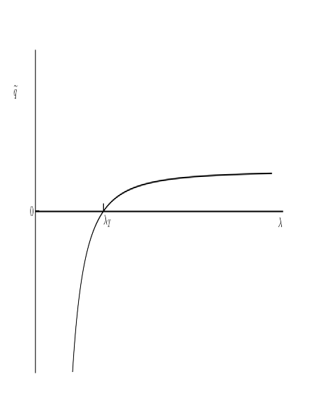
Figure 2: The linear profile of the deceleration parameter ($\tilde{q}$) measured by observers at the centre of a locally contracting bulk flow in a tilted almost-Bianchi universe with realistic anisotropy and pressureless dust. The transition scale ($\lambda_{T}$) marks the threshold where the sign of $\tilde{q}$ appears to change from positive to negative. On scales much larger than the transition length, the locally measured deceleration parameter approaches the CMB value (i.e. $\tilde{q}\rightarrow q$). Note that we have assumed subhorizon-sized bulk flows with $\vartheta=\langle\vartheta\rangle=$ constant throughout their interior. Introducing scale-dependence to $\vartheta$ does not change the key features of the $\tilde{q}$-profile, but allows to estimate the transition redshift and the current value of $\tilde{q}$ (e.g. see Fig. 3 in [30] for details).

4.4 The Bianchi transition length

Going back to expression (19), consider a contracting bulk flow (with $\vartheta<0$) in a perturbed tilted Bianchi universe with non-negligible anisotropy (i.e. set $|\zeta|/H\lesssim 1$). In this more general case, it is possible to make the local deceleration parameter negative, by appealing to both the anisotropy ratio ($\zeta/H$) and to the scale ratio ($\lambda_{H}/\lambda$). Then, the transition scale, which marks the $\tilde{q}=0$ threshold and the apparent change from deceleration to acceleration, is given by

$$\lambda_{T}={1\over 3}\sqrt{{|\vartheta|\over[q+(2\zeta\vartheta/3H^{2})]H}}\,\lambda_{H}\,.$$ (24)

As in the sub-Hubble case (ii) discuss before, the deceleration parameter turns negative on lengths smaller that $\lambda_{T}$. Also, as expected, in the absence of any anisotropy, that is when $\zeta=0$, the above reduces to its counterpart obtained in tilted Einstein-de Sitter and generalised FRW universes (see [18, 19] and also expression (22) here). There, as well as here, the transition length is a fraction of the Hubble scale and closely analogous to the Jeans length [18]. Here, the anisotropy of the Bianchi background will increase $\lambda_{T}$ when $\zeta>0$, or decrease it if $\zeta<0$, though the effect is weak in either case (in realistically anisotropic models with $|\zeta|/H\ll 1$).

According to the current observations, the anisotropy of the universe is small (if any). Therefore, in all realistic scenarios we may assume that $|\zeta|/H\ll 1$. Then, on sub-horizon scales, expressions (19) and (24) are replaced by their tilted Einstein-de Sitter counterparts, namely by Eqs. (21) and (22) respectively. Applying these relations to the observational data, one can estimate the associated values of the deceleration parameter and of the corresponding transition scale measured by observers living inside the reported bulk peculiar flows (see Table 2).

Table 2: Representative estimates of the deceleration parameter ($\tilde{q}$ – see Eq. (21)), as measured by observers residing in some of the bulk flows reported in [6]-[11], assuming that the latter are slightly contracting. The last column provides the transition lengths ($\lambda_{T}$ – see Eq. (22)), marking the $\tilde{q}=0$ threshold. Note that the scale dependence seen in (21), according to which the peculiar-motion effect on $\tilde{q}$ increases on smaller scales and decreases as we move on to larger lengths, is clearly manifested in this Table. Also, the transition length exceeds the bulk-flow scale in all cases. Finally, we have set $q=1/2$, $\vartheta=\langle\vartheta\rangle\simeq\langle v\rangle/\lambda$ and $H\simeq 70$ km/sec Mpc today.

	Survey	$\lambda~{}({\rm Mpc})$	$\langle v\rangle~{}({\rm km/s})$	$\tilde{q}$	$\lambda_{T}~{}({\rm Mpc})$
	$\begin{array}[]{c}{\rm Nusser\,\&\,Davis\;(2011)}\\ {\rm Ma,\,et\,al\;(2011)}\\ {\rm Colin,\,et\,al\;(2011)}\\ {\rm Watkins,\,et\,al\;(2023)}\\ {\rm Watkins,\,et\,al\;(2023)}\end{array}$	$\begin{array}[]{c}150\\ 150\\ 250\\ 200\\ 250\end{array}$	$\begin{array}[]{c}250\\ 340\\ 260\\ 395\\ 430\end{array}$	$\begin{array}[]{c}-2.66\\ -3.92\\ -0.24\\ -1.72\\ -0.69\end{array}$	$\begin{array}[]{c}375\\ 430\\ 300\\ 415\\ 375\end{array}$

5 Discussion

Imagine a passenger sitting in the back of a car that drives in a wide motorway, with all the cars moving at the same speed. Suppose also that, without the passenger realising it, their car slows down a little. Everyday experience then tells us that this can easily mislead the unsuspecting passenger to believe that it is the rest of the vehicles that have accelerated away. Is it then possible that something analogous can also happen to observers residing in a slightly contacting bulk peculiar flow? Is it possible that the unsuspecting observers may misinterpret their slower local expansion rate as recent global acceleration of the surrounding universe?

The theoretical possibility that the accelerated expansion of the universe is a mere illusion triggered by our peculiar motion was originally raised in [18, 19]. That scenario was later revisited and refined, by applying relativistic perturbation theory to a tilted Einstein-de Sitter model [17, 18] and subsequently extended to include all three FRW universes [19]. The latter study found that neither the pressure nor the spatial curvature could significantly change the relative-motion effects on the local deceleration parameter. The only exception was in the case of Friedmann universes with closed spatial sections, but with unrealistically high positive curvature [19]. In all these studies, observer’s living inside bulk peculiar flows, like those reported in [4]-[11] for example, could be easily misled to believe that their universe was accelerating. This could happen if the bulk flows in question were locally contracting, which is what our local peculiar-velocity field may be actually doing [29]. Then, the unsuspecting observers could misinterpret their local contraction as acceleration of the surrounding universe, just like passengers in a car that slows down may think that the vehicles around them have accelerated away.

Here we have extended the work of [18, 19] to anisotropic Bianchi-type universes. Our aim was to investigate whether the effects of anisotropy could significantly change the tilted Einstein-de Sitter picture. We found that, in principle, the shear anisotropy of the Bianchi spacetimes could modify the relative-motion effects on the locally measured deceleration parameter, either by enhancing or by reducing them. Nevertheless, unless the universe has unrealistically high anisotropy, the results of the Einstein-de Sitter scenario reported in [17, 18] remain unchanged. This is especially true on subhorizon scales, where the crucial scale-dependence (${\lambda_{H}/\lambda}$) of the peculiar-motion effects reported in [17]-[19] is identical to the one seen in Eq. (19) here. Put another way, as with the pressure and the spatial curvature, the anisotropy does not seem capable of altering the Einstein-de Sitter picture. Slightly contracting bulk peculiar motions, like those recently reported in [29], can create the illusion of global acceleration by causing an apparent change in the sign of the local deceleration parameter (see Table 2 above). The effect is local, but the transition length, where the deceleration parameter appears to turn negative, is large enough (of the order of few to several hundred Mpc) to look like a recent global event [17]-[19]. Overall, for all practical purposes, the relative-motion effects on the locally measured deceleration parameter are generic and persist irrespective of the equation of state of the matter, of the amount of spatial curvature and of the anisotropy of the background spacetime. This raises the intriguing possibility that the scale-dependent effects discussed here and in [17]-[19] within the limits of the linear analysis, may even dominate the nonlinear phase of structure formation, since on the associated scales the ratio ${\lambda_{H}/\lambda}$ can take considerably larger values.

The tilted-universe scenario does not appeal to exotic matter or/and to new physics to address the ongoing question of the universal acceleration. There is neither dark energy nor a cosmological constant, and the scenario operates within standard general relativity and conventional cosmology. Instead, the recent accelerated expansion of the universe is explained as a local illusion triggered by the peculiar motion of our galaxy. The latter is an inevitable byproduct of the structure-formation process and a hard observational fact, all of which provide a solid physical motivation to the tilted scenario. Moreover, since peculiar motions were only recently added to the kinematics of our universe, the tilted model faces no “coincidence problem” either.

In addition to its simplicity and physical motivation, the proposed scenario also makes four specific predictions that can be tested against the observations. The first is the predicted profile of the deceleration parameter, which takes positive values on sufficiently high redshifts and naturally turns negative nearby (see Fig. 2 in § 4.3 above). The second is the trademark signature of relative motion, namely an apparent (Doppler-like) dipole in the observed distribution of the deceleration parameter, like the one reported in [31]. In other words, as measured in the reference frame of the bulk-flow observers, the universe should appear to accelerate faster along one direction in the sky and equally slower in the opposite [19]. Most crucially, given that peculiar velocities fade away on progressively larger scales, the magnitude of the $q$-dipole should decrease with redshift as well.

Acknowledgements: We wish to thank Kerkyra Asvesta for her help with Fig. 2. CGT also acknowledges financial support from the Hellenic Foundation for Research and Innovation (H.F.R.I.), under the “First Call for H.F.R.I. Research Projects to support Faculty members and Researchers and the procurement of high-cost research equipment Grant” (Project No. 789).

References

- [1] A. Kogut, et al., Astrophys. J. 419, 1 (1993).
- [2] P.A.R. Ade et al., Astron. Astrophys. 561, A97 (2014).
- [3] A. Kashlinsky, F. Atrio-Barandela, D. Kocevski, H. Ebeling, Astrophys. J. 686, L49 (2009).
- [4] R. Watkins, H.A. Feldman and M.J. Hudson, Mon. Not. R. Astron. Soc. 392, 743 (2009).
- [5] G. Lavaux, R.B. Tully, R. Mohayaee, S. Colombi, Astrophys. J. 709, 483 (2010).
- [6] J. Colin, R. Mohayaee, S. Sarkar, A. Shafieloo, Mon. Not. R. Astron. Soc. 414, 264 (2011).
- [7] Y.-Z. Ma, C. Gordon and H.A. Feldman, Phys. Rev. D 83, 103002 (2011).
- [8] A. Nusser and M. Davis, Astrophys. J. 736, 93 (2011).
- [9] M.I. Scrimgeour, et al., Mon. Not. R. Astron. Soc. 455, 386 (2016).
- [10] A. Salehi, M. Yarahmadi, S. Fathi and K. Bamba, Mon. Not. R. Astron. Soc. 504, 1304 (2021).
- [11] R. Watkins, et al, Mon. Not. R. Astron. Soc. 524, 1885 (2023).
- [12] C.G. Tsagas, A. Challinor and R. Maartens, Phys. Rep. 465, 61 (2008).
- [13] G.F.R. Ellis, R. Maartens and M.A.H. MacCallum, Relativisyic Cosmology (Cambridge University Press, Cambridge, 2012).
- [14] E. Tsaprazi and C.G. Tsagas, Eur. Phys. J. C 80, 757 (2020).
- [15] C.G. Tsagas, Mon. Not. R. Asron. Soc. 405, 503 (2010).
- [16] C.G. Tsagas, Phys. Rev. D 84, 063503 (2011).
- [17] C.G. Tsagas and M.I. Kadiltzoglou, Phys. Rev. D 92, 043515 (2015).
- [18] C.G. Tsagas, Eur. Phys. J. C 81, 753 (2021).
- [19] C.G. Tsagas, Eur. Phys. J. C 82, 521 (2022).
- [20] J. Wainwrite and G.F.R. Ellis, Dynamical Systems in Cosmology (Cambridge University Press, Cambridge, 1997).
- [21] N.J. Secrest, et al, Astrophys. J. Lett. 908, L51 (2021).
- [22] C. Krishnan, J. Mondol and M.M. Seikh-Jabbari, Eur. Phys. J. C 83, 874 (2003).
- [23] R. Maartens, Phys. Rev. D 58, 124006 (1998).
- [24] G.F.R. Ellis, H. van Elst and R. Maartens, Class. Quantum Grav. 18, 5115 (2001).
- [25] G.F.R. Ellis and C.G. Tsagas, Phys. Rev. D 66, 124015 (2002).
- [26] M. Maglara and C.G. Tsagas, Phys. Rev. D 106, 083505 (2022).
- [27] C.G. Tsagas [arXiv:2404.16719].
- [28] J.A.R. Cembranos, A.L. Maroto, H. Villarrubia-Rojo, JCAP 06, 041 (2019).
- [29] E. Pasten, S. Galvez and V.H. Cardenas, Phys. Dark Univ. 43, 101385 (2023).
- [30] K. Asvesta, L. Kazantzidis, L. Perivolaropoulos and C.G. Tsagas, Mon. Not. R. Astron. Soc. 513, 234 (2022).
- [31] J. Colin, R. Mohayaee, M. Rameez and S. Sarkar, Astron. Astrophys. 631, L13 (2019).