Material Barriers to the Diffusion of the
Magnetic Field
Abstract
Recent work has identified objective (frame-indifferent) material barriers that inhibit the transport of dynamically active vectorial quantities (such as linear momentum, angular momentum and vorticity) in Navier-Stokes flows. In magnetohydrodynamics (MHD), a similar setting arises: the magnetic field vector impacts the evolution of the velocity field through the Lorentz force and hence is a dynamically active vector field. Here, we extend the theory of active material barriers from Navier-Stokes flows to MHD flows in order to locate frame-indifferent barriers to the diffusive transport of the magnetic field in turbulent two-dimensional and three-dimensional MHD flows. From this approach we obtain an algorithm for the automated extraction of such barriers from MHD turbulence data.
keywords:
Magnetohydrodynamics, Magnetic diffusion, Coherent Structures1 Introduction
The motion of Lagrangian fluid particles in magnetohydrodynamic (MHD) flows is inherently tied to the topology of the magnetic field lines, i.e., smooth curves tangent to the magnetic field, through the Lorentz force. In an ideal medium with no magnetic diffusion, magnetic field lines evolve as regular material curves: they are advected by the fluid velocity as if they were frozen to the MHD flow. Contrarily, in the presence of magnetic diffusion (finite resistivity), strong gradients in the magnetic field typically give rise to experimentally observable current filaments or sheets, i.e., thin regions with high current density (Low & Wolfson, 1988; Schrijver et al., 2001; Galsgaard et al., 2004; Zhdankin et al., 2013; Santos-Lima et al., 2021). Induced by the diffusion of the magnetic vector field, these sheets have far-reaching consequences on the transport of fluid particles as well as on the topology of magnetic field lines (Biskamp, 1986; Cowley et al., 1997; Carbone et al., 1990; Wilmot-Smith et al., 2005). Understanding the fundamental processes involved in the magnetic diffusion is crucial in describing MHD flows. Moreover, spatial structures arising in intermittent turbulence influence the dissipation, heating, transport and acceleration of charged particles (Matthaeus et al., 2015) both in laboratory and astrophysical plasmas.
Existing coherent structure diagnostics in MHD flows rely on individual snapshots of the velocity and magnetic fields (Portela et al., 2007; Zhdankin et al., 2013; Rempel et al., 2013; De Giorgio et al., 2017; Yang et al., 2017; Greco et al., 2008). Such an Eulerian description, however, fails to highlight important transport barriers that are active over a longer time interval. So far, a Lagrangian analysis in MHD flows has purely been limited to computing advective Lagrangian Coherent Structures (LCSs) (Falessi et al., 2015; Rempel et al., 2017; Chian et al., 2019; Rempel et al., 2023). These govern primarily the transport and mixing of Lagrangian fluid particles (Haller, 2023). In ideal MHD flows (with zero viscosity and resistivity ), magnetic field lines evolve as material vectors and hence are indeed tied to advective LCSs. However, in MHD flows with non-zero magnetic diffusion, magnetic field lines no longer evolve as regular material vectors, i.e., their tangent vectors do not satisfy the equations of variations
| (1) |
where is a material vector attached to the trajectory generated by the velocity field . Advective LCSs, therefore, are generally insufficient for describing the diffusive transport of magnetic field lines. Furthermore, LCS detection tools have frequently been employed to visualize invariant manifolds of the instantaneous magnetic field (Borgogno et al., 2011; Rempel et al., 2013; Rubino et al., 2015). Transport barriers obtained in this fashion are, however, not material in unsteady flows.
Here we seek active barriers to the diffusive transport of the magnetic field that have an observable impact on the fluid.
These barriers are, therefore, physical features that are intrinsic to the MHD fluid. As such, they need to be indifferent to the choice of the frame of reference (Lugt, 1979), so that two observers that are related to each other via non-relativistic, Euclidian frame changes of the type
| (2) |
identify the exact same material barriers. Here is a time-dependent translation and is a time-dependent rotation matrix. Objectivity is, therefore, a minimal self-consistency requirement for experimentally reproducible coherent structure diagnostics both in MHD and Navier-Stokes flows.
The present work builds upon the recent theory developed in Haller et al. (2020b) which seeks frame-indifferent (objective) material barriers to the transport of active vectorial quantities in 2D and 3D Navier-Stokes flows. Examples of such active vector fields in fluids include the vorticity and the linear momentum. Specifically, barriers to the diffusive transport of linear momentum, give rise to observable coherent structures in wall-bounded turbulence (Aksamit & Haller, 2022) and Rayleigh-Bénard flows (Aksamit et al., 2023).
For MHD flows, the magnetic field qualifies as a dynamically active vector since it contributes to the linear momentum equation through the Lorentz force. In our work, we seek frame-indifferent material barriers to the diffusive transport of magnetic field. These objective transport barriers are special material surfaces across which the diffusive magnetic flux vanishes pointwise.
The outline of this paper is as follows. In section 2, we first introduce our set-up and notation. We then discuss advective transport barriers and review relevant aspects of LCSs. Subsequently, we derive Eulerian and Lagrangian barriers to the diffusive transport of the magnetic field. In section 3, we compute such active magnetic field barriers for forced 2D and 3D homogenous isotropic turbulence data as streamcurves of a particular vector field. We offer a systematic comparison between magnetic barriers, linear momentum barriers and advective LCSs in MHD flows. Finally, we compute active barriers to the diffusive transport of the magnetic field and linear momentum in the solar atmosphere using the Bifrost numerical simulation tool (Gudiksen et al., 2011).
2 Methods
We consider a 3D electrically conducting fluid with velocity field and magnetic field known at spatial locations in a bounded invariant set at times . In the non-relativistic (low-frequency) regime, the forced MHD fluid satisfies the set of visco-resistive MHD equations (Davidson, 2002; Griffiths, 2005; Eringen & Maugin, 2012)
| (3) | ||||
| (4) | ||||
| (5) |
where is the total pressure field, is the Lorentz force, is an external force, and and respectively denote the kinematic viscosity and the magnetic diffusivity of the fluid. The diffusive term originates from Ohm’s constitutive material law
| (6) |
where is the electric field and
| (7) |
is the electric current density vector. The Lorentz force
| (8) | ||||
| (9) |
couples the magnetic field to the equations of motion of the fluid particle. The magnetic field vector appears on the right hand side of the linear momentum equation (3) and actively controls the dynamics of the velocity field. Here we use typical Alfvén units (Aluie, 2009).
Lagrangian particle trajectories generated by the velocity field are solutions of the differential equation
| (10) |
We denote the time- position of a trajectory starting from at time by
| (11) |
where is the flow map induced by . A material surface is a time dependent codimension-one manifold transported by the flow map from its initial position as
| (12) |
The material surface is uniquely determined by its unit normal vector at each point at time .
2.1 Advective Barriers
Advective barriers are passive material surfaces, whose evolution does not directly change the dynamics of the velocity field. Defining material barriers to advective transport is challenging because all material surfaces perfectly inhibit the transport of passive tracers. In contrast, LCSs are distinguished material surfaces that act as centerpieces to the material deformation and thereby maintain coherence over a sustained time interval (see Haller (2015)). Hyperbolic LCSs are locally the most repelling or attracting codimension-one material surfaces over a finite time interval. Attracting and repelling LCSs mimic unstable and stable invariant manifolds in autonomous dynamical systems. Elliptic LCSs are closed and nested shear-maximizing material surfaces analogous to KAM-tori. Repelling, attracting and elliptic LCSs converge to classic stable, unstable and elliptic (KAM-tori) invariant manifolds if such manifolds exist in the infinite time limit (Haller, 2015, 2023).
The right Cauchy-Green strain tensor associated with the flow map is defined as (Truesdell & Noll, 2004)
| (13) |
This symmetric and positive definite tensor encodes the Lagrangian deformation in the fluid over the finite time interval at . To visualize hyperbolic LCSs from trajectories generated from a 3D vector field over a finite time window , we define the finite time Lyapunov exponent
| (14) |
where is the largest eigenvalue of . The field is an objective Lagrangian diagnostic that measures locally the largest material stretching rate in the flow. Ridges of the field obtained from a forward trajectory integration () mark initial positions of repelling LCSs (generalized stable manifolds) at time . Similarly, ridges of the backwards field () denote initial positions of attracting LCSs (generalized unstable manifolds) at time .
In order to detect elliptic LCSs, we employ the Lagrangian-averaged vorticity deviation (LAVD), by Haller et al. (2016) defined over the finite time interval as
| (15) |
where denotes the vorticity and the overhat indicates spatial averaging over a fixed flow domain . The LAVD depends on the choice of the domain over which the spatial averaging is performed. Once is fixed, the LAVD is objective, i.e. frame-invariant with respect to frame changes of the type (2). For our computations, the domain is set to be the full computational domain as also done in Aksamit et al. (2023). In 2D, elliptic LCSs at time correspond to the outermost convex level sets of the field surrounding a unique local maximum. This definition can also be extended to 3D flows, where elliptic LCSs are identified as toroidal iso-surfaces of the field surrounding a codimension-two ridge (Neamtu-Halic et al., 2019).
2.2 Active Magnetic Barriers
The magnetic flux through a control surface is commonly defined as the surface integral of the normal component of the magnetic field over that surface (Davidson, 2002; Griffiths, 2005; Ryutova et al., 2015)
| (16) |
where is the normal vector to the surface . Following formula (16), measures the net number of magnetic field lines passing through a control surface at some fixed time . The definition of magnetic flux given in formula (16), however, suffers from several limitations for the purposes of defining an objective intrinsic diffusive flux through a co-moving material surface over the time-interval . First of all, every closed material surface results in zero net flux across the control surface due to Gauss’s law
| (17) |
Secondly, formula (16) only captures the instantaneous transport of magnetic field lines through a fixed control surface. It fails to quantify the overall diffusive transport of the magnetic field through a co-moving material surface .
Finally, the flux of a quantity through a surface should have the units of that quantity divided by time and multiplied by the surface area. This is not the case for the existing magnetic flux definition from formula (16), because has the units of times the surface area.
To resolve these ambiguities, we define the diffusive transport of the magnetic vector through a material surface over the time-interval following the approach by Haller et al. (2020b). Specifically, the transport equation for the magnetic field vector (4) can be decomposed into a diffusive and non-diffusive component
| (18) |
with and . Magnetic field lines are transported either via diffusion () or advection (). In the absence of magnetic diffusion, the magnetic field lines are advected by the velocity field as regular material lines.
We now define the instantaneous (Eulerian) diffusive transport of the magnetic field through a material surface as
| (19) | ||||
Physically, measures the extent to which the diffusive component of the rate of change of the magnetic field vector along trajectories is transverse to . As expected, the functional has no explicit dependence on the velocity field. Note that fluid trajectories do not even need to physically cross the surface to induce a diffusive magnetic field transport. The diffusive flux has the physical units expected for the flux of the magnetic vector: It is given by the units of the magnetic field multiplied by area and divided by time.
In order to obtain the diffusive Lagrangian magnetic flux, we integrate the Eulerian flux along trajectories defining the evolving material surface , which yields
| (20) | ||||
Under non-relativistic Euclidian frame changes of the form (2), the magnetic field vector is a frame-indifferent vector field, because it transforms as an objective vector (Müller et al., 2023)
| (21) |
Since the rotation matrix has no spatial dependence, it remains unaffected by spatial differentiation and the Laplacian of is also guaranteed to transform properly . Under an observer change of the form (2), the transformation formula
for the unit normal vector implies that both the Eulerian and the Lagrangian diffusive transport of the magnetic field vector are objective because
| (22) |
and similarly
| (23) |
Thanks to its inherent frame-indifference, the Eulerian and Lagrangian active magnetic barriers can be thought of as intrinsic physical properties of the surface and flow. Indeed, they are specifically tied to the fluid and do not depend on the reference frame of the observer.
Using the surface-element deformation formula (Gurtin et al., 2010)
| (24) |
we can parametrize the functional over its initial material surface as
| (25) |
with
| (26) |
Later positions of can be obtained through material advection (see relationship (12)). To keep our notation simple, we denote the temporal average of a Lagrangian vector field as
| (27) |
We also introduce as the pullback operator of an Eulerian vector field under the flow map to the initial configuration at
| (28) |
Using the notation (27-28), we obtain the simplified expression
| (29) |
and we rewrite formula (25) as
| (30) |
We seek active Lagrangian barriers to the magnetic vector field as material surfaces along which the integrand in the transport functional vanishes pointwise. This occurs if is everywhere tangent to . These material surfaces necessarily coincide with streamsurfaces (i.e., codimension-one invariant manifolds) of the autonomous vector field . We parametrize the streamlines of with , i.e., they satisfy the differential equation
| (31) |
where we have denoted differentiation with respect to by a prime. By taking the limit in formula (20), we obtain the diffusive Eulerian magnetic flux
| (32) |
Therefore, material surfaces minimizing coincide with streamsurfaces of
| (33) |
This leads us to formulating the following definition:
Definition 1
For electrically conducting fluid flows, exact Eulerian and Lagrangian barriers to the diffusive (resistive) transport of the magnetic field are structurally stable invariant manifolds of
| (34) | ||||
| (35) |
The barrier fields (34)-(35) define a 3D, autonomous (or steady) dynamical system. The structural stability guarantees that the barriers are robust with respect to small volume-preserving perturbations in the underlying vector field (Guckenheimer & Holmes, 2013). The barrier fields remain valid also for spatially and temporally dependent magnetic diffusivity as long as . We can always parametrize the trajectories generated by the barrier field (34) with respect to the rescaled barrier time
| (36) |
An analogous statement also holds for the trajectories satisfying the active Lagrangian barrier field (35). This implies that the topology of the barrier fields (34-35) is not affected by temporally and spatially dependent magnetic diffusivity.
Even the Lagrangian barrier field (35) is a steady vector field once we fix the initial and final time. All the relevant information about the time evolution of and over the time interval is encoded in the pullback and the temporal averaging operations. The instantaneous version (34) only contains the physical time as a single parameter. The Eulerian barrier field is always a divergence free vector field because is divergence free due to Gauss’s law for magnetism. This holds even for compressible fluids. In contrast, in compressible flows, the Lagrangian barrier field (35) is generally not divergence free.
By construction, all of the trajectories of the barrier fields (34)-(35) are exact barriers to the Eulerian (or Lagrangian) diffusive magnetic flux. Certain transport barriers, however, stand out because of their unique topology (e.g. they are closed and convex), while others because of their strength. To obtain a direct measure of the local strength of an active barrier, we introduce the geometric flux density
| (37) |
as defined by MacKay (1994). Here, is a general active barrier field. For example, when treating instantaneous active magnetic barriers, we set . Along an exact active barrier to the transport of , the geometric flux density vanishes pointwise. In analogy with the Diffusion Barrier Strength () defined in Haller et al. (2018, 2020a), the local strength of an active barrier field is given by the Active Barrier Strength
| (38) |
This follows from the fact that the geometric flux density will change the most under a small change in the relative position of the vectors and at locations where is the largest. As a result, the provides an objective and robust scalar diagnostic field that highlights the most influential active transport barriers. Analogous to ridges of the field that highlight the most influential diffusive transport minimizers in the flow, we can detect exceptionally strong active barriers as codimension-one ridges of the field (Haller et al., 2018, 2020a).
Note, however, that ridges of the field only serve as approximate barriers to the transport of . In 2D, we can exactly compute the most influential active barriers as streamlines of passing through local maxima of the field. Since we expect the most influential barriers to be characterized by high values, we launch trajectories from local maxima of the and stop the trajectory integration once the falls below a predefined threshold . The identified barriers are robust because local maxima and ridges of a scalar field are topologically robust features (Karrasch & Haller, 2013), i.e., they persist with respect to small volume-preserving perturbations to the underlying field. Additionally, to filter out small scale barriers linked to noise, we discard trajectory segments shorter than . For the same reason, we only retain trajectory segments whose minimal distance to nearby barriers exceeds . The exact computational details are provided in the Algorithm 1.
Input: 2D active barrier field over a regular meshgrid .
Output: Strongest active barriers blocking the transport of .
| (39) |
In 3D flows, 2D invariant manifolds of can only be determined approximately. To obtain active transport barriers that inhibit large fluxes of , we first evaluate the field over a cross-section of the selected domain. Each individual ridge of the field corresponds to a smooth curve that forms a set of initial conditions for which we compute streamlines of . Analogously to the 2D case, we only retain trajectory segments whose pointwise is greater than . For each ridge, we obtain a distinguished active transport barrier by fitting a surface through the set of streamlines. These barriers act as 2D surfaces that locally divide the domain into two regions that exchange minimal amounts of .
Input: 3D active barrier field over a regular meshgrid .
Output: Strongest active barriers blocking the transport of .
| (40) |
2.2.1 Two-Dimensional Incompressible MHD fluids
In volume-preserving (incompressible) MHD fluids we have
| (41) |
We can therefore rewrite the Lagrangian barrier equation (35) as
| (42) |
In 2D incompressible MHD flows, we can derive analytical expressions for the barrier equations from Definition 1. The visco-resistive MHD equations (3-4) then reduce to a pair of advection-diffusion equations
| (43) | ||||
| (44) |
where is the magnetic scalar potential. The vorticity and the electric current density are both scalars and given by
and
The streamfunction and the scalar magnetic potential then act as time-dependent Hamiltonians to the velocity and magnetic field
| (45) | ||||
| (46) |
with and the incompressibility of the magnetic field implies
| (47) |
With this notation, we obtain the following results on active magnetic barriers in incompressible 2D MHD flows.
Theorem 1
For incompressible, electrically conducting 2D fluid flows, exact Eulerian and Lagrangian barriers to the diffusive (resistive) transport of magnetic field are structurally stable invariant manifolds of
| (48) | ||||
| (49) |
where denotes the temporal average over the time-interval of the electric current density along a fluid trajectory .
2.3 Active Linear Momentum Barriers
Active barriers to the diffusive transport of linear momentum in Navier-Stokes flows arise due to viscous/diffusive forces in the flow (Haller et al., 2020b). Here is the constant density of the fluid and is universally set to . We can obtain momentum barriers for MHD flows by following the same principles. Specifically, as in our treatment of the active magnetic barriers, we decompose the right hand side of the linear momentum equation in MHD flows (3) into diffusive (viscous) and non-diffusive (non-viscous) components. Here, the only diffusive force in the MHD momentum equation (3) is given by and we obtain for 3D MHD flows the exact same momentum barrier fields as for 3D Navier-Stokes flows:
| (50) | ||||
| (51) |
In 2D MHD flows the linear momentum barrier fields are Hamiltonian and simplify to
| (52) | ||||
| (53) |
where denotes the temporal average over the time-interval of the vorticity along a fluid trajectory . Note that for the momentum barriers, the vorticity plays the same role as the electric current density in the active magnetic barrier equations (48)-(49). For a detailed derivation of the 2D and 3D linear momentum barriers we refer to the original work by Haller et al. (2020b).
3 Results
We now illustrate the numerical implementation of our results on high resolution 2D and 3D MHD turbulence simulations. The codes are available in the GitHub repository https://github.com/EncinasBartos together with snapshots of the datasets.
3.1 Two-dimensional MHD Turbulence
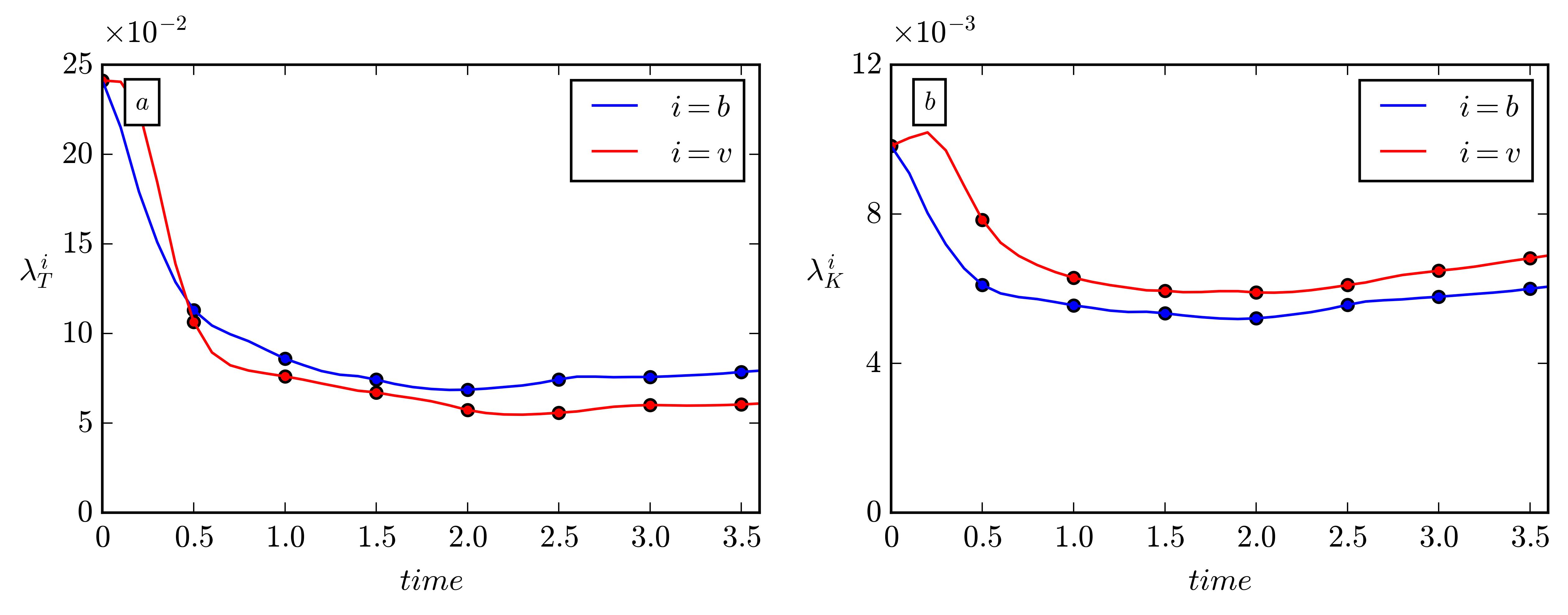
The velocity field and the magnetic scalar potential are obtained by solving the set of 2D incompressible MHD equations (43)-(44) on a periodic domain (De Giorgio et al., 2017; Servidio et al., 2010). We compute the nonlinear terms using a pseudo-spectral technique, applying a 2/3 dealiasing rule. Time integration is achieved through a classical second order Runge-Kutta method with a meshgrid resolution of points. The spatial gradients are obtained through spectral differentiation. As customary, to simulate homogeneous turbulence, we impose large-scale initial conditions, populating the lowest Fourier modes, and using random phases. As a post-processing step, we apply a Gaussian filter with standard deviation to the velocity field and the electric current density field. The kinematic viscosity and the magnetic diffusivity are both set to . The numerical simulation spans a temporal domain of and we record snapshots every . In total we have 37 snapshots that resolve the 2D MHD turbulence simulation at high fidelity. Figure 1, shows the Kolmogorov and Taylor length scales of the magnetic and velocity field as a function of time. At time , the numerical simulation reaches a statistically stationary state.
In the following, we compare active magnetic, momentum and advective transport barriers at different times of the 2D MHD turbulence simulation. We first compute Eulerian barriers at time and then extract Lagrangian barriers over time-interval and .
3.1.1 Eulerian barriers
For the instantaneous magnetic and momentum barrier calculations, we use snapshots of the vorticity and electric current density field at fully developed turbulence at time (see Fig. 2). In 2D incompressible MHD flows, both the magnetic and momentum barrier fields are Hamiltonian. Every level set of the electric current density (panel b) is an exact barrier to the diffusive flux of the magnetic field. Similarly, level sets of the vorticity (panel e) qualify as perfect barriers to the diffusive momentum transport. Out of the infinitely many candidate curves, we seek the most influential momentum and magnetic barriers over the domain (see Fig. 2). We systematically extract these barriers by following the procedure outlined in Algorithm 1. For this purpose, we first compute the field associated to the instantaneous magnetic and momentum barrier fields (see panels a,d). We then launch streamlines of the corresponding barrier field from local maxima (circles in panels b,e) of the field to obtain exact active transport barriers. Here, we set to be equal to the spatial average of the in the selected domain. Additionally, the minimum barrier length is set to and the minimal distance between two influential active barriers is . For momentum barriers (white curves in Fig. 1) we use the kinematic length scales (), whereas for the magnetic barriers (black curves in Fig. 1) we use magnetic length scales ().
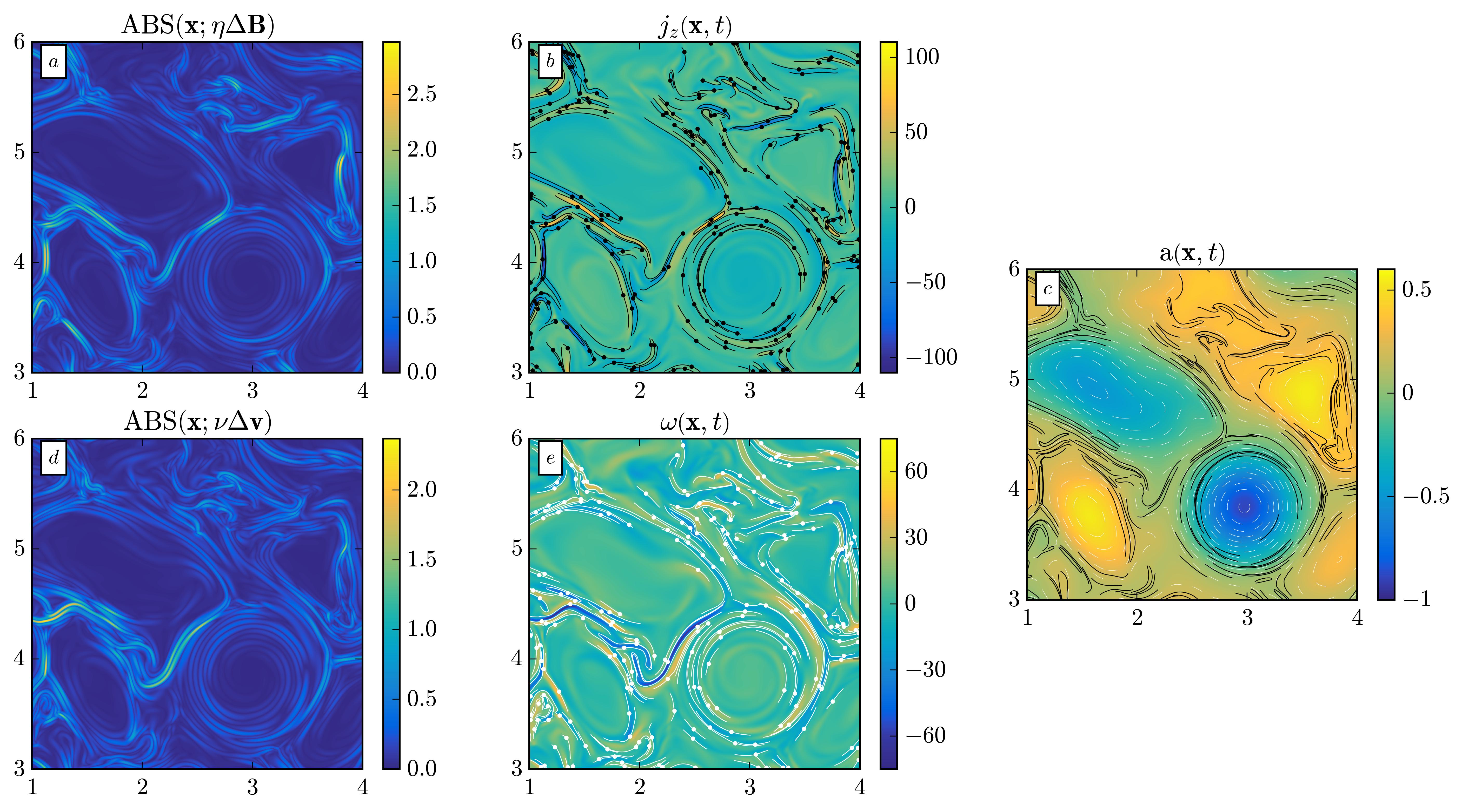
In panel (c), we have included a snapshot of the magnetic potential , which is a frequently used coherent structure diagnostic in MHD flows (Servidio et al., 2010, 2011). Level sets of correspond to magnetic field lines and are highlighted as white dashed contours. The scalar magnetic potential shows multiple elliptic islands that are surrounded by a complex pattern of active magnetic barriers. Specifically, these barriers separate elongated strips of intense electric current density, that are visible as ridges and trenches of (Cowley et al., 1997; Donato et al., 2013; Zhdankin et al., 2013). These elongated peaks and troughs in the electric current density field manifest as electric current sheets, which play an important role in magnetic reconnection—a process where magnetic energy is converted to the kinetic and thermal energy of the particles (Biskamp, 1986, 1994). We observe a similar pattern in the vorticity field, where vorticity filaments are separated by momentum barriers (see white curves in Fig. 2).
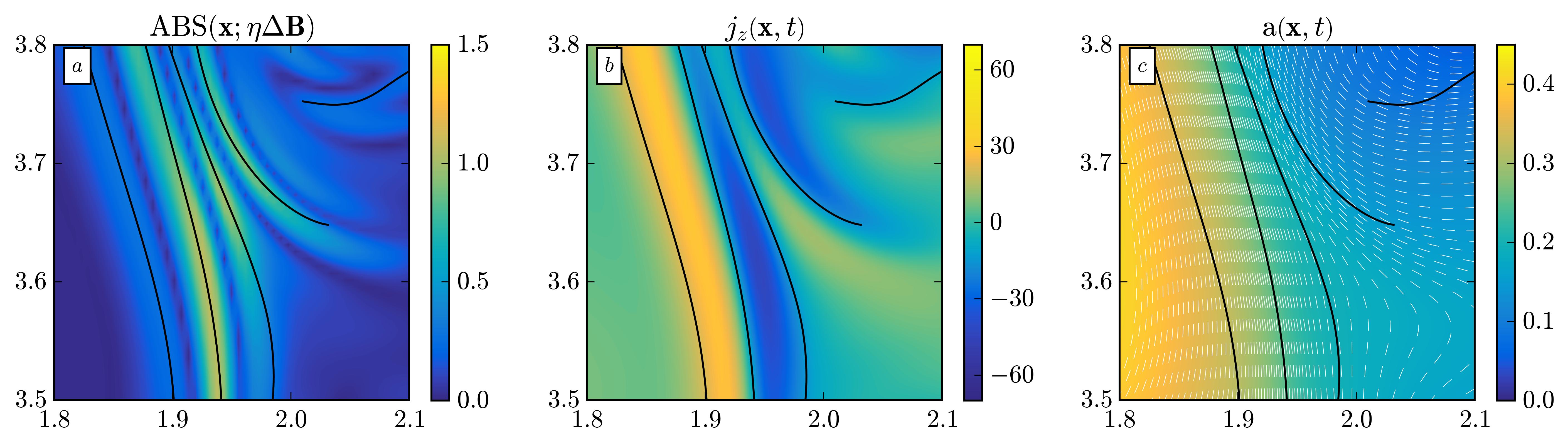
Figure 3 focuses on adjacent electric current sheets in the region . We first emphasize that the active barriers closely align with ridges of the underlying field, as already suggested in section 2.2. The principal electric current sheets are clearly visible as trenches and ridges of which are surrounded by a set of active magnetic barriers (black curves). Active magnetic barriers provide a clear demarcation of electric current sheets, suggesting no diffusive transport of the magnetic field between adjacent current sheets. Instead, dissipation of the magnetic field is constrained to occur along the active magnetic barriers, as these barriers are defined as curves tangential to the diffusive term in the magnetic transport equation (4). Despite providing critical information about underlying magnetic coherent structures, active magnetic barriers remain generally hidden in magnetic potential plots.
3.1.2 Lagrangian barriers
For the Lagrangian barrier calculations, we first compute the Lagrangian averages and along fluid trajectories using all the available snapshots between and over the domain . Based on that, we compute expressions for the active barrier fields from (49) and (53). To visualize advective LCSs at time , we plot the and fields over the initial conditions . We recall that ridges of the field mark initial positions of the most repelling material lines (repelling LCS), whereas convex level sets of surrounding an isolated local maximum indicate rotationally coherent structures (elliptic LCS).
Figure 4 shows the field computed for the Lagrangian magnetic and momentum barrier fields from (49-53) (see panels a, b). We then extract exact active material barriers by following the procedure outlined in Algorithm 1. For the active Lagrangian magnetic barrier calculations we set and , whereas for the momentum barriers we use the corresponding kinematic length scales. Here, the black curves mark active magnetic material barriers, whereas the white curves indicate momentum blocking material barriers. Similarly to the case of the Eulerian barriers, ridges of the field closely align with exact active transport barriers in our Lagrangian computations (see Fig. 4). Active magnetic barriers (black curves in Fig. 4) mark sharp edges in the Lagrangian-averaged electric current density field , thereby separating the domain into areas with minimal time-averaged magnetic diffusion. Likewise, momentum barriers occur at sharp edges of the Lagrangian-averaged vorticity field . Note that, the Hamiltonians and resemble features found in the and fields. This is to be expected because level sets of Lagrangian-averaged scalar fields occasionally relate to advective LCSs, that are obtained from purely kinematic computations (Kelley et al., 2013; Hadjighasem et al., 2017).
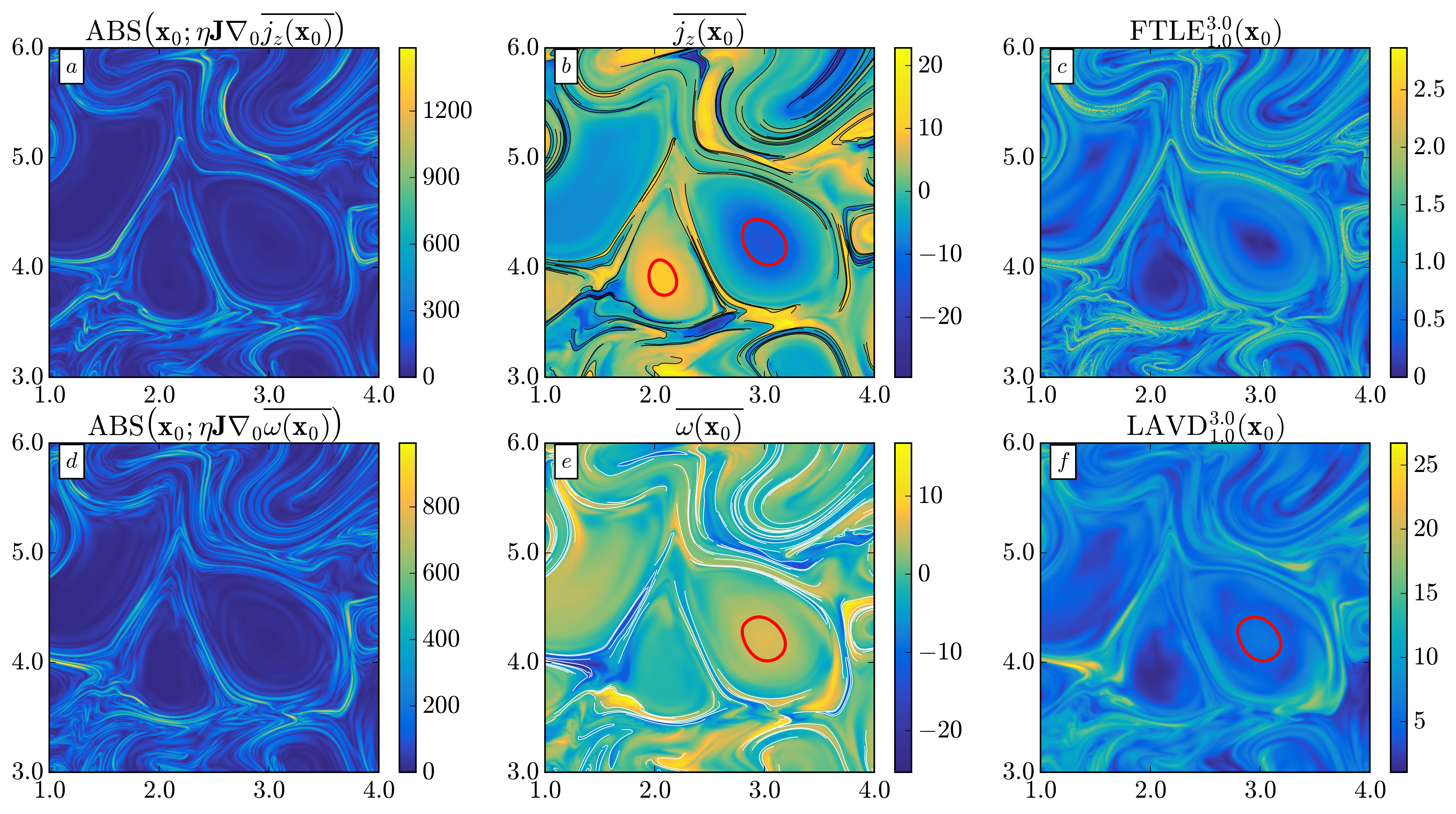
Next, we compute LAVD-based vortex boundaries as outermost closed and convex level sets surrounding a unique local maximum of (Haller et al., 2016). We only retain large-scale vortices whose perimeter is greater than . In 2D incompressible MHD flows the Lagrangian active barrier fields are Hamiltonian, governed by the appropriate Hamiltonian function . Therefore, we can extract elliptic active barriers as outermost convex level sets of surrounding a unique local maximum of (Haller et al., 2020b). For active Lagrangian magnetic barriers we set , whereas for the momentum barriers we set .
The elliptic barriers computed from the underlying scalar field are shown as red curves in Fig. 4. The momentum and -based vortices are practically indistinguishable, whereas shows the existence of a magnetic vortex pair (see panel b).
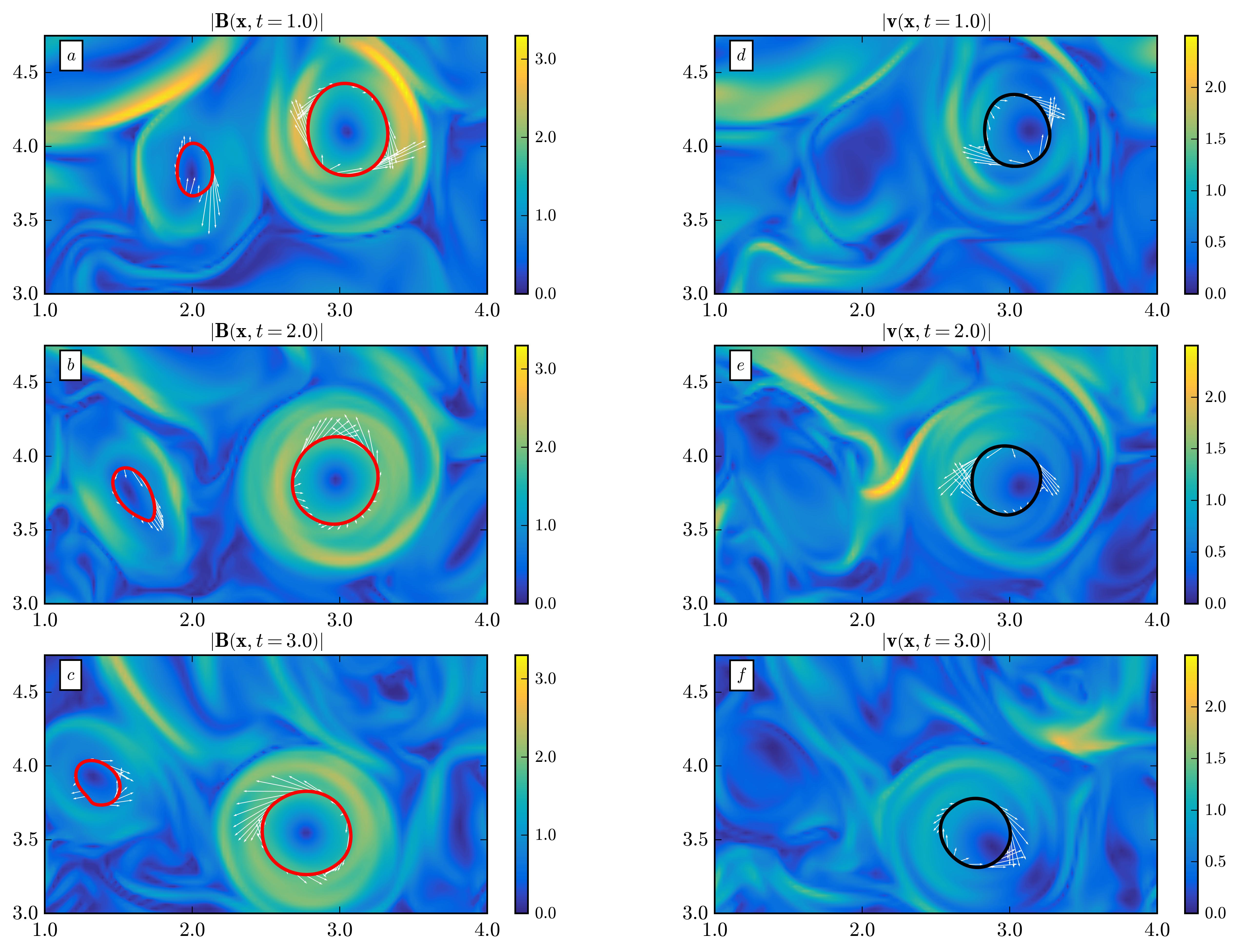
We now examine the temporal evolution of the magnetic vortex pair (depicted by red curves in the left column of Fig. 5) and illustrate its impact on the magnetic field within the time span . Additionally, we overlay the advected momentum-based vortex (represented by the black curve in the right column of Fig. 5) on top of the normalized linear momentum field. Notably, we observe that both active barriers exhibit no signs of filamentation throughout the entire duration. This is consistent with our earlier expectation for elliptic coherent structures. Furthermore, the active magnetic barriers keep enclosing regions of low magnetic field intensity throughout the extraction period. Similarly, active barriers consistently encapsulate small values of the linear momentum norm.
Figure 5 also shows the instantaneous active barrier fields along the respective active magnetic and momentum barriers. Note that the extracted barriers closely align with the underlying instantaneous active barrier fields for most of the time. Nonetheless, there are some notable exceptions, indicating that these barriers do not exactly minimize the instantaneous diffusive transport of the magnetic field or momentum at every time instance. Instead, active material barriers minimize the underlying diffusive transport of the magnetic field or momentum in a time-averaged sense.
In the Supplementary Material we have added a simulation of the active material barriers in Fig. 5 over the complete time-interval .
3.2 Three-dimensional MHD Turbulence
In the following, we use forced MHD turbulence data from the Johns Hopkins Turbulence Database (JHTDB) (Perlman et al., 2007; Li et al., 2008; Aluie, 2009; Eyink et al., 2013). The data was generated by a direct numerical simulation of the 3D incompressible MHD equations, in a cubic domain of size with periodic boundary conditions and resolution . The kinematic viscosity and magnetic diffusivity are both equal to and the kinematic and magnetic Kolmogorov length scales are respectively and . The flow is forced at large scales in the plane by a steady Taylor-Green body force
| (54) |
with .
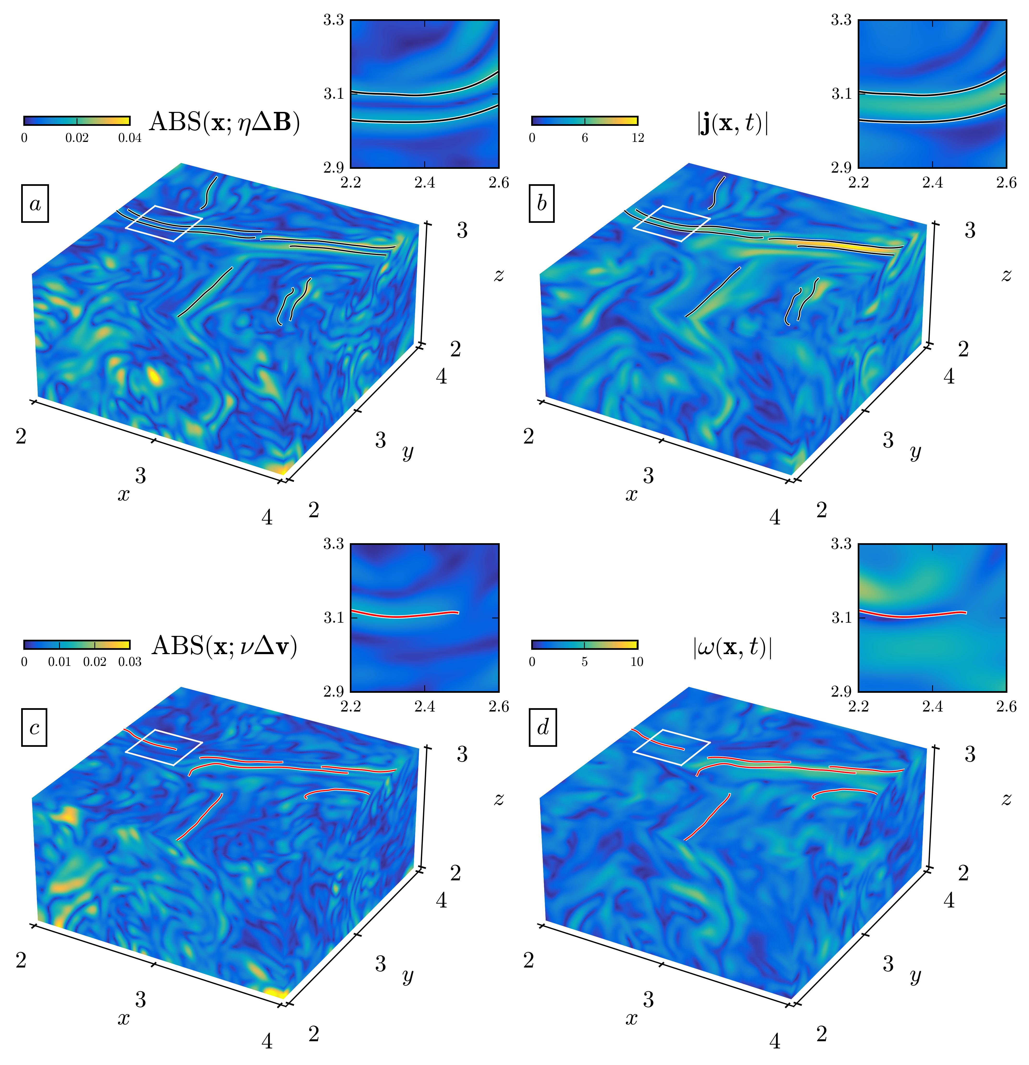
In Fig. 6 we compare the field for the magnetic (panel a) and momentum (panel c) barrier fields with the electric current density (panel b) and the normed vorticity (panel d) over the domain . The zoomed inset in Fig. 6a shows two prominent ridges (black curves) of the that delineate the boundary of an electric current sheet (see zoomed inset in panel b). Similarly, ridges of the (red curves) wrap around vorticity filaments also in 3D (see zoomed inset in panel d).
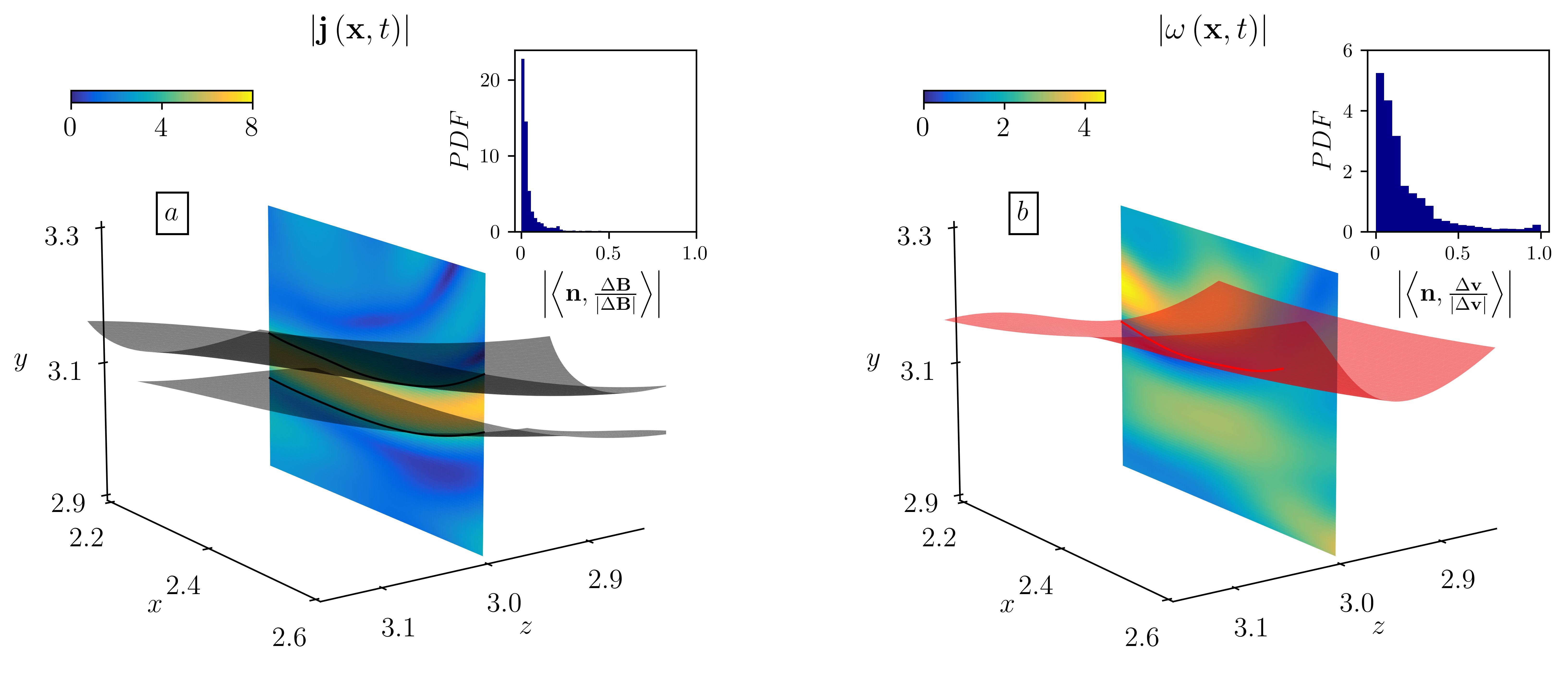
Next, we focus on the region in the plane which is shown in the zoomed inset of Fig. 6 and extract instantaneous active magnetic and momentum barriers using the Algorithm 2. We approximate Eulerian active magnetic barriers, by fitting polynomial surfaces of degree to streamlines of (34) launched from ridges (black curves) of . Here, we set to be equal to the spatial average of in the selected domain and the maximum arclength of the streamline is chosen to be . For the momentum blocking barriers we follow a similar reasoning and replace the magnetic with the momentum quantities. Figure 7a displays two active magnetic barriers (black surfaces) that trace out the boundary of an electric current sheet. Similarly, the red surface in Fig. 7b corresponds to an approximate momentum-barrier separating two vorticity filaments.
To test the transport blocking ability of the identified surface with respect to the underlying barrier field, we compute the pointwise normalized flux by taking the inner product between the normal vector of the surface and the corresponding normalized active barrier field. If the surfaces computed according to Algorithm 2 were exact streamcurves of the barrier equation, then their normals would be pointwise perpendicular to the underlying barrier field. The inset in panel (a) displays the probability distribution of the normed inner product between and the unit vector of over both active magnetic barriers. Similarly, the inset of panel (b) shows the probability distribution of the pointwise tangency between the active momentum barrier field and the corresponding momentum blocking surface (red). Both distributions show a prominent peak at . This suggests that barriers obtained according to Algorithm 2 are close approximations to perfect active barriers.
3.3 Bifrost-Stellar Atmosphere Simulation
Finally, we identify active magnetic barriers in the solar atmosphere using the numerical dataset obtained from the Bifrost code (Gudiksen et al., 2011; Carlsson et al., 2016). When numerically solving the MHD equations, the diffusive operator is split in a global diffusive term and a local hyper diffusion term in order to maintain numerical stability. The splitting of the diffusive terms into local and global components makes it possible to run the code at higher Reynolds numbers. Hence, in principle, the magnetic diffusivity and the kinematic viscosity vary in space and time, whereby these fluctuations are assumed to be small on average. We stress that the local fluctuations of the diffusive terms are purely a numerical procedure to guarantee stability. For more details we refer to the work done by Gudiksen et al. (2011); Carlsson et al. (2016); Færder et al. (2023).
The computational domain spans horizontally across a area with periodic boundary conditions. Vertically, it extends 2.4 below the visible surface, and 14.4 above, encompassing the upper layers of the convection zone, photosphere, chromosphere, and solar corona. With a grid size of points, the computational resolution is 48 horizontally, while vertically, the grid separation varies from 19 in the photosphere and chromosphere and then gradually increases to 100 at the upper boundary. We select the snapshot at of the en024048_hion simulation which is publicly available from the European Hinode Science Data Centre (http://www.sdc.uio.no/search/simulations). This simulation snapshot has already been used in prior works by Leenaarts et al. (2013a, b); de la Cruz Rodriguez et al. (2013).
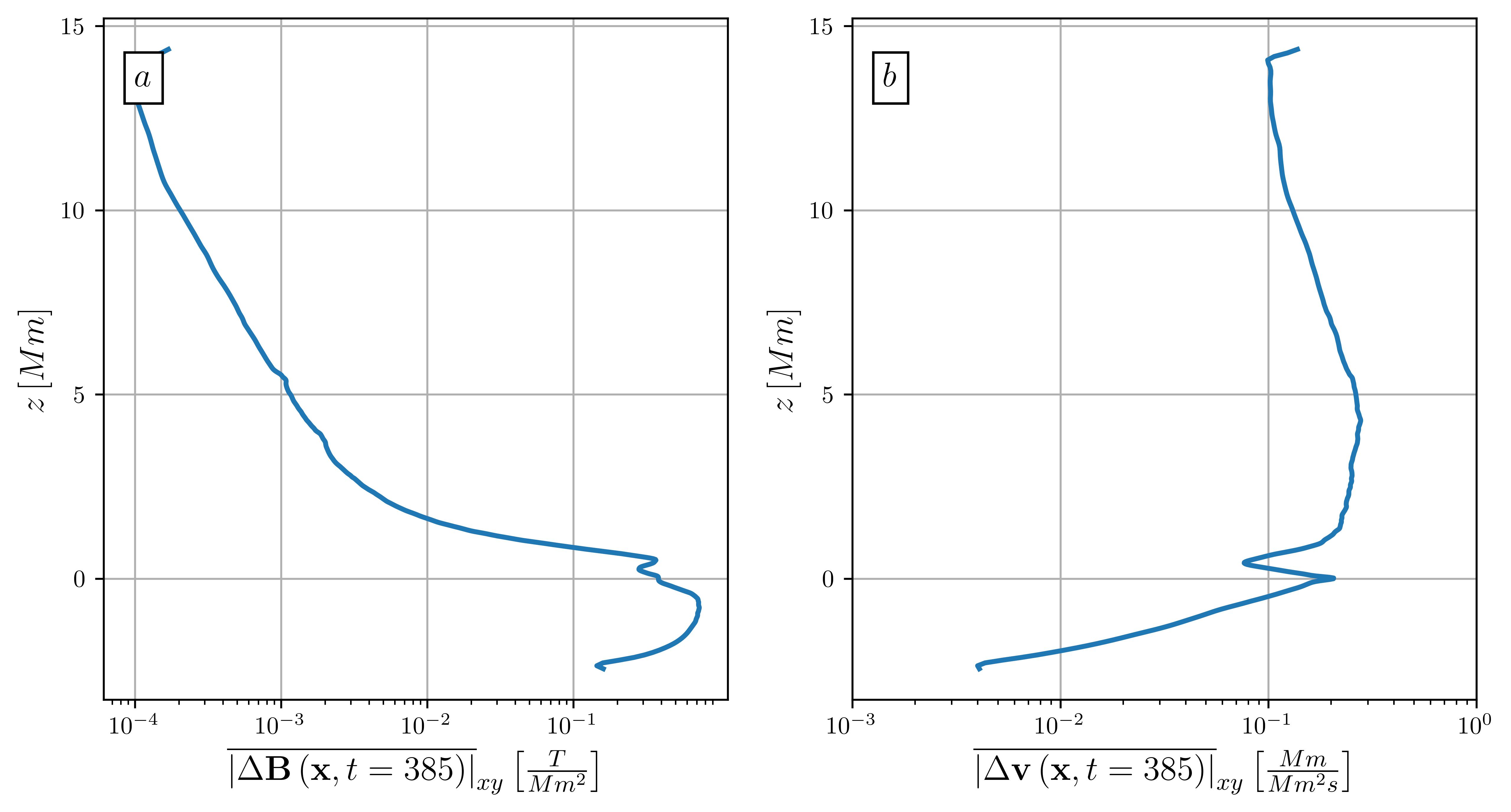
The solar atmosphere exhibits various layers of stratification in the vertical direction, each characterized by distinct properties and characteristic length scales. Within these layers, the Laplacian of the velocity and the magnetic fields undergo notable variations as shown in Fig. 8, where we have computed the spatial average over the plane of and as a function of the vertical direction. Given a scalar field , we use the notation to indicate spatial averaging over the domain. Both and vary substantially over multiple scales in the -direction. To allow for a scale-independent visualization of the transport barriers in the solar atmosphere over different layers, we normalize all scalar fields in the direction with their corresponding spatial average in the plane. Here, we use the subscript to denote the normalized scalar field. Note that the geometry of the magnetic and momentum barriers remains unaffected by this normalization.
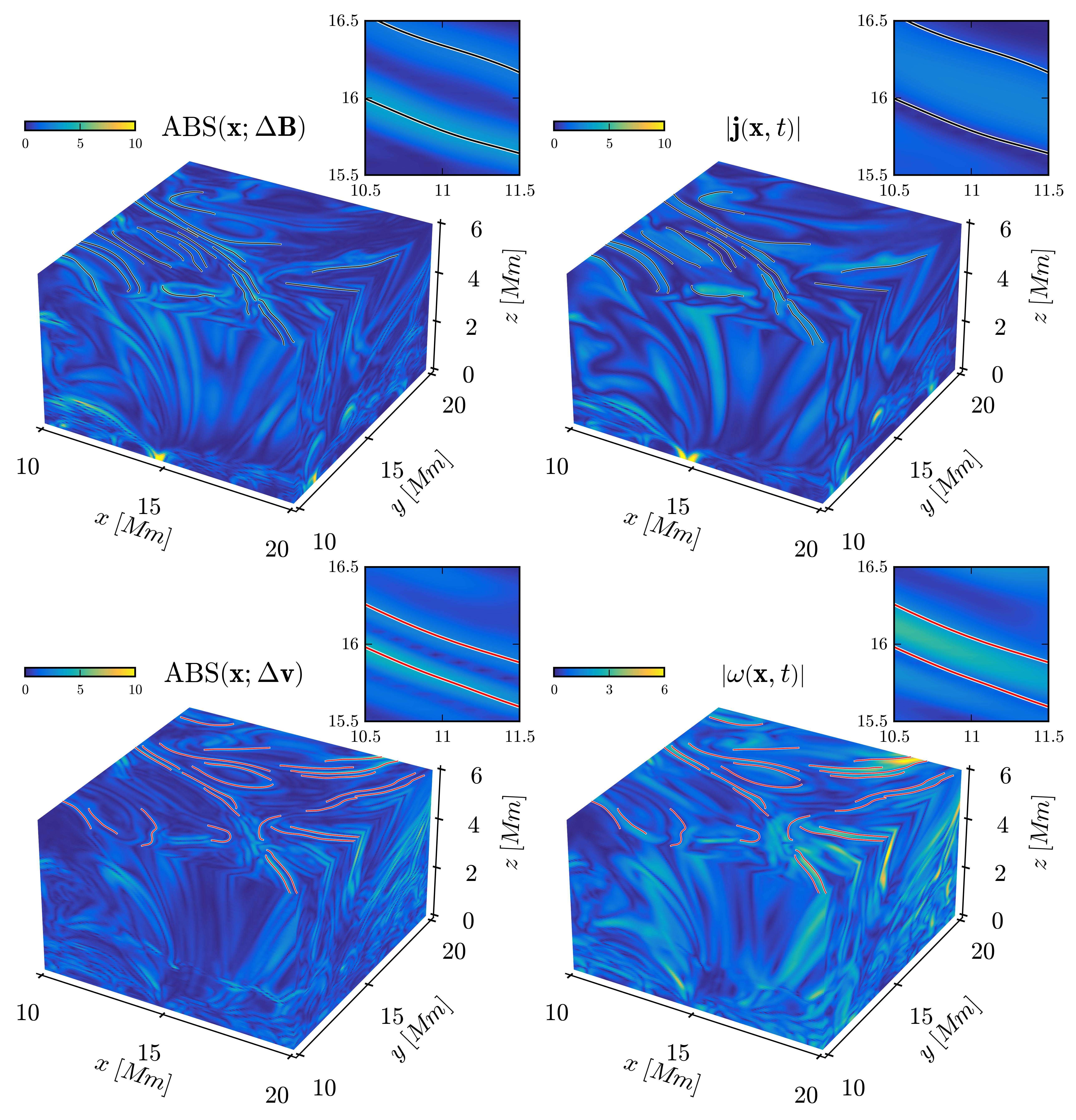
In Fig. 9, we calculate the normalized field across a cubic domain for both the instantaneous magnetic (panel a) and momentum (panel c) barrier fields. Additionally, snapshots of the normalized electric current density (panel b) and vorticity (panel d) are provided. Ridges of the magnetic and momentum-based fields form smooth curves that mark the intersection of the most influential active transport barriers with the plane. To approximate parametric surfaces that inhibit the diffusive transport of the magnetic field or linear momentum, we follow the procedure outlined in Algorithm 2, by utilizing cubic polynomials (). Here, we set the maximum arclength of the streamlines to be equal to and equal to the spatial average of the underlying field.
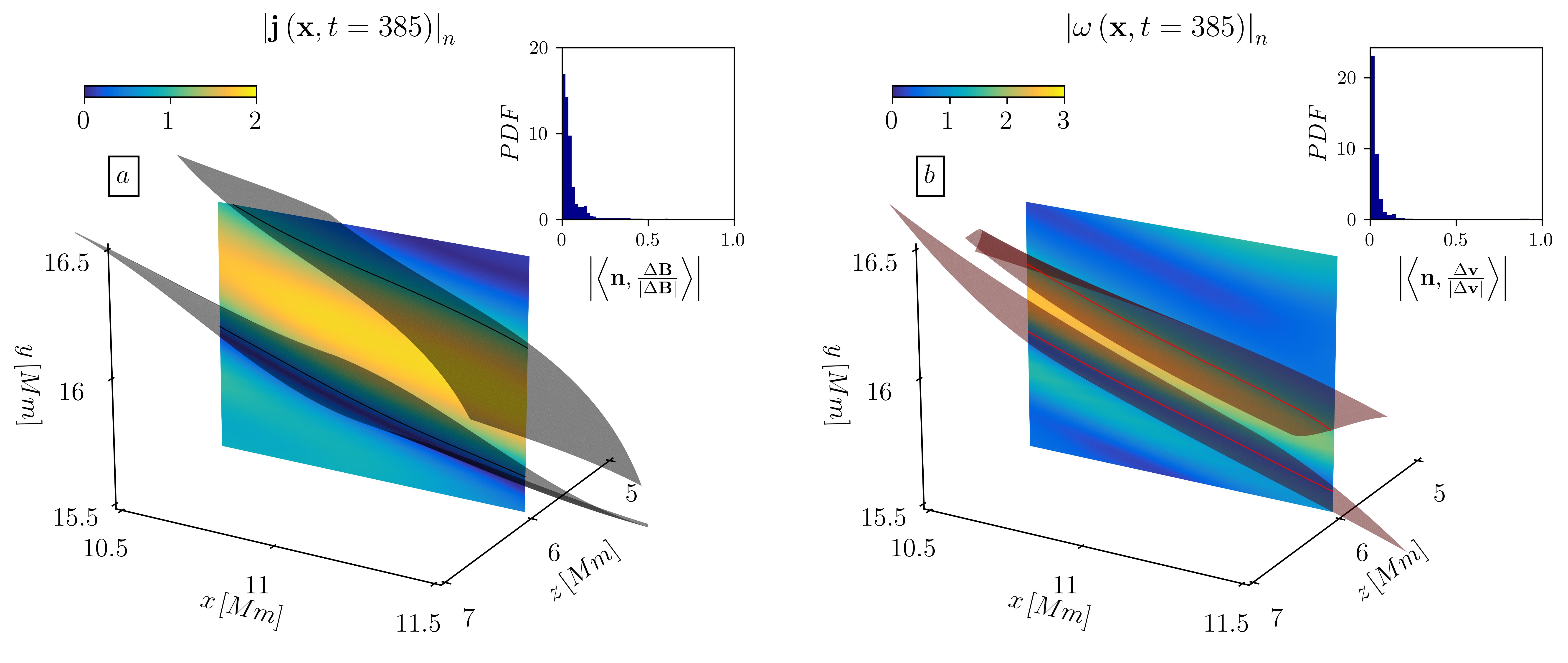
In Fig. 10, we examine the approximate active magnetic (panel a) and momentum (panel b) transport barriers within the zoomed inset area of Fig. 9. Analogous to the findings in the 3D MHD turbulence simulation outlined in section 3.2, instantaneous active magnetic transport barriers delineate the boundary of an electric current sheet (see Fig. 10a). Similarly, the most influential active momentum barriers inhibit the diffusive momentum flux across vorticity filaments. The PDFs in the insets of Fig. 10 confirm that the computed barriers are nearly tangent to the underlying barrier fields.
4 Conclusion
Appropriately modifying the recent active barrier theory of Haller et al. (2020b) for Navier-Stokes flows, we have identified coherent structure boundaries as material surfaces that minimize the diffusive transport of the magnetic field in 2D and 3D MHD turbulence. These distinguished active magnetic barriers, locally partition the domain into two regions with minimal diffusion of the magnetic field. We have also compared active magnetic barriers with linear momentum barriers and advective LCSs. Our analysis shows that active magnetic barriers provide objective barriers to diffusive transport of the magnetic field. We have also devised an algorithm to extract the most influential active magnetic barriers in both 2D and 3D MHD flows.
In 2D incompressible MHD, active magnetic barriers can directly be obtained as level curves of appropriate Hamiltonians that are obtained from the electric current density. This stems from the fact that the equations governing these barriers form autonomous, planar Hamiltonian systems. Of the infinitely many barrier candidates, we have computed the most influential barriers as streamlines launched from local maxima of the field (see Algorithm 1).
A physical take-away message from our 2D MHD turbulence example is that the strongest Eulerian active magnetic barriers separate electric current sheets and hence induce zero diffusive transport of magnetic field across them. Instead, the dissipative transport of the magnetic field occurs along the active magnetic transport barriers we have identified. Secondly, we have computed active magnetic vortices as parametric curves from specific level sets of the Hamiltonian. As expected, the identified active magnetic vortices minimize the diffusive transport of the magnetic field and maintain coherence, i.e., they do not filament. Additionally, active Lagrangian magnetic vortices consistently encapsulate low values of the norm of the magnetic field. Overall, our numerical computations show that active magnetic barriers generally differ from advective and linear momentum barriers.
We have similarly obtained active magnetic barriers in 3D MHD turbulence over a 2D cross-section of the flow. Note, however, that in 3D the active barrier fields are no longer Hamiltonian and hence the electric current density does not directly appear in the active magnetic barrier equations. Interestingly, our numerical results on the Johns Hopkins MHD Turbulence Dataset suggest that the most influential active magnetic barriers in 3D arise at the interface between adjacent current sheets. Analogously to the case of the 2D MHD turbulence, this implies zero diffusive transport of the magnetic field across nearby current sheets.
Finally, we have tested our results also on simulations of the stellar atmosphere using the Bifrost code (Gudiksen et al., 2011). The proposed algorithm allows a scale-independent computation of active transport barriers from discrete numerical data of the magnetic and velocity field. We have verified that the computed active transport barriers closely align with exact active transport barriers by measuring the pointwise tangency between the normal of the surface and the underlying barrier field.
The objective active magnetic barriers described here are intrinsic physical features of the fluid and contribute to the understanding and identification of various turbulent flow structures in MHD flows. Future research should investigate Lagrangian magnetic, momentum and advective transport barriers in the solar atmosphere, thereby expanding on the studies from Nóbrega-Siverio et al. (2016); Leenaarts (2018). Additionally, we plan to relate the identified active magnetic barriers to dissipation of electromagnetic energy (Chian et al., 2023; Rempel et al., 2023; Silva et al., 2024; Finley et al., 2022) and thermal coherent structures (Amari et al., 2015; Cranmer & Winebarger, 2019; Loukitcheva et al., 2015) within the stellar atmosphere.
Appendix A Proof of Theorem 1
We recall that for 2D incompressible MHD flows, the magnetic field satisfies
| (55) |
with . The scalar magnetic potential satisfies the advection diffusion equation (44) and its solution along fluid trajectories is given by
| (56) |
where we have used the property and the temporal averaging operator (see formula (27)). With the notation
| (57) |
the integral form of the magnetic transport equation (4) is
| (58) |
where we used the property . By rearranging Eq.(58), we then obtain
| (59) |
Inserting formula (55) into (59) yields
| (60) |
where . Using now the chain rule for , we can write
| (61) |
where we have used the fact that in 2D incompressible flows
| (62) |
where and . By combining the relationships (60-61) we then obtain
| (63) |
Finally, combining Eq. (56) with Eqs.(63) and (59) yields
| (64) |
We then obtain the Eulerian counterpart by taking the infinitesimal limit of Eq.(64)
| (65) |
This concludes the proof.
References
- Aksamit & Haller (2022) Aksamit, N. O. & Haller, G. 2022 Objective momentum barriers in wall turbulence. Journal of Fluid Mechanics 941, A3.
- Aksamit et al. (2023) Aksamit, N. O., Hartmann, R., Lohse, D. & Haller, G. 2023 Interplay between advective, diffusive and active barriers in (rotating) rayleigh–bénard flow. Journal of Fluid Mechanics 969, A27.
- Aluie (2009) Aluie, H. 2009 Hydrodynamic and magnetohydrodynamic turbulence: invariants, cascades, and locality. The Johns Hopkins University.
- Amari et al. (2015) Amari, T., Luciani, J.-F. & Aly, J.-J. 2015 Small-scale dynamo magnetism as the driver for heating the solar atmosphere. Nature 522 (7555), 188–191.
- Biskamp (1986) Biskamp, D. 1986 Magnetic reconnection via current sheets. The Physics of fluids 29 (5), 1520–1531.
- Biskamp (1994) Biskamp, D. 1994 Magnetic reconnection. Physics Reports 237 (4), 179–247.
- Borgogno et al. (2011) Borgogno, D., Grasso, D., Pegoraro, F. & Schep, T. 2011 Barriers in the transition to global chaos in collisionless magnetic reconnection. i. ridges of the finite time lyapunov exponent field. Physics of Plasmas 18 (10).
- Carbone et al. (1990) Carbone, V., Veltri, P. & Mangeney, A. 1990 Coherent structure formation and magnetic field line reconnection in magnetohydrodynamic turbulence. Physics of Fluids A: Fluid Dynamics 2 (8), 1487–1496.
- Carlsson et al. (2016) Carlsson, M., Hansteen, V. H., Gudiksen, B. V., Leenaarts, J. & De Pontieu, B. 2016 A publicly available simulation of an enhanced network region of the sun. Astronomy & Astrophysics 585, A4.
- Chian et al. (2023) Chian, A. C., Rempel, E. L., Silva, S. S., Bellot Rubio, L. & Gošić, M. 2023 Intensification of magnetic field in merging magnetic flux tubes driven by supergranular vortical flows. Monthly Notices of the Royal Astronomical Society 518 (4), 4930–4942.
- Chian et al. (2019) Chian, A. C., Silva, S. S., Rempel, E. L., Gošić, M., Bellot Rubio, L. R., Kusano, K., Miranda, R. A. & Requerey, I. S. 2019 Supergranular turbulence in the quiet sun: Lagrangian coherent structures. Monthly Notices of the Royal Astronomical Society 488 (3), 3076–3088.
- Cowley et al. (1997) Cowley, S., Longcope, D. & Sudan, R. 1997 Current sheets in mhd turbulence. Physics reports 283 (1-4), 227–251.
- Cranmer & Winebarger (2019) Cranmer, S. R. & Winebarger, A. R. 2019 The properties of the solar corona and its connection to the solar wind. Annual Review of Astronomy and Astrophysics 57, 157–187.
- de la Cruz Rodriguez et al. (2013) de la Cruz Rodriguez, J., De Pontieu, B., Carlsson, M. & van der Voort, L. R. 2013 Heating of the magnetic chromosphere: observational constraints from ca ii 8542 spectra. The Astrophysical Journal Letters 764 (1), L11.
- Davidson (2002) Davidson, P. A. 2002 An introduction to magnetohydrodynamics.
- De Giorgio et al. (2017) De Giorgio, E., Servidio, S. & Veltri, P. 2017 Coherent structure formation through nonlinear interactions in 2d magnetohydrodynamic turbulence. Scientific Reports 7 (1), 13849.
- Donato et al. (2013) Donato, S., Greco, A., Matthaeus, W., Servidio, S. & Dmitruk, P. 2013 How to identify reconnecting current sheets in incompressible hall mhd turbulence. Journal of Geophysical Research: Space Physics 118 (7), 4033–4038.
- Eringen & Maugin (2012) Eringen, A. C. & Maugin, G. A. 2012 Electrodynamics of continua II: fluids and complex media. Springer Science & Business Media.
- Eyink et al. (2013) Eyink, G., Vishniac, E., Lalescu, C., Aluie, H., Kanov, K., Bürger, K., Burns, R., Meneveau, C. & Szalay, A. 2013 Flux-freezing breakdown in high-conductivity magnetohydrodynamic turbulence. Nature 497 (7450), 466–469.
- Færder et al. (2023) Færder, Ø. H., Nóbrega-Siverio, D. & Carlsson, M. 2023 A comparative study of resistivity models for simulations of magnetic reconnection in the solar atmosphere. Astronomy & Astrophysics 675, A97.
- Falessi et al. (2015) Falessi, M., Pegoraro, F. & Schep, T. 2015 Lagrangian coherent structures and plasma transport processes. Journal of Plasma Physics 81 (5), 495810505.
- Finley et al. (2022) Finley, A. J., Brun, A. S., Carlsson, M., Szydlarski, M., Hansteen, V. & Shoda, M. 2022 Stirring the base of the solar wind: On heat transfer and vortex formation. Astronomy & Astrophysics 665, A118.
- Galsgaard et al. (2004) Galsgaard, K., Moreno-Insertis, F., Archontis, V. & Hood, A. 2004 A three-dimensional study of reconnection, current sheets, and jets resulting from magnetic flux emergence in the sun. The Astrophysical Journal 618 (2), L153.
- Greco et al. (2008) Greco, A., Chuychai, P., Matthaeus, W., Servidio, S. & Dmitruk, P. 2008 Intermittent mhd structures and classical discontinuities. Geophysical Research Letters 35 (19).
- Griffiths (2005) Griffiths, D. J. 2005 Introduction to electrodynamics.
- Guckenheimer & Holmes (2013) Guckenheimer, J. & Holmes, P. 2013 Nonlinear oscillations, dynamical systems, and bifurcations of vector fields, , vol. 42. Springer Science & Business Media.
- Gudiksen et al. (2011) Gudiksen, B. V., Carlsson, M., Hansteen, V. H., Hayek, W., Leenaarts, J. & Martínez-Sykora, J. 2011 The stellar atmosphere simulation code bifrost-code description and validation. Astronomy & Astrophysics 531, A154.
- Gurtin et al. (2010) Gurtin, M. E., Fried, E. & Anand, L. 2010 The mechanics and thermodynamics of continua. Cambridge university press.
- Hadjighasem et al. (2017) Hadjighasem, A., Farazmand, M., Blazevski, D., Froyland, G. & Haller, G. 2017 A critical comparison of lagrangian methods for coherent structure detection. Chaos: An Interdisciplinary Journal of Nonlinear Science 27 (5).
- Haller (2015) Haller, G. 2015 Lagrangian Coherent Structures. Annu. Rev. Fluid Mech. 47, 137–162.
- Haller (2023) Haller, G. 2023 Transport Barriers in Flow Data: Advective, Diffusive, Stochastic and Active Methods. Cambridge, UK: Cambridge University Press.
- Haller et al. (2016) Haller, G., Hadjighasem, A., Farazmand, M. & Huhn, F. 2016 Defining coherent vortices objectively from the vorticity. Journal of Fluid Mechanics 795, 136–173.
- Haller et al. (2018) Haller, G., Karrasch, D. & Kogelbauer, F. 2018 Material barriers to diffusive and stochastic transport. Proceedings of the National Academy of Sciences 115 (37), 9074–9079.
- Haller et al. (2020a) Haller, G., Karrasch, D. & Kogelbauer, F. 2020a Barriers to the transport of diffusive scalars in compressible flows. SIAM Journal on Applied Dynamical Systems 19 (1), 85–123.
- Haller et al. (2020b) Haller, G., Katsanoulis, S., Holzner, M., Frohnapfel, B. & Gatti, D. 2020b Objective barriers to the transport of dynamically active vector fields. Journal of Fluid Mechanics 905.
- Karrasch & Haller (2013) Karrasch, D. & Haller, G. 2013 Do finite-size lyapunov exponents detect coherent structures? Chaos: An Interdisciplinary Journal of Nonlinear Science 23 (4).
- Kelley et al. (2013) Kelley, D. H., Allshouse, M. R. & Ouellette, N. T. 2013 Lagrangian coherent structures separate dynamically distinct regions in fluid flows. Physical Review E 88 (1), 013017.
- Leenaarts (2018) Leenaarts, J. 2018 Tracing the evolution of radiation-mhd simulations of solar and stellar atmospheres in the lagrangian frame. Astronomy & Astrophysics 616, A136.
- Leenaarts et al. (2013a) Leenaarts, J., Pereira, T. M. D., Carlsson, M., Uitenbroek, H. & De Pontieu, B. 2013a The formation of iris diagnostics. i. a quintessential model atom of mg ii and general formation properties of the mg ii h&k lines. The Astrophysical Journal 772 (2), 89.
- Leenaarts et al. (2013b) Leenaarts, J., Pereira, T. M. D., Carlsson, M., Uitenbroek, H. & De Pontieu, B. 2013b The formation of iris diagnostics. ii. the formation of the mg ii h&k lines in the solar atmosphere. The Astrophysical Journal 772 (2), 90.
- Li et al. (2008) Li, Y., Perlman, E., Wan, M., Yang, Y., Meneveau, C., Burns, R., Chen, S., Szalay, A. & Eyink, G. 2008 A public turbulence database cluster and applications to study lagrangian evolution of velocity increments in turbulence. Journal of Turbulence (9), N31.
- Loukitcheva et al. (2015) Loukitcheva, M., Solanki, S., Carlsson, M. & White, S. 2015 Millimeter radiation from a 3d model of the solar atmosphere-i. diagnosing chromospheric thermal structure. Astronomy & Astrophysics 575, A15.
- Low & Wolfson (1988) Low, B. & Wolfson, R. 1988 Spontaneous formation of electric current sheets and the origin of solar flares. Astrophysical Journal, Part 1 (ISSN 0004-637X), vol. 324, Jan. 1, 1988, p. 574-581. 324, 574–581.
- Lugt (1979) Lugt, H. J. 1979 The dilemma of defining a vortex. In Recent developments in theoretical and experimental fluid mechanics: Compressible and incompressible flows, pp. 309–321. Springer.
- MacKay (1994) MacKay, R. S. 1994 Transport in 3d volume-preserving flows. Journal of Nonlinear Science 4, 329–354.
- Matthaeus et al. (2015) Matthaeus, W. H., Wan, M., Servidio, S., Greco, A., Osman, K. T., Oughton, S. & Dmitruk, P. 2015 Intermittency, nonlinear dynamics and dissipation in the solar wind and astrophysical plasmas. Philosophical Transactions of the Royal Society A: Mathematical, Physical and Engineering Sciences 373 (2041), 20140154.
- Müller et al. (2023) Müller, W. H., Vilchevskaya, E. N. & Eremeyev, V. A. 2023 Electrodynamics from the viewpoint of modern continuum theory—a review. ZAMM-Journal of Applied Mathematics and Mechanics/Zeitschrift für Angewandte Mathematik und Mechanik 103 (4), e202200179.
- Neamtu-Halic et al. (2019) Neamtu-Halic, M., Krug, D., Haller, G. & Holzner, M. 2019 Lagrangian coherent structures and entrainment near the turbulent/non-Turbulent interface of a gravity current. Journal of Fluid Mechanics 877, 824–843.
- Nóbrega-Siverio et al. (2016) Nóbrega-Siverio, D., Moreno-Insertis, F. & Martínez-Sykora, J. 2016 The cool surge following flux emergence in a radiation-mhd experiment. The Astrophysical Journal 822 (1), 18.
- Perlman et al. (2007) Perlman, E., Burns, R., Li, Y. & Meneveau, C. 2007 Data exploration of turbulence simulations using a database cluster. In Proceedings of the 2007 ACM/IEEE Conference on Supercomputing, pp. 1–11.
- Portela et al. (2007) Portela, J. S., Caldas, I. L., Viana, R. L. & Morrison, P. 2007 Diffusive transport through a nontwist barrier in tokamaks. International Journal of Bifurcation and Chaos 17 (05), 1589–1598.
- Rempel et al. (2013) Rempel, E. L., Chian, A. C.-L., Brandenburg, A., Muñoz, P. R. & Shadden, S. C. 2013 Coherent structures and the saturation of a nonlinear dynamo. Journal of Fluid Mechanics 729, 309–329.
- Rempel et al. (2023) Rempel, E. L., Chian, A. C.-L., de SA Silva, S., Fedun, V., Verth, G., Miranda, R. A. & Gošić, M. 2023 Lagrangian coherent structures in space plasmas. Reviews of Modern Plasma Physics 7 (1), 32.
- Rempel et al. (2017) Rempel, E. L., Chian, A.-L., Beron-Vera, F. J., Szanyi, S. & Haller, G. 2017 Objective vortex detection in an astrophysical dynamo. Monthly Notices of the Royal Astronomical Society: Letters 466 (1), L108–L112.
- Rubino et al. (2015) Rubino, G., Borgogno, D., Veranda, M., Bonfiglio, D., Cappello, S. & Grasso, D. 2015 Detection of magnetic barriers in a chaotic domain: first application of finite time lyapunov exponent method to a magnetic confinement configuration. Plasma Physics and Controlled Fusion 57 (8), 085004.
- Ryutova et al. (2015) Ryutova, M., Ryutova, M. & Evenson 2015 Physics of magnetic flux tubes, , vol. 417. Springer.
- Santos-Lima et al. (2021) Santos-Lima, R., Guerrero, G., de Gouveia Dal Pino, E. & Lazarian, A. 2021 Diffusion of large-scale magnetic fields by reconnection in mhd turbulence. Monthly Notices of the Royal Astronomical Society 503 (1), 1290–1309.
- Schrijver et al. (2001) Schrijver, C. J. & others 2001 On the formation of polar spots in sun-like stars. The Astrophysical Journal 551 (2), 1099.
- Servidio et al. (2011) Servidio, S., Dmitruk, P., Greco, A., Wan, M., Donato, S., Cassak, P., Shay, M., Carbone, V. & Matthaeus, W. 2011 Magnetic reconnection as an element of turbulence. Nonlinear Processes in Geophysics 18 (5), 675–695.
- Servidio et al. (2010) Servidio, S., Matthaeus, W., Shay, M., Dmitruk, P., Cassak, P. & Wan, M. 2010 Statistics of magnetic reconnection in two-dimensional magnetohydrodynamic turbulence. Physics of Plasmas 17 (3).
- Silva et al. (2024) Silva, S. S., Verth, G., Rempel, E. L., Ballai, I., Jafarzadeh, S. & Fedun, V. 2024 Magnetohydrodynamic poynting flux vortices in the solar atmosphere and their role in concentrating energy. The Astrophysical Journal 963 (1), 10.
- Truesdell & Noll (2004) Truesdell, C. & Noll, W. 2004 The non-linear field theories of mechanics. Springer.
- Wilmot-Smith et al. (2005) Wilmot-Smith, A., Priest, E. & Hornig, G. 2005 Magnetic diffusion and the motion of field lines. Geophysical & Astrophysical Fluid Dynamics 99 (2), 177–197.
- Yang et al. (2017) Yang, Y., Matthaeus, W. H., Shi, Y., Wan, M. & Chen, S. 2017 Compressibility effect on coherent structures, energy transfer, and scaling in magnetohydrodynamic turbulence. Physics of Fluids 29 (3).
- Zhdankin et al. (2013) Zhdankin, V., Uzdensky, D. A., Perez, J. C. & Boldyrev, S. 2013 Statistical analysis of current sheets in three-dimensional magnetohydrodynamic turbulence. The Astrophysical Journal 771 (2), 124.