Towards Understanding the Working Mechanism of Text-to-Image Diffusion Model

Abstract

Recently, the strong latent Diffusion Probabilistic Model (DPM) has been applied to high-quality Text-to-Image (T2I) generation (e.g., Stable Diffusion), by injecting the encoded target text prompt into the gradually denoised diffusion image generator. Despite the success of DPM in practice, the mechanism behind it remains to be explored. To fill this blank, we begin by examining the intermediate statuses during the gradual denoising generation process in DPM. The empirical observations indicate, the shape of image is reconstructed after the first few denoising steps, and then the image is filled with details (e.g., texture). The phenomenon is because the low-frequency signal (shape relevant) of the noisy image is not corrupted until the final stage in the forward process (initial stage of generation) of adding noise in DPM. Inspired by the observations, we proceed to explore the influence of each token in the text prompt during the two stages. After a series of experiments of T2I generations conditioned on a set of text prompts. We conclude that in the earlier generation stage, the image is mostly decided by the special token [EOS] in the text prompt, and the information in the text prompt is already conveyed in this stage. After that, the diffusion model completes the details of generated images by information from themselves. Finally, we propose to apply this observation to accelerate the process of T2I generation by properly removing text guidance, which finally accelerates the sampling up to 25%+.

1 Introduction

In real-world application, the Text-to-Image (T2I) generation has long been explored owing to its wide applications [46; 31; 32; 2; 15], whereas the Diffusion Probabilistic Model (DPM) [12; 37; 32] stands out as a promising approach, thanks to its impressive image synthesis capability. Technically, the DPM is a hierarchical denoising model, which gradually purifies noisy data from a standard Gaussian to generate an image. In the existing literature [31; 34; 28; 6], the framework of (latent) Stable Diffusion model [31] is a backbone technique in T2I generation via DPM. In this approach, the text prompt is encoded by a CLIP text encoder [30], and injected into the diffusion image decoder as a condition to generate a target image (latent encoded by VQ-GAN in [31]) that is consistent with the text prompt. Though this framework works well in practice, the working mechanism behind it, especially for the text prompt, remains to be explored. Therefore, in this paper, we systematically explore the working mechanism of stable diffusion.

Our investigation starts from the intermediate status of the denoising generation process. Through an experiment (details are in Section 4), we find that in the early stage of the denoising process, the overall shapes of generated images (latent) are already reconstructed. In contrast, the details (e.g., textures) are then filled at the end of the denoising process. To explain this, we notice that the overall shape (resp. semantic details) is decided by low-frequency (resp. high-frequency) signals [9]. We both empirically show and theoretically explain that in contrast to the high-frequency signals, the low-frequency signals of noisy data are not corrupted until the end stage of the forward noise-adding process. Therefore, its reverse denoising process firstly recovers the low-frequency signal (so that overall shape) in the initial stage, and then recovers the high-frequency part in the latter stage.

Following the phenomenons, we investigate the effect of encoded tokens in the text prompt of T2I generation during the two stages, where each token is encoded by an auto-regressive CLIP text encoder. The text prompt has a length of 76, and is enclosed by special tokens [SOS] and [EOS], at the beginning and end of the text prompt, respectively. Therefore, we categorize the tokens into three classes, i.e., [SOS], semantic tokens, and [EOS]. Notably, the special token [SOS] does not contain information, due to the auto-regressive encoding of the text prompt. Thus, our investigations into the influence of tokens will primarily focus on the semantic tokens and [EOS]. Surprisingly, we find that compared with semantic tokens, the special token [EOS] has a larger impact during generation.

Concretely, under a set of collected text prompts, we select 1000 pairs “[SOS] + Prompt $A$ ($B$) + [EOS]_A(B)” from it. Then, replace the special token [EOS]_A in the text prompt $A$ with [EOS]_B from prompt $B$ to observe the generated data under this condition. Interestingly, we find that the generated images are more likely to be aligned with text prompt $B$ (especially for the shape features) instead of $A$, so that [EOS] has a larger impact compared with semantic tokens. Besides that, we further find that the information in [EOS] is already conveyed during the early shape reconstruction stage of the denoising process. Exploring along the working stage of [EOS], we further verify and explain that the whole text prompts (including semantic ones) primarily work on the early denoising process, when the overall shapes of generated images are constructed. After that, the image details are mainly reconstructed by the images themselves. This phenomenon is explained by “first shape then details”, as the injected text prompt implicitly penalizes the generated images to be consistent with it. Therefore, the penalization quickly becomes weak, when the overall shape of image is reconstructed.

Finally, we apply our observations in one practical cases: Training-free sampling acceleration, as the text prompt works in the first stage of denoising process, we remove the textual prompt-related model propagation ($\boldsymbol{\epsilon}_{\boldsymbol{\theta}}(t,\boldsymbol{x}_{t},\mathcal{C})$ in (3)) during the details reconstruction stage, which merely change the generated images but save about 25%+ inference cost.

We summarize our contributions as follows.

1. We show, during the denoising process of the stable diffusion model, the overall shape and details of generated images are respectively reconstructed in the early and final stages of it.

2. For the working mechanism of text prompt, we empirically show the special token [EOS] dominates the influence of text prompt in the early (overall shape reconstruction) stage of denoising process, when the information from text prompt is also conveyed. Subsequently, the model works on filling the details of generated images mainly depending on themselves.

3. We apply our observation to accelerate the sampling of denoising process 25%+.

2 Related Work

Diffusion Model.

In this paper, our exploration is based on the Stable Diffusion [32], which now terms to be a standard T2I generation technique based on DPM [12; 36], and has been applied into various computer vision domains e.g., 3D [29; 33; 19] and video generation [26; 4]. In practice, the goal of T2I is generating an image that is consistent with a given text injected into the cross-attention module [42] of the image decoder. Therefore, understanding the working mechanism of stable diffusion potentially improves the existing techniques [1]. Unfortunately, to the best of our knowledge, the problem is limited explored, expected in [45; 35], where they similarly observe the low-frequency signals are firstly recovered in the denoising process. However, further explanations for this phenomenon are neglected in these works.

Influence of Tokens.

Understanding the working mechanism of encoded (by a pretrained language model) text prompt [3; 30; 43; 27] helps us understanding T2I generation [38; 16; 21]. For example, [44] finds that in LLM, the first token primarily decides the weights in the cross-attention map, which similarly appeared in the cross-modality text-image stable diffusion model as we observed. [47] explores the influence of individual tokens in counterfactual memorization. However, in the multi-modality models e.g., [30; 18; 17; 23], whereas the textual information interacted with the image in the cross-attention module as in stable diffusion, the working mechanism of tokens interacts with cross-modality data is limited explored, expected in [1]. They find in a single case that the influence of text prompts may decrease during the denoising process, while they do not proceed to study or apply this phenomenon as in this paper. Recently, [48] finds that the cross-attention map between the text prompt and generated images converges during the denoising process, which is also explained by our observations that the information conveyed during the first few denoising steps. Besides that, unlike ours, their observations are lack of theoretical explanation.

3 Preliminaries

We briefly introduce the (latent) stable diffusion model [31], which transfers a standard Gaussian noise into a target image latent that aligns with pre-given text prompts. Here, the generated data space is a low-dimensional Vector-Quantized (VQ) [7] image latent to reduce the computational cost of generation. One may get the target natural image by decoding the generated image latent. In this paper, the original data (image latent) is denoted by $\boldsymbol{x}_{0}$, and the encoded textual prompt (by CLIP text encoder [30]) is represented by $\mathcal{C}$. The noisy data

$$\small\boldsymbol{x}_{t}=\sqrt{\bar{\alpha}_{t}}\boldsymbol{x}_{0}+\sqrt{1-\bar{\alpha}_{t}}\boldsymbol{\epsilon}_{t},$$ (1)

is used as input to diffusion model $\boldsymbol{\epsilon}_{\boldsymbol{\theta}}$ trained by

$$\small\min_{\boldsymbol{\theta}}\mathbb{E}\left[\left\|\boldsymbol{\epsilon}_{\boldsymbol{\theta}}(t,\boldsymbol{x}_{t},\mathcal{C},\emptyset)-\boldsymbol{\epsilon}_{t}\right\|^{2}\right],$$ (2)

with $0\leq t\leq T$, $\boldsymbol{\epsilon}_{t}\sim\mathcal{N}(0,\boldsymbol{I})$ independent of $\boldsymbol{x}_{0}$, $\bar{\alpha}_{t}\to 0$ (resp. $\bar{\alpha}_{t}\to 1$) for $t\to 0$ (resp. $t\to T$). Here, the noise prediction model $\boldsymbol{\epsilon}_{\boldsymbol{\theta}}(t,\boldsymbol{x}_{t},\mathcal{C},\emptyset)$ is constructed by classifier-free guidance [13] with

$$\small\boldsymbol{\epsilon}_{\boldsymbol{\theta}}(t,\boldsymbol{x}_{t},\mathcal{C},\emptyset)=\boldsymbol{\epsilon}_{\boldsymbol{\theta}}(t,\boldsymbol{x}_{t},\emptyset)+w\left(\boldsymbol{\epsilon}_{\boldsymbol{\theta}}(t,\boldsymbol{x}_{t},\mathcal{C})-\boldsymbol{\epsilon}_{\boldsymbol{\theta}}(t,\boldsymbol{x}_{t},\emptyset)\right),$$ (3)

where $\boldsymbol{\epsilon}_{\boldsymbol{\theta}}(t,\boldsymbol{x}_{t},\emptyset)$ is an unconditional generative model, and the $w\geq 0$ is guidance scale. As the model is trained to predict noise $\boldsymbol{\epsilon}_{t}$ in $\boldsymbol{x}_{t}$, and $\boldsymbol{x}_{T}$ approximates a standard Gaussian, we can conduct the reverse denoising process (DDIM [36]) transfers a standard Gaussian to target image $\boldsymbol{x}_{0}$

$$\small\boldsymbol{x}_{t-1}=\sqrt{\frac{\bar{\alpha}_{t-1}}{\bar{\alpha}_{t}}}\boldsymbol{x}_{t}+\left(\sqrt{\frac{1-\bar{\alpha}_{t-1}}{\bar{\alpha}_{t-1}}}-\sqrt{\frac{1-\bar{\alpha}_{t}}{\bar{\alpha}_{t}}}\right)\boldsymbol{\epsilon}_{\boldsymbol{\theta}}(t,\boldsymbol{x}_{t},\mathcal{C},\emptyset).$$ (4)

Finally, the diffusion model (usually UNet) takes the text prompt as input to the cross-attention module in each basic block of diffusion model with output ${\rm Attention}(Q,K,V)=\mathrm{Softmax}(QK^{\top}/\sqrt{d})V$ ($d$ is dimension of image feature), where $\phi(\boldsymbol{x}_{t})$ is the feature of image, and

$$\small Q=W_{Q}\phi(\boldsymbol{x}_{t});K=W_{K}\mathcal{C};V=W_{V}\mathcal{C}.$$ (5)

4 First Overall Shape then Details

In this section, we first explore the image reconstruction process of the stable diffusion model. As noted in [1], the generated image’s overall shape is difficult to be alterted in the final stage of the denoising process. Inspired by this observation, and note that the low-frequency and high-frequency signals of image determine its overall shape and details, respectively [9]. We theoretically and empirically verify that the denoising process recovers the low and high-frequency signals in its initial and final stages, respectively, which explains the phenomenon of “first overall shape then details”.

4.1 Two Stages of Denoising Process

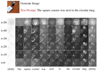
(a)

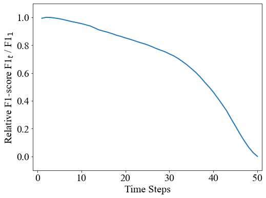
(b)

Figure 1: Figure LABEL:fig:cross-attention_map is the averaged cross-attention over denoising steps. The two generated images are on the top, and the weights in cross-attention maps of each tokens are on the bottom with whiter pixels correspond to larger weights in cross-attention map. Figure LABEL:fig:cross-attention_map_ratio is obtained by taking average over tokens and prompts in PromptSet, which compares the shapes of cross-attention map and final generated images, Measured by relative F1-score $\text{F1}_{t}/\text{F1}_{1}$ over different denoising steps.

Settings (PromptSet).

As in [14], we use 1600 prompts following the template “a {attribute} {noun}”, with the attribute as an adjective of color or texture. We create 800 text prompts respectively under each of the two categories of attributes. Besides that, we add another extra 1000 complex natural prompts in [14] without a predefined sentence template. These prompts consist of the text prompts set (abbrev PromptSet) we used. The classes of nouns, colors, and textures are respectively 230, 33, and 23 in these prompts. In this paper, we generate images under PromptSet by Stable Diffusion v1.5-Base [31]. Finally, without specification, we use 50 steps DDIM sampling [36].

From [40], though stable diffusion generates encoded VQ image latents [7]. These latents preserve semantic information transformed by text prompt through cross-attention module (5). Notably, in the cross-attention module, the pixel is a weighted sum of token embedding with cross-attention map $\mathrm{Softmax}(QK^{\top}/\sqrt{d})$ as weights. The weights reveal the semantic information of token, as they are the correlations between image query $Q$ and textual key $K$. To check the correlation, we visualize the averaged cross-attention map over all layers of model $\boldsymbol{\epsilon}_{\boldsymbol{\theta}}$ under different time steps $t$, from 50 to 1.

Interestingly, the cross-attention map of each token already has a semantic shape in the early stage of the denoising process, e.g., for $t=40$ in example Figure LABEL:fig:cross-attention_map. This can hold only if the overall shape of the image is constructed in this early stage, so that each pixel can correspond to the correct token. To further investigate this, we compute the average cross-attention map of each token under the aforementioned PromptSet. We compare the shape of the cross-attention map and the final generated image quantitatively by transforming them into canny images [9] and computing the F1-score [39] ($\text{F1}_{t}$ for each $t$) between these canny images. To compare the difference over different time steps more clearly, we plot the relative F1-score $\text{F1}_{t}/\text{F1}_{1}$ ($t=1$ the image has been recovered). The result in Figure LABEL:fig:cross-attention_map_ratio shows the shape of the cross-attention map rapidly close to the ones of the generated image in the early stage of denoising, which is consistent with our speculation and the result in [48], where they conclude that the cross-attention map will converge during the denoising process.

4.2 Frequency Analysis

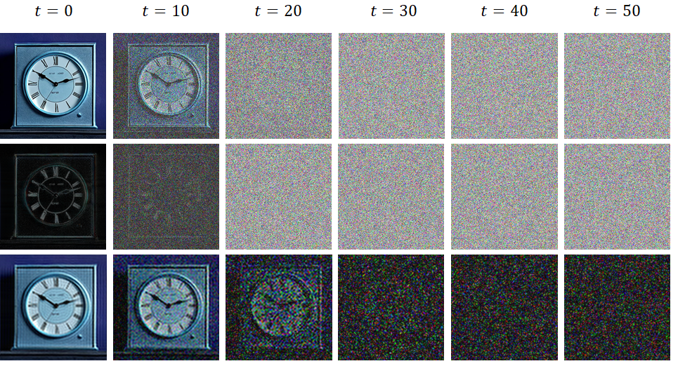
(a)

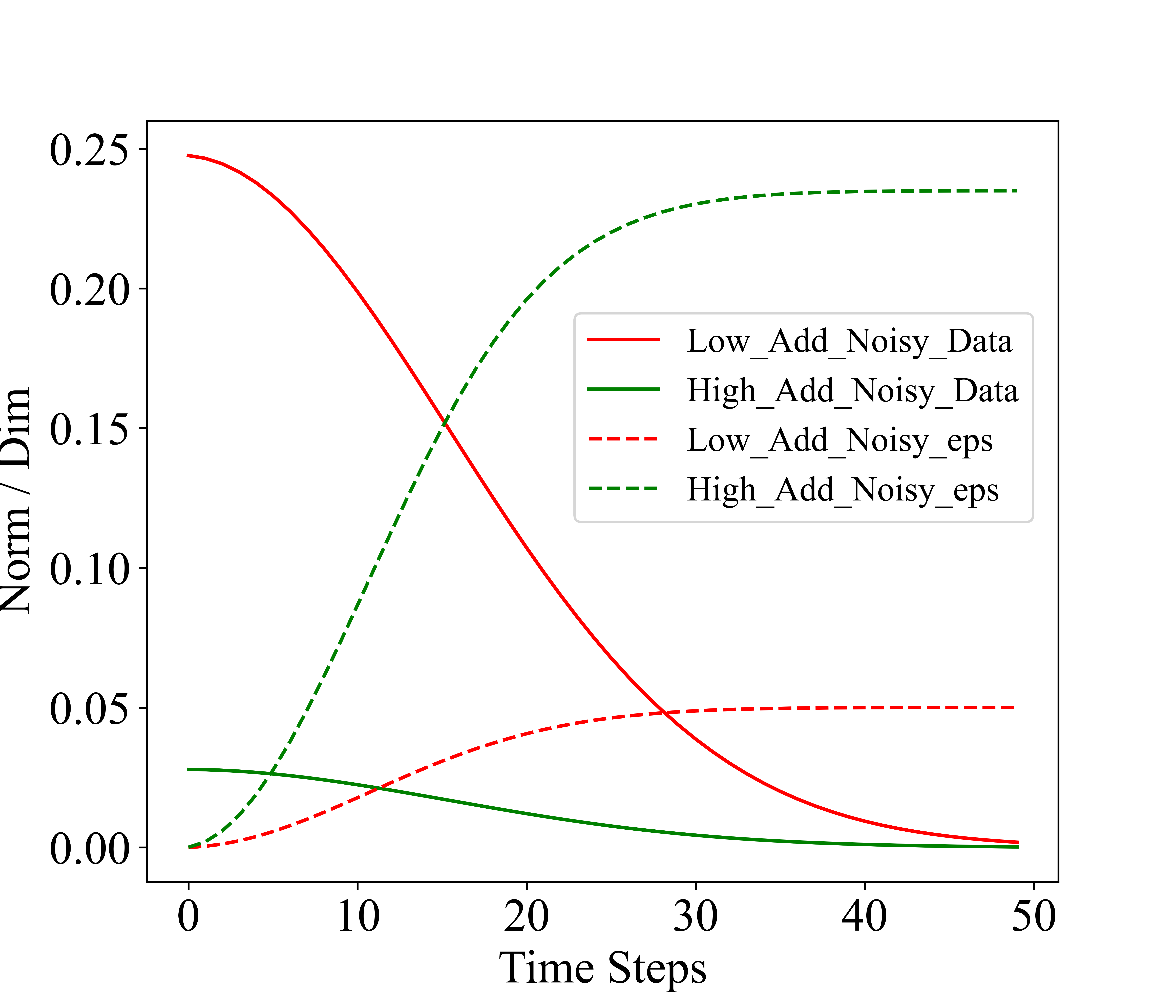
(b)

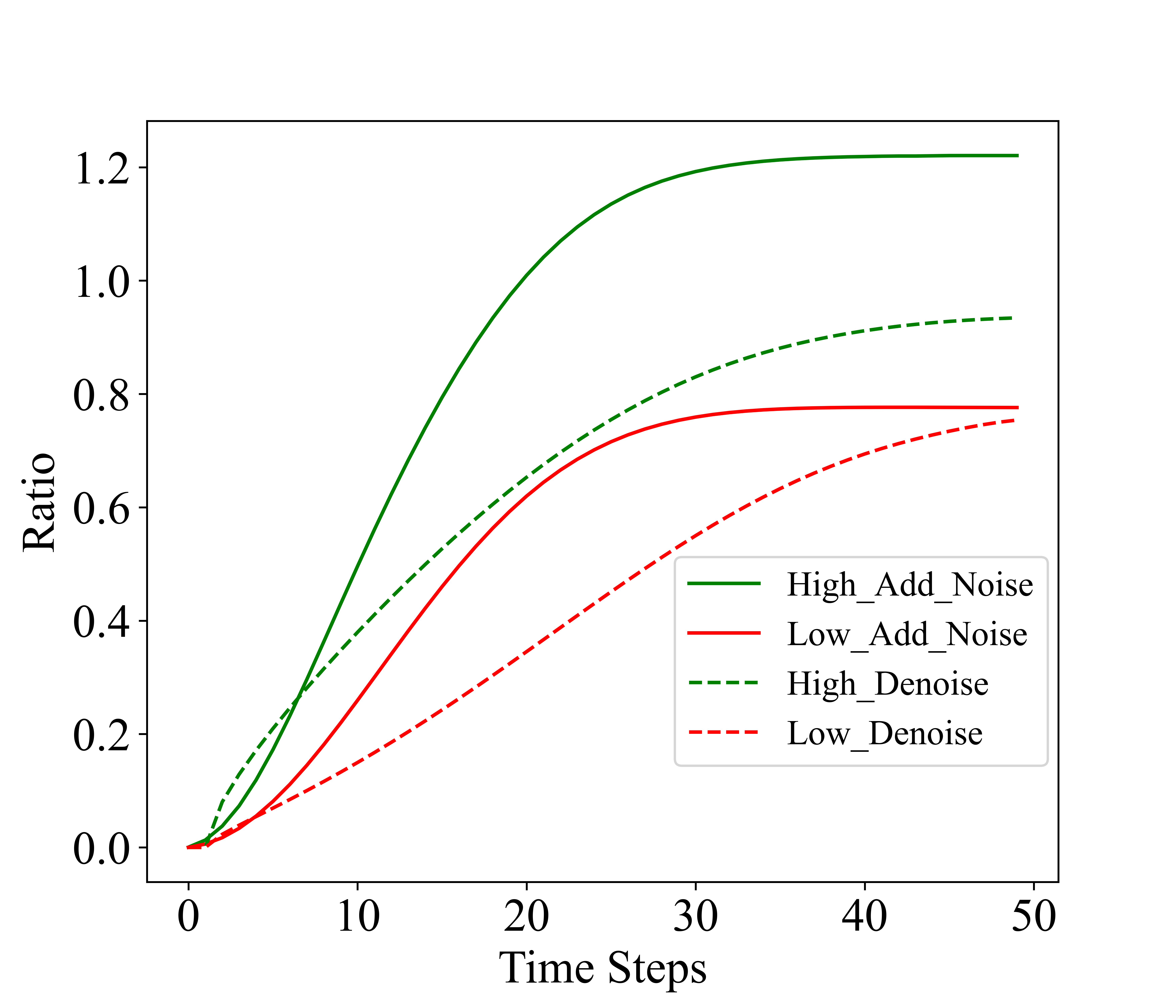
(c)

Figure 2: Figure LABEL:fig:corrupted_data visualizes the completed noisy data and its high-frequency, and low-frequency parts over different time steps, listed from top to bottom. Figures LABEL:fig:norm and LABEL:fig:ratio measure the low/high-frequency signals of $\boldsymbol{x}_{t}$. In Figure LABEL:fig:norm, “Low_Add_Noisy_Data/eps” means the norm of $\sqrt{\bar{\alpha}_{t}}\boldsymbol{x}_{0}^{\rm low}$ and $\sqrt{1-\bar{\alpha}_{t}}\boldsymbol{\epsilon}_{t}^{\rm low}$, vise versa for “High_…”. On the other hand, Figure LABEL:fig:ratio measures the variation ratio of high/low frequency parts of images during the noising/denoising process. For example, “High_Add_Noise” represents $\|\boldsymbol{x}_{t}^{\rm high}-\boldsymbol{x}_{0}^{\rm high}\|/\|\boldsymbol{x}_{0}^{\rm high}\|$ during noising process.

To further explain the above phenomenon, we refer to the frequency-signal analysis. It has been well explored that the low-frequency signals represent the overall smooth areas or slowly varying components of an image (related to the overall shape). On the other hand, the high-frequency signals correspond to the fine details or rapid changes in intensity (related to attributes like textures) [9]. Thereafter, to explain the “first overall shape then details” in the denoising process, it is natural to refer to the variations in frequency signals of images during the denoising process.

Mathematically, suppose the clean data (image latent) $\boldsymbol{x}_{0}$ has $M\times N$ dimensions for each channel with $\boldsymbol{x}_{t}$ defined in (1). Then the Fourier transformation $F_{\boldsymbol{x}_{t}}(u,v)$ (with $u\in[M],v\in[N]$) of $\boldsymbol{x}_{t}$ is

$$F_{\boldsymbol{x}_{t}}(u,v) =\frac{1}{MN}\sum\limits_{k=0}^{M-1}\sum\limits_{l=0}^{N-1}\boldsymbol{x}_{t}^{kl}\exp\left(-2\pi\mathrm{i}\left(\frac{ku}{M}+\frac{lv}{N}\right)\right)$$ (6)

$$=\sqrt{\bar{\alpha}_{t}}F_{\boldsymbol{x}_{0}}(u,v)+\sqrt{1-\bar{\alpha}_{t}}F_{\boldsymbol{\epsilon}_{t}}(u,v),$$

where $\sqrt{-1}=\mathrm{i}$, and $\boldsymbol{x}_{t}^{kl}$ is the $(k,l)$ component of $\boldsymbol{x}_{t}$. As we do not now the distribution of $\boldsymbol{x}_{0}$, we explore the $F_{\boldsymbol{\epsilon}_{t}}(u,v)$ in sequel. The result is in the following proposition proved in Appendix A.

Proposition 1.

For all $u\in[M],v\in[N]$, with probability at least $1-\delta$, we have

$$\small\left\|F_{\boldsymbol{\epsilon}_{t}}(u,v)\right\|^{2}\leq\frac{1}{\sqrt{MN}}\left(1+\sqrt{8\log{\frac{2MN}{\delta}}}\right).$$ (7)

This proposition indicates that under large image size ($MN$), the strength of frequency signals (no matter low or high) of standard Gaussian are equally close to zero. Thus, the frequency signal of $\boldsymbol{x}_{0}$ in noisy data $\boldsymbol{x}_{t}$ is mainly corrupted by the shrink factor $\bar{\alpha}_{t}$ due to (6), instead of the noise in it.

However, as visualized in Figure LABEL:fig:corrupted_data , in contrast to high-frequency part of image, the image’s low-frequency parts are more robust than the ones of high-frequency. For example, for $t=20$ in Figure LABEL:fig:corrupted_data, the shape of the clock is still perceptible in the low-frequency part of the image. If this fact is generalized to image latent, then it explains the two stages of generation as observed in Section 4.1. Because the low-frequency parts are not corrupted until the end of the adding noise process. Then, it will be recovered at the beginning of the reverse denoising process.

To investigate this, in Figures LABEL:fig:norm and LABEL:fig:ratio, we plot the averaged results over time steps of variation of low/high-frequency parts in images generated by PromptSet. In these figures, $\boldsymbol{x}_{t}^{\rm low}$ is the low-frequency part of $\boldsymbol{x}_{t}$ and vice-versa for high-frequency part $\boldsymbol{x}_{t}^{\rm high}$. As can be seen, in Figure LABEL:fig:ratio, the behavior of $\boldsymbol{x}_{t}$ is similar under add/de noise processes, and the reconstruction of low-frequency signals is faster than the high-frequency signals. On the other hand, by comparing “Low_…_Data” ( $\|\sqrt{\bar{\alpha}_{t}}\boldsymbol{x}_{0}^{\rm low}\|$) and “High_…_Data” ($\|\sqrt{\bar{\alpha}_{t}}\boldsymbol{x}_{0}^{\rm high}\|$) in Figure LABEL:fig:norm, we observe the strength of high-frequency signals are significantly lower than the low-frequency signals, which seems to be a property adopted from natural image [9]. However, the relationship oppositely holds for Gaussian noise, which is implied by Proposition 1, as the frequency signals of noise $\boldsymbol{\epsilon}_{t}$ under each spectrum are all close to zero, while the high-frequency parts contain 80% spectrum, so that $\boldsymbol{\epsilon}_{t}^{\rm high}$ is larger than the $\boldsymbol{\epsilon}_{t}^{\rm low}$.

These observations explain the phenomenon “first overall shape then details”. Since the low-frequency parts of the image (decide overall shape) are not totally corrupted until the end of the noising process. Thus, they will be firstly recovered during the reverse denoising process, while the phenomenon does not hold for low-frequency parts of the image, as they are quickly corrupted during the noising process, so they will not be recovered until the end of denoising.

5 The Working Mechanism of Text Prompt

We have verified that the denoising process has two stages i.e., “first overall shape then details”. Next, we explore the working mechanism of text prompts during these stages. Our main observations are two fold, 1): The special tokens [EOS] dominate the influence of text prompt. 2): The text prompt mainly works on the first overall shape reconstruction stage of the denoising process.

5.1 [EOS] Contains More Information

In T2I diffusion, the text prompt is encoded by auto-regressive CLIP text encoder, with semantic tokens (SEM) enclosed with special tokes [SOS] and [EOS]. For such three classes of tokens, as the information in these tokens is conveyed by the cross-attention module, we first compute the averaged weights over pixels in the cross-attention map for each class. The weights are computed by taking the average over PromptSet and presented in Figure 3. As can be seen, the weights of [SOS] are significantly larger than the other classes. However, due to the CLIP text encoder is an auto-regressive model, [SOS] does not contain any semantic information. Therefore, we conclude that the influence of [SOS] is mainly adjusting the whole cross-attention map i.e., weights on the other tokens. A similar phenomenon is observed in single-modality LLM [44]. As the information of text prompt is conveyed by semantic tokens and [EOS], we will focus on them instead of [SOS] in the sequel.

As both SEM and [EOS] contain the semantic information in the text prompt, we first explore which of them has larger impact on T2I generation. To this end, we select 3000 pairs of text prompts from PromptSet (2000 pairs follow the template, the other 1000 pairs have complex prompts), where the two text prompts are represented as “[SOS] + Prompt $A$ ($B$) + [EOS]_A(B)”. For each pair, we switch their [EOS] to construct the new text prompt pairs as “[SOS] + Prompt $A$ ($B$) + [EOS]_B(A)”.

We examine the generated images under these artificially constructed text prompts (namely Switched-PromptSet (S-PromptSet)). We call $A$ from Prompt_A as “source” and $B$ from [EOS]_B as “target” for “[SOS] + Prompt $A$ + [EOS]_B”, and vice versa. For the generated images under these prompts, we measure their alignments with the source and target prompts, respectively. The used metrics are the three standard ones in measuring text-image alignment: CLIPScore [30; 10], BLIP-VQA [18; 14], and MiniGPT4-CoT [49; 14] (details are in Appendix B).

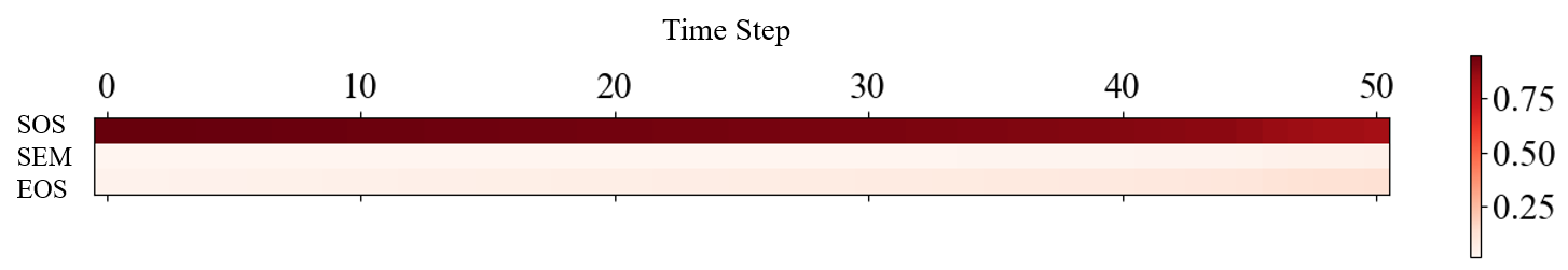
Figure 3: Averaged weights in cross-attention map over pixels of three classes of tokens. For each prompt in PromptSet, the result is obtained by taking average over tokens in each class. The final result is the average over PromptSet. Notably, the weights on [SOS] are all larger than 0.9.

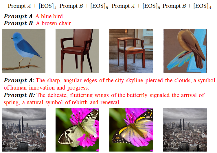
Figure 4: Images under prompts from S-PromptSet with switched [EOS]. The objects are consistent with the ones conveyed by [EOS], while some information in semantic tokens is still conveyed.

The results are in Table 1. Surprisingly, the generated images under the constructed text prompts are more likely to be aligned with the target prompt instead of the source prompt. That says, even with prefixed irrelevant semantic tokens, the information contained in [EOS] dominates the denoising process (especially for overall shape) as in Figure 4. Thus, we conclude that the special tokens [EOS] have a larger impact than semantic tokens in prompt during T2I generation. We have two speculations about this phenomenon. 1): Owing to the auto-regressive encoded text prompt, unlike semantic tokens, [EOS] contains complete textual information, so that it decides the pattern of the generated image. 2): The number of [EOS] is usually larger than semantic tokens, as the prompt is enclosed by [EOS] to length 76. An ablation study in Appendix C verifies this speculation.

In summary, our conclusion in this subsection can be summarized as: In T2I generation, the special token [EOS] decides the overall information (especially shape) of the generated image.

Remark 1.

For the generated images under S-PromptSet, we find some information in semantic tokens is also conveyed, especially for the attribute information in it, e.g., “brown” color in the last image of the first row in Figure 4. We explore this in Appendix D and explain this as: unlike noun information, attributes in semantic tokens may not conflict with the contained information in [EOS] (which quickly decides the overall shape of the generated image), so that has potential to be conveyed.

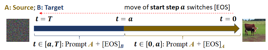
Figure 5: Desnoising process under text prompt with switched [EOS] in $[a,50]$.

Table 1: The alignment of generated image with its source and target prompts. The prompts are constructed with switched [EOS].

	Source	Target
Text-CLIPScore $\uparrow$	0.2363	0.2758
BLIP-VQA$\uparrow$	0.3325	0.4441
MiniGPT-CoT$\uparrow$	0.6473	0.7213

Figure 6: Relative text-image alignments (“current minus worst” over “best minus worst”) with source (or target) prompt under switched [EOS] (substitution in [Start Step, 50], Figure 5). Alignments with source and target prompts are respectively solid and dot lines.

5.2 The Text Prompt Mainly Working on the First Stage

In Section 4.1, we have conclude that the denoising process is divided into two stages “first overall shape then details”. Next, we explore the relationships between text prompts and the two stages. We start with special tokens [EOS] which contain major information in T2I generation. During the whole 50 denoising steps of T2I generation under prompts from S-PromptSet, we vary the starting point of substituting [EOS] i.e., the used text prompt is “[SOS] + Prompt $A$ + [EOS]_B (resp. [EOS]_A) for $t\in[\text{Start Step},50]$ (resp. $t\in[0,\text{Start Step}]$) with $\text{``Start Step''}\in[0,50]$, i.e., Figure 5. We compare the alignments of generated images with source / target prompts as in Figure 6.

In Figure 6, the alignment with the target prompt slightly decreases, until the “Start Step” of substitution close to 50. This shows that the information in [EOS] has been conveyed during the first few steps of the denoising, which is the overall shape reconstruction stage according to Section 4.

Following the revealed working stage of [EOS], we explore whether the whole text prompt also works in this stage. If so, the T2I generation will only depends on $\boldsymbol{\epsilon}_{\boldsymbol{\theta}}(t,\boldsymbol{x}_{t},\emptyset)$ in (3) for small $t$. To see this, we vary the $w$ in (3) to control the injected information from the text prompt during the denoising process. Concretely, for $a$ as the starting step of removing text prompt, i.e., during $t\in[0,a)$, we use $w=7.5$, and $w=0$ for $t\in[a,50]$, where $a\in[0,50]$. Then, the text prompt only works for $t\in[0,a)$. We generate target images $\boldsymbol{x}_{0}^{50}$ under PromptSet with standard denoising process ($a=50$), and compare them with the ones $\boldsymbol{x}_{0}^{a}$ generated under varied $a\in[0,50]$ (Figure 7). The image-image alignments are measured by standard metrics CLIPScore and $L_{1}$-distance [9]. To eliminate magnitude, we report relative results, i.e., “current minus worst” over “best minus worst”.

The results are in Figure LABEL:fig:text_prompt_influence. During generation, the text information is absence for $t\in[a,50]$, while Figure LABEL:fig:text_prompt_influence indicates that alignments between $\boldsymbol{x}_{0}^{a}$ and target $\boldsymbol{x}_{0}^{50}$ will quickly be small only for large $a$ (from 30 to 50). This shows that only if removing the textual information under large $t$, its influence to generated image is removed. Therefore, we can conclude: The information of text prompt is conveyed during the early stage of denoising process. Therefore, the overall shape of generated image is mainly decided by the text prompt, while the its details are then reconstructed by itself.

Discussion.

Next, let us explain the phenomenon. Technically, in (3), the $\boldsymbol{\epsilon}_{\boldsymbol{\theta}}(t,\boldsymbol{x}_{t},\mathcal{C},\emptyset)$ was proposed to approximate $\nabla_{\boldsymbol{x}}\log{p_{t}(\boldsymbol{x}_{t}\mid\mathcal{C})}/\sqrt{1-\bar{\alpha}_{t}}$ with decomposition ($p_{t}$ is the density of $\boldsymbol{x}_{t}$)

$$\small\nabla_{\boldsymbol{x}}\log{p_{t}(\boldsymbol{x}_{t}\mid\mathcal{C})}=\nabla_{\boldsymbol{x}}\log{p_{t}(\boldsymbol{x}_{t})}+\nabla_{\boldsymbol{x}}\log{p_{t}(\mathcal{C}\mid\boldsymbol{x}_{t})}.$$ (8)

Comparing (3) and (8), it holds $\boldsymbol{\epsilon}_{\boldsymbol{\theta}}(t,\boldsymbol{x}_{t},\emptyset)\propto\nabla_{\boldsymbol{x}}\log{p_{t}(\boldsymbol{x}_{t})}$ and $w(\boldsymbol{\epsilon}_{\boldsymbol{\theta}}(t,\boldsymbol{x}_{t},\mathcal{C})-\boldsymbol{\epsilon}_{\boldsymbol{\theta}}(t,\boldsymbol{x}_{t},\emptyset))\propto\log{p_{t}(\mathcal{C}\mid\boldsymbol{x}_{t})}$. From [37], the denoising process (4) aims to maximize log-likelihood $\log{p_{0}(\boldsymbol{x}_{0}\mid\mathcal{C})}$. Then, moving along the direction $\nabla_{\boldsymbol{x}}\log{p_{t}(\mathcal{C}\mid\boldsymbol{x}_{t})}$ (leads to large $\log{p_{t}(\mathcal{C}\mid\boldsymbol{x}_{t})}$) push $\boldsymbol{x}_{t}$ to be aligned with the text prompt $\mathcal{C}$ during the decreasing of $t$. Adding such a moving direction is standard in conditional generation [25; 36; 8; 24]. As shown in Figure LABEL:fig:noise_norm, during the denoising process, $\boldsymbol{x}_{t}$ will gradually to be consistent with $\mathcal{C}$, so that $\nabla\log{p_{t}(\mathcal{C}\mid\boldsymbol{x}_{t})}$ will decrease with $t$. Thereafter, we observe the impact of text prompt conveyed by this term decreases with $t\to 0$. Notably, owing to the quickly reconstructed overall shape of image in Section 4, the generated $\boldsymbol{x}_{t}$ will quickly be consistent with $\mathcal{C}$, so that explain the quickly decreasing $\nabla\log{p_{t}(\mathcal{C}\mid\boldsymbol{x}_{t})}$.

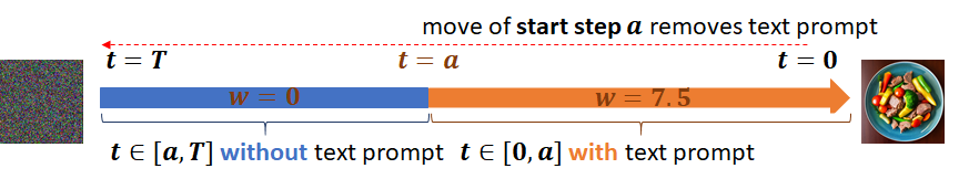
Figure 7: Desnoising with text prompt injected in $[0,a]$.

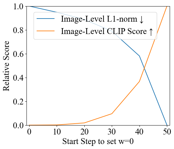
(a)

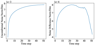
(b)

Figure 8: Figure LABEL:fig:text_prompt_influence is the relative difference “current minus worst” over “best minus worst” under different start step $a$ of Denoising process Figure 7. The last two figures LABEL:fig:noise_norm are per-dimensional norm of unconditional noise $\boldsymbol{\epsilon}_{\boldsymbol{\theta}}(t,\boldsymbol{x}_{t},\emptyset)$ and noise difference $w\left(\boldsymbol{\epsilon}_{\boldsymbol{\theta}}(t,\boldsymbol{x}_{t},\mathcal{C})-\boldsymbol{\epsilon}_{\boldsymbol{\theta}}(t,\boldsymbol{x}_{t},\emptyset)\right)$

6 Application

Acceleration of Sampling.

Since the information contained in text prompt is mainly conveyed by the noise prediction with condition $\boldsymbol{\epsilon}_{\boldsymbol{\theta}}(t,\boldsymbol{x}_{t},\mathcal{C})$, we can consider removing the evaluation of after the first few steps of denoising process. This is because the information in text prompt has been conveyed in this stage, and the computational cost can be significantly reduced without evaluating $\boldsymbol{\epsilon}_{\boldsymbol{\theta}}(t,\boldsymbol{x}_{t},\mathcal{C})$.

Therefore, we substitute the noise prediction $\boldsymbol{\epsilon}_{\boldsymbol{\theta}}(t,\boldsymbol{x}_{t},\mathcal{C},\emptyset)$ as

$$\small\boldsymbol{\epsilon}_{\boldsymbol{\theta}}(t,\boldsymbol{x}_{t},\mathcal{C},\emptyset)=\begin{dcases}\boldsymbol{\epsilon}_{\boldsymbol{\theta}}(t,\boldsymbol{x}_{t},\emptyset)+w\left(\boldsymbol{\epsilon}_{\boldsymbol{\theta}}(t,\boldsymbol{x}_{t},\mathcal{C})-\boldsymbol{\epsilon}_{\boldsymbol{\theta}}(t,\boldsymbol{x}_{t},\emptyset)\right)\qquad&a\leq t;\\ \boldsymbol{\epsilon}_{\boldsymbol{\theta}}(t,\boldsymbol{x}_{t},\emptyset)\qquad&0\leq t<a.\end{dcases}$$ (9)

By varying $a\to T$ in (9), the inference cost is reduced as an evaluation of $\boldsymbol{\epsilon}_{\boldsymbol{\theta}}(t,\boldsymbol{x}_{t},\mathcal{C})$ is saved.

To evaluate the saved computational cost of using noise prediction (9) during inference and the quality of generated data, we consider applying it on two standard samplers DDIM [36] and DPM-Solver [22] on a benchmark dataset MS-COCO [20] in T2I generation. We consider backbone models Stable-Diffusion (SD) v1.5-Base, SD v2.1-Base [31], and Pixart-Alpha [5]. Concretely, we apply noise prediction (9) with varied $a$ to generate 30K images from 30K text prompts in the test set of MS-COCO, for each sampler and backbone model. We compare the difference (measured by $L_{1}$-distance and Image-Level CLIPScore) between the generated images under $a>0$ and $a=0$ (the standard noise prediction). The results are in Table 2, where we also report the Frechet Inception Distance (FID) score [11] under each $a$ to evaluate the quality of generated images.

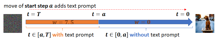
Figure 9: Desnoising under $\boldsymbol{\epsilon}_{\boldsymbol{\theta}}$ (9). The text prompt is injected in $[a,T]$, instead of $[0,a]$ in Figure 7.

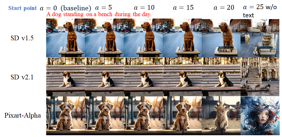
Figure 10: The generated images with 25 steps DPM-Solver under $\boldsymbol{\epsilon}_{\boldsymbol{\theta}}$ in (9) (Figure 9). The textual information is removed during $t\in[0,a]$. With $a\to 25$, the inference cost is decreased.

The Table 2 indicates that proper $a$ in (9) significantly reduces the computation cost during the inference stage without deteriorate the quality of generated images. For example, SD v1.5 with $a=20$ saves 27+% computational cost, but generates images close to the baseline method ($a=0$).

Table 2: The difference between images generated under varied $a$ with the ones of $a=0$. The results are averaged over 30K generated images, and saved latency is evaluated on one NVIDIA V100 GPU.

Start point $a$	0 (baseline)	10	20	30	40	50	0 (baseline)	5	10	15	20	25
Sampler / Backbone	DDIM / SD v1.5						DPM-Solver / SD v1.5
Image-CLIPScore $\uparrow$	1.000	0.998	0.996	0.971	0.838	0.539	1.000	0.999	0.994	0.956	0.798	0.533
$L_{1}$-distance $\downarrow$	0.000	0.011	0.022	0.043	0.087	0.195	0.000	0.015	0.027	0.050	0.100	0.188
Saved Latency $\uparrow$	0.00%	7.84%	18.10%	27.18%	35.24%	48.47%	0.00%	8.36%	17.95%	26.11%	34.86%	47.60%
FID $\downarrow$	13.772	13.770	13.805	14.012	15.048	19.296	14.297	14.286	14.725	14.985	15.860	19.758
Text-CLIPScore $\uparrow$	31.040	31.001	30.894	30.493	28.172	16.682	30.992	30.891	30.772	30.205	26.843	16.721
Sampler / Backbone	DDIM / SD v2.1						DPM-Solver / SD v2.1
Image-CLIPScore $\uparrow$	1.000	0.999	0.998	0.986	0.902	0.550	1.000	0.999	0.998	0.988	0.901	0.543
$L_{1}$-distance $\downarrow$	0.000	0.017	0.041	0.077	0.152	0.386	0.000	0.026	0.046	0.083	0.160	0.369
Saved Latency $\uparrow$	0.00%	8.68%	18.95%	28.16%	36.19%	47.99%	0.00%	8.75%	18.28%	26.24%	35.48%	47.75%
FID $\downarrow$	13.014	13.011	13.046	13.247	14.242	18.472	13.507	13.500	13.914	14.159	15.015	18.983
Text-CLIPScore $\uparrow$	31.413	31.405	31.362	31.113	29.717	16.706	31.339	31.326	31.292	31.045	29.653	16.639
Sampler / Backbone	DDIM / Pixart-Alpha						DPM-Solver / Pixart-Alpha
Image-CLIPScore $\uparrow$	1.000	0.999	0.935	0.744	0.643	0.522	1.000	0.999	0.993	0.911	0.648	0.625
$L_{1}$-distance $\downarrow$	0.000	0.024	0.058	0.103	0.169	0.247	0.000	0.013	0.022	0.046	0.098	0.199
Saved Latency $\uparrow$	0.00%	8.24%	17.98%	27.20%	34.95%	49.15%	0.00%	7.92%	15.77%	25.18%	33.80%	48.10%
FID $\downarrow$	22.651	22.884	23.258	25.485	29.760	36.525	18.669	18.520	18.798	19.358	20.494	26.159
Text-CLIPScore $\uparrow$	28.157	27.979	25.719	19.640	14.986	14.586	30.733	30.721	30.745	29.416	20.629	14.928

7 Conclusion

In this paper, we investigate the working mechanism of T2I diffusion model. By empirical and theoretical (frequency) analysis, we conclude that the denoising process firstly constructs the overall shape then details of the generated image. Next, we explore the working mechanism of text prompts. We find its special token [EOS] has a significant impact on the overall shape in the first stage of the denoising process, in which the information in the text prompt is conveyed. Then, the details of images are mainly reconstructed by themselves in the latter stage of generation. Finally, we apply our conclusion to accelerate the inference of T2I generation, and save 25%+ computational cost.

Appendix A Proofs of Proposition 1

See 1

Proof.

Note that $\boldsymbol{\epsilon}_{t}^{kl}$ (abbreviated as $\boldsymbol{\epsilon}^{kl}$) are i.i.d. Gaussian random variable for each of $k,l$. Thus we have

$$F_{\boldsymbol{\epsilon}}(u,v)=\frac{1}{MN}\sum\limits_{k=0}^{M-1}\sum\limits_{l=0}^{N-1}\boldsymbol{\epsilon}^{kl}\exp\left(-2\pi\mathrm{i}\left(\frac{ku}{M}+\frac{lv}{N}\right)\right)=\frac{1}{MN}\sum\limits_{k=0}^{M-1}\sum\limits_{l=0}^{N-1}\boldsymbol{\epsilon}^{kl}\exp\left(-\mathrm{i}\theta^{kl}_{uv}\right),$$ (10)

with $\theta^{kl}_{uv}$ is the $kl$-th angle in complex value space, and we may simplify it as $\theta^{kl}$ for ease of notations.

Next, we will show the proposition is a direct consequence of the concentration inequality of Gaussian distribution. We prove our results under one-dimensional Fourier transformation under dimension $M$, where the proof can be easily generalized to a two-dimensional case. Owing to the definition of the norm of complex value, for any specific $u$,

$$\left\|F_{\boldsymbol{\epsilon}}(u)\right\|^{2}=F_{\boldsymbol{\epsilon}}(u)\overline{F_{\boldsymbol{\epsilon}}(u)}=\frac{1}{M^{2}}\boldsymbol{\epsilon}^{\top}\Lambda\textbf{1}\textbf{1}^{\top}\bar{\Lambda}\boldsymbol{\epsilon},$$ (11)

where $\Lambda=\mathsf{diag}(e^{-i\theta^{0}},\cdots,e^{-i\theta^{M-1}})$. Then let $\boldsymbol{P}=(\sqrt{1/M}\textbf{1}^{\top},\cdots,)^{\top}\bar{\Lambda}$, where $(\sqrt{1/M}\textbf{1}^{\top},\cdots,)^{\top}$ is constructed by vector $\sqrt{1/M}\textbf{1}$ and its orthogonal complement. We can verify that $\boldsymbol{P}$ is an orthogonal matrix. Then, let $\boldsymbol{y}=\boldsymbol{P}\boldsymbol{\epsilon}$, so that $\boldsymbol{y}$ has the same distribution with $\boldsymbol{\epsilon}$. Thus

$$\small\frac{1}{M^{2}}\boldsymbol{\epsilon}^{\top}\Lambda\textbf{1}\textbf{1}^{\top}\bar{\Lambda}\boldsymbol{\epsilon}=\frac{1}{M^{2}}\boldsymbol{y}^{\top}\boldsymbol{P}\Lambda\textbf{1}\textbf{1}^{\top}\bar{\Lambda}\bar{\boldsymbol{P}}^{\top}\bar{\boldsymbol{y}}=\frac{1}{M}\boldsymbol{e}_{1}^{\top}\boldsymbol{y}\bar{\boldsymbol{y}}^{\top}\boldsymbol{e}_{1}=\frac{1}{M}(\boldsymbol{y}^{1})^{2},$$ (12)

where $\boldsymbol{y}^{1}$ is a standard Gaussian. Thus, by the Berstein’s inequality to sub-exponential random variable i.e., $\chi_{1}^{2}$, we have

$$\small\mathbb{P}\left(\left|F_{\boldsymbol{\epsilon}}(u)-\mathbb{E}\left[F_{\boldsymbol{\epsilon}}(u)\right]\right|\geq\delta\right)=\mathbb{P}\left(\left|(\boldsymbol{y}^{1})^{2}-\mathbb{E}\left[\left(\boldsymbol{y}^{1}\right)^{2}\right]\right|\geq\delta\right)\leq 2\exp\left(-\frac{1}{8}\min\left\{\delta^{2},\delta\right\}\right).$$ (13)

Since $\delta\in(0,1)$. Thus with probability at least $1-\delta/M$, we have

$$\small\frac{1}{M}-\frac{1}{M}\sqrt{8\log{\frac{2M}{\delta}}}\leq\left\|F_{\boldsymbol{\epsilon}}(u)\right\|^{2}\leq\frac{1}{M}+\frac{1}{M}\sqrt{8\log{\frac{2M}{\delta}}},$$ (14)

which proves our conclusion. ∎

Appendix B Text-Image Alignment Metrics

In this paper, we mainly use three metrics as in [14] to measure the alignment between text prompt condition and generated image. Next, we give a brief introduction to the these metrics.

CLIPScore (Text).

After extracting the features of generated images and text prompt respectively by CLIP encoder [30], CLIPScore (Text) is the cosine similarity between the two features. Similarly, the CLIPScore (Image) is the cosine-similarity between two image features.

BLIP-VQA.

To improve the limited details capturing capability of the CLIP encoder, [14] propose BLIP-VQA which leverages the visual question answering (VQA) ability of BLIP model [18]. They compare the generated with the target text prompt separately described by several questions. For example, the prompt “A blue bird” can be separated into questions “a bird ?”, “a blue bird ?” etc. Then BLIP-VQA outputs the probability of “Yes” when comparing generated images and these questions.

MiniGPT4-CoT.

The MiniGPT4-CoT [14] combines a strong multi-modality question answering model MiniGPT-4 [49] and Chain-of-Thought [43]. The metric is computed by feeding the generated images to MiniGPT-4, then sequentially asking the model two questions “describe the image” and “predict the image-text alignment score”. By constructing such CoT, the multi-modal model will not ignore the details in generated images.

Appendix C Ablation Study on Number of [EOS]

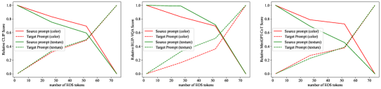
Figure 11: Relative BLIP-VQA Combine color and texture add complex, CLIP score, MiniGPT-CoT with source (or target) prompt under different number of [EOS]. Here the y-axis is the current BLIP-VQA, CLIP, MiniGPT-CoT over the maximum ones, which is used to alleviate the bias brought by the metric itself.

In this section, we conduct an ablation on the number of [EOS]. Concretely, for each text prompt in S-PromptSet, we repeat the semantic tokens in the text prompt e.g., “[SOS] + a yellow cat a yellow … + [EOS]”, so that the number of [EOS] is reduced in these constructed text prompts. Then, we generate images under these reconstructed text prompts and compare the text-image alignments between generated images and source or target prompts.

The results are in Figure 11. As can be seen, with the increasing of semantic tokens (so that decreasing of [EOS]), the generated images tend to be consistent with the source prompt, instead of the target prompt. Therefore, we speculate that the domination of [EOS] may be partially originated from its larger number, compared with semantic tokens. On the other hand, we observe that [EOS] in the forward positions have larger impacts compared to the latter ones, as the alignments between generated images with target prompts significantly decreased along the x-axis from right to left, in Figure 11. This trends further indicate that the [EOS] may contain more information compared with the latter ones, which indicates the domination of [EOS] originates from their larger number, but also the more information in the first few [EOS].

Appendix D Conveyed Information in Semantic Tokens

During our discussion in Section 5, we conclude that the [EOS] has a larger impact than the ones of semantic tokens during T2I generation. However, as observed in Figure 4, under text prompt with switched [EOS], some information in semantic tokens are still conveyed in the generated images, e.g., blue color in the last image of the first row in Figure 4. Therefore, we explore how this information is conveyed in this section, which also reveals the working mechanism of text prompt.

Firstly, in Figure 12, we visualize the cross-attention map of each tokens under text prompt from S-PromptSet, similar to Figure LABEL:fig:cross-attention_map_ratio. Surprisingly, we find that in cross-attention map of semantic tokens and [EOS] are all visually similar to the shape of the final generated images. The similarity is reasonable for [EOS] as it contains the overall information, so that it is perceptible and transfer their information according to constructed cross-attention map.

On the other hand, when semantic tokens convey their information according to the similar cross-attention, for attributes (color or texture), unlike object information, they are potentially not contradict to overall shape decided by [EOS]. Thus, the information of attributes is more likely to be conveyed in its corresponding pixels. However, this does hold for object/noun tokens whose information is very likely related to shape, which has already been decided by [EOS].

This discussion explains the phenomenon of information in semantic tokens are appeared in the generated images under prompt from S-PromptSet. Combining the observations to the working stage of text prompt in Section 5, we can conclude that the semantic tokens also work in the T2I generation, though it has less impact compared to [EOS].

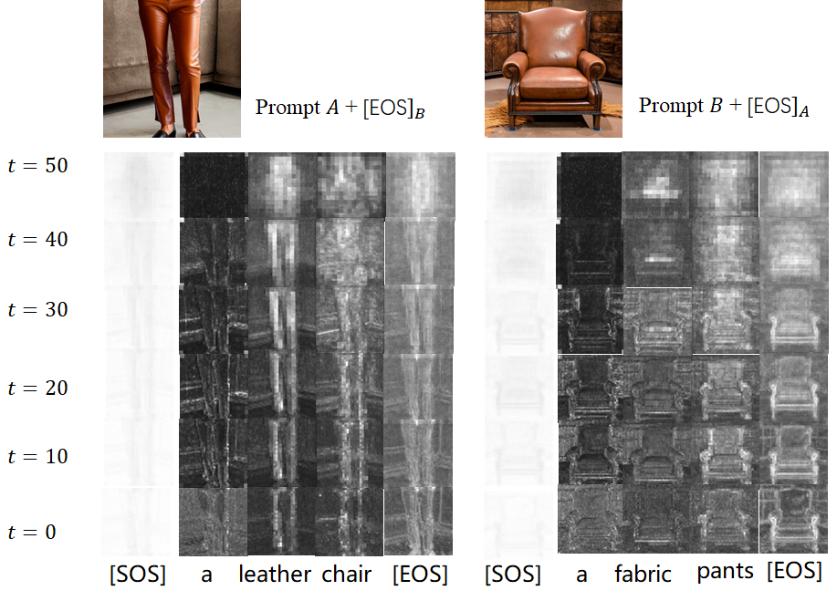
Figure 12: The visualization of cross-attention map under text prompt with switched [EOS] from S-PromptSet. The pixels corresponding to semantic tokens are in the shape of the final generated data as in text prompt $B$ provide [EOS]. For example, the token “chair” corresponds to pixels in the shape of paint, so its information can not be conveyed, while this phenomenon does exist in the attribute token “leather”.

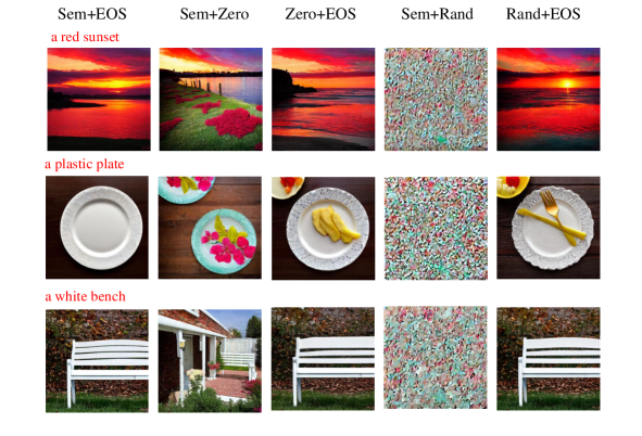
Figure 13: Generated images with zero or random vectors substitution.

Appendix E More Evidences on [EOS] Contains More Information

Table 3: The alignment of generated results image under different constructed text prompt sets. Here “Sem + EOS” is the original text prompt, and serves as baseline here. Besides that, the CLIPScore (Image) is the image-level alignment of generated images with the ones under “Sem + EOS”.

Text Prompt	CLIPScore (Text)$\uparrow$	CLIPScore (Image)$\uparrow$	BLIP-VQA$\uparrow$	MiniGPT4-CoT$\uparrow$
Sem + Zero	0.2407	0.6732	0.5392	0.6757
Sem + Rand	0.2153	0.6038	0.3606	0.5428
Zero + EOS	0.2999	0.8887	0.7467	0.6982
Rand + EOS	0.3008	0.8791	0.7669	0.7000
Sem + EOS	0.3110	1.0000	0.8999	0.7412

In this section, we further verify that the impact of [EOS] is larger than the ones of semantic tokens in T2I generation. To further verify this conclusion, under the text prompts with the format of “[SOS] + Sem + [EOS]” from our dataset PromptSet, we substitute all semantic tokens or [EOS] with zero vectors or random Gaussian noise. As a result, we get the 4 sets of text prompts, i.e., “[SOS] + Sem + Zero” (abbrev Sem + Zero), “[SOS] + Sem + Random” (Sem + Rand), “[SOS] + Zero + [EOS]” (Zero + EOS), and “[SOS] + Random + [EOS]” (Rand + EOS). These constructed text prompts ideally contain complete semantic information, and we verify the alignment of the generated images with the corresponding text prompt conditions. The alignments are measured by text-image alignment metrics: CLIPScore [30, 10], BLIP-VQA [18, 14], and MiniGPT4-CoT [49, 14].

The results are summarized in Table 3. As can be seen, as expected for baseline combination “Sem + EOS”, the alignments under text prompts with “EOS” preserved are significantly better than the ones with “Sem” preserved. Thus, the observations further verify our conclusion that the [EOS] has larger influences than semantic tokens during the denoising process.

Moreover, we find the generation is somehow robust, as involving random noise in text prompts still generates semantic meaningful images. We visualize some generated images under constructed text-prompts from Table 3 in Figure 13, which indicates the images under “Zero + EOS” indeed visually have the best quality in alignment, so that consist with Table 3. Besides that, the other combinations generate semantic meaningful images as well, expected for “Sem + Rand” Thus semantic tokens do not contain enough information for generation.

Appendix F Key or Value Dominates the Influence?

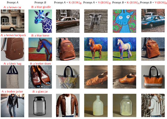
Figure 14: Generated examples of Key or Value substitution.

Figure 15: The averaged KL-divergence over pixels and layers.

Table 4: The alignment of generated image with its source and target prompts, under switched [EOS] on Key or Value substitution. Here $KV$-Sub is the complete substitution as in Section 5, which serves as a baseline here.

	$K$-Sub		$V$-Sub		$KV$-Sub
	Source	Target	Source	Target	Source	Target
CLIPScore (Text)$\uparrow$	0.3132	0.1875	0.2538	0.2628	0.2363	0.2758
BLIP-VQA$\uparrow$	0.7127	0.2379	0.3724	0.3984	0.3325	0.4441
MiniGPT-CoT$\uparrow$	0.8025	0.6215	0.6749	0.7071	0.6473	0.7213

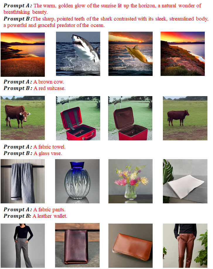
Figure 16: More generated examples under tokens from S-PromptSet.

As mentioned in Section 3, the information from [EOS] is conveyed by the cross-attention module. More concretely, the Key ($K$) and Value ($V$) in it, respectively decide the weights and features in the output of the cross-attention module (a weighted sum of features). Next, we explore their individual influence for [EOS] to further reveal the working mechanism of it.

Concretely, as in Section 5, we generate images under the constructed text prompt set S-PromptSet. However, the substitution of [EOS] is only conducted on computing Key or Values in cross-attention module, which are respectively denoted as $K$-Substitution (Sub) and $V$-Sub. For such two substitutions, similar to Table 1, we compare the image-text alignment of generated images with source and target prompts.

The results are summarized in Table 4. As can be seen, substituting the [EOS] in $V$ has a larger influence than the substitutions in $K$. To explain this, as we have observed in Figure 3, the weights on semantic tokens and [EOS] are significantly smaller than the ones on [SOS]. However, the $K$ of [EOS] is only related to these small weights, which have limited influence. In contrast to $K$, the $V$ of [EOS] contains information on features, which can be directly conveyed in generated images. So that we can conclude the value of [EOS] dominates the influence in generation as observed in Table 4. We present some generated images under text prompts from S-PromptSet, but with only Key or Value substituted as in Table 4. The generated images are in Figure 14.

We further verify the variation of the cross-attention map after substituting [EOS]. For each pixel, the cross-attention map of it is a discrete probability distribution. Thus, we compute the KL-divergence [41] between probability distributions under substituted/unsubstituted $K$. The averaged KL-divergence over pixels and layers in models under different denoising steps is presented in Figure 15, where we add the KL-divergence of cross-attention map distribution between a uniform distribution as a baseline. The result shows that even with substituted [EOS], the cross-attention map does not vary much. We speculate that this is because as in Figure 3, the weights in [SOS] dominate the cross-attention map. Thus, in the cross-attention module, altering $K$ has a slighter influence compared with altering $V$.

Appendix G More Generated Images

In this section, we present more generated images.

G.1 [EOS] Substitution

In this subsection, we first present the generated images under text prompts from S-PromptSet in Figure 16. As can be seen, most overall shape of generated images are consistent with the ones conveyed by [EOS].

G.2 Generated Images in Paragraph “Acceleration of Sampling” of Section 6

In this subsection, we present more generated images under noise prediction (9) with varied $a$. The results are in Figure 17 and 18.

Figure 17: The generated images with 50 steps DDIM under $\boldsymbol{\epsilon}_{\boldsymbol{\theta}}$ in (9), where the textual information are $\mathcal{C}$ removed during time steps $t\in[0,a]$. With $a\to 50$, the inference cost is decreased.

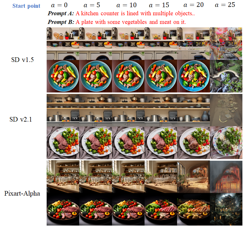
Figure 18: More generated images with 25 steps DPM-Solver under $\boldsymbol{\epsilon}_{\boldsymbol{\theta}}$ in (9), where the textual information are $\mathcal{C}$ removed during time steps $t\in[0,a]$. With $a\to 25$, the inference cost is decreased.

References

- [1] Yogesh Balaji, Seungjun Nah, Xun Huang, Arash Vahdat, Jiaming Song, Karsten Kreis, Miika Aittala, Timo Aila, Samuli Laine, Bryan Catanzaro, et al. ediffi: Text-to-image diffusion models with an ensemble of expert denoisers. Preprint arXiv:2211.01324, 2022.
- [2] Fan Bao, Shen Nie, Kaiwen Xue, Yue Cao, Chongxuan Li, Hang Su, and Jun Zhu. All are worth words: A vit backbone for diffusion models. In Conference on Computer Vision and Pattern Recognition, 2023.
- [3] Tom Brown, Benjamin Mann, Nick Ryder, Melanie Subbiah, Jared D Kaplan, Prafulla Dhariwal, Arvind Neelakantan, Pranav Shyam, Girish Sastry, Amanda Askell, et al. Language models are few-shot learners. 2020.
- [4] Wenhao Chai, Xun Guo, Gaoang Wang, and Yan Lu. Stablevideo: Text-driven consistency-aware diffusion video editing. In International Conference on Computer Vision, 2023.
- [5] Junsong Chen, YU Jincheng, GE Chongjian, Lewei Yao, Enze Xie, Zhongdao Wang, James Kwok, Ping Luo, Huchuan Lu, and Zhenguo Li. Pixart-alpha: Fast training of diffusion transformer for photorealistic text-to-image synthesis. In International Conference on Learning Representations, 2024.
- [6] Florinel-Alin Croitoru, Vlad Hondru, Radu Tudor Ionescu, and Mubarak Shah. Diffusion models in vision: A survey. IEEE Transactions on Pattern Analysis and Machine Intelligence, 2023.
- [7] Patrick Esser, Robin Rombach, and Bjorn Ommer. Taming transformers for high-resolution image synthesis. In Conference on Computer Vision and Pattern Recognition, 2021.
- [8] Karim Farid, Simon Schrodi, Max Argus, and Thomas Brox. Latent diffusion counterfactual explanations. Preprint arXiv:2310.06668, 2023.
- [9] Rafael C Gonzales and Paul Wintz. Digital image processing. Addison-Wesley Longman Publishing Co., Inc., 1987.
- [10] Jack Hessel, Ari Holtzman, Maxwell Forbes, Ronan Le Bras, and Yejin Choi. Clipscore: A reference-free evaluation metric for image captioning. In Conference on Empirical Methods in Natural Language Processing, 2021.
- [11] Martin Heusel, Hubert Ramsauer, Thomas Unterthiner, Bernhard Nessler, and Sepp Hochreiter. Gans trained by a two time-scale update rule converge to a local nash equilibrium. 2017.
- [12] Jonathan Ho, Ajay Jain, and Pieter Abbeel. Denoising diffusion probabilistic models. In Advances in Neural Information Processing Systems, 2020.
- [13] Jonathan Ho and Tim Salimans. Classifier-free diffusion guidance. In NeurIPS 2021 Workshop on Deep Generative Models and Downstream Applications, 2021.
- [14] Kaiyi Huang, Kaiyue Sun, Enze Xie, Zhenguo Li, and Xihui Liu. T2i-compbench: A comprehensive benchmark for open-world compositional text-to-image generation. In Conference on Neural Information Processing Systems Datasets and Benchmarks Track, 2023.
- [15] Minguk Kang, Jun-Yan Zhu, Richard Zhang, Jaesik Park, Eli Shechtman, Sylvain Paris, and Taesung Park. Scaling up gans for text-to-image synthesis. In Conference on Computer Vision and Pattern Recognition, 2023.
- [16] Kalpesh Krishna, Yapei Chang, John Wieting, and Mohit Iyyer. Rankgen: Improving text generation with large ranking models. In Empirical Methods in Natural Language Processing, 2022.
- [17] Junnan Li, Dongxu Li, Silvio Savarese, and Steven Hoi. Blip-2: Bootstrapping language-image pre-training with frozen image encoders and large language models. Preprint arXiv:2301.12597, 2023.
- [18] Junnan Li, Dongxu Li, Caiming Xiong, and Steven Hoi. Blip: Bootstrapping language-image pre-training for unified vision-language understanding and generation. In International Conference on Machine Learning, 2022.
- [19] Chen-Hsuan Lin, Jun Gao, Luming Tang, Towaki Takikawa, Xiaohui Zeng, Xun Huang, Karsten Kreis, Sanja Fidler, Ming-Yu Liu, and Tsung-Yi Lin. Magic3d: High-resolution text-to-3d content creation. In Conference on Computer Vision and Pattern Recognition, 2023.
- [20] Tsung-Yi Lin, Michael Maire, Serge Belongie, James Hays, Pietro Perona, Deva Ramanan, Piotr Dollár, and C Lawrence Zitnick. Microsoft coco: Common objects in context. In European Conference on Computer Vision, 2014.
- [21] Nelson F Liu, Kevin Lin, John Hewitt, Ashwin Paranjape, Michele Bevilacqua, Fabio Petroni, and Percy Liang. Lost in the middle: How language models use long contexts. Preprint arXiv:2307.03172, 2023.
- [22] Cheng Lu, Yuhao Zhou, Fan Bao, Jianfei Chen, Chongxuan Li, and Jun Zhu. Dpm-solver: A fast ode solver for diffusion probabilistic model sampling in around 10 steps. In Advances in Neural Information Processing Systems, 2022.
- [23] Timo Lüddecke and Alexander Ecker. Image segmentation using text and image prompts. In Conference on Computer Vision and Pattern Recognition, 2022.
- [24] Nishtha Madaan, Inkit Padhi, Naveen Panwar, and Diptikalyan Saha. Generate your counterfactuals: Towards controlled counterfactual generation for text. In Association for the Advancement of Artificial Intelligence, 2021.
- [25] Petr Marek, Vishal Ishwar Naik, Anuj Goyal, and Vincent Auvray. Oodgan: Generative adversarial network for out-of-domain data generation. In Conference of the North American Chapter of the Association for Computational Linguistics, 2021.
- [26] Eyal Molad, Eliahu Horwitz, Dani Valevski, Alex Rav Acha, Yossi Matias, Yael Pritch, Yaniv Leviathan, and Yedid Hoshen. Dreamix: Video diffusion models are general video editors. Preprint arXiv:2302.01329, 2023.
- [27] OpenAI. Gpt-4 technical report. Preprint arXiv:2304.10592, 2023.
- [28] William Peebles and Saining Xie. Scalable diffusion models with transformers. In International Conference on Computer Vision, 2023.
- [29] Ben Poole, Ajay Jain, Jonathan T Barron, and Ben Mildenhall. Dreamfusion: Text-to-3d using 2d diffusion. In International Conference on Learning Representations, 2022.
- [30] Alec Radford, Jong Wook Kim, Chris Hallacy, Aditya Ramesh, Gabriel Goh, Sandhini Agarwal, Girish Sastry, Amanda Askell, Pamela Mishkin, Jack Clark, et al. Learning transferable visual models from natural language supervision. In International conference on machine learning, 2021.
- [31] Aditya Ramesh, Prafulla Dhariwal, Alex Nichol, Casey Chu, and Mark Chen. Hierarchical text-conditional image generation with clip latents. Preprint arXiv:2204.06125, 2022.
- [32] Robin Rombach, Andreas Blattmann, Dominik Lorenz, Patrick Esser, and Björn Ommer. High-resolution image synthesis with latent diffusion models. In Conference on Computer Vision and Pattern Recognition, 2022.
- [33] Nataniel Ruiz, Yuanzhen Li, Varun Jampani, Yael Pritch, Michael Rubinstein, and Kfir Aberman. Dreambooth: Fine tuning text-to-image diffusion models for subject-driven generation. In Conference on Computer Vision and Pattern Recognition, 2023.
- [34] Chitwan Saharia, William Chan, Saurabh Saxena, Lala Li, Jay Whang, Emily L Denton, Kamyar Ghasemipour, Raphael Gontijo Lopes, Burcu Karagol Ayan, Tim Salimans, et al. Photorealistic text-to-image diffusion models with deep language understanding. In Advances in Neural Information Processing Systems, 2022.
- [35] Chenyang Si, Ziqi Huang, Yuming Jiang, and Ziwei Liu. Freeu: Free lunch in diffusion u-net. Preprint arXiv:2309.11497, 2023.
- [36] Jiaming Song, Chenlin Meng, and Stefano Ermon. Denoising diffusion implicit models. In International Conference on Learning Representations, 2022.
- [37] Yang Song, Jascha Sohl-Dickstein, Diederik P Kingma, Abhishek Kumar, Stefano Ermon, and Ben Poole. Score-based generative modeling through stochastic differential equations. In International Conference on Learning Representations, 2020.
- [38] Simeng Sun, Kalpesh Krishna, Andrew Mattarella-Micke, and Mohit Iyyer. Do long-range language models actually use long-range context? In Conference on Empirical Methods in Natural Language Processing, 2021.
- [39] Abdel Aziz Taha and Allan Hanbury. Metrics for evaluating 3d medical image segmentation: analysis, selection, and tool. BMC Medical Imaging, 15:29, 2015.
- [40] Raphael Tang, Akshat Pandey, Zhiying Jiang, Gefei Yang, Karun Kumar, Jimmy Lin, and Ferhan Ture. What the daam: Interpreting stable diffusion using cross attention. 2023.
- [41] Vladimir Vapnik. The nature of statistical learning theory. Springer science & business media, 1999.
- [42] Ashish Vaswani, Noam Shazeer, Niki Parmar, Jakob Uszkoreit, Llion Jones, Aidan N Gomez, Łukasz Kaiser, and Illia Polosukhin. Attention is all you need. Advances in Neural Information Processing Systems, 2017.
- [43] Jason Wei, Xuezhi Wang, Dale Schuurmans, Maarten Bosma, Fei Xia, Ed Chi, Quoc V Le, Denny Zhou, et al. Chain-of-thought prompting elicits reasoning in large language models. 2022.
- [44] Guangxuan Xiao, Yuandong Tian, Beidi Chen, Song Han, and Mike Lewis. Efficient streaming language models with attention sinks. Preprint arXiv:2309.17453, 2023.
- [45] Xingyi Yang, Daquan Zhou, Jiashi Feng, and Xinchao Wang. Diffusion probabilistic model made slim. In Conference on Computer Vision and Pattern Recognition, 2023.
- [46] Jiahui Yu, Yuanzhong Xu, Jing Yu Koh, Thang Luong, Gunjan Baid, Zirui Wang, Vijay Vasudevan, Alexander Ku, Yinfei Yang, Burcu Karagol Ayan, et al. Scaling autoregressive models for content-rich text-to-image generation. Transactions on Machine Learning Research, 2022.
- [47] Chiyuan Zhang, Daphne Ippolito, Katherine Lee, Matthew Jagielski, Florian Tramèr, and Nicholas Carlini. Counterfactual memorization in neural language models. Preprint arXiv:2112.12938, 2021.
- [48] Wentian Zhang, Haozhe Liu, Jinheng Xie, Francesco Faccio, Mike Zheng Shou, and Jürgen Schmidhuber. Cross-attention makes inference cumbersome in text-to-image diffusion models. Preprint arXiv:2404.02747, 2024.
- [49] Deyao Zhu, Jun Chen, Xiaoqian Shen, Xiang Li, and Mohamed Elhoseiny. Minigpt-4: Enhancing vision-language understanding with advanced large language models. Preprint arXiv:2304.10592, 2023.