Cross-Validated Off-Policy Evaluation

Abstract

In this paper, we study the problem of estimator selection and hyper-parameter tuning in off-policy evaluation. Although cross-validation is the most popular method for model selection in supervised learning, off-policy evaluation relies mostly on theory-based approaches, which provide only limited guidance to practitioners. We show how to use cross-validation for off-policy evaluation. This challenges a popular belief that cross-validation in off-policy evaluation is not feasible. We evaluate our method empirically and show that it addresses a variety of use cases.

1 Introduction

Off-policy evaluation (OPE, Li et al., , 2010) is a framework for estimating the performance of a policy without deploying it online. It is useful in domains where online A/B testing is costly or too dangerous. For example, deploying an untested algorithm in recommender systems or advertising can lead to a loss of revenue or customer trust (Li et al., , 2010; Silver et al., , 2013), and in medical treatments, it may have a detrimental effect on the patient’s health (Hauskrecht and Fraser, , 2000). A popular approach to off-policy evaluation is inverse propensity scoring (IPS, Robins et al., , 1994). As this method is unbiased, it approaches a true policy value with more data.

However, when the data logging policy has a low probability of choosing some actions, IPS-based estimates have a high variance and often require a large amount of data to be useful in practice (Dudik et al., , 2014). Therefore, other lower-variance methods have emerged. These methods often have some hyper-parameters, such as a clipping constant to truncate large propensity weights (Ionides, , 2008). Some works provide theoretical insights (Ionides, , 2008; Metelli et al., , 2021) for choosing hyper-parameters, while there are none for many others.

In supervised learning, data-driven techniques for hyper-parameter tuning, such as cross-validation, are more popular than theory-based techniques, such as the Akaike information criterion (Bishop, , 2006). The reason is that they perform better on large datasets, which are common today. Unlike in supervised learning, the ground truth value of the target policy is unknown in off-policy evaluation. A common assumption in off-policy evaluation is that standard machine learning approaches for model selection would fail because there is no unbiased and low-variance approach to compare estimators (Su et al., 2020b, ; Udagawa et al., , 2023). Therefore, only a few works studied estimator selection for off-policy evaluation, and no general solution exists (Su et al., 2020b, ; Saito et al., , 2021; Udagawa et al., , 2023).

Despite common beliefs, this work shows that cross-validation in off-policy evaluation can be done comparably to supervised learning. In supervised learning, we do not know the true data distribution, but we are given samples from it. Each sample is an unbiased and high-variance representation of this distribution. Nevertheless, we can still get an accurate estimate of true generalization when averaging the model error over these samples in cross-validation. Similarly, we do not know the true reward distribution in off-policy evaluation, but we are given high-variance samples from it. The difference is that these samples are biased because they are collected by a different policy. However, we can use an unbiased estimator, such as IPS, on a held-out validation set to get an unbiased estimate of another policy’s value. Then, similarly to supervised learning, we get an estimate of the estimator’s performance. Our contributions are:

• We propose an easy-to-use estimator selection procedure based on cross-validation that requires only data collected by a single policy.

• We analyze the procedure in an idealized setting and use this insight to reduce its variance.

• We empirically evaluate the procedure on estimator selection and hyper-parameter tuning problems using multiple real-world datasets. We show that our method is more accurate than prior techniques and computationally efficient.

2 Off-policy evaluation

A contextual bandit (Langford et al., , 2008) is a general and popular model of an agent interacting with an environment. The interaction in round $i$ starts with the agent observing a context $x_{i}\in\mathcal{X}$ drawn i.i.d. from an unknown distribution $p$, where $\mathcal{X}$ is the context set. Then the agent takes an action $a_{i}\sim\pi(\cdot\mid x_{i})$ from the action set $\mathcal{A}$ according to its policy $\pi$. Finally, it receives a stochastic reward $r_{i}=r(x_{i},a_{i})+\varepsilon_{i}$, where $r(x,a)$ is the mean reward for taking action $a$ in context $x$ and $\varepsilon_{i}$ is an independent zero-mean noise.

In off-policy evaluation (OPE, Li et al., , 2010), a logging policy $\pi_{0}$ interacts with the bandit for $N$ rounds and collects a logged dataset $\mathcal{D}=\left\{(x_{i},a_{i},r_{i})\right\}_{i=1}^{N}$. The goal is to design $\hat{V}$, an estimator of the target policy value $V(\pi)=\sum_{x\in\mathcal{X}}\sum_{a\in\mathcal{A}}p(x)\pi(a\mid x)r(x,a)$, using the logged dataset $\mathcal{D}$ such that $\hat{V}(\pi;\mathcal{D})\approx V(\pi)$. Various off-policy estimators are used to either correct for the distribution shift caused by the difference in $\pi$ and $\pi_{0}$, or to estimate $r(x,a)$. We review the canonical ones below and leave the rest for Appendix A.

The inverse propensity scores estimator (IPS, Robins et al., , 1994) reweights logged samples as if collected by the target policy $\pi$,

$$\hat{V}_{\textsc{IPS}}(\pi;\mathcal{D})=\frac{1}{N}\sum_{i=1}^{N}\frac{\pi(a_{i}\mid x_{i})}{\pi_{0}(a_{i}\mid x_{i})}r_{i}\,.$$ (1)

This estimator is unbiased but suffers from a high variance. Hence, a clipping constant was introduced to truncate high propensity weights (Ionides, , 2008). This is a hyper-parameter that needs to be tuned.

The direct method (DM, Dudik et al., , 2014) is a popular approach to off-policy evaluation. Using the DM, the policy value estimate can be computed as

$$\hat{V}_{\textsc{DM}}(\pi;\mathcal{D})=\frac{1}{N}\sum_{i=1}^{N}\sum_{a\in\mathcal{A}}\pi(a\mid x_{i})\hat{f}(x_{i},a)\,,$$ (2)

where $\hat{f}(x,a)$ is an estimate of the mean reward $r(x,a)$ from $\mathcal{D}$. The function $\hat{f}$ is chosen from some function class, such as linear functions.

The doubly-robust estimator (DR, Dudik et al., , 2014) combines the DM and IPS as

$$\hat{V}_{\textsc{DR}}(\pi;\mathcal{D})=\frac{1}{N}\sum_{i=1}^{N}\frac{\pi(a_{i}\mid x_{i})}{\pi_{0}(a_{i}\mid x_{i})}(r_{i}-\hat{f}(x_{i},a_{i}))+\hat{V}_{\textsc{DM}}(\pi;\mathcal{D})\,,$$ (3)

where $\hat{f}(x,a)$ is an estimate of $r(x,a)$ from $\mathcal{D}$. The DR is unbiased when the DM is, or the propensity weights are correctly specified. It is popular in practice because $r_{i}-\hat{f}(x_{i},a_{i})$ reduces the variance of rewards in the IPS part of the estimator.

Many other estimators with tunable parameters exist: TruncatedIPS (Ionides, , 2008), Switch-DR (Wang et al., , 2017), Continuous OPE (Kallus and Zhou, , 2018), CAB (Su et al., , 2019), DRos and DRps (Su et al., 2020a, ), IPS-$\lambda$ (Metelli et al., , 2021), MIPS (Saito and Joachims, , 2022), Exponentially smooth IPS (Aouali et al., , 2023), GroupIPS (Peng et al., , 2023), OffCEM (Saito et al., , 2023), Policy Convolution (Sachdeva et al., , 2023), and Learned MIPS (Cief et al., , 2024). Some of these works leave the hyper-parameter selection as an open problem, while others provide a theory for selecting an optimal hyper-parameter, usually by bounding the bias of the estimator. As in supervised learning, we show that theory is often too conservative, and given enough data, our method can select better hyper-parameters. Other works use the statistical Lepski’s adaptation method (Lepski and Spokoiny, , 1997), which requires that the hyper-parameters are ordered so that the bias is monotonically increasing. The practitioner also needs to choose the estimator. To address these shortcomings, we adapt cross-validation, a well-known machine learning technique for model selection, to estimator selection in a way that is general and applicable to any estimator.

3 Existing methods for estimator selection and hyper-parameter tuning

To the best of our knowledge, there are only a few data-driven approaches for estimator selection or hyper-parameter tuning in off-policy evaluation for bandits. We review them below.

Su et al., 2020b propose a hyper-parameter tuning method Slope based on Lepski’s principle for bandwidth selection in non-parametric statistics (Lepski and Spokoiny, , 1997). In Slope, we order the hyper-parameter values so that the estimator’s variance decreases as we progress through them. Then, we compute the confidence intervals for all the values in this order. If a confidence interval does not overlap with all previous intervals, we stop and select the previous value. While the method is straightforward, it assumes that the hyper-parameters are ordered such that the bias is monotonically increasing. This makes it impractical for estimator selection, where it may be difficult to establish a correct order between various estimators.

Saito et al., (2021) rely on a logged dataset collected by multiple logging policies. They use one of the logging policies as the pseudo-target policy and directly estimate its value from the dataset. Then, they choose the off-policy estimator that most accurately estimates the pseudo-target policy. This approach assumes that we have access to a logged dataset collected by multiple policies. Moreover, it ultimately chooses the best estimator for the pseudo-target policy, not the one we are interested in. Prior empirical studies (Voloshin et al., , 2021) showed that the estimator’s accuracy greatly varies when applied to different target policies.

In $\tt PAS\mathchar 45\relax IF$ (Udagawa et al., , 2023), two new surrogate policies are created using the logged dataset. The surrogate policies have two properties: 1) the propensity weights from surrogate logging and target policies imitate those of the true logging and target policies, and 2) the logged dataset can be split in two as if each part was collected by one of the surrogate policies. They learn a neural network that optimizes this objective. Then, they evaluate estimators as in Saito et al., (2021), using surrogate policies and a precisely split dataset. They show that estimator selection on these surrogate policies adapts better to the true target policy.

We do not require multiple logging policies, make no strong assumptions, and only use principal techniques from supervised learning that are well-known and loved by practitioners. Therefore, our method is easy to implement and, as shown in Section 6, also more accurate.

A popular approach in offline policy selection (Lee et al., , 2022; Nie et al., , 2022; Saito and Nomura, , 2024) is to evaluate candidate policies on a held-out set by OPE. Nie et al., (2022) even considered a similar approach to cross-validation. While these papers seem similar to our work, the problems are completely different. All estimators in our work estimate the same value $V(\pi)$, and this structure is used in the design of our solution (Section 5). We also address important questions that the prior works did not, such as what the training/validation split should be and how to choose a validator. A naive application of cross-validation fails in OPE without addressing these issues (Appendix B).

4 Cross-validation in machine learning

Model and hyper-parameter selection are classic problems in machine learning (Bishop, , 2006). There are two prevalent approaches. The first approach is probabilistic model selection, such as Akaike information criterion (Akaike, , 1998) and Bayesian information criterion (Schwarz, , 1978). These methods quantify the model performance on the training dataset and penalize its complexity (Stoica and Selen, , 2004). They are designed using theory and do not require a validation set. In general, they work well on smaller datasets because they favor simple models (Bishop, , 2006). The second approach estimates the model performance on a held-out validation set, such as cross-validation (CV, Stone, , 1974). CV is a state-of-the-art approach for large datasets and is used widely in training neural networks (Yao et al., , 2007). We focus on this setting because large amounts of logged data are available in modern machine learning.

In this section, we formalize CV, and in the following section, we apply it to off-policy evaluation. Let $f:\mathbb{R}^{d}\to\mathbb{R}$ be a function that maps features $x\in\mathbb{R}^{d}$ to $\mathbb{R}$. It belongs to some function class $\mathcal{F}$. For example, $f$ is a linear function, and $\mathcal{F}$ is the class of linear functions. A machine learning algorithm $\mathcal{M}$ maps a dataset $\mathcal{D}$ to a function in $\mathcal{F}$. We write this as $f=\mathcal{M}(\mathcal{F},\mathcal{D})$. One approach to choosing function $f$ is to minimize some loss function $L$ on the training set,

$$\mathcal{M}(\mathcal{F},\mathcal{D})=\operatorname*{arg\,min\,}_{f\in\mathcal{F}}L(f,\mathcal{D})\,,$$ (4)

where $L(f,\mathcal{D})=\frac{1}{|\mathcal{D}|}\sum_{(x,y)\in\mathcal{D}}(y-f(x))^{2}$ is the mean squared loss. This results in overfitting on the training set (Devroye et al., , 1996). Therefore, CV is commonly used to evaluate $f$ on unseen validation data to give a more honest estimate of how the model generalizes. In $K$-fold CV, the dataset is split into $K$ folds. We denote the data in the $k$-th fold used for validation by $\mathcal{D}_{k}$ and all other training data by $\mathcal{D}_{-k}$. Then the average performance on a held-out set can be formally written as $\frac{1}{K}\sum_{k=1}^{K}L(\mathcal{M}(\mathcal{F},\mathcal{D}_{-k}),\mathcal{D}_{k})$. This can be used for model selection as follows. Suppose that we have a set of function classes $\mathbf{F}=\left\{\mathcal{F}\right\}$. For instance, it can be $\mathbf{F}=\left\{\mathcal{F}_{1},\mathcal{F}_{2}\right\}$, where $\mathcal{F}_{1}$ is the set of linear functions and $\mathcal{F}_{2}$ is the set of quadratic functions. Then, the best function class under CV is

$$\mathcal{F}_{*}=\operatorname*{arg\,min\,}_{\mathcal{F}\in\mathbf{F}}\frac{1}{K}\sum_{k=1}^{K}L(\mathcal{M}(\mathcal{F},\mathcal{D}_{-k}),\mathcal{D}_{k})\,.$$ (5)

After this, the best model $f_{*}=\mathcal{M}(\mathcal{F}_{*},\mathcal{D})$ trained on the entire dataset is used.

5 Off-policy cross-validation

In this section, we show how to adapt the CV to off-policy evaluation. In supervised learning, we do not know the true data distribution but are given samples from it. Each individual sample is an unbiased but high-variance representation of the true distribution. As in supervised learning, we do not know the true value of policy $\pi$ in off-policy evaluation. However, we have samples collected by another policy $\pi_{0}$ and can obtain an unbiased estimate of $V(\pi)$ using an unbiased estimator. We define the loss of an evaluated estimator $\hat{V}$ with respect to a validation estimator $\tilde{V}$ on dataset $\mathcal{D}$ as

$$L(\hat{V},\mathcal{D})=(\tilde{V}(\pi;\mathcal{D})-\hat{V}(\pi))^{2}\,.$$ (6)

The validation estimator can be any unbiased estimator, such as $\hat{V}_{\textsc{IPS}}$ or $\hat{V}_{\textsc{DR}}$. Unlike in supervised learning, the loss is only over one observation, an unbiased estimate of $V(\pi)$. We wanted to comment on two aspects of our notation. First, since the target policy $\pi$ is fixed, we do not write it in $L(\hat{V},\mathcal{D})$. Second, $\hat{V}$ is already fit to some dataset, $\hat{V}(\pi)=\hat{V}(\pi;\mathcal{D}^{\prime})$ for some $\mathcal{D}^{\prime}$.

As in supervised learning, we split the dataset into non-overlapping training and validation sets to avoid overfitting. We repeat this $K$ times. We denote the data in the $k$-th training and validation sets by $\hat{\mathcal{D}}_{k}$ and $\tilde{\mathcal{D}}_{k}$, respectively. Let $\mathcal{V}$ be an estimator class, such as the DM where $\hat{f}$ is a linear function. We view fitting of an estimator to a dataset $\mathcal{D}$ as mapping $\mathcal{V}$ and $\mathcal{D}$ to the estimator, and denote it by $\hat{V}(\cdot;\mathcal{D})=\mathcal{M}(\mathcal{V},\mathcal{D})$. Note that the resulting function is only a function of policy $\pi$. Suppose we have a set of estimator classes $\mathbf{V}=\left\{\mathcal{V}\right\}$, such as IPS, DM, and DR. Then the best estimator class under CV can be defined analogously to (5) as

$$\mathcal{V}_{*}=\operatorname*{arg\,min\,}_{\mathcal{V}\in\mathbf{V}}\frac{1}{K}\sum_{k=1}^{K}L(\mathcal{M}(\mathcal{V},\hat{\mathcal{D}}_{k}),\tilde{\mathcal{D}}_{k})\,.$$ (7)

After this, the best estimator $\hat{V}_{*}=\mathcal{M}(\mathcal{V}_{*},\mathcal{D})$ fitted to the entire dataset is used.

The pseudo-code that implements the above algorithm is given in Section 5.3. To make it practical, we need two additional steps. First, the variance of the estimated loss may be high and thus needs to be controlled. The analysis in Section 5.1 provides an insight into this problem. Second, to be robust to any remaining variance, we suggest a more robust criterion than (7) in Section 5.2.

5.1 Minimizing variance of the estimated loss

The analysis in this section answers the following question: how do we split the dataset $\mathcal{D}$ such that we have enough data for the evaluated estimator $\hat{V}$ and validation estimator $\tilde{V}$ to produce accurate estimates? We do this by controlling the sizes of the training and validation sets, $\hat{\mathcal{D}}_{k}$ and $\tilde{\mathcal{D}}_{k}$. We note that both are sampled from the same dataset $\mathcal{D}$. This introduces correlations between $\hat{\mathcal{D}}_{k}$ and $\tilde{\mathcal{D}}_{k}$, but also among the $K$ splits. To simplify the analysis while still making it useful for our purpose, we make several independence assumptions.

To simplify notation, and since $\pi$ is fixed, we let $\hat{V}_{k}=\hat{V}(\pi;\hat{\mathcal{D}}_{k})$ and $\tilde{V}_{k}=\tilde{V}(\pi;\tilde{\mathcal{D}}_{k})$. We assume that $\hat{\mathcal{D}}_{k}$ and $\tilde{\mathcal{D}}_{k}$ are drawn independently from an unknown dataset distribution. Because of this, and since $\tilde{V}$ in (6) is unbiased, $\tilde{V}_{k}=V(\pi)+\eta_{k}$, where $\eta_{k}$ is an independent zero-mean noise. Using the independence again, $\hat{V}_{k}=V(\pi)+b+\varepsilon_{k}$, where $b$ is the bias and $\varepsilon_{k}$ is an independent zero-mean noise. The bias arises because the evaluated estimator in (6) may be biased and could also be chosen in a biased way from the class $\mathcal{V}$. Using this notation, for any fixed class $\mathcal{V}$, the objective in (7) can be rewritten as $\frac{1}{K}\sum_{k=1}^{K}(\hat{V}_{k}-\tilde{V}_{k})^{2}$. In the rest of this section, we analyze its mean and variance. To simplify notation, we define $z_{k}=\varepsilon_{k}-\eta_{k}$ and $\sigma^{2}=\mathrm{var}\left[z_{k}\right]$.

Lemma 1.

The mean of the estimated loss is $b^{2}+\sigma^{2}$.

Proof.

The proof follows from a sequence of equalities,

$$\mathbb{E}\left[\frac{1}{K}\sum_{k=1}^{K}(\hat{V}_{k}-\tilde{V}_{k})^{2}\right]=\frac{1}{K}\sum_{k=1}^{K}\mathbb{E}\left[(b+z_{k})^{2}\right]=\mathbb{E}\left[b^{2}+2bz_{k}+z_{k}^{2}\right]=b^{2}+\sigma^{2}\,.$$

The last equality follows from the assumption that $\mathbb{E}\left[z_{k}\right]=0$. ∎

Lemma 2.

The variance of the estimated loss is $\mathcal{O}(1/K)$.

Proof.

The proof follows from a sequence of equalities,

$$\mathrm{var}\left[\frac{1}{K}\sum_{k=1}^{K}(\hat{V}_{k}-\tilde{V}_{k})^{2}\right] =\mathbb{E}\left[\left(\frac{1}{K}\sum_{k=1}^{K}(b+z_{k})^{2}\right)^{2}\right]-(b^{2}+\sigma^{2})^{2}$$

$$=\frac{K-1}{K}(b^{2}+\sigma^{2})^{2}+\frac{1}{K^{2}}\sum_{k=1}^{K}\mathbb{E}\left[(b+z_{k})^{4}\right]-(b^{2}+\sigma^{2})^{2}=\mathcal{O}(1/K)\,.$$

The first equality follows from $\hat{V}_{k}-\tilde{V}_{k}=b+z_{k}$ and $\mathrm{var}\left[X\right]=\mathbb{E}\left[X^{2}\right]-\mathbb{E}\left[X\right]^{2}$. In the second equality, we use that $\mathbb{E}\left[(b+z_{i})^{2}(b+z_{j})^{2}\right]=(b^{2}+\sigma^{2})^{2}$ when $i\neq j$. Finally, the difference between the first and last terms is clearly negative, and the middle term is $\mathcal{O}(1/K)$. ∎

Based on Lemmas 1 and 2, we know that $\frac{1}{K}\sum_{k=1}^{K}(\hat{V}_{k}-\tilde{V}_{k})^{2}$ concentrates at $b^{2}+\sigma^{2}$ at the rate of $\mathcal{O}(1/K)$. Ideally, we would like to choose an estimator in (7) with a minimal $b$. However, as our analysis suggests, the estimated loss concentrates at $b^{2}+\sigma^{2}$. To minimize the effect of $\sigma^{2}$, we split the dataset $\mathcal{D}$ into the training and validation sets as follows. Let $\hat{N}=|\hat{\mathcal{D}}_{k}|$ be the training set size and $\tilde{N}=|\tilde{\mathcal{D}}_{k}|$ be the validation set size. Since all off-policy estimators in Section 2 average over $N$ interactions, the training and validation set variances can be written as

$$\mathrm{var}\left[\varepsilon_{k}\right]=\hat{\sigma}^{2}/\hat{N}\,,\quad\mathrm{var}\left[\eta_{k}\right]=\tilde{\sigma}^{2}/\tilde{N}\,,$$

for some $\hat{\sigma},\tilde{\sigma}>0$. Since $\varepsilon_{k}$ and $\eta_{k}$ are independent, we get $\sigma^{2}=\hat{\sigma}^{2}/\hat{N}+\tilde{\sigma}^{2}/\tilde{N}$. To minimize the effect of $\sigma^{2}$, we choose $\hat{N}$ and $\tilde{N}$ such that both variance components are identical. Let

$$\hat{N}=\frac{\hat{\sigma}^{2}}{\hat{\sigma}^{2}+\tilde{\sigma}^{2}}N\,,\quad\tilde{N}=\frac{\tilde{\sigma}^{2}}{\hat{\sigma}^{2}+\tilde{\sigma}^{2}}N\,.$$

Then $\hat{\sigma}^{2}/\hat{N}=\tilde{\sigma}^{2}/\tilde{N}=(\hat{\sigma}^{2}+\tilde{\sigma}^{2})/N$. In summary, the dataset should be split proportionally to the variances of the evaluated and validation estimators.

5.2 One standard error rule

If the set of estimator classes $\mathbf{V}$ is large, the odds of making a choice that only accidentally performs well grow. This problem is exacerbated in small datasets (Varma and Simon, , 2006). To account for this in supervised CV, Hastie et al., (2009) proposed a heuristic called the one standard error rule. This heuristic chooses the least complex model whose performance is within one standard error of the best model. Roughly speaking, these models cannot be statistically distinguished.

Inspired by the one standard error rule, instead of choosing the lowest average loss, we choose the one with the lowest one-standard-error upper bound. This is also known as pessimistic optimization (Buckman et al., , 2020; Wilson et al., , 2017). Compared to the original rule (Hastie et al., , 2009), we do not need to know which estimator class has the lowest complexity.

5.3 Algorithm

We present our method in Algorithm 1. It works as follows. First, we estimate the variance of the validation estimator $\tilde{V}$ (line 2). We detail the approach in Section A.2. Second, we estimate the variance of each evaluated estimator class $\mathcal{V}\in\mathbf{V}$ (line 4). Third, we repeatedly split $\mathcal{D}$ into the training and validation sets (line 6), estimate the policy value with $\hat{V}$ on the training set (line 7), and calculate the loss against the validation estimator $\tilde{V}$ on the validation set (line 8). Finally, we select the estimator $\hat{V}_{*}$ with the lowest one-standard-error upper bound on the estimated loss (line 12). We call our algorithm Off-policy Cross-Validation and abbreviate it as $\tt OCV$.

Algorithm 1 Off-policy evaluation with cross-validated estimator selection.

1:  Input: logged dataset $\mathcal{D}$, logging and target policies $\pi_{0}$ and $\pi$, set of estimator classes $\mathbf{V}$

2:  $\tilde{\sigma}^{2}\leftarrow\text{Empirical estimate of $\mathrm{var}\left[\tilde{V}(\pi;\mathcal{D})\right]$}$

3:  for $\mathcal{V}\in\mathbf{V}$ do

4:     $\hat{\sigma}^{2}\leftarrow\text{Empirical estimate of $\mathrm{var}\left[\mathcal{M}(\mathcal{V},\mathcal{D})(\pi)\right]$}$

5:     for $k=1,\dots,K$ do

6:        $\hat{\mathcal{D}}_{k},\tilde{\mathcal{D}}_{k}\leftarrow\text{Randomly split $\mathcal{D}$ such that the training/validation ratio is $\hat{\sigma}^{2}/\tilde{\sigma}^{2}$}$

7:        $\hat{V}\leftarrow\mathcal{M}(\mathcal{V},\hat{\mathcal{D}}_{k})$

8:        $L_{\mathcal{V},k}\leftarrow(\tilde{V}(\pi;\tilde{\mathcal{D}}_{k})-\hat{V}(\pi))^{2}$

9:     end for

10:     $\bar{L}_{\mathcal{V}}\leftarrow\frac{1}{K}\sum_{k=1}^{K}L_{\mathcal{V},k}$

11:  end for

12:  $\mathcal{V}_{*}\leftarrow\operatorname*{arg\,min\,}_{\mathcal{V}\in\mathbf{V}}\bar{L}_{\mathcal{V}}+\sqrt{\frac{1}{K-1}\sum_{k=1}^{K}(L_{\mathcal{V},k}-\bar{L}_{\mathcal{V}})^{2}}$

13:  Output: $\hat{V}_{*}\leftarrow\mathcal{M}(\mathcal{V}_{*},\mathcal{D})$

6 Experiments

We conduct three main experiments. First, we evaluate $\tt OCV$ on the estimator selection problem of choosing among IPS, DM, and DR. Second, we apply $\tt OCV$ to tune the hyper-parameters of seven other estimators (Section 3). We compare against Slope, $\tt PAS\mathchar 45\relax IF$, and estimator-specific tuning heuristics if the authors provided one. Finally, we use $\tt OCV$ to jointly select the best estimator and its hyper-parameters, showing that $\tt OCV$ is a practical approach to get a generally well-performing estimator. In addition, Appendix B contains ablation studies on the training/validation split ratio and one standard error rule. We also vary the number of splits $K$ and show the importance of having an unbiased validation estimator.

Datasets

Following prior works, (Dudik et al., , 2014; Wang et al., , 2017; Farajtabar et al., , 2018; Su et al., , 2019; Su et al., 2020a, ), we take $9$ UCI ML Repository datasets (Bache and Lichman, , 2013) and turn them into contextual bandit problems. The datasets have different characteristics (Appendix A), such as sample size and the number of features, and thus cover a wide range of potential applications of our method. Each dataset is a set $\mathcal{H}=\left\{(x_{i},y_{i})\right\}_{i\in[n]}$ of $n$ examples, where $x_{i}\in\mathbb{R}^{d}$ and $y_{i}\in[m]$ are the feature vector and label of example $i$, respectively; and $m$ is the number of classes. We split each $\mathcal{H}$ into two halves, the bandit feedback dataset $\mathcal{H}_{b}$ and policy learning dataset $\mathcal{H}_{\pi}$.

The bandit feedback dataset is used to compute the policy value and log data. Specifically, the value of policy $\pi$ is $V(\pi)=\frac{1}{|\mathcal{H}_{b}|}\sum_{(x,y)\in\mathcal{H}_{b}}\sum_{a=1}^{m}\pi(a\mid x)\mathds{1}\!\left\{a=y\right\}$. The logged dataset $\mathcal{D}$ has the same size as $\mathcal{H}_{b}$, $N=|\mathcal{H}_{b}|$, and is defined as $\mathcal{D}=\left\{(x,a,\mathds{1}\!\left\{a=y\right\}):a\sim\pi_{0}(\cdot\mid x),\,(x,y)\in\mathcal{H}_{b}\right\}$. That is, for each example in $\mathcal{H}_{b}$, the logging policy $\pi_{0}$ takes an action conditioned on its feature vector. The reward is one if the index of the action matches the label and zero otherwise.

Policies

The policy learning dataset is used to estimate $\pi$ and $\pi_{0}$. We proceed as follows. First, we take a bootstrap sample of $\mathcal{H}_{\pi}$ of size $|\mathcal{H}_{\pi}|$ and learn a logistic model for each class $a\in[m]$. Let $\theta_{a,0}\in\mathbb{R}^{d}$ be the learned logistic model parameter for class $a$. Second, we take another bootstrap sample of $\mathcal{H}_{\pi}$ of size $|\mathcal{H}_{\pi}|$ and learn a logistic model for each class $a\in[m]$. Let $\theta_{a,1}\in\mathbb{R}^{d}$ be the learned logistic model parameter for class $a$ in the second bootstrap sample. Based on $\theta_{a,0}$ and $\theta_{a,1}$, we define our policies as

$$\pi_{0}(a\mid x)=\frac{\exp(\beta_{0}x^{\top}\theta_{a,0})}{\sum_{a^{\prime}=1}^{m}\exp(\beta_{0}x^{\top}\theta_{a^{\prime},0})}\,,\quad\pi(a\mid x)=\frac{\exp(\beta_{1}x^{\top}\theta_{a,1})}{\sum_{a^{\prime}=1}^{m}\exp(\beta_{1}x^{\top}\theta_{a^{\prime},1})}\,.$$ (8)

Here $\beta_{0}$ and $\beta_{1}$ are inverse temperature parameters of the softmax function. A positive parameter value prefers high-value actions and vice versa. A zero temperature leads to a uniform policy. The temperatures $\beta_{0}$ and $\beta_{1}$ are selected later in each experiment. The reason for taking two bootstrap samples is to ensure that $\pi$ and $\pi_{0}$ are not simply more extreme versions of each other.

Reward models

The reward model $\hat{f}$ in all relevant estimators is learned using ridge regression with a regularization coefficient $0.001$.

Our method and baselines

We evaluate two variants of our method, $\tt OCV_{\textsc{IPS}}$ and $\tt OCV_{\textsc{DR}}$, that use IPS and DR as validation estimators. $\tt OCV$ is implemented as described in Algorithm 1 with $K=10$. We also evaluate two baselines, Slope and $\tt PAS\mathchar 45\relax IF$, discussed in Section 3. In the tuning experiment (Section 6.2), we also implement the original tuning procedures if the authors provided one. All implementation details are in Section A.2.

6.1 Estimator selection

We want to choose the best estimator from three candidates: IPS in (1), DM in (2), and DR in (3). We use $\beta_{0}=1$ for the logging policy and $\beta_{1}=10$ for the target policy. This results in a realistic scenario where the logging policy already prefers high-value actions, and the target policy takes them even more often. Slope requires the estimators to be ordered in decreasing variance. This may not be always possible. However, the bias-variance trade-off of IPS, DM, and DR is generally assumed to be $\mathrm{var}\left[\hat{V}_{\textsc{IPS}}(\pi)\right]\geq\mathrm{var}\left[\hat{V}_{\textsc{DR}}(\pi)\right]\geq\mathrm{var}\left[\hat{V}_{\textsc{DM}}(\pi)\right]$ and we adopt this order. All of our results are averaged over $500$ independent runs. A new independent run always starts by splitting the dataset into the bandit feedback and policy learning datasets, as described earlier.

Cross-validation consistently chooses a good estimator

Figure 1 shows that our methods avoid the worst estimator and perform on average better than both Slope and $\tt PAS\mathchar 45\relax IF$. $\tt OCV_{\textsc{DR}}$ significantly outperforms all other methods on two datasets while it is never significantly worse than any other. We observe that Slope performs reasonably well in this experiment as its bias-variance assumptions are fulfilled. $\tt PAS\mathchar 45\relax IF$ is biased to choose DM even though it performs poorly. We hypothesize that $\tt PAS\mathchar 45\relax IF$’s tuning procedure, splitting the dataset according to a learned neural network, results in a biased estimate. As we show in Appendix B, a biased validation estimator tends to prefer estimators that are biased in the same way and hence cannot be reliably used for estimator selection.

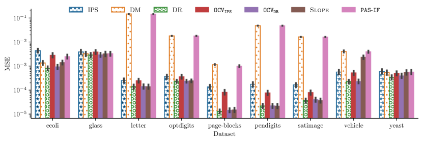
Figure 1: MSE of our estimator selection methods, $\tt OCV_{\textsc{IPS}}$ and $\tt OCV_{\textsc{DR}}$, compared against two other estimator selection baselines, Slope and $\tt PAS\mathchar 45\relax IF$. The methods select the best estimator out of IPS, DM, and DR. We report $95\%$ confidence intervals for all results.

Cross-validation with DR performs well even when DR performs poorly

One may think that $\tt OCV_{\textsc{DR}}$ performs well in Figure 1 because the DR is also the best estimator (Dudik et al., , 2014). To disprove this, we change the temperature of the target policy to $\beta_{1}=-10$ and report the results in Figure 2. In this case, the DR is no longer the best estimator, yet $\tt OCV_{\textsc{DR}}$ performs well. Both of our methods outperform Slope and $\tt PAS\mathchar 45\relax IF$ again. We also see that Slope performs worse in this setup. Since both IPS and DR are unbiased, their confidence intervals often overlap. Hence, Slope mostly chooses DR regardless of its performance.

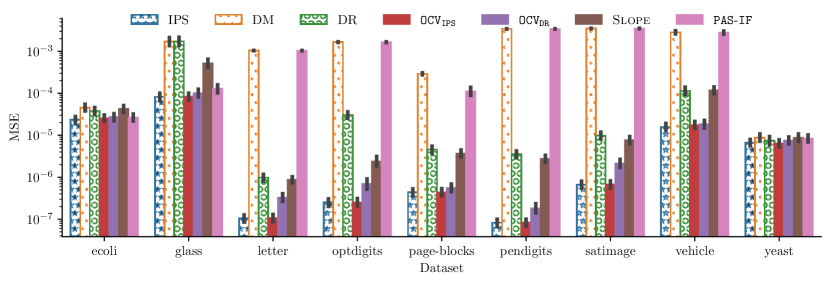
Figure 2: MSE of the estimator selection methods for temperatures $\beta_{0}=1$ and $\beta_{1}=-10$.

Cross-validation is computationally efficient

To split the dataset, $\tt PAS\mathchar 45\relax IF$ has to solve a complex optimization problem using a neural network. This is computationally costly and sensitive to tuning. We tuned the neural network architecture and loss function to improve the convergence and stability of $\tt PAS\mathchar 45\relax IF$. We also run it on a dedicated GPU and provide more details in Section A.2. Despite this, our methods are $100$ times less computationally costly than $\tt PAS\mathchar 45\relax IF$ (Table 1).

Method	$\tt OCV_{\textsc{IPS}}$	$\tt OCV_{\textsc{DR}}$	Slope	$\tt PAS\mathchar 45\relax IF$
Time	0.06s	0.13s	0.005s	13.91s

Table 1: Average computational cost of a single policy evaluation from Figure 1 when doing $K=10$ training/validation splits with $\tt OCV_{\textsc{DR}}$, $\tt OCV_{\textsc{IPS}}$, and $\tt PAS\mathchar 45\relax IF$. Computed on AMD Ryzen 9 8945HS and NVIDIA GeForce RTX 4070 Laptop.

6.2 Hyper-parameter tuning

We also evaluate $\tt OCV$ on the hyper-parameter tuning of seven estimators from Section 3. We present them next. TruncatedIPS (Ionides, , 2008) is parameterized by a clipping constant $M$ that clips higher propensity weights than $M$. The authors propose setting it to $M=\sqrt{N}$. Switch-DR (Wang et al., , 2017) has a threshold parameter $\tau$ that switches to DM if the propensity weights are too high and uses DR otherwise. The authors propose their own tuning strategy by pessimistically bounding the estimator’s bias (Wang et al., , 2017). CAB (Su et al., , 2019) has a parameter $M$ that adaptively blends DM and IPS. The authors do not propose any tuning method. DRos and DRps (Su et al., 2020a, ) have a parameter $\lambda$ that regularizes propensity weights to decrease DR’s variance. The authors also propose an improved tuning strategy similar to that of Switch-DR. IPS-$\lambda$ (Metelli et al., , 2021) has a parameter $\lambda$ that regularizes propensity weights while keeping the estimates differentiable, which is useful for off-policy learning. The authors propose a differentiable tuning objective to get optimal $\lambda$. GroupIPS (Peng et al., , 2023) has multiple tuning parameters, such as the number of clusters $M$, the reward model class to identify similar actions, and the clustering algorithm. The authors propose choosing $M$ by Slope. We describe the estimators, their original tuning procedures, and hyper-parameter grids used in this experiment in Section A.1.

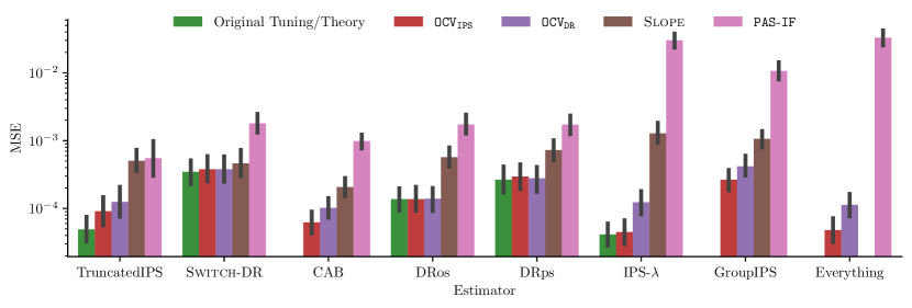
Figure 3: MSE of our methods applied to hyper-parameter tuning of various estimators. We compare them to Slope, $\tt PAS\mathchar 45\relax IF$, and originally proposed approaches by the authors. Everything refers to the joint estimator selection and hyper-parameter tuning.

All methods are evaluated in $90$ conditions: $9$ UCI ML Repository datasets (Bache and Lichman, , 2013), two target policies $\beta_{1}\in\{-10,10\}$, and five logging policies $\beta_{0}\in\{-3,-1,0,1,3\}$. This covers a wide range of scenarios: logging and target policies can be close or different, their values can be high or low, and dataset sizes vary from small ($107$) to larger ($10\,000$). Each condition is repeated $5$ times, and we report the MSE over all runs and conditions in Figure 3. We observe that theory-suggested hyper-parameter values generally perform the best if they exist. Surprisingly, $\tt OCV$ often matches their performance while also being a general solution that applies to any estimator. It typically outperforms Slope and $\tt PAS\mathchar 45\relax IF$.

We also consider the problem of joint estimator selection and hyper-parameter tuning. We evaluate $\tt OCV_{\textsc{DR}}$, $\tt OCV_{\textsc{IPS}}$, and $\tt PAS\mathchar 45\relax IF$ on this task and report our results as Everything in Figure 3. We do not evaluate Slope because the correct order of the estimators is unclear. We observe that both of our estimators perform well and have an order of magnitude lower MSE than $\tt PAS\mathchar 45\relax IF$. This shows that $\tt OCV$ is a reliable and practical method for joint estimator selection and hyper-parameter tuning.

7 Conclusion

We propose a data-driven estimator selection and hyper-parameter tuning procedure for off-policy evaluation that uses cross-validation, bridging an important gap between off-policy evaluation and supervised learning. Estimator selection in off-policy evaluation has been mostly theory-driven. In contrast, in supervised learning, cross-validation is preferred despite limited theoretical support. The main issue of an unknown policy value can be overcome by using an unbiased estimator on a held-out validation set. This is similar to cross-validation in supervised learning, where we only have samples from an unknown distribution. We test our method extensively on nine real-world datasets, and both estimator selection and hyper-parameter tuning tasks. The method is widely applicable, simple to implement, and easy to understand since it only relies on principal techniques from supervised learning that are well-known and loved by practitioners. More than that, it outperforms state-of-the-art methods.

One natural future direction is an extension to off-policy learning. The main challenge is that the tuned hyper-parameters have to work well for any policy instead of a single target policy. At the same time, naive tuning of some worst-case empirical risk could lead to too conservative choices. Another potential direction is an extension to reinforcement learning.

Appendix A Implementation details

Datasets

All datasets are publicly available online. In particular, we use the OpenML dataset repository (Vanschoren et al., , 2014). If there are multiple datasets with the same name, we always use version v.1. The following table summarizes dataset statistics.

Dataset	ecoli	glass	letter	optdigits	page-blocks	pendigits	satimage	vehicle	yeast
Classes	8	6	26	10	5	10	6	4	10
Features	7	9	16	64	10	16	36	18	8
Sample size	336	214	20000	5620	5473	10992	6435	846	1484

A.1 Estimators tuned in the experiments

To simplify the notation in this section, we define propensity weights $\displaystyle w(x_{i},a_{i})=\frac{\pi(a_{i}\mid x_{i})}{\pi_{0}(a_{i}\mid x_{i})}$.

TruncatedIPS

The truncated inverse propensity scores estimator (Ionides, , 2008) introduces a clipping constant $M>0$ to the IPS weights

$$\hat{V}_{\text{TruncatedIPS}}(\pi;\mathcal{D},M)=\frac{1}{N}\sum_{i=1}^{N}\min\left\{M,w(x_{i},a_{i})\right\}r_{i}\,.$$ (9)

This allows trading off bias and variance. When $M=\infty$, TIPS reduces to IPS. When $M=0$, the estimator returns 0 for any policy $\pi$. The theory suggests to set $M=\mathcal{O}(\sqrt{N})$ (Ionides, , 2008). In our experiments, we search for $M$ on the hyperparameter grid of 30 geometrically spaced values. The smallest and largest $\tau$ values in the grid are $w_{0.05}$ and $w_{0.95}$, denoting the 0.05 and 0.95 quantiles of the propensity weights. We also include the theory-suggested value in the grid.

Switch-DR

The switch doubly-robust estimator (Wang et al., , 2017) introduces a threshold parameter $\tau$ to ignore residuals of $\hat{f}(x_{i},a_{i})$ that have too large propensity weights

$$\hat{V}_{\textsc{Switch-DR}}(\pi;\mathcal{D},\tau)=\frac{1}{N}\sum_{i=1}^{N}\mathds{1}\!\left\{w(x_{i},a_{i})\leq\tau\right\}w(x_{i},a_{i})(r_{i}-\hat{f}(x_{i},a_{i}))+\hat{V}_{\textsc{DM}}(\pi;\mathcal{D})\,.$$ (10)

When $\tau=0$, Switch-DR becomes DM (2) whereas $\tau=\infty$ makes it DR (3). The authors propose a tuning procedure where they conservatively upper bound bias of DM to the largest possible value for every data point. This is to preserve the minimax optimality of Switch-DR with using estimated $\hat{\tau}$ as the threshold would only be activated if the propensity weights suffered even larger variance

$$\hat{\tau}=\operatorname*{arg\,min\,}_{\tau}\mathrm{var}\left[\hat{V}_{\textsc{Switch-DR}}(\pi;\mathcal{D},\tau)\right]+\text{Bias}_{\tau}^{2}$$ (11)

$$\text{Bias}_{\tau}^{2}=\left[\frac{1}{N}\sum_{i=1}^{N}\mathbb{E}_{\pi}\left[R_{\text{max}}\mathds{1}\!\left\{w(x_{i},a_{i})>\tau\right\}\mid x_{i}\right]\right]^{2}\,,$$ (12)

where the authors assume we know maximal reward value $0\leq r(x,a)\leq R_{\text{max}}$, which in our experiments is set at $R_{\text{max}}=1$. We define the grid in our experiments similarly to that of TruncatedIPS, where the grid has 30 geometrically spaced values. The smallest and largest $\tau$ values in the grid are $w_{0.05}$ and $w_{0.95}$. The authors originally proposed a grid of 21 values where the smallest and the largest values are the minimum and maximum of the propensity weights. Still, we decided on this grid as we did not observe negative changes in the estimator’s performance, and we want to keep the grid consistent with the subsequent estimators.

CAB

The continuous adaptive blending estimator (Su et al., , 2019) weights IPS and DM parts based on propensity weights, where DM is preferred when the propensity weights are large and vice versa

$$\hat{V}_{\textsc{CAB}}(\pi;\mathcal{D},M)=\frac{1}{N}\sum_{i=1}^{N}\sum_{a\in\mathcal{A}}\pi(a\mid x_{i})\alpha_{i}(a)\hat{f}(x_{i},a)+\frac{1}{N}\sum_{i=1}^{N}w(x_{i},a_{i})\beta_{i}r_{i}\,,$$ (13)

$$\alpha_{i}(a)=1-\min\left\{Mw(x_{i},a)^{-1},1\right\}\,,\;\beta_{i}=\min\left\{Mw(x_{i},a_{i})^{-1},1\right\}\,.$$ (14)

The estimator reduces to DM when $M=0$ and to IPS when $M=\infty$. The advantage is that this estimator is sub-differentiable, which allows it to be used for policy learning. The authors do not propose any tuning procedure. In our experiments, we search for $M$ on the hyperparameter grid of 30 geometrically spaced values with the smallest and largest $M$ values in the grid $w_{0.05}$ and $w_{0.95}$.

DRos, DRps

The doubly-robust estimators with optimistic and pessimistic shrinkages (Su et al., 2020a, ) are the estimators that shrink the propensity weights to minimize a bound on the mean squared error

$$\hat{V}_{\textsc{DRs}}(\pi;\mathcal{D},\lambda)=\frac{1}{N}\sum_{i=1}^{N}\hat{w}_{\lambda}(x_{i},a_{i})(r_{i}-\hat{f}(x_{i},a_{i}))+\hat{V}_{\textsc{DM}}(\pi;\mathcal{D})\,,$$ (15)

$$\hat{w}_{o,\lambda}(x,a)=\frac{\lambda}{w(x,a)^{2}+\lambda}w(x,a)\,,\;\hat{w}_{p,\lambda}(x,a)=\min\left\{\lambda,w(x,a)\right\}\,,$$ (16)

where $\hat{w}_{o,\lambda}$ and $\hat{w}_{p,\lambda}$ are the respective optimistic and pessimistic weight shrinking variants, and we refer to the estimators that use them as DRos and DRps. In both cases, the estimator reduces to DM when $\lambda=0$ and to DR when $\lambda=\infty$. The authors also propose a tuning procedure to estimate $\hat{\lambda}=\operatorname*{arg\,min\,}_{\lambda}\mathrm{var}\left[\hat{V}_{\textsc{DRs}}(\pi;\mathcal{D},\lambda)\right]+\text{Bias}_{\lambda}^{2}$ where they bound the bias as follows

$$\text{Bias}_{\lambda}^{2}=\left[\frac{1}{N}\sum_{i=1}^{N}(\hat{w}_{\lambda}(x_{i},a_{i})-w(x_{i},a_{i}))(r_{i}-\hat{f}(x_{i},a_{i})\right]^{2}.$$ (17)

According to the authors, our experiments define the hyper-parameter grid of 30 geometrically spaced values. For DRos, the smallest and largest $lambda$ values on the grid are $0.01\times(w_{0.05})^{2}$ and $100\times(w_{0.95})^{2}$ and for DRps, they are $w_{0.05}$ and $w_{0.95}$.

IPS-$\boldsymbol{\lambda}$

The subgaussian inverse propensity scores estimator (Metelli et al., , 2021) improves polynomial concentration of IPS (1) to subgaussian by correcting the propensity weights

$$\hat{V}_{\textsc{IPS-}\lambda}(\pi;\mathcal{D},\lambda)=\frac{1}{N}\sum_{i=1}^{N}\frac{w(x_{i},a_{i})}{1-\lambda+\lambda w(x_{i},a_{i})}r_{i}\,.$$ (18)

When $\lambda=0$, the estimator reduces to IPS, and when $\lambda=1$, the estimator returns 1 for any $\pi$. Note that this is the harmonic correction, while a more general definition uses propensity weights $\displaystyle w_{\lambda,s}(x,a)=\left((1-\lambda)w(x,a)^{s}+\lambda\right)^{\frac{1}{s}}$. The authors also propose a tuning procedure where they choose $\lambda$ by solving the following equation

$$\lambda^{2}\frac{1}{N}\sum_{i=1}^{N}w_{\lambda,\sqrt[4]{N}}(x_{i},a_{i})^{2}=\frac{2\log\frac{1}{\delta}}{3N}\,.$$ (19)

The equation uses a general definition of $w_{\lambda,s}$ where $s=\sqrt[4]{N}$ and can be solved by gradient descent. As this parameter has an analytic solution, the authors did not specify any hyper-parameter grid. We define the grid to be $(1+\exp(-x))^{-1}_{(h\in[-10,10])}$ where $(h\in[-10,10])$ are 30 linearly spaced values.

GroupIPS

The outcome-oriented action grouping IPS estimator (Peng et al., , 2023) has multiple parameters: the reward model class, the clustering algorithm, and the number of clusters. In GroupIPS, one first learns a reward model $\hat{f}(x,a)$ to estimate the mean reward. The reward model is then used to identify similar actions. The authors (Peng et al., , 2023), in their experiments, use a neural network for it. We simplify it in line with other baselines. We learn the same ridge regression model and use the estimated mean reward $\hat{f}(x,a)$ to group context-action pairs. More formally, a clustering algorithm $\mathcal{G}$ learns a mapping $g=\mathcal{G}(\mathcal{D},\hat{f},M)$ that assigns each context-action pair $(x,a)\in\mathcal{D}$ to a cluster $m\in M$ based on its estimated mean reward $\hat{f}(x,a)$. While the authors originally used K-means clustering, in our experiments, we use uniform binning as it is computationally more efficient. We split the reward space $[0,1]$ into $M$ equally spaced intervals and assign each context-action pair to the corresponding interval based on its estimated mean reward. Finally, IPS is used to reweight the policies based on the propensity weights of each cluster

$$\hat{V}_{\text{GroupIPS}}(\pi;\mathcal{D},M)=\frac{1}{N}\sum_{i=1}^{N}\frac{\pi(g(x_{i},a_{i})\mid x_{i})}{\pi_{0}(g(x_{i},a_{i})\mid x_{i})}r_{i}$$ (20)

where $\pi(m,x)=\sum_{a\in\mathcal{A}}\mathds{1}\!\left\{g((x,a)=m\right\}\pi(a\mid x)$ is a shorthand for the conditional probability of recommending any action mapped to cluster $m$ in context $x$. We still need to tune $M$, and the prior work (Peng et al., , 2023) uses Slope for it. In our experiments, we define the hyper-parameter grid for the number of clusters $M$ as $\left\{2,4,8,16,32\right\}$.

A.2 Estimator selection and hyper-parameter tuning

Variance estimation

Slope and $\tt OCV$ estimate the estimator’s variance as part of their algorithm. Slope derives the estimator’s confidence intervals from it, and $\tt OCV$ uses it to set the optimal training/validation ratio.

All estimators in Sections 2 and A.1 are averaging over $N$ observations $(x_{i},a_{i},r_{i})$ and we use this fact for variance estimation in line with other works (Wang et al., , 2017; Su et al., 2020b, ). We illustrate this on TruncatedIPS. Let $\hat{v}_{i}(M)=\min\left\{M,w(x_{i},a_{i})\right\}r_{i}$ be the value estimate of $\pi$ for a single observation $(x_{i},a_{i},r_{i})$ and averaging over it leads to $\bar{v}_{M}=\hat{V}_{\text{TruncatedIPS}}(\pi;\mathcal{D},M)=\frac{1}{N}\sum_{i=1}^{N}\hat{v}_{i}(M)$ . Since $x_{i}$ are i.i.d., the variance can be estimated as

$$\sigma^{2}_{M}\approx\frac{1}{N^{2}}\sum_{i=1}^{N}\left(\hat{v}_{i}(M)-\bar{v}_{M}\right)^{2}\,.$$ (21)

Using this technique in Slope, we get the 95% confidence intervals as $\left[\bar{v}_{M}-2\sigma_{M},\bar{v}_{M}+2\sigma_{M}\right]$. This is also valid estimate in our experiments since $r_{i}\in[0,1]$, all policies are constrained to the class defined in (8), which ensures $\pi_{0}$ has full support, hence $\hat{v}_{i}$ are bounded.

Slope

We use 95% confidence intervals according to the original work of Su et al., 2020b . In Section 6.1, we use the order of the estimators $\mathrm{var}\left[\hat{V}_{\textsc{IPS}}(\pi)\right]\geq\mathrm{var}\left[\hat{V}_{\textsc{DR}}(\pi)\right]\geq\mathrm{var}\left[\hat{V}_{\textsc{DM}}(\pi)\right]$. The order of the hyper-parameter values for seven estimators tuned in Section 6.2 is summarized in the following table.

Estimator	TruncatedIPS	Switch-DR	CAB	DRos	DRps	IPS-$\lambda$	GroupIPS
Variance order	$w_{0.05}\leq w_{0.95}$	$w_{0.05}\leq w_{0.95}$	$w_{0.05}\leq w_{0.95}$	$(w_{0.05})^{2}\leq(w_{0.95})^{2}$	$w_{0.05}\leq w_{0.95}$	$h_{-10}\geq h_{10}$	$M_{2}\leq M_{32}$

Except for IPS-$\lambda$, a hyper-parameter of a higher value results in a higher-variance estimator; hence, the algorithm starts with these.

PAS-IF

The tuning procedure of $\tt PAS\mathchar 45\relax IF$ uses a neural network to split the dataset and create surrogate policies. We modify the original code from the authors’ GitHub to speed up the execution and improve stability. We use the same architecture as the authors (Udagawa et al., , 2023), a 3-layer MLP with 100 neurons in each hidden layer and ReLU activation. We observed numerical instabilities on some of our datasets. Hence, we added a 20% dropout and batch normalization after each hidden layer. The final layer has sigmoid activation. We use Adam as its optimizer. We use a batch size of 1000, whereas the authors used 2000. The loss function consists of two terms, $\mathcal{L}=\mathcal{L}_{d}+\alpha\mathcal{L}_{r}$, where $\mathcal{L}_{d}$ forces the model to output the propensity weights of surrogate policies that match the original $(w(x_{i},a_{i}))_{i\in[N]}$, and $\mathcal{L}_{r}$ forces the model to split the dataset using 80/20 training/validation ratio. The authors iteratively increase the coefficient $\alpha\in[0.1,1,10,100,1000]$ until the resulting training/validation ratio is 80/20 $\pm$ 2. This results in a lot of computation overhead; hence, we dynamically set $\alpha=0$ if the ratio is within 80/20 $\pm$ 2 and $\alpha=1000$ otherwise. Finally, if the logging and target policies substantially differ, the propensity weights $w(x,a)$ are too large, and the original loss function becomes numerically unstable. Hence, we clip the target weights $\min\left\{w(x,a),10^{7}\right\}$. The clipping is loose enough not to alter the algorithm’s performance but enough to keep the loss numerically stable. Finally, we run $\tt PAS\mathchar 45\relax IF$ for 5000 epochs as proposed by the authors, but we added early stopping at five epochs (the tolerance set at $10^{-3}$), and the algorithm usually converges within 100 epochs.

Appendix B Additional experiments

In these experiments, we perform ablation on the individual components of our method to empirically support our decisions, namely theory-driven training/validation split ratio and the one standard error rule. We also ablate the number of repeated splits $K$ and show that a higher number improves the downstream performance, but we observe diminishing returns as the results observed in repeated splits are correlated. We also discuss the importance of choosing an unbiased validation estimator, and we empirically show DM as a validation estimator performs poorly.

Our improvements make standard cross-validation more stable

Our method has two additional components to reduce the variance of validation error: the training/validation split ratio and one standard error rule. We discuss them in Sections 5.1 and 5.2. We ablate our method, gradually adding these components. We use the same setup as in Figure 1, average the results over all datasets, and report them in Figure 4. We start with standard 10-fold cross-validation where different validation splits do not overlap; hence, the training/validation ratio is set at 90/10. We also choose the estimator with the lowest mean squared error, not the lowest upper bound. In Figure 4, we call this method A: $\tt OCV_{\textsc{DR}}$ 90/10 split ratio. As a next step, we change the selection criterion from the mean loss to the upper bound on mean loss (B: A + one SE rule). We observe dramatic improvements, making the method more robust so it does not choose the worst estimator. Then, instead, we try our adaptive split ratio as suggested in Section 5.1 and see this yields even bigger improvements (C: A + theory split ratio). We then combine these two improvements together (D: B + C). This corresponds to the method we use in all other experiments. We see the one standard error rule does not give any additional improvements anymore, as our theory-driven training/validation ratio probably results in similarly-sized confidence intervals on the estimator’s MSE. Additionally, as the theory-suggested ratio is not dependent on $K$ number of splits, we also change it to $K=100$, showing this gives additional marginal improvements (E: D + 100 K training/test splits).

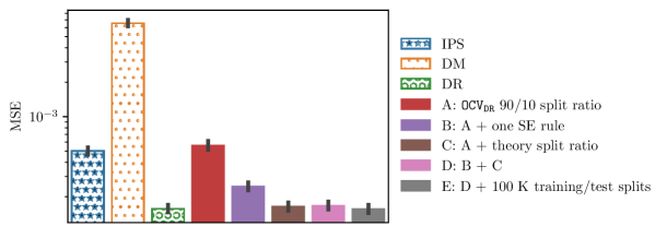
Figure 4: Ablation on proposed improvements from Sections 5.1 and 5.2 with $\tt OCV_{\textsc{DR}}$. This shows that both improvements individually help reduce the variance of estimation errors. However, when combined, the theory split ratio makes the one standard error rule insignificant.

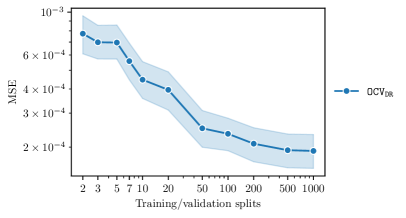
Figure 5: Ablation of the number of repeated training/validation splits with $\tt OCV_{\textsc{DR}}$ on the vehicle dataset averaged over 500 runs. This shows us diminishing improvements as we increase the number of splits.

We show in more detail in Figure 5 how the CV performance improves with the increasing number of training/validation splits. As expected, there are diminishing returns with an increasing number of splits. As the splits are correlated, there is an error limit towards which our method converges with increasing $K$.

The validation estimator used in cross-validation has to be unbiased

In Section 5, we constrain the validation estimator $\tilde{V}$ to the class of unbiased estimators, such as IPS (1), DR (3) or others we did not mention, such as SNIPS (Swaminathan and Joachims, , 2015). In Lemma 1, bias term $b$ in the CV objective contains only bias of $\hat{V}$. This no longer holds if $\tilde{V}$ is biased, as $\mathbb{E}\left[\tilde{V}_{k}\right]\neq V$. Our optimization objective would be shifted to prefer the estimators biased in the same direction. This might be the case of poor $\tt PAS\mathchar 45\relax IF$’s performance as its estimate on the validation set is not unbiased. We demonstrate this behavior on the same experimental setup as in Figure 1. We use DM as $\tilde{V}$ and report the results in Figure 6 averaged over 100 independent runs. The estimator selection procedure of $\tt OCV_{\textsc{DM}}$ is biased in the same direction as the DM estimator, and the procedure selects it even though it performs poorly. To compare it with $\tt OCV_{\textsc{DR}}$, we see DR performs poorly in Figure 2, especially on the glass dataset. However, $\tt OCV_{\textsc{DR}}$ still performs.

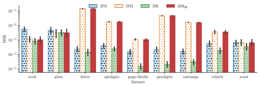
Figure 6: MSE of cross-validation, when using DM as a validation estimator. As DM is biased, it systematically chooses an estimator that is biased in the same direction: DM itself.

References

- Akaike, (1998) Akaike, H. (1998). Information Theory and an Extension of the Maximum Likelihood Principle. In Parzen, E., Tanabe, K., and Kitagawa, G., editors, Selected Papers of Hirotugu Akaike, pages 199–213. Springer New York, New York, NY. Series Title: Springer Series in Statistics.
- Aouali et al., (2023) Aouali, I., Brunel, V.-E., Rohde, D., and Korba, A. (2023). Exponential Smoothing for Off-Policy Learning. In Proceedings of the 40th International Conference on Machine Learning, pages 984–1017. PMLR. ISSN: 2640-3498.
- Bache and Lichman, (2013) Bache, K. and Lichman, M. (2013). UCI Machine Learning Repository.
- Bishop, (2006) Bishop, C. M. (2006). Pattern recognition and machine learning. Information science and statistics. Springer, New York.
- Buckman et al., (2020) Buckman, J., Gelada, C., and Bellemare, M. G. (2020). The Importance of Pessimism in Fixed-Dataset Policy Optimization. In International Conference on Learning Representations.
- Cief et al., (2024) Cief, M., Golebiowski, J., Schmidt, P., Abedjan, Z., and Bekasov, A. (2024). Learning Action Embeddings for Off-Policy Evaluation. In Goharian, N., Tonellotto, N., He, Y., Lipani, A., McDonald, G., Macdonald, C., and Ounis, I., editors, Advances in Information Retrieval, pages 108–122, Cham. Springer Nature Switzerland.
- Devroye et al., (1996) Devroye, L., Györfi, L., and Lugosi, G. (1996). A Probabilistic Theory of Pattern Recognition, volume 31 of Stochastic Modelling and Applied Probability. Springer New York, New York, NY.
- Dudik et al., (2014) Dudik, M., Erhan, D., Langford, J., and Li, L. (2014). Doubly Robust Policy Evaluation and Optimization. Statistical Science, 29(4):485–511.
- Farajtabar et al., (2018) Farajtabar, M., Chow, Y., and Ghavamzadeh, M. (2018). More Robust Doubly Robust Off-policy Evaluation. In Proceedings of the 35th International Conference on Machine Learning, pages 1447–1456. PMLR. ISSN: 2640-3498.
- Hastie et al., (2009) Hastie, T., Tibshirani, R., and Friedman, J. (2009). The Elements of Statistical Learning. Springer Series in Statistics. Springer New York, New York, NY.
- Hauskrecht and Fraser, (2000) Hauskrecht, M. and Fraser, H. (2000). Planning treatment of ischemic heart disease with partially observable Markov decision processes. Artificial Intelligence in Medicine, 18(3):221–244.
- Ionides, (2008) Ionides, E. L. (2008). Truncated Importance Sampling. Journal of Computational and Graphical Statistics, 17(2):295–311.
- Kallus and Zhou, (2018) Kallus, N. and Zhou, A. (2018). Policy Evaluation and Optimization with Continuous Treatments. In Proceedings of the Twenty-First International Conference on Artificial Intelligence and Statistics, pages 1243–1251. PMLR. ISSN: 2640-3498.
- Langford et al., (2008) Langford, J., Strehl, A., and Wortman, J. (2008). Exploration scavenging. In Proceedings of the 25th international conference on Machine learning, ICML ’08, pages 528–535, New York, NY, USA. Association for Computing Machinery.
- Lee et al., (2022) Lee, J., Tucker, G., Nachum, O., and Dai, B. (2022). Model Selection in Batch Policy Optimization. In Proceedings of the 39th International Conference on Machine Learning, pages 12542–12569. PMLR. ISSN: 2640-3498.
- Lepski and Spokoiny, (1997) Lepski, O. V. and Spokoiny, V. G. (1997). Optimal pointwise adaptive methods in nonparametric estimation. The Annals of Statistics, 25(6):2512–2546. Publisher: Institute of Mathematical Statistics.
- Li et al., (2010) Li, L., Chu, W., Langford, J., and Schapire, R. E. (2010). A contextual-bandit approach to personalized news article recommendation. In Proceedings of the 19th international conference on World wide web, WWW ’10, pages 661–670, New York, NY, USA. Association for Computing Machinery.
- Metelli et al., (2021) Metelli, A. M., Russo, A., and Restelli, M. (2021). Subgaussian and Differentiable Importance Sampling for Off-Policy Evaluation and Learning. In Advances in Neural Information Processing Systems, volume 34, pages 8119–8132. Curran Associates, Inc.
- Nie et al., (2022) Nie, A., Flet-Berliac, Y., Jordan, D., Steenbergen, W., and Brunskill, E. (2022). Data-Efficient Pipeline for Offline Reinforcement Learning with Limited Data. Advances in Neural Information Processing Systems, 35:14810–14823.
- Peng et al., (2023) Peng, J., Zou, H., Liu, J., Li, S., Jiang, Y., Pei, J., and Cui, P. (2023). Offline Policy Evaluation in Large Action Spaces via Outcome-Oriented Action Grouping. In Proceedings of the ACM Web Conference 2023, WWW ’23, pages 1220–1230, New York, NY, USA. Association for Computing Machinery.
- Robins et al., (1994) Robins, J. M., Rotnitzky, A., and Zhao, L. P. (1994). Estimation of Regression Coefficients When Some Regressors are not Always Observed. Journal of the American Statistical Association, 89(427):846–866. Publisher: Taylor & Francis _eprint: https://doi.org/10.1080/01621459.1994.10476818.
- Sachdeva et al., (2023) Sachdeva, N., Wang, L., Liang, D., Kallus, N., and McAuley, J. (2023). Off-Policy Evaluation for Large Action Spaces via Policy Convolution. arXiv:2310.15433 [cs].
- Saito and Joachims, (2022) Saito, Y. and Joachims, T. (2022). Off-Policy Evaluation for Large Action Spaces via Embeddings. In Proceedings of the 39th International Conference on Machine Learning, pages 19089–19122. PMLR. ISSN: 2640-3498.
- Saito and Nomura, (2024) Saito, Y. and Nomura, M. (2024). Hyperparameter Optimization Can Even be Harmful in Off-Policy Learning and How to Deal with It. arXiv:2404.15084 [cs].
- Saito et al., (2023) Saito, Y., Ren, Q., and Joachims, T. (2023). Off-Policy Evaluation for Large Action Spaces via Conjunct Effect Modeling. In Proceedings of the 40th International Conference on Machine Learning, pages 29734–29759. PMLR. ISSN: 2640-3498.
- Saito et al., (2021) Saito, Y., Udagawa, T., Kiyohara, H., Mogi, K., Narita, Y., and Tateno, K. (2021). Evaluating the Robustness of Off-Policy Evaluation. In Proceedings of the 15th ACM Conference on Recommender Systems, RecSys ’21, pages 114–123, New York, NY, USA. Association for Computing Machinery.
- Schwarz, (1978) Schwarz, G. (1978). Estimating the Dimension of a Model. The Annals of Statistics, 6(2).
- Silver et al., (2013) Silver, D., Newnham, L., Barker, D., Weller, S., and McFall, J. (2013). Concurrent Reinforcement Learning from Customer Interactions. In Proceedings of the 30th International Conference on Machine Learning, pages 924–932. PMLR. ISSN: 1938-7228.
- Stoica and Selen, (2004) Stoica, P. and Selen, Y. (2004). Model-order selection. IEEE Signal Processing Magazine, 21(4):36–47.
- Stone, (1974) Stone, M. (1974). Cross-Validatory Choice and Assessment of Statistical Predictions. Journal of the Royal Statistical Society Series B: Statistical Methodology, 36(2):111–133.
- (31) Su, Y., Dimakopoulou, M., Krishnamurthy, A., and Dudik, M. (2020a). Doubly robust off-policy evaluation with shrinkage. In Proceedings of the 37th International Conference on Machine Learning, pages 9167–9176. PMLR. ISSN: 2640-3498.
- (32) Su, Y., Srinath, P., and Krishnamurthy, A. (2020b). Adaptive Estimator Selection for Off-Policy Evaluation. In Proceedings of the 37th International Conference on Machine Learning, pages 9196–9205. PMLR. ISSN: 2640-3498.
- Su et al., (2019) Su, Y., Wang, L., Santacatterina, M., and Joachims, T. (2019). CAB: Continuous Adaptive Blending for Policy Evaluation and Learning. In Proceedings of the 36th International Conference on Machine Learning, pages 6005–6014. PMLR. ISSN: 2640-3498.
- Swaminathan and Joachims, (2015) Swaminathan, A. and Joachims, T. (2015). The Self-Normalized Estimator for Counterfactual Learning. In Advances in Neural Information Processing Systems, volume 28. Curran Associates, Inc.
- Udagawa et al., (2023) Udagawa, T., Kiyohara, H., Narita, Y., Saito, Y., and Tateno, K. (2023). Policy-Adaptive Estimator Selection for Off-Policy Evaluation. In Proceedings of the AAAI Conference on Artificial Intelligence, volume 37, pages 10025–10033.
- Vanschoren et al., (2014) Vanschoren, J., van Rijn, J. N., Bischl, B., and Torgo, L. (2014). OpenML: networked science in machine learning. ACM SIGKDD Explorations Newsletter, 15(2):49–60.
- Varma and Simon, (2006) Varma, S. and Simon, R. (2006). Bias in error estimation when using cross-validation for model selection. BMC Bioinformatics, 7(1):91.
- Voloshin et al., (2021) Voloshin, C., Le, H., Jiang, N., and Yue, Y. (2021). Empirical Study of Off-Policy Policy Evaluation for Reinforcement Learning. In Proceedings of the Neural Information Processing Systems Track on Datasets and Benchmarks, volume 1.
- Wang et al., (2017) Wang, Y.-X., Agarwal, A., and Dudik, M. (2017). Optimal and Adaptive Off-policy Evaluation in Contextual Bandits. In Proceedings of the 34th International Conference on Machine Learning, pages 3589–3597. PMLR. ISSN: 2640-3498.
- Wilson et al., (2017) Wilson, J. T., Moriconi, R., Hutter, F., and Deisenroth, M. P. (2017). The reparameterization trick for acquisition functions. arXiv:1712.00424 [cs, math, stat].
- Yao et al., (2007) Yao, Y., Rosasco, L., and Caponnetto, A. (2007). On Early Stopping in Gradient Descent Learning. Constructive Approximation, 26(2):289–315.