11email: {xingjianwang,chaili,cjm}@zju.edu.cn
Frequency-Domain Refinement with
Multiscale Diffusion for Super Resolution
Abstract
The performance of single image super-resolution depends heavily on how to generate and complement high-frequency details to low-resolution images. Recently, diffusion-based models exhibit great potential in generating high-quality images for super-resolution tasks. However, existing models encounter difficulties in directly predicting high-frequency information of wide bandwidth by solely utilizing the high-resolution ground truth as the target for all sampling timesteps. To tackle this problem and achieve higher-quality super-resolution, we propose a novel Frequency Domain-guided multiscale Diffusion model (FDDiff), which decomposes the high-frequency information complementing process into finer-grained steps. In particular, a wavelet packet-based frequency complement chain is developed to provide multiscale intermediate targets with increasing bandwidth for reverse diffusion process. Then FDDiff guides reverse diffusion process to progressively complement the missing high-frequency details over timesteps. Moreover, we design a multiscale frequency refinement network to predict the required high-frequency components at multiple scales within one unified network. Comprehensive evaluations on popular benchmarks are conducted, and demonstrate that FDDiff outperforms prior generative methods with higher-fidelity super-resolution results.
Keywords:
Frequency-Domain Refinement Multiscale Diffusion1 Introduction
Super-resolution (SR) for single image is a crucial task and has attracted constant research interests, which plays a vital role in enhancing the quality of low-resolution (LR) images for various downstream tasks. From a frequency-domain perspective, the natural or artificial degradation process causing LR images can be regarded as an extensive low-pass filtering on the corresponding high-resolution (HR) images, resulting in a significant loss of high-frequency details. Hence the main difficulty of reconstructing high-quality HR images lies in the restoration of the missing high-frequency information.
Recently, with the continuous innovation of deep learning techniques, there has witnessed various super-resolution methods. These methods can be split into two categories, namely regression-based methods and generative methods. Among them, regression-based methods[5, 24, 3] directly learn the LR-to-HR mapping. Although achieving relatively small pixel-wise errors, regression-based methods suffer from low perceptual quality with insufficient high-frequency details. Instead, generative methods[20, 42, 41, 47, 25, 23, 9, 21, 36, 7, 29] have seen success in generating realistic details, which leverage the prior distribution learned from training dataset for super-resolution.
However, they also have various limitations. For instance, GAN-based SR methods[20, 42, 41, 47] are prone to unstable training and mode collapse, while Normalizing Flow-based[25, 23] and VAE-based[9] SR methods suffer from less visually pleasing SR results. As a recent member of generative methods, diffusion-based SR methods[21, 36, 7, 29] have made encouraging progress in generating high-quality SR images.
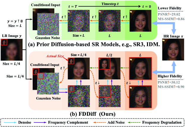
While there are diverse interpretations of super-resolution, the frequency-domain perspective of this paper on super-resolution involves complementing the missing high-frequency information to LR images. Existing diffusion-based SR methods[21, 36, 7, 29] mainly set the HR ground truth as the sole target throughout the whole reverse diffusion process without any intermediate targets or guidance. As a result, these methods have great difficulties to directly predict high-frequency information within a relatively wide bandwidth all at once, especially for large upscaling factors. As illustrated in DDIM[38], the diffusion forward process can be a non-Markovian process as long as the conditional distribution of the latent variable at time conditioned on its initial state remains the same with the one in DDPM[12]. Therefore, it is recommended to construct a non-Markovian forward process to provide prior frequency-domain guidance for the reverse diffusion SR process.
To address this problem, we propose a novel Frequency Domain-guided multiscale Diffusion model (FDDiff) to progressively complement the missing high-frequency components in LR images. Avoiding the difficulties of the direct transition from a simple Gaussian distribution to the complex HR image distribution in prior works[21, 36, 7, 29], we propose a wavelet packet-based frequency complement chain to additionally introduce easily accessible distributions to the diffusion reverse process. These intermediate distributions can be regard as temporally varying intermediate targets with progressively refined high-frequency information and hierachical scales. Based on the frequency complement chain, the corresponding multiscale frequency refinement diffusion is proposed to progressively predict the missing high-frequency information within a small local bandwidth step by steps, conditioned on LR images. Besides, a multiscale frequency refinement network with soft parameter-sharing is designed to handle latent variables of multiple sizes in multiscale diffusion process simultaneously within one network.
We evaluate FDDiff on various super-resolution tasks from face images[17, 16] to general images[1, 27, 6, 14]. Experimental results demonstrate that FDDiff outperforms other state-of-the-art generative methods, achieving high super-resolution quality both for regression-oriented and perception-oriented metrics.
2 Related Work
Diffusion Models for Super-Resolution With the rapid development of diffusion probabilistic models[12, 30, 38, 8], diffusion-based methods have exhibited impressive high SR quality. Adapting conditional diffusion model for super-resolution, SR3[36] and SRDiff[21] both iteratively denoised and transformed the latent variable sampling from simple Gaussian distribution to the HR image space with complex distributions, conditioned on LR input image. Based on SR3 and SRDiff, IDM[7] exploited implicit neural representation to learn SR with continuous upscaling ratios. Inspired by WaveDiff[33], DiWa[29] further denoised in Wavelet domain for faster sampling. However, they treat the super-resolution process merely as a denoising process with the straightforward application of conditional diffusion, and unavoidably encountered the difficulty to transform the simple Gaussian distribution into the complex distribution of HR images. Besides, taking the HR ground truth as the sole target for all timesteps incurs additional computational and memory cost, since the sizes of noised images in diffusion process remain the same as the input images. Instead, we introduce the temporally varying intermediate targets with hierachical scales to diffusion process, and guide the diffusion model to progressively restore the missing high-frequency information for LR images.
Super-Resoltuion in Frequency Domain Nowadays, conducting super-resolution tasks in wavelet-based frequency domain has attracted growing attention, and Wavelet Transform can benefit many applications in computer vision field. Several wavelet-based super-resolution works have been proposed, including Wavelet-SRNet[13], SRCliqueNet[48], and FSR[22]. Among them, Wavelet-SRNet[13] ultilized convolutional network to complement the wavelet high-frequency coefficients for LR images, while SRCliqueNet[48] and FSR[22] focused on design elaborate network to extract superior features fused from the four sub-bands of wavelet transform. However, as regression-based models, they are limited to achieve high perceptual quality due to the absence of randomness guidance inherent in generative models. Moreover, they merely employ wavelet to decompose images into four sub-bands and thus lack sufficiently detailed partitioning in frequency domain. Observed that Wavelet Packet-based Transform (WPT) has much more fine-grained frequency partition than Wavelet Transform [19], we exploit WPT to transition HR images into states with different frequency components, and incorporate the progressive frequency refinement process into diffusion process for higher SR quality.
3 Method
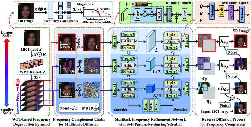
In this section, we describe our proposed FDDiff in detail. The overall architecture is illustrated in Fig. 2, while the training and inference algorithms are presented in Alg. 1 and Alg. 2 respectively.
3.1 Frequency Complement Chain
We design a high-frequency complement chain based on wavelet packet. Firstly, HR images are transitioned into sub-images of varying bandwidths. Then these sub-images are assigned to different timesteps through non-linear interpolation to provide high-frequency targets. Hence, diffusion model is guided to predict the missing high-frequency details within a small local bandwidth step by step.
Frequency Component Extraction To design a frequency complement chain, we first extracted frequency components of different bandwidths from images. Let be a given HR-LR image pair, where represents the expected high-resolution output images, represents low-resolution images, and denotes upscaling factor. Firstly, is iteratively convolved with the basis vectors of Wavelet Packet Transform (WPT) to be projected onto frequency domain at increasing stage , resulting in sub-image with more fine-grained frequency components along channel dimension. To be specific, given pre-stage sub-image , which utilizes a set of four fixed and even-sized convolution kernels with stride to divide the frequency bands of the image into four parts, i.e., low-frequency part by , horizontal high-frequency part by , vertical high-frequency part by , and diagonal high-frequency part by respectively. Haar wavelet kernels are selected as in this paper. As a result, the obtained sub-image have double downsampling scale and frequency components of narrower bandwidth compared to Such a quad-tree subband decomposition process can be defined as follows,
| (1) |
where denotes decomposition operation, and denotes concatenation operation along channel dimension. The reverse process of can be written as,
| (2) |
where and . denotes PixelShuffle[37] with upsampling factor. is the set of four fixed inverse kernels.
Multiscale Frequency Degradation Pyramid Based on the obtained sub-image by -times decomposition, we first build a multiscale degradation pyramid with cascaded upscaling. The channels of are split into parts of different frequency coefficients and sorted by their frequency, resulting in with frequency descending along the index. Among them, denotes the low-frequency part of , while the remaining ones are our intermediate targets. We define the low-pass operation to filter out high-frequency components conditioned on the given and , where and both are given frequency indexes from the set of integers . equals to when , otherwise it equals to zero. Then the -state multiscale sub-image degradation pyramid for is defined as follows,
| (3) |
where represents the ceiling function and . In this way, the pyramid degrades at st state to LR image at -th state.
Furthermore, the aforementioned states of should be assigned to timesteps. Since the low-frequency components with lower retaining larger energy are harder to be restored, it is suggested to lead the diffusion model to sample more timesteps for lower index . We therefore design the timestep assignment schedule based on power function, which can be expressed as,
| (4) |
Then the frequency degradation pyramid over timesteps can be derived from the sub-image pyramid as follows,
| (5) |
where the key timestep corresponding to state transition from to is set to . As for the boundary case, while , . Although the LR degradation of remains unknown, the frequency components of are encompassed within the low-frequency part of . Hence, the proposed chain first convert the frequency bandwidth of to the same as , as shown in Eq. 5 while . It is worth noting that the undergoes scale changing from to for those , while . As a result, of all timesteps forms a multiscale pyramid instead of a fixed-size chain, which will effectively reduce the memory and computation cost.
Accordingly, the frequency complement chain from to is given by the reverse process of this frequency degradation pyramid, where the missing high-frequency component , is provided as additional targets for diffusion model.
3.2 Multiscale Frequency Refinement Diffusion
Under the guidance of frequency complement chain, the non-Markovian diffusion process with multiscale latent variables is proposed to generate the missing high-frequency details for LR images.
Forward Process Inspired by DDIM[38] and f-DM[8], we design a noised latent variable with whose conditional distribution conforming to the one defined in DDPM[12]. is directly sampled around by
| (6) |
where the noise hyperparameter defined in [12] follows the cosine schedule in [30]. and monotonically decreases to zero over time. Evidently, and . To meet the marginal distribution, the non-Markovian diffusion forward process is given by,
| (7) |
where and denotes the added Gaussian noise for every forward step. For smooth transition between timesteps of different scales, the downsampling operation with integer factor is added between the scale-changing timesteps. That is, equals to if and , otherwise equals to . As for Haar wavelet, average downsampling is selected, which is equal to the convolution with in . As a result of average downsampling, the variance of decreases when the current scale changes. Accordingly, is sampled from while .
Reverse Process Since our forward process is non-Markovian and the conditional distribution of conforms to the one in DDPM, we design the reverse process based on DDIM[38] to predict from with the help of an UNet-style[12] multiscale network. Specifically, the network with parameters is employed to estimate the missing frequency components with and the added noise with simultaneously. For the hyperparameter controlling the stochastic magnitude in DDIM, is set to according to our forward process. Consequently, the reverse process of the multiscale diffusion process can be derived as,
| (8) |
where denotes the network predicting and from with conditional input and . The has states with scales, and is defined as for corresponding . Function conducted by network is utilized to denoise and recover high-frequency components of the local narrow bandwidth from to . Symmetric to the downsampling operation in forward process, the upsampling operation with factor is also added to the reverse process. According to of Haar wavelet, the nearest upsampling is chosen.
Training Objective For timestep at -th state, generating the noiseless pre-state from is regarded as the training objective. Noting that the estimation of can be derived as , the L1 loss function is defined as follows,
| (9) |
where denotes the SNR weighting coefficients in [10]. The corresponding training and sampling algorithms for the aforementioned forward and reverse process are presented in Algorithm 1 and Algorithm 2 respectively.
3.3 Multiscale Frequency Refinement Network
Since the proposed wavelet packet-based frequency complement chain enable the multiscale diffusion process, the corresponding frequency refinement network is expected to predict and of different scales with conditional input and simultaneously within one network. Inspired by f-DM[8], the U-Net architecture in DDPM[12] inherently reveals that the multiscale features of network just correspond to multiscale latent variables. Consequently, we propose the multiscale frequency refinement network with states for super resolution, which utilizes soft parameter-sharing to switches between different states and thus simultaneously handle diffusion inputs and outputs at different scales, as shown in Fig. 2.
Specifically, in encoder, each block consists of three parts, including two residual blocks[11], a self-attention layer[39], and a downsampling layer. As for decoder, the downsampling layer is replaced with upsampling layer. An exception is made for the last blocks of both the encoder and the decoder, whose downsampling or upsampling layers are removed. PixelShuffle[37] method is used for downsampling and upsampling layers. For input and output images at different scales, the corresponding input layers and output layers are added before or after the blocks of encoder and decoder respectively. These input and output layers are all stacked by one residual block and a self-attention layer. As for conditional input, LR image is concatenated with the input noised image at the channel dimension, and timestep is projected by linear layer to conduct affine transformation on features of residual blocks following [32].
The soft parameter-sharing schedule can be described as that the different states of share a portion of the network parameters. Specifically, supposing that the encoder and decoder of both are composed of blocks, at -th state will unfreeze the parameters from the -th block of encoder to the -th block of the decoder and remains parameters of other blocks frozen. In this way, the -th scales of input and output at -th state correspond with the one of in frequency complement chain and the one of in diffusion process.
4 Experiments
4.1 Datasets
Two commonly used experiment settings are employed for performance evaluation on super-resolution task, which involve face images and general images respectively.
Face Images For large-scale face images, FDDiff is trained on Flickr-Face-HQ(FFHQ)[17] and evaluated on CelebA-HQ [16] following [28, 36, 29]. The images of FFHQ and CelebA-HQ are all at resolution, which are resized to as fixed input size. Following [36, 29, 7], super resolution experiments with upscaling ratios are conducted for face images, which means face super-resolution for . For evaluation on CelebA-HQ, to maintain consistency with code implementation of SR3[36] and IDM[7], a smaller part of CelebA-HQ, namely 1,000 images in this paper, are randomly sampled.
General Images As for super-resolution on general images, following the experiment settings of [7, 29], FDDiff is trained on the training set of DIV2K[1], and evaluated on four datasets, including DIV2K validation set, BSDS100[27], General100[6], and Urban100[14]. Since images of DIV2K have variable sizes, following the standard schedule in [25, 29], patch pairs are extracted from DIV2K training set for training on SR task. For inference process, since the network of FDDiff is built without fixed positional encoding or time encoding, FDDiff can infer on full-size images after stretching these images to the closest square size divisible by .


4.2 Implementation Details
Training Details The proposed FDDiff is trained from scratch on RTX3090s with about 1M steps for face images following SR3 and 0.5M steps for general images. The batch size is setting to for input size and for input size according to the limit on maximum memory usage. AdamW is adopted as the optimizer with initial learning rate and weight decay. The total sampling timestep is set to 1,000 for face images and 640 for general images, and the hyperparameter follows the cosine scheduler in [30]. For pre-processing in training process, resized images or patches are normalized to , and then are randomly horizontal and vertical flipped for data augmentation.
We utilize U-Net[34] architecture with embedded residual block[11] and self-attention layer[39] as the network framework for FDDiff. For with upscaling factor , the channel dimensions of encoder blocks are . And the channel dimensions of encoder blocks for are . The code will be released upon acceptance of the paper.
Evaluation Metrics Peak Signal-to-Noise Ratio (PSNR), Structural Similarity Index Measure (SSIM)[43], and Learned Perceptual Image Patch Similarity (LPIPS)[46] are used to evaluate the super resolution quality. Among them, PSNR is directly utilized to assess the Mean Square Error(MSE) between the pixel values of SR and HR image pairs. Instead of relying on numerical comparison, SSIM focuses on human visual perception and thus takes into account of the similarities in luminance, contrast, and structure simultaneously. As a perception-based metric, LPIPS utilizes pre-trained network to compute the similarity between the activations of HR and SR image pairs, for which SqueezeNet[15] pre-trained on ImageNet[35] dataset is employed in this paper.
| Categories | Methods | Datasets | PSNR | SSIM |
| Regression | EDSR[24] | DF2K | 28.98 | 0.83 |
| LIIF[3] | DF2K | 29.00 | 0.89 | |
| VAE-based | LAR-SR[9] | DF2K | 27.03 | 0.77 |
| GAN-based | ESRGAN[42] | DF2K | 26.22 | 0.75 |
| RankSRGAN[47] | DF2K | 26.55 | 0.75 | |
| Flow-based | SRFlow[25] | DF2K | 27.09 | 0.76 |
| HCFlow[23] | DF2K | 27.02 | 0.76 | |
| Flow+GAN | HCFlow++[23] | DF2K | 26.61 | 0.74 |
| Diffusion | SRDiff[21] | DIV2K | 27.41 | 0.79 |
| IDM[7] | DIV2K | 27.10 | 0.77 | |
| Diffusion | FDDiff | DIV2K | 27.53 | 0.85 |
4.3 Comparisons
Large-scale Face Super-Resolution Following SR3[36], we first evaluate FDDiff and conduct comparisons with other stage-of-the-art generative methods through training on 70,000 images of FFHQ and evaluating on CelebA-HQ, as shown in Table 1. The involved generative methods include GAN-based models, FSRGAN[4], PULSE[28], and recent diffusion-based models, such as SR3[36], DiWa[29], and IDM[7]. As can be observed from Table 1, FDDiff outperforms previous generative methods both in terms of numerical comparison-based metric PSNR and perceptual metric SSIM. Among these diffusion-based methods, DiWa also exploits to conduct super-resolution task by generating high-frequency information. However, it has neither explicitly combined the high-frequency complement process with diffusion process, nor divided the high-frequency components into the ones of narrower frequency bands. As a result, FDDiff surpasses it by a large margin, namely 5.06% in PSNR and 5.97% in SSIM. While compared with the up-to-date diffusion-based IDM, FDDiff obtains better results with 0.51dB higher in PSNR. We also conduct further comparison with diffusion-based methods SR3 and IDM for additional perceptual metrics ManIQA[45] and MUSIQ[18]. Frozen networks for ManIQA and MUSIQ are pretrained on PIPAL and AVA datasets respectively. Results in Table 4 have shown the superiority of FDDiff in perceptual quality.
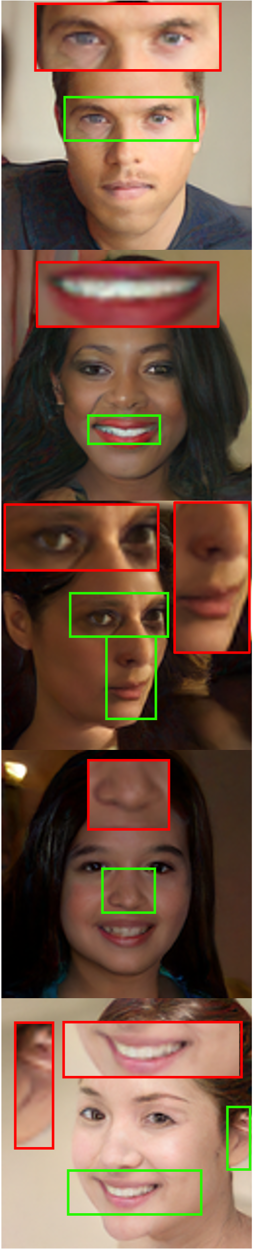
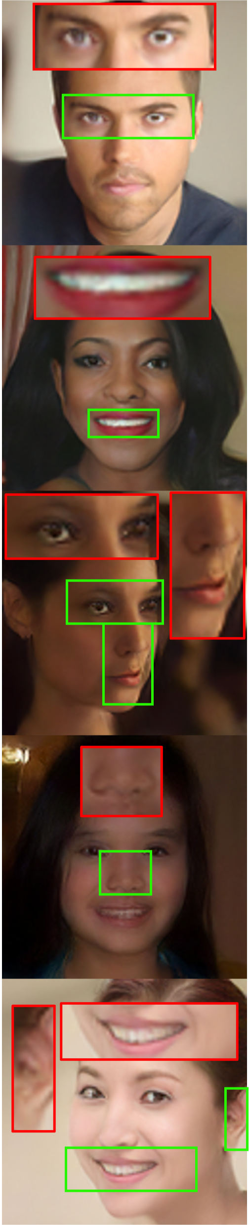
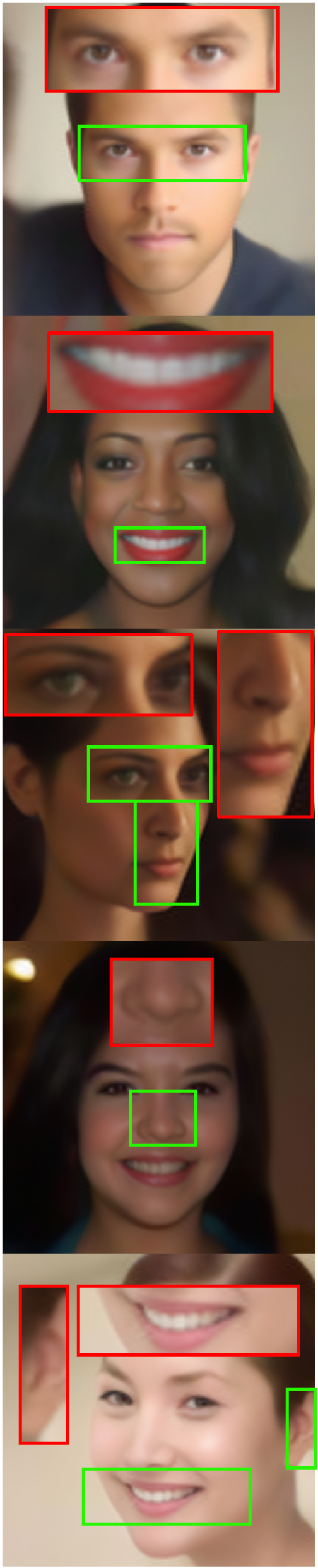
For qualitative comparison, as it can be observed in Figure 3, the generated faces of FDDiff conditioned on LR images contain more realistic facial features, e.g., eyes, teeth, ears, and noses. Although may not being as sharpened as SR3 and IDM, the results of FDDiff contain facial fine-grained details with higher fidelity to the ground truth. Especially for eyes, ears, and teeth, there is a large discrepancy between the results of SR3/IDM and HR images, while FDDiff preserves higher consistency with HR images.
| Methods | Datasets | BSDS100 | General100 | Urban100 | ||||||
| 5 | ||||||||||
| 8 | ||||||||||
| 11 | ||||||||||
| PSNR | SSIM | LPIPS | PSNR | SSIM | LPIPS | PSNR | SSIM | LPIPS | ||
| SRGAN[20] | DIV2K | 24.13 | 0.6454 | 0.1777 | 27.54 | 0.7998 | 0.0961 | 22.84 | 0.7196 | 0.1551 |
| SFTGAN[41] | ImageNet | 24.09 | 0.6460 | 0.1710 | 27.04 | 0.7861 | 0.1084 | 22.74 | 0.7107 | 0.1433 |
| ESRGAN[42] | DF2K | 23.95 | 0.6463 | 0.1615 | 27.53 | 0.7984 | 0.0880 | 22.78 | 0.7214 | 0.1229 |
| RankSRGAN[47] | DIV2K | 24.09 | 0.6438 | 0.1750 | 27.31 | 0.7899 | 0.0960 | 22.93 | 0.7169 | 0.1385 |
| SRFlow[25] | DF2K | 24.66 | 0.6580 | 0.1833 | 27.83 | 0.7951 | 0.0962 | 23.68 | 0.7316 | 0.1272 |
| SPSR[26] | DIV2K | 24.16 | 0.6531 | 0.1613 | 27.65 | 0.7995 | 0.0866 | 23.24 | 0.7365 | 0.1190 |
| SROOE[31] | DIV2K | 24.78 | 0.6818 | 0.1530 | 28.57 | 0.8250 | 0.0764 | 24.21 | 0.7680 | 0.1066 |
| SROOS[31] | DF2K | 25.07 | 0.6960 | 0.1388 | 29.12 | 0.8400 | 0.0682 | 24.53 | 0.7784 | 0.0988 |
| FDDiff | DIV2K | 25.53 | 0.7196 | 0.1342 | 28.03 | 0.8516 | 0.0970 | 24.41 | 0.7968 | 0.1089 |
LR Images

SR Images
HR Images
General Image Super-Resolution To demonstrate the super-resolution quality of FDDiff for general images, FDDiff trained on DIV2K training set is evaluated on DIV2K validation set. The super-resolution quality is assessed by PSNR and SSIM, and is compared with various models, including: regression-based models EDSR[24] and LIIF[3]; VAE-based models LAR-SR[9]; GAN-based models ESRGAN[42] and RankSRGAN[47]; flow-based models SRFlow[25] and HCFlow[23]; diffusion-based models SRDiff[21], DiWa[29], and IDM[7]. As shown in Table 4, FDDiff achieves competitive numerical SR quality and outstanding perceptual SR quality, outperforming previous by at least 0.14dB for PSNR and for SSIM. It reveals that FDDiff prioritizes human perceptual quality, which is achieved through the progressive refinement for the missing high-frequency information of LR images.
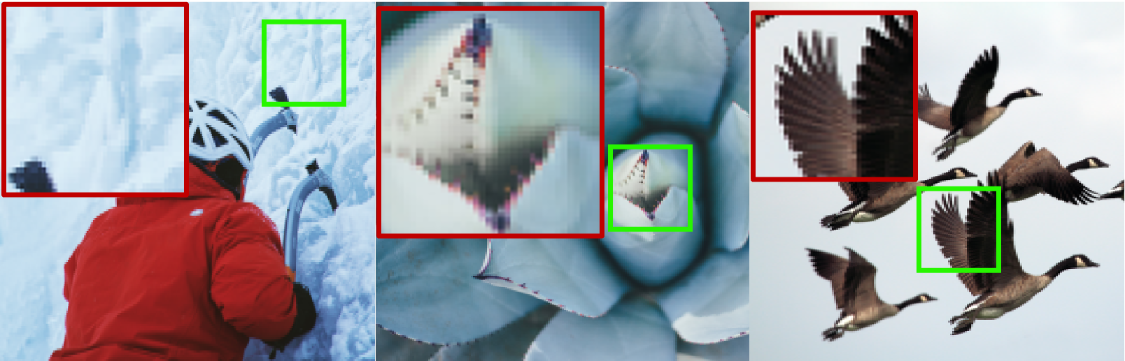
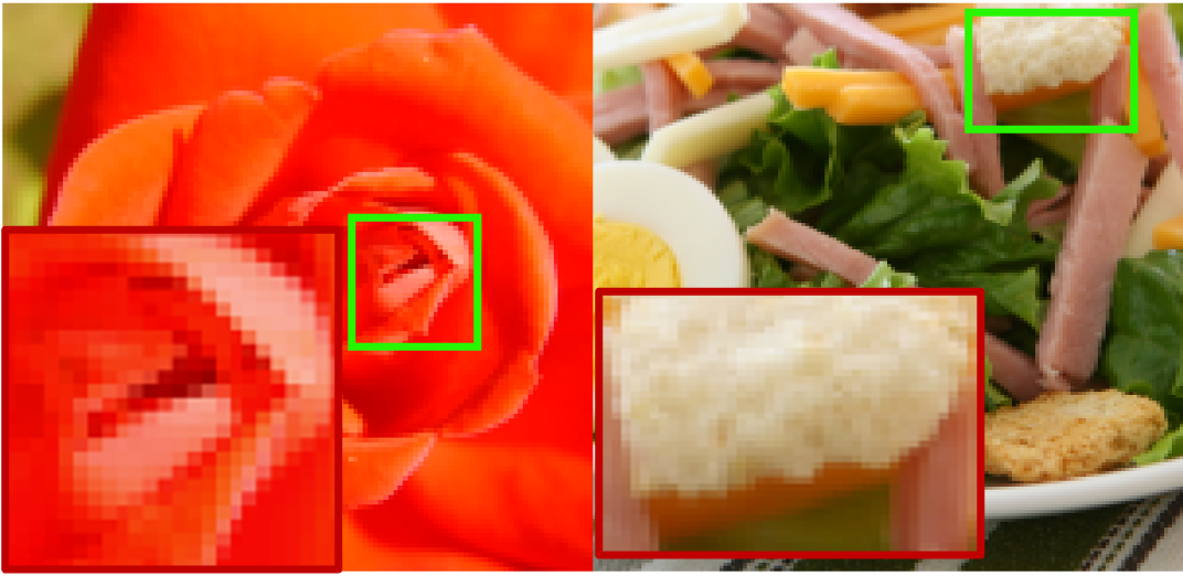
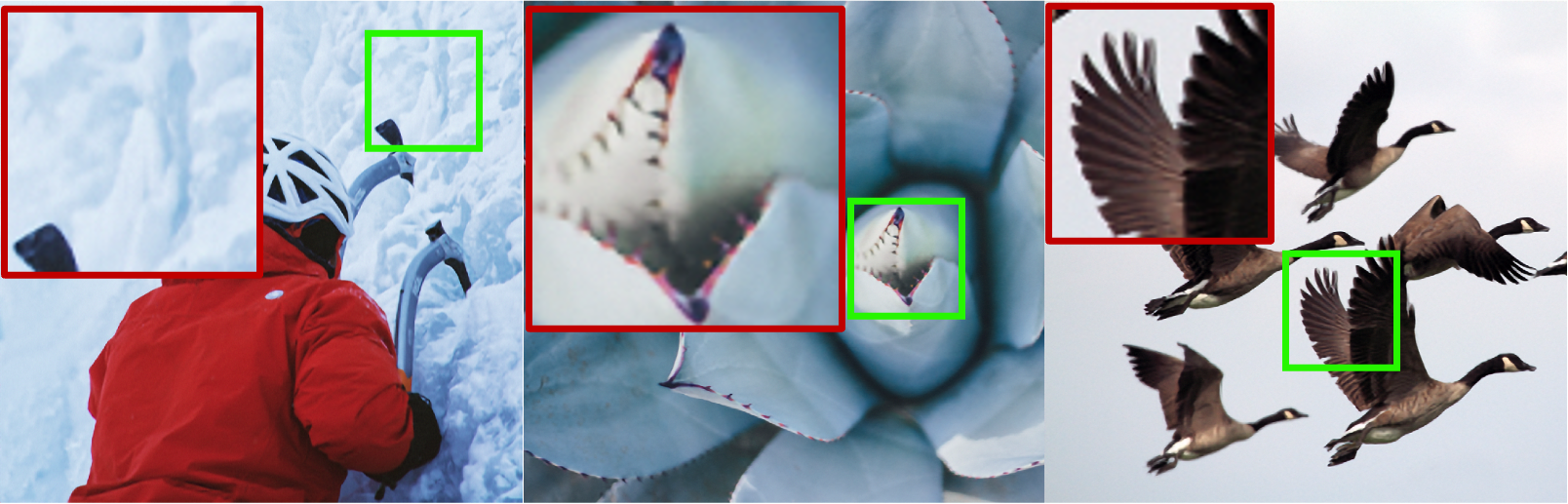
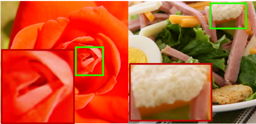
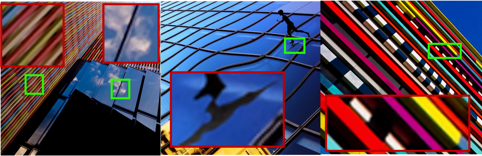
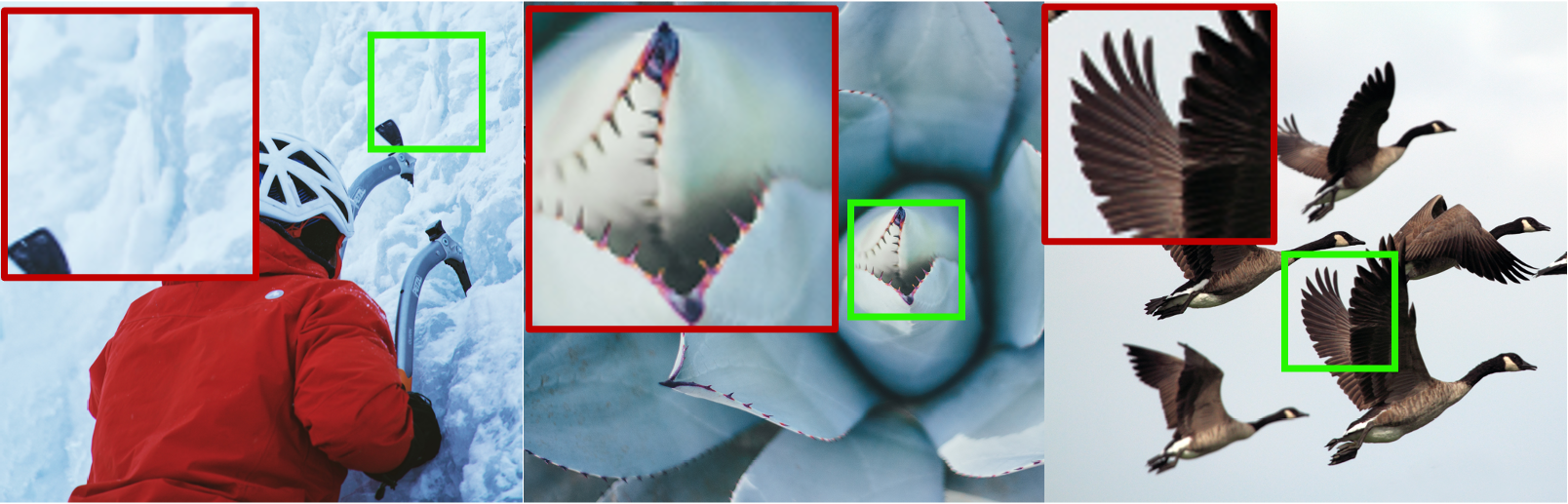
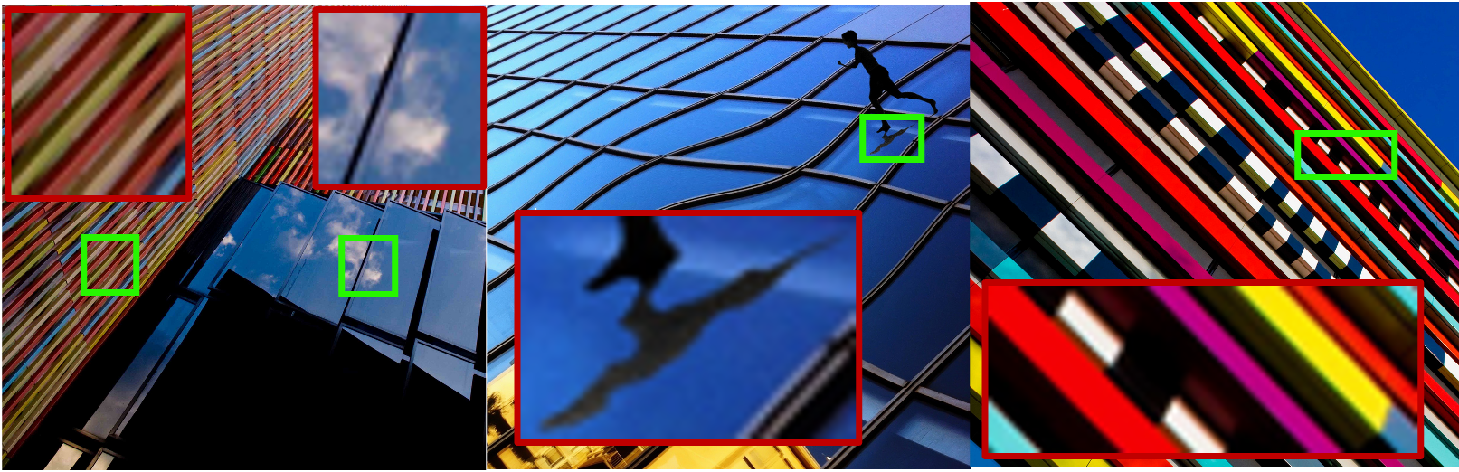
Besides, aiming to illustrate the cross-domain performance of FDDiff for general image super-resolution (), our proposed FDDiff trained on DIV2K is further evaluated on three datasets including BSDS100[27], General100[6], and urban100[14] dataset. Several state-of-the-art generative models are involved in comparison. Quantitative results in Table 5 demonstrate that FDDiff outperforms the baseline in SSIM and yields comparable LPIPS for these three cross-domain datasets, which highlights the versatility of FDDiff. As shown in Figure 4, the qualitative results on 4 SR tasks for general images also demonstrate that FDDiff excels in generating rich high-frequency details, particularly for those images with distinct contours.
Real-world Super-Resolution To further evaluate the performance of FDDiff on real-world 4x SR, we provide an additional quantitative comparison with DASR[44] and StableSR[40] on RealSR(v3) dataset. It is worth noting that StableSR is based on pre-trained Stable Diffusion involving additional large-scale training data which may not be in the same track with us. In Table 4, FDDiff has shown comparable PSNR and SSIM, while not perform well for perceptual metric MUSIQ, where further improvement need to be conducted in future work. Therefore, one of the limitations of FDDiff may lie in its perceptual quality in real-world super-resolution tasks.
4.4 Ablation studies
Effect of Frequency-Domain Refinement Process As shown in Table 6, we construct and evaluate four variants with different scale settings, target numbers, and targets of diffusion process. Similar to prior diffusion-based SR methods[36, 21, 7], Model 1 adapts input layers and output layers of FDDiff to single scale, i.e., the same scale as input images, and only predicts the noise by removing frequency complement chain. Model 2 conducts multistage diffusion and change the target number of FDDiff to , which means a subset of is chosen for the targets . The SR quality of Model 2 is higher than Model 1, demonstrating the effectiveness of our proposed frequency complement chain and the corresponding multiscale frequency refinement diffusion model. Model 3 in the gray row, i.e., FDDiff, has achieved higher SR quality, owing to its fine-grained frequency partition. As for Model 4, it removes the diffusion process to only predict for frequency complement chain, and obtains lower PSNR and SSIM. This proves that the randomness guidance by Gaussian noise in diffusion process is indispensable for high-quality SR.
| No. | Scale Setting | Target Number | Target | PSNR | SSIM | ||||
| 3 | |||||||||
| 6 | |||||||||
| 8 | |||||||||
| Single | Multiple | Single | |||||||
| 1 | ✓ | ✗ | ✓ | ✗ | ✗ | ✓ | ✗ | 24.09 | 0.7002 |
| 2 | ✗ | ✓ | ✗ | ✓ | ✗ | ✓ | ✓ | 24.48 | 0.7092 |
| 3 | ✗ | ✓ | ✗ | ✗ | ✓ | ✓ | ✓ | 24.52 | 0.7116 |
| 4 | ✗ | ✓ | ✗ | ✗ | ✓ | ✗ | ✓ | 21.87 | 0.6046 |
| PSNR | 24.19 | 24.52 |
| Methods | SR3 | IDM | FDDiff |
| Inference time per step | 18.66 ms | 42.09 ms | 17.14 ms |
| Number of parameters | 97.83 M | 116.62 M | 18.21 M |
Effectiveness of Timestep Assignment Schedule To design a monotonic function which is flat for higher t at lower index j and steep for lower t at higher index j, power function is an effective and brief solution. Trigonometric and logarithm function are also feasible with minor revision. The main advantage lies in the comparison with linear schedule, as shown in Table 8.
Trade-off between Generation Speed and Quality Firstly, we conduct comparison on inference efficiency with diffusion-based methods, parameters and total inference time including data processing is evaluated in Table 8.
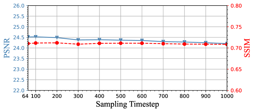
Secondly, since FDDiff is equipped with timestep-skipping sampling procedure of DDIM for more efficient inference, we evaluate the corresponding impacts of sampling timesteps on SR quality. Being trained with total timesteps for SR with upscaling ratio on FFHQ, different sampling timesteps for inference are selected, which should be no less than the number of states, namely . The resulting trade-off between generation speed and quality is shown in Figure 6, which illustrate that FDDiff can achieve decent performance with only timesteps and be chosen as FDDiff. We note that the SR quality of FDDiff reaches the best at 100 timesteps and tends to be stable over all timesteps, which may differ from prior diffusion-based SR models[36, 38]. The reason may lay in the fact that our model is well-trained and the randomness of our diffusion process is limited by the additional intermediate targets, thus relatively not susceptible to the number of total sampling timesteps.
5 Conclusion
In this paper, we present a Frequency Domain-guided multiscale Diffusion model (FDDiff), which is tailored to progressively complement the missing high-frequency information to low-resolution images and achieve higher-quality super-resolution. With the proposed frequency complement chain, FDDiff decompose the difficult process for generating all high-frequency details into finer-grained steps at multiple scales. We further design a multiscale frequency refinement network to handle multiscale frequency complement process within one unified network. Extensive experiments on general and facial images demonstrate the superior performance of FDDiff over prior generative models. In future work, we will develop the frequency-domain sampling schedule for faster inference.
References
- [1] Agustsson, E., Timofte, R.: Ntire 2017 challenge on single image super-resolution: Dataset and study. In: IEEE Conf. Comput. Vis. Pattern Recog. Worksh. pp. 126–135 (2017)
- [2] Cai, J., Zeng, H., Yong, H., Cao, Z., Zhang, L.: Toward real-world single image super-resolution: A new benchmark and a new model. In: Int. Conf. Comput. Vis. (2019)
- [3] Chen, Y., Liu, S., Wang, X.: Learning continuous image representation with local implicit image function. In: IEEE Conf. Comput. Vis. Pattern Recog. pp. 8628–8638 (2021)
- [4] Chen, Y., Tai, Y., Liu, X., Shen, C., Yang, J.: FSRNet: End-to-end learning face super-resolution with facial priors. In: IEEE Conf. Comput. Vis. Pattern Recog. pp. 2492–2501 (2018)
- [5] Dong, C., Loy, C.C., He, K., Tang, X.: Image super-resolution using deep convolutional networks. IEEE Trans. Pattern Anal. Mach. Intell. 38, 295–307 (2015)
- [6] Dong, C., Loy, C.C., Tang, X.: Accelerating the super-resolution convolutional neural network. In: Eur. Conf. Comput. Vis. pp. 391–407 (2016)
- [7] Gao, S., Liu, X., Zeng, B., Xu, S., Li, Y., Luo, X., Liu, J., Zhen, X., Zhang, B.: Implicit diffusion models for continuous super-resolution. In: IEEE Conf. Comput. Vis. Pattern Recog. pp. 10021–10030 (2023)
- [8] Gu, J., Zhai, S., Zhang, Y., Bautista, M.A., Susskind, J.: f-DM: A multi-stage diffusion model via progressive signal transformation. In: Int. Conf. Learn. Represent. (2023)
- [9] Guo, B., Zhang, X., Wu, H., Wang, Y., Zhang, Y., Wang, Y.F.: Lar-sr: A local autoregressive model for image super-resolution. In: IEEE Conf. Comput. Vis. Pattern Recog. pp. 1909–1918 (2022)
- [10] Hang, T., Gu, S., Li, C., Bao, J., Chen, D., Hu, H., Geng, X., Guo, B.: Efficient diffusion training via min-SNR weighting strategy. In: Int. Conf. Comput. Vis. pp. 7441–7451 (2023)
- [11] He, K., Zhang, X., Ren, S., Sun, J.: Deep residual learning for image recognition. In: IEEE Conf. Comput. Vis. Pattern Recog. pp. 770–778 (2016)
- [12] Ho, J., Jain, A., Abbeel, P.: Denoising diffusion probabilistic models. In: Adv. Neural Inform. Process. Syst. pp. 6840–6851 (2020)
- [13] Huang, H., He, R., Sun, Z., Tan, T.: Wavelet-SRNet: A wavelet-based cnn for multi-scale face super resolution. In: Int. Conf. Comput. Vis. pp. 1689–1697 (2017)
- [14] Huang, J.B., Singh, A., Ahuja, N.: Single image super-resolution from transformed self-exemplars. In: IEEE Conf. Comput. Vis. Pattern Recog. pp. 5197–5206 (2015)
- [15] Iandola, F.N., Han, S., Moskewicz, M.W., Ashraf, K., Dally, W.J., Keutzer, K.: SqueezeNet: Alexnet-level accuracy with 50x fewer parameters and 0.5mb model size. arXiv:1602.07360 (2016)
- [16] Karras, T., Aila, T., Laine, S., Lehtinen, J.: Progressive growing of GANs for improved quality, stability, and variation. In: Int. Conf. Learn. Represent. (2018)
- [17] Karras, T., Laine, S., Aila, T.: A style-based generator architecture for generative adversarial networks. In: IEEE Conf. Comput. Vis. Pattern Recog. pp. 4401–4410 (2019)
- [18] Ke, J., Wang, Q., Wang, Y., Peyman, M., Yang, F.: MUSIQ: Multi-scale image quality transformer. In: IEEE Conf. Comput. Vis. Pattern Recog. pp. 1191–1200 (2022)
- [19] Laine, A., Fan, J.: Texture classification by wavelet packet signatures. IEEE Trans. Pattern Anal. Mach. Intell. 15(11), 1186–1191 (1993)
- [20] Ledig, C., Theis, L., Huszár, F., Caballero, J., Cunningham, A., Acosta, A., Aitken, A., Tejani, A., Totz, J., Wang, Z., et al.: Photo-realistic single image super-resolution using a generative adversarial network. In: IEEE Conf. Comput. Vis. Pattern Recog. pp. 4681–4690 (2017)
- [21] Li, H., Yang, Y., Chang, M., Chen, S., Feng, H., Xu, Z., Li, Q., Chen, Y.: SRDiff: Single image super-resolution with diffusion probabilistic models. Neurocomputing 479, 47–59 (2022)
- [22] Li, J., Dai, T., Zhu, M., Chen, B., Wang, Z., Xia, S.T.: FSR: A general frequency-oriented framework to accelerate image super-resolution networks. In: AAAI Conf. Artif. Intell. pp. 1343–1350 (2023)
- [23] Liang, J., Lugmayr, A., Zhang, K., Danelljan, M., Van Gool, L., Timofte, R.: Hierarchical conditional flow: A unified framework for image super-resolution and image rescaling. In: IEEE Conf. Comput. Vis. Pattern Recog. pp. 4076–4085 (2021)
- [24] Lim, B., Son, S., Kim, H., Nah, S., Mu Lee, K.: Enhanced deep residual networks for single image super-resolution. In: IEEE Conf. Comput. Vis. Pattern Recog. Worksh. pp. 136–144 (2017)
- [25] Lugmayr, A., Danelljan, M., Van Gool, L., Timofte, R.: SRFlow: Learning the super-resolution space with normalizing flow. In: Eur. Conf. Comput. Vis. pp. 715–732 (2020)
- [26] Ma, C., Rao, Y., Cheng, Y., Chen, C., Lu, J., Zhou, J.: Structure-preserving super resolution with gradient guidance. In: IEEE Conf. Comput. Vis. Pattern Recog. pp. 7769–7778 (2020)
- [27] Martin, D., Fowlkes, C., Tal, D., Malik, J.: A database of human segmented natural images and its application to evaluating segmentation algorithms and measuring ecological statistics. In: Int. Conf. Comput. Vis. pp. 416–423 (2001)
- [28] Menon, S., Damian, A., Hu, S., Ravi, N., Rudin, C.: Pulse: Self-supervised photo upsampling via latent space exploration of generative models. In: IEEE Conf. Comput. Vis. Pattern Recog. pp. 2437–2445 (2020)
- [29] Moser, B., Frolov, S., Raue, F., Palacio, S., Dengel, A.: Waving goodbye to low-res: A diffusion-wavelet approach for image super-resolution. arXiv:2304.01994 (2023)
- [30] Nichol, A.Q., Dhariwal, P.: Improved denoising diffusion probabilistic models. In: Int. Conf. Mach. Learn. pp. 8162–8171 (2021)
- [31] Park, S.H., Moon, Y.S., Cho, N.I.: Perception-oriented single image super-resolution using optimal objective estimation. In: IEEE Conf. Comput. Vis. Pattern Recog. pp. 1725–1735 (2023)
- [32] Perez, E., Strub, F., De Vries, H., Dumoulin, V., Courville, A.: FiLM: Visual reasoning with a general conditioning layer. In: AAAI Conf. Artif. Intell. pp. 3942–3951 (2018)
- [33] Phung, H., Dao, Q., Tran, A.: Wavelet diffusion models are fast and scalable image generators. In: IEEE Conf. Comput. Vis. Pattern Recog. pp. 10199–10208 (2023)
- [34] Ronneberger, O., Fischer, P., Brox, T.: U-Net: Convolutional networks for biomedical image segmentation. In: Proc. Int. Conf. Med. Image Comput. Comput.-Assisted Intervention. pp. 234–241 (2015)
- [35] Russakovsky, O., Deng, J., Su, H., Krause, J., Satheesh, S., Ma, S., Huang, Z., Karpathy, A., Khosla, A., Bernstein, M., Berg, A.C., Fei-Fei, L.: ImageNet Large Scale Visual Recognition Challenge. Int. J. Comput. Vis. 115, 211–252 (2015)
- [36] Saharia, C., Ho, J., Chan, W., Salimans, T., Fleet, D.J., Norouzi, M.: Image super-resolution via iterative refinement. IEEE Trans. Pattern Anal. Mach. Intell. 45, 4713–4726 (2022)
- [37] Shi, W., Caballero, J., Huszár, F., Totz, J., Aitken, A.P., Bishop, R., Rueckert, D., Wang, Z.: Real-time single image and video super-resolution using an efficient sub-pixel convolutional neural network. In: IEEE Conf. Comput. Vis. Pattern Recog. pp. 1874–1883 (2016)
- [38] Song, J., Meng, C., Ermon, S.: Denoising diffusion implicit models. In: Int. Conf. Learn. Represent. (2020)
- [39] Vaswani, A., Shazeer, N., Parmar, N., Uszkoreit, J., Jones, L., Gomez, A.N., Kaiser, Ł., Polosukhin, I.: Attention is all you need. Adv. Neural Inform. Process. Syst. pp. 6000–6010 (2017)
- [40] Wang, J., Yue, Z., Zhou, S., Chan, K.C., Loy, C.C.: Exploiting diffusion prior for real-world image super-resolution. arXiv:2305.07015 (2023)
- [41] Wang, X., Yu, K., Dong, C., Loy, C.C.: Recovering realistic texture in image super-resolution by deep spatial feature transform. In: IEEE Conf. Comput. Vis. Pattern Recog. pp. 606–615 (2018)
- [42] Wang, X., Yu, K., Wu, S., Gu, J., Liu, Y., Dong, C., Qiao, Y., Change Loy, C.: ESRGAN: Enhanced super-resolution generative adversarial networks. In: Eur. Conf. Comput. Vis. Worksh. (2018)
- [43] Wang, Z., Bovik, A.C., Sheikh, H.R., Simoncelli, E.P.: Image quality assessment: from error visibility to structural similarity. IEEE Trans. Image Process. 13, 600–612 (2004)
- [44] Wei, Y., Gu, S., Li, Y., Timofte, R., Jin, L., Song, H.: Unsupervised real-world image super resolution via domain-distance aware training. In: IEEE Conf. Comput. Vis. Pattern Recog. pp. 13385–13394 (2021)
- [45] Yang, S., Wu, T., Shi, S., Lao, S., Gong, Y., Cao, M., Wang, J., Yang, Y.: MANIQA: Multi-dimension attention network for no-reference image quality assessment. In: IEEE Conf. Comput. Vis. Pattern Recog. pp. 1191–1200 (2022)
- [46] Zhang, R., Isola, P., Efros, A.A., Shechtman, E., Wang, O.: The unreasonable effectiveness of deep features as a perceptual metric. In: IEEE Conf. Comput. Vis. Pattern Recog. (2018)
- [47] Zhang, W., Liu, Y., Dong, C., Qiao, Y.: RankSRGAN: Generative adversarial networks with ranker for image super-resolution. In: Int. Conf. Comput. Vis. pp. 3096–3105 (2019)
- [48] Zhong, Z., Shen, T., Yang, Y., Lin, Z., Zhang, C.: Joint sub-bands learning with clique structures for wavelet domain super-resolution. Adv. Neural Inform. Process. Syst. pp. 165–175 (2018)