Charged rotating wormholes: charge without charge

$\mbox{Hyeong-Chan\,\, Kim}^{\P}$,   $\mbox{Sung-Won \,\, Kim}^{{\ddagger}}$,   $\mbox{Bum-Hoon \,\, Lee}^{\S{\dagger}}$,   $\mbox{Wonwoo \,\, Lee}^{\S}$,

§Center for Quantum Spacetime, Sogang University, Seoul 04107, Korea
†Department of Physics, Sogang University, Seoul 04107, Korea
¶School of Liberal Arts and Sciences, Korea National University of Transportation, Chungju 27469, Korea
‡Ewha Womans University, Seoul 03760, Korea

Abstract

We present a family of charged rotating wormhole solutions to the Einstein-Maxwell equations, supported by anisotropic matter fields. We first revisit the charged static cases and analyze the conditions for the solution to represent a wormhole geometry. The rotating geometry is obtained by applying the Newman-Janis algorithm to the static geometry. We show the solutions to Maxwell equations in detail. We believe that our wormhole geometry offers a geometric realization corresponding to the concept of ’charge without charge’.

1 Introduction

Einstein’s theory of gravitation [1] has been verified by many experimental tests [2, 3, 4, 5] over $100$ years and has reached a mature stage as a theory of gravitation. The lack of a clear explanation for dark matter and dark energy is sparking interest in modified theories of gravitation, and the need for accurate descriptions of astrophysical phenomena continues to drive interest in finding and analyzing various solutions with matter fields beyond the vacuum solution.

As one of the most fantastical solutions allowed by the theory of gravitation, the wormhole solution [6], allowing time travel [7, 8, 9, 10], has become an object of interest and awes for scientists and the public alike, as well as a great subject for study, fiction, and movies [11].

For this reason, the study of traversable wormholes is becoming more popular. It is also important to examine the possibility of travel by checking whether the tidal force felt by the traveler (spacecraft) near the throat of the wormhole is comparable to Earth’s gravity [6]. This tidal effect would appear as the Riemann tensor components in general relativity. We also should check the flare-out condition and how the geometry differs from that of a black hole. Of course, there should be no physical singularities in the wormhole geometry.

Einstein and Rosen first studied wormhole physics seriously [12], in which they considered a bridge connecting two identical sheets. To see the history of wormhole physics in detail, consult Refs. [13, 14]. Wormhole physics received a modern boost with the paper by Morris and Thorne [6] and has been extensively studied, with wormholes being constructed and studied in various modified theories of gravitation [15, 16, 17, 18, 19, 20, 21, 22, 23, 24, 25] and dimensions [26, 27, 28, 29, 30]. The role of fermion fields on the wormhole geometry [20, 31, 32, 33, 34] has also been studied.

To construct and maintain wormholes, special matter fields are required. This matter is also related to the flare-out condition for the wormhole throat and, as a result, one should study the energy condition for those matter fields. In Einstein’s theory, it is well known that the construction of a wormhole requires matter that does not satisfy the null energy condition, e.g. phantom energy [35]. In modified gravity theories, the modified gravity effect can also play the role of these fields.

The wormhole geometry can be an example of a geometric realization corresponding to the concept of ‘charge without charge’ as the solution to source-free Maxwell equations when given as the solution to a travelable wormhole. In connection with the concept of ‘charge without charge’, Misner and Wheeler emphasized the significance of the solution to the source-free Maxwell equations  [36], where the electric field enters one side of the wormhole and exits the other side. This concept will be realized if one finds a charged wormhole solution [37]. Even though the Maxwell field is not a necessary matter field to construct a wormhole, it will be interesting to study how its effects affect the wormhole geometry. This addition of matter fields increases the number of equations of motion, which could be solved analytically or numerically to find their solutions. In this paper, we wish to construct the charged rotating wormhole geometry with an anisotropic matter field [38, 39] and find the Maxwell solution analytically for this geometry. In particular, we will consider the wormhole with the anisotropic matter field obtained in Ref. [39].

We are also interested in the geometry supported by rotating objects and have been studying rotating black holes [40, 41]. Since the discovery of the Kerr black hole [42], continuing efforts to find solutions for rotating black holes [43, 44, 45, 46, 40], either by applying the Newman-Janis (NJ) algorithm  [47, 43] or the method in the Ref. [48]. Usually, studies of rotating wormholes have been done by assuming metric ansatz [49, 50, 51, 52, 53, 54]. In this work, we employ the NJ algorithm to find a rotating wormhole solution starting from a charged static wormhole solution obtained from solving the Einstein-Maxwell equations. Since the NJ algorithm corresponds to the solution of the rotating geometry, i.e., Einstein equations, we should solve Maxwell equations additionally to obtain the Maxwell tensor in the rotating geometry. We present the Maxwell tensor satisfying the Maxwell equations in our rotating wormhole geometry.

This paper is organized as follows: In Sec. [2], we show the charged static wormhole solution, and the energy density and pressure of the matter fields to support this wormhole geometry. We analyze the conditions for our solutions to be the traversable wormhole in detail. In Sec. [3], we employ the NJ algorithm and present the charged rotating wormhole solution. In Sec. [4], we summarize and discuss our results.

2 Charged static wormhole

In this section, we construct traversable charged static wormhole solutions. We first solve both Einstein and Maxwell equations coupled with a matter field. We then analyze conditions for the geometry to be a wormhole.

2.1 Setup and solution

We consider the action

$$I=\int d^{4}x\sqrt{-g}\Big{[}\frac{1}{16\pi}(R-F_{\mu\nu}F^{\mu\nu})+{\cal L}_{\rm am}\Big{]}+I_{\rm b},$$ (1)

where ${\cal L}_{\rm am}$ describes effective anisotropic matter fields,$I_{\rm b}$ is the boundary term [55, 56], and we take $G=1$ for simplicity.

Varying the action, we obtain the Einstein equation

$$G_{\mu\nu}=R_{\mu\nu}-\frac{1}{2}Rg_{\mu\nu}=8\pi T_{\mu\nu}\,,$$ (2)

where the stress-energy tensor takes the form

$$T^{\mu\nu} = T^{\mu\nu}_{\rm M}+T^{\mu\nu}_{\rm am}$$ (3)

$$= \frac{1}{4\pi}(F^{\mu}_{~{}\alpha}F^{\nu\alpha}-\frac{1}{4}g^{\mu\nu}F_{\alpha\beta}F^{\alpha\beta})+(\varepsilon_{\rm am}+p_{t{\rm am}})u^{\mu}u^{\nu}+p_{t{\rm am}}g^{\mu\nu}+(p_{r{\rm am}}-p_{t{\rm am}})x^{\mu}x^{\nu}\,,$$

where $\varepsilon_{\rm am}$ is the energy density of the anisotropic matter, $u^{\mu}$ is four-velocity, and $x^{\mu}$ is a spacelike unit vector, respectively. The radial and the transverse (lateral) pressures are assumed to be linearly proportional to the energy density:

$$p_{r{\rm am}}=w_{\rm 1}\varepsilon_{\rm am}\,,~{}~{}~{}p_{t{\rm am}}=w_{\rm 2}\varepsilon_{\rm am}\,,$$ (4)

then stress tensor for the anisotropic matter field in Eq. (3) can be rewritten as $T^{\mu}_{\nu{\rm am}}={\rm diag}(-\varepsilon_{\rm am},w_{1}\varepsilon_{\rm am},w_{2}\varepsilon_{\rm am},w_{2}\varepsilon_{\rm am})$. The source-free Maxwell equations are given by

$$\nabla_{\nu}F^{\mu\nu}=\frac{1}{\sqrt{-g}}[\partial_{\nu}(\sqrt{-g}F^{\mu\nu})]=0\,.$$ (5)

We take the metric for the static spherically symmetric charged wormhole geometry

$$ds^{2}=-f(r)dt^{2}+\frac{1}{g(r)}dr^{2}+r^{2}(d\theta^{2}+\sin^{2}\theta d\psi^{2})\,,$$ (6)

where metric functions $f(r)$ and $g(r)$ denote the redshift function and include the wormhole shape function, respectively. We consider an asymptotically flat spacetime.

After solving the Maxwell and Einstein equations, we analyze the conditions for the solution to be a travelable wormhole.

Let us first tackle the Maxwell equation. For the electrically charged static geometry, $F^{tr}=E^{r}=\sqrt{\frac{g(r)}{f(r)}}\frac{Q}{r^{2}}$ satisfy the source-free Maxwell equations (5). In the asymptotic rest frame, one could measure the electric field. That field should be defined in an orthonormal frame, we adopt covariant tetrad shown as $e^{\hat{t}}_{\mu}=(\sqrt{f(r)},0,0,0)$, $e^{\hat{r}}_{\mu}=(0,\frac{1}{\sqrt{g(r)}},0,0)$, $e^{\hat{\theta}}_{\mu}=(0,0,r,0)$, and $e^{\hat{\psi}}_{\mu}=(0,0,0,r\sin\theta)$. The electric field takes the form of $F^{{\hat{a}}{\hat{b}}}=e^{\hat{a}}_{\mu}e^{\hat{b}}_{\nu}F^{\mu\nu}$, which gives $E^{\hat{r}}=\frac{Q}{r^{2}}$.

We take the metric functions $f(r)=\left(1+\frac{Q^{2}}{r^{2}}\right)$ and $g(r)=\left(1+\frac{Q^{2}}{r^{2}}-\frac{b(r)}{r}\right)$ in Ref. [37]. This geometry has the minimum radius at the throat $r=r_{o}$, i.e. $b(r)=b_{o}$ at $r_{o}$ and thus $g(r_{o})=0$. This gives $b_{o}=(r^{2}_{o}+Q^{2})/r_{o}$, in which $b_{o}$ is the physical parameter of the wormhole with given $w_{1}$. When $Q$ and $b_{o}$ are given, there are two locations of the throat, $r_{o}=\frac{1}{2}(b_{o}\pm\sqrt{b^{2}_{o}-4Q^{2}})$. We take the larger one as

$$r_{o}=\frac{1}{2}(b_{o}+\sqrt{b^{2}_{o}-4Q^{2}})\,,$$ (7)

and $b_{o}>2Q$. If $b_{o}=2Q$, then $r_{o}=Q$, which will not satisfy the flare-out condition for later analysis. When $Q$ vanishes, $b_{o}=r_{o}$. The presence of charge $Q$ reduces the size of the wormhole throat.

There exists also a solution that satisfies Einstein’s equations in the region $r\leq r_{o}$, in which $r_{o}$ is the smaller one. This solution will give a geometry describing $0<r\leq r_{o}$. At $r=0$, it will have a singularity, and at $r=r_{o}$, it will give a geometry connected by a wormhole. We leave the analysis of this part to future work.

We now consider Einstein equations. The nonvanishing components of the Einstein tensor are given by

$$G^{t}_{t} = -8\pi\varepsilon=8\pi(-\varepsilon_{c}-\varepsilon_{\rm am})=8\pi(-\varepsilon_{c})-\frac{b^{\prime}(r)}{r^{2}}\,,$$ (8)

$$G^{r}_{r} = 8\pi p_{r}=8\pi(-\varepsilon_{c}+w_{1}\varepsilon_{\rm am})=8\pi(-\varepsilon_{c})+\frac{(Q^{2}-r^{2})b(r)}{r^{3}(Q^{2}+r^{2})}\,,$$ (9)

$$G^{\theta}_{\theta} = 8\pi p_{t}=8\pi(\varepsilon_{c}+w_{2}\varepsilon_{\rm am})$$ (10)

$$= 8\pi(\varepsilon_{c})+\frac{1}{2r^{3}(Q^{2}+r^{2})^{2}}[(-2Q^{4}-3Q^{2}r^{2}+r^{4})b(r)-r^{3}(Q^{2}+r^{2})b^{\prime}(r)]\,,$$

where $\varepsilon_{c}=\frac{Q^{2}}{8\pi r^{4}}$, $p_{r}$ is the radial pressure, $p_{t}$ is the transverse pressure, and the prime denotes the derivative with respect to $r$.

From Eqs. (8) and (9), we obtain

$$b(r)=b_{o}\left(\frac{rb_{o}}{r^{2}+Q^{2}}\right)^{1/w_{1}}\,.$$ (11)

Substituting this result back into Eqs. (8) or (9), we get $\varepsilon_{\rm am}=-\frac{r^{2}-Q^{2}}{8\pi w_{1}r^{4}}\left(\frac{b_{o}r}{r^{2}+Q^{2}}\right)^{(w_{1}+1)/w_{1}}$. After plugging those into Eq. (10), we obtain

$$w_{2}(r)=\frac{[-r^{4}(1+w1)+Q^{2}r^{2}(1+3w_{1})+2Q^{4}w_{1}]}{2(r^{4}-Q^{4})}\,.$$ (12)

Then, the energy density and pressures are given by

$$\varepsilon = \frac{Q^{2}}{8\pi r^{4}}-\frac{r^{2}-Q^{2}}{8\pi w_{1}r^{4}}\left(\frac{b_{o}r}{r^{2}+Q^{2}}\right)^{(w_{1}+1)/w_{1}}\,,$$

$$p_{r} = -\frac{Q^{2}}{8\pi r^{4}}-\frac{r^{2}-Q^{2}}{8\pi r^{4}}\left(\frac{b_{o}r}{r^{2}+Q^{2}}\right)^{(w_{1}+1)/w_{1}}\,,$$ (13)

$$p_{t} = \frac{Q^{2}}{8\pi r^{4}}+\frac{1}{16\pi r^{4}(r^{2}+Q^{2})}\left(\frac{b_{o}r}{r^{2}+Q^{2}}\right)^{(w_{1}+1)/w_{1}}\frac{[r^{4}(1+w_{1})-Q^{2}(r^{2}(1+3w_{1})+2Q^{2}w_{1})]}{w_{1}}\,.$$

We could not exactly separate the energy density and the pressure of the charge contribution from the anisotropic matter contribution. When reducing $Q=0$, the results are reduced to the wormhole with $Q=0$ [37, 38, 39].

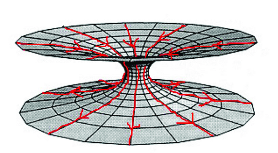
Figure 1: (color online). Conceptual embedded diagram of the wormhole with electric field lines.

Figure 1 represents a conceptual embedded diagram of the wormhole with electric field lines. In this diagram, electric field lines of red color converge on a wormhole from one universe, pass through the wormhole, and exit into the other universe. At the throat, the Maxwell tensor, $F^{tr}=\sqrt{\frac{g(r)}{f(r)}}\frac{Q}{r^{2}}$, goes to zero, ensuring continuity of the value across the throat. If one takes a Gaussian surface, which surrounds the asymptotic regions of both universes, there is the flux of an electric field coming out as there is going in, thus there exists no real charge within the Gaussian surface. As a result, this fact represents the concept of ’charge without charge’.

2.2 Conditions to be a wormhole geometry

Now let us describe the conditions that the above solution to Einstein-Maxwell equations describes a wormhole geometry.

$\bullet$ First, let us look at metric functions. The metric functions, $f(r)$ and $g(r)$, are not the same. If they were [57, 58, 59, 60, 61, 62, 63], the radial pressure could be the negative of the energy density [64]. This is simply recognized by checking the relation $p_{r}+\varepsilon=\frac{g(r)f^{\prime}(r)-f(r)g^{\prime}(r)}{rf(r)}$. Equations (8) and (9) do not satisfy this relation, except for the case $w_{1}=-1$.

Unlike black hole geometry, wormhole geometry must not have an event horizon or a physical singularity. These are related to the properties of $f(r)$ and $g(r)$. For a black hole spacetime, the location of the event horizon is where both functions $f(r)$ and $g(r)$ go to zero simultaneously. The former is for a Killing vector field being null, while the latter is for $r={\rm const}$ surface being null. The infinite redshift surface is also obtained at the location of the vanishing $f(r)$. There exist three invariant curvature scalars, i.e., $R$, $R_{\mu\nu}R^{\mu\nu}$, and $R_{\mu\nu\alpha\beta}R^{\mu\nu\alpha\beta}$. The denominator of these functions consists of the power of $f(r)$, and the function $g(r)$ does not appear in the denominator. It is also possible if the position of $f(r)=0$ as the infinite redshift surface is smaller than the wormhole throat. Our wormhole spacetime covers from the location of the throat, $r=r_{o}$, to infinity. Then, it would be an undefined position in the wormhole geometry. Therefore, $f(r)$ is non-zero and positive finite at $r\geq r_{o}$. This condition also ensures that there is no physical singularity at $r\geq r_{o}$. A rotating version of this type of wormhole would have an ergosphere.

Now let us examine the physical meaning of spacetime at the point where the metric function $g(r)$ vanishes. These points appear in the geometry of both black holes and wormholes and should be described separately. The closed two-dimensional spatial hypersurface at that location corresponds to a marginally trapped surface for a dynamic black hole [65, 66, 67], while to a marginally anti-trapped surface for a dynamic wormhole [68, 69]. It corresponds to the coordinate singularity. One could consider the proper radial distance, $l(r)=\pm\int^{r}_{r_{o}}\frac{dr}{\sqrt{g(r)}}$, is required to be finite everywhere. For our wormhole, the condition $g(r)=0$ can have multiple roots, and we want $g(r)$ to be non-negative near the throat and at that. Thus we take the largest root as the location of the throat and assume it is assumed to be the marginally anti-trapped surface.

$\bullet$ Second, let us check out the flare-out condition [6, 70, 68, 71], and the energy condition. To construct and maintain the structure of the traversable wormhole, the geometric flare-out condition must be satisfied at the throat and its neighborhood, which is related to the energy condition of the matter supporting the wormhole structure. It was pointed out that the divergence property of the null geodesic at the marginally anti-trapped surface generalizes the flare-out condition [68]. In this paper, we examine the flare-out condition and the exoticity function at the throat and its neighborhood. We describe how the two conditions relate at and near the wormhole throat. We first consider the flare-out condition of the wormhole through the embedding geometry at $t=\rm const.$ and $\theta=\frac{\pi}{2}$. The condition is given by the minimality of the throat as

$$\frac{d^{2}r}{dz^{2}}=\frac{r[r(b(r)-rb^{\prime}(r))-2Q^{2}]}{2(rb(r)-Q^{2})^{2}}>0\,,$$ (14)

thus the flare-out condition could be determined by $b(r)$ around the throat.

Substituting Eq. (11) into the flare-out condition, we get the numerator as

$$N(r)\equiv-2Q^{2}+\frac{\left(\frac{r(r^{2}_{o}+Q^{2})}{r_{o}(r^{2}+Q^{2})}\right)^{1+1/w_{1}}(Q^{2}(-1+w_{1})+r^{2}(1+w_{1}))}{w_{1}}>0\,.$$ (15)

At the throat, this function turns out to be

$$N(r_{o})=(r^{2}_{o}-Q^{2})\left(1+1/w_{1}\right)>0\,.$$ (16)

Here, we choose $w_{1}>0$ or $w_{1}<-1$ for the asymptotically flat spacetime, which requires the charge to satisfy $r_{o}>Q$ through the flare-out condition as Eq. (16). We obtained the constraint for $Q$ here, and the existence of $Q$ does not modify the range of $w_{1}$ to satisfy the flare-out condition.

One can introduce the exoticity function [6, 71] as

$$\zeta(r)\equiv\frac{-p_{r}-\varepsilon}{|\varepsilon|}=\frac{(r^{2}-Q^{2})(1+w_{1})\left(\frac{rb_{o}}{r^{2}+Q^{2}}\right)^{(w_{1}+1)/w_{1}}}{r^{2}w_{1}}\,.$$ (17)

When the exoticity function is positive, the null energy condition is violated. At the throat, this one becomes

$$\zeta(r_{o})=\frac{(r^{2}_{o}-Q^{2})(1+1/w_{1})}{r^{2}_{o}}\,,$$ (18)

where $\zeta(r_{o})$ takes the same form as (16) up to a positive definite multiplication factor. Thus, the wormhole supported by that matter could satisfy the flare-out condition. When $Q$ vanishes, Eqs. (14) and (17) are proportional.

$\bullet$ Third, let us analyze the traversability condition through the tidal force caused by the wormhole. The tidal forces at and near the wormhole stretch and compress a traveler. For the traveler to travel through that safely, the magnitude of the tidal force felt by the traveler must be within tolerable limits. We consider a traveler traveling through the inside of a wormhole with speed $u^{\hat{\mu}}$ in the orthonormal basis of the static observer. Two points separated by the length of the traveler as the separation vector $\xi^{\hat{k}}$ will not have the same acceleration because of the inhomogeneity of the gravitation. This difference $\triangle a^{\hat{j}}$ is referred to as the tide. Thus the tidal effect is given by [6, 13, 14, 72]

$$\triangle a^{\hat{j}^{\prime}}=-R^{\hat{j}^{\prime}}_{\hat{0}^{\prime}\hat{k}^{\prime}\hat{0}^{\prime}}\xi^{\hat{k}^{\prime}}\,,$$ (19)

where $u^{\hat{\mu}^{\prime}}=\delta^{\hat{\mu}^{\prime}}_{\hat{0}^{\prime}}$ and $\xi^{\hat{0}^{\prime}}=0$ in the traveler’s frame were used. The relation between traveler’s orthonormal basis $e_{\hat{0}^{\prime}},e_{\hat{1}^{\prime}},e_{\hat{2}^{\prime}},e_{\hat{3}^{\prime}}$ and the static observer’s orthonormal basis $e_{\hat{t}},e_{\hat{t}},e_{\hat{\theta}},e_{\hat{\phi}}$ are shown in Ref. [6]. The components of the Riemann tensor are given by

$$R_{\hat{1}^{\prime}\hat{0}^{\prime}\hat{1}^{\prime}\hat{0}^{\prime}} = \frac{f(r)f^{\prime}(r)g^{\prime}(r)-g(r)[f^{\prime 2}(r)-2f(r)f^{\prime\prime}(r)]}{4f^{2}(r)}\,,$$

$$R_{\hat{2}^{\prime}\hat{0}^{\prime}\hat{2}^{\prime}\hat{0}^{\prime}} = R_{\hat{3}^{\prime}\hat{0}^{\prime}\hat{3}^{\prime}\hat{0}^{\prime}}=\frac{\gamma^{2}[g(r)f^{\prime}(r)-v^{2}f(r)g^{\prime}(r)]}{2rf(r)}\,,$$ (20)

where $\gamma=(1-v^{2})^{-1/2}$ and $v=\pm\frac{\sqrt{g_{rr}}dr}{\sqrt{-g_{tt}}dt}$ is the radial velocity of the traveler. Thus, the tidal acceleration becomes at the throat

$$\triangle a^{\hat{1}^{\prime}}|_{r_{o}} = \frac{Q^{2}(1+w_{1})(r^{2}_{o}-Q^{2})}{2w_{1}r^{4}_{o}(r^{2}_{o}+Q^{2})}\xi^{\hat{1}^{\prime}}|_{r_{o}}\,,$$

$$\triangle a^{\hat{2}^{\prime}}|_{r_{o}} = \triangle a^{\hat{3}^{\prime}}|_{r_{o}}=\frac{\gamma^{2}_{o}v^{2}_{o}(1+w_{1})(r^{2}_{o}-Q^{2})}{2r^{4}_{o}w_{1}}\xi^{\hat{2}^{\prime}}|_{r_{o}}\,,$$ (21)

where $\gamma_{o}$ and $v_{o}$ denote those at the throat. The function $f(r)$ constrains the radial component, $\triangle a^{\hat{1}^{\prime}}|_{r_{o}}$, in which the radial component vanishes for $Q=0$ as anticipated [6]. Therefore, if the wormhole has a small $Q$, the traveler could feel the radial component is within the tolerable limit. On the other hand, the speed of $v$ which the traveler crosses the wormhole constrains the lateral component, $\triangle a^{\hat{2}^{\prime}}|_{r_{o}}$. Alternatively, one could consider $|\triangle a|=\sqrt{\sum_{k}(\triangle a^{k})^{2}}$ and compare it with Earth’s gravity, $g_{\bigoplus}=9.8[{\rm m/s^{2}}]$.

$$\frac{|\triangle a|}{g_{\bigoplus}}\leq|1+1/w_{1}|\left(1-\frac{kGQ^{2}}{c^{4}r^{2}_{o}}\right)\sqrt{\frac{k^{2}G^{2}Q^{4}}{(c^{4}r^{2}_{o}+kGQ^{2})^{2}}+2\gamma^{4}_{o}(v_{o}/c)^{4}}\frac{c^{2}|\xi|}{2r^{2}_{o}g_{\bigoplus}}<1\,,$$ (22)

where we recovered the speed of light, $c=3\times 10^{8}[{\rm m/s}]$, the gravitational constant, $G=6.67\times 10^{-11}[{\rm N\cdot m^{2}/kg^{2}}]$, and Coulomb’s constant, $k=9\times 10^{9}[{\rm N\cdot m^{2}/C^{2}_{\rm Cou}}]$. We take the size of the traveler’s body $|\xi|\sim 2[{\rm m}]$.

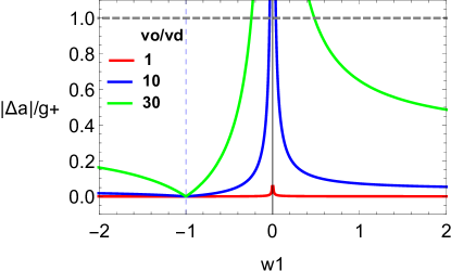
(a) The magnitude as varying $v_{o}$

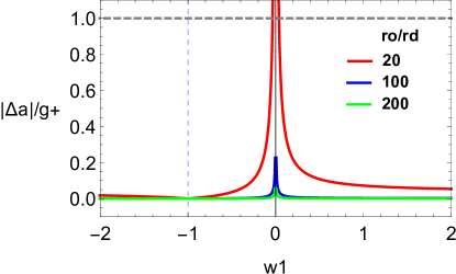
(b) The magnitude as varying $r_{o}$

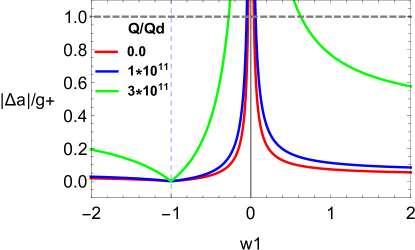
(c) The magnitude as varying $Q$

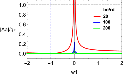
(d) The magnitude as varying $b_{o}$

Figure 2: (color online). The magnitude of tidal accelerations at the throat. The $v_{d}$, $r_{d}$, and $Q_{d}$ are introduced to make dimensionless quantities with the unit quantity.

Figure 2 represents the magnitude of the tidal acceleration at the throat Eq. (22). There are four parameters that we can control. They are the charge $Q$, the traveler’s velocity $v_{o}$, the size of the wormhole throat $r_{o}$, and the size of the traveler $|\xi|$, respectively. We fixed the size of the traveler. As one can see through the Eq. (22), the term $\frac{kGQ^{2}}{c^{4}r^{2}_{o}}\ll 1$, and the first term is much smaller than than the second term in the square root. We do not consider the region $-1\leq w_{1}\leq 0$, and we drew a dashed blue line to mark the location of $w_{1}=-1$.

In the figure $(a)$, we check the magnitude for three different values of $v_{o}$. The red curve represents $v_{o}=1[{\rm m/s}]$, blue represents $v_{o}=10[{\rm m/s}]$, and green represents $v_{o}=30[{\rm m/s}]$, respectively. We take $r_{o}=20[{\rm m}]$. As expected, the magnitude of the tidal acceleration increases with the traveler’s velocity. For wormholes with values of $w_{1}<-1$, the magnitude is small enough. For wormholes with values of $w_{1}>0$, the magnitude is large enough to endanger the traveler for small values of $w_{1}$ and is small enough to allow the traveler to pass through the wormhole safely for large $w_{1}$. In $(b)$, we check the magnitude for three different values of $r_{o}$. The red curve represents $r_{o}=20[{\rm m}]$, blue represents $r_{o}=100[{\rm m}]$, and green represents $r_{o}=200[{\rm m}]$, respectively. We take $v_{o}=10[{\rm m/s}]$ and $Q=1[{\rm C_{Cou}}]$. As expected, the magnitude of the acceleration increases as the size of a wormhole decreases. The general behavior of the curves looks similar to the one in the figure $(a)$. In $(c)$, we check the magnitude for three different values of $Q$. The red curve represents $Q=0[{\rm C_{Cou}}]$, blue represents $Q=10^{11}[{\rm C_{Cou}}]$, and green represents $Q=3\times 10^{11}[{\rm C_{Cou}}]$, respectively. We take $v_{o}=10[{\rm m/s}]$ and $r_{o}=20[{\rm m}]$. As expected, the magnitude of the tidal acceleration increases with the increasing $Q$. If we continue to increase $Q$ so that the ratio of the decrease in the term in the numerator in front of the square root is larger compared to the ratio of the increase in the square root in Eq. (22), the magnitude of the tidal acceleration will decrease again. However, we did not check that because the $Q$ is too large. In $(d)$, we check the magnitude for three different values of $b_{o}$. The red curve represents $b_{o}=20[{\rm m}]$, blue represents $b_{o}=100[{\rm m}]$, and green represents $b_{o}=200[{\rm m}]$, respectively. We take $v_{o}=10[{\rm m/s}]$ and $Q=1[{\rm C_{Cou}}]$. The curves have almost the same behavior.

3 Charged rotating wormhole

In this section, we obtain charged rotating wormhole solution from the static solution via the NJ algorithm.

3.1 The NJ algorithm

We begin with the retarded Eddington-Finkelstein coordinates

$$ds^{2} = -f(r)du^{2}-\frac{2\sqrt{f(r)}dudr}{\sqrt{g(r)}}+r^{2}d\Omega^{2}\,.$$ (23)

We take the null tetrad $\{l_{\mu},n_{\mu},m_{\mu},\bar{m}_{\mu}\}$ consisted of two real null vectors, $l_{\mu}$ and $n_{\mu}$, and a pair of complex null vectors, $m_{\mu}$ and $\bar{m}_{\mu}$. The tetrad satisfies the pseudo-orthogonality relations $l^{\mu}n_{\nu}=-1$, $m^{\mu}\bar{m}_{\mu}=1$, and $l^{\mu}m_{\mu}=l^{\mu}\bar{m}_{\mu}=n^{\mu}m_{\mu}=n^{\mu}\bar{m}_{\mu}=l^{\mu}l_{\mu}=n^{\mu}n_{\mu}=m^{\mu}m_{\mu}=\bar{m}^{\mu}\bar{m}_{\mu}=0$. The metric has the relation with the null tetrad as

$$g_{\mu\nu}=-l_{\mu}n_{\nu}-n_{\mu}l_{\nu}+m_{\mu}\bar{m}_{\nu}+\bar{m}_{\mu}m_{\nu}\,.$$ (24)

We can read off the component of the tetrad from the metric (23)

$$l_{\mu} = \delta^{0}_{\mu}\,,~{}~{}n_{\mu}=\frac{f(r)}{2}\delta^{0}_{\mu}+\sqrt{\frac{f(r)}{g(r)}}\delta^{1}_{\mu}\,,$$

$$m_{\mu} = \frac{r}{\sqrt{2}}\left(\delta^{2}_{\mu}+i\sin\theta\delta^{3}_{\mu}\right)\,,~{}~{}\bar{m}_{\mu}=\frac{r}{\sqrt{2}}\left(\delta^{2}_{\mu}-i\sin\theta\delta^{3}_{\mu}\right)\,,$$ (25)

and

$$l^{\mu} = -\sqrt{\frac{g(r)}{f(r)}}\delta^{\mu}_{1}\,,~{}~{}n^{\mu}=-\delta^{\mu}_{0}+\frac{\sqrt{f(r)g(r)}}{2}\delta^{\mu}_{1}\,,$$

$$m^{\mu} = \frac{1}{\sqrt{2}r}(\delta^{\mu}_{2}+\frac{i}{\sin\theta}\delta^{\mu}_{3})\,,~{}~{}\bar{m}^{\mu}=\frac{1}{\sqrt{2}r}(\delta^{\mu}_{2}-\frac{i}{\sin\theta}\delta^{\mu}_{3})\,.$$ (26)

We now perform the transformations

$$u^{\prime}=u-ia\cos\theta,~{}~{}~{}r^{\prime}=r+ia\cos\theta\,,$$ (27)

where $a$ is a rotation parameter, the angular momentum per the quantity corresponding to $b(r)$ in Eq. (6) and take

$$r^{2}\Rightarrow\rho^{2}=r^{\prime 2}+a^{2}\cos^{2}\theta\,,~{}~{}f(r)\Rightarrow F(r^{\prime},\theta)\,,~{}~{}g(r)\Rightarrow G(r^{\prime},\theta)\,.$$ (28)

Here after, we omit the prime and The functions $F(t,\theta)$ and $G(r,\theta)$ are given by

$$F(t,\theta)=1+\frac{Q^{2}}{\rho^{2}}\,,~{}~{}~{}G(r,\theta)=1+\frac{Q^{2}}{\rho^{2}}-\frac{b_{a}r}{\rho^{2}}\left(\frac{b_{a}r}{r^{2}+Q^{2}}\right)^{\frac{1}{w_{1}}}\,,$$ (29)

where $b_{a}$ will be specified later. And then the tetrad becomes

$$l^{\mu} = -\sqrt{\frac{G(r,\theta)}{F(r,\theta)}}\delta^{\mu}_{1}\,,~{}~{}n^{\mu}=-\delta^{\mu}_{0}+\frac{\sqrt{F(r,\theta)G(r,\theta)}}{2}\delta^{\mu}_{1}$$

$$m^{\mu} = \frac{\left(ia\sin\theta(\delta^{\mu}_{0}-\delta^{\mu}_{1})+\delta^{\mu}_{2}+\frac{i}{\sin\theta}\delta^{\mu}_{3}\right)}{\sqrt{2}(r+ia\cos\theta)}\,,~{}~{}\bar{m}^{\mu}=\frac{\left(-ia\sin\theta(\delta^{\mu}_{0}-\delta^{\mu}_{1})+\delta^{\mu}_{2}-\frac{i}{\sin\theta}\delta^{\mu}_{3}\right)}{\sqrt{2}(r-ia\cos\theta)}\,.$$ (30)

3.2 Useful coordinates

The Eddington-Finkelstein form of the geometry is

$$ds^{2}= -F(r,\theta)du^{2}-2\sqrt{\frac{F(r,\theta)}{G(r,\theta)}}dudr+2\sqrt{\frac{F(r,\theta)}{G(r,\theta)}}a\sin^{2}\theta drd\psi$$ (31)

$$-2\left(\sqrt{\frac{F(r,\theta)}{G(r,\theta)}}-F(r,\theta)\right)a\sin^{2}\theta dud\psi+\rho^{2}d\theta^{2}+\frac{\Sigma_{WH}}{\rho^{2}}\sin^{2}\theta d\psi^{2}\,,$$

where $\rho^{2}=r^{2}+a^{2}\cos^{2}\theta$ and

$$\Sigma_{WH} = (r^{2}+a^{2})^{2}-\vartriangle_{1}a^{2}\sin^{2}\theta={\rho^{2}}\left(\rho^{2}+a^{2}\sin^{2}\theta\left(2\sqrt{\frac{F(r,\theta)}{G(r,\theta)}}-F(r,\theta)\right)\right)\,,$$

$$\vartriangle_{1} = \rho^{2}\left(F(r,\theta)-2\sqrt{\frac{F(r,\theta)}{G(r,\theta)}}+2\right)+a^{2}\sin^{2}\theta\,.$$ (32)

Then the null the tetrad becomes

$$l_{\mu} = \delta^{0}_{\mu}-a\sin^{2}\theta\delta^{3}_{\mu}\,,~{}~{}n_{\mu}=\frac{F(r,\theta)}{2}\delta^{0}_{\mu}+\sqrt{\frac{F(r,\theta)}{G(r,\theta)}}\delta^{1}_{\mu}+a\sin^{2}\theta\left(\sqrt{\frac{F(r,\theta)}{G(r,\theta)}}-\frac{F(r,\theta)}{2}\right)\delta^{3}_{\mu}$$

$$m_{\mu} = \frac{\rho^{2}}{\sqrt{2}(r+ia\cos\theta)}\left[\delta^{2}_{\mu}+i\sin\theta\delta^{3}_{\mu}\right]\,,~{}~{}\bar{m}_{\mu}=\frac{\rho^{2}}{\sqrt{2}(r-ia\cos\theta)}\left[\delta^{2}_{\mu}-i\sin\theta\delta^{3}_{\mu}\right]\,.$$ (33)

We use

$$du=dt-\frac{\sqrt{\frac{G(r,\theta)}{F(r,\theta)}}\rho^{2}}{\vartriangle_{2}}dr\,,~{}~{}~{}d\psi=d\phi-\frac{a}{\vartriangle_{2}}dr\,,$$ (34)

to obtain Boyer-Lindquist coordinates

$$ds^{2} = -F(r,\theta)dt^{2}-2\left(\sqrt{\frac{F(r,\theta)}{G(r,\theta)}}-F(r,\theta)\right)a\sin^{2}\theta dtd\phi+\frac{\Sigma_{WH}}{\rho^{2}}\sin^{2}\theta d\phi^{2}$$ (35)

$$+\frac{\vartriangle_{2}\rho^{2}+a^{2}\sin^{2}\theta[-\rho^{2}+a^{2}\sin^{2}\theta(2\sqrt{\frac{F(r,\theta)}{G(r,\theta)}}-F(r,\theta))]}{\vartriangle^{2}_{2}}dr^{2}+\rho^{2}d\theta^{2}$$

$$= -\frac{\vartriangle_{3}}{\rho^{2}}(dt-a\sin^{2}\theta\vartriangle_{4}d\phi)^{2}+\frac{\sin^{2}\theta}{\rho^{2}}[(r^{2}+a^{2})\vartriangle_{5}d\phi-adt]^{2}$$

$$+\frac{\vartriangle_{2}\rho^{2}+a^{2}\sin^{2}\theta[-\rho^{2}+a^{2}\sin^{2}\theta(2\sqrt{\frac{F(r,\theta)}{G(r,\theta)}}-F(r,\theta))]}{\vartriangle^{2}_{2}}dr^{2}+\rho^{2}d\theta^{2}\,,$$

where

$$\vartriangle_{2} = \rho^{2}G(r,\theta)\,,~{}~{}~{}~{}\vartriangle_{3}=\rho^{2}F(r,\theta)+a^{2}\sin^{2}\theta\,,$$

$$\vartriangle_{4} = \frac{\rho^{2}(F(r,\theta)-\sqrt{\frac{F(r,\theta)}{G(r,\theta)}})+\sqrt{[\rho^{2}(F(r,\theta)-\sqrt{\frac{F(r,\theta)}{G(r,\theta)}})]^{2}+\frac{1}{\vartriangle_{3}}(\vartriangle_{3}-a^{2}\sin^{2}\theta)\vartriangle_{6}}}{(\vartriangle_{3}-a^{2}\sin^{2}\theta)}\,,$$

$$\vartriangle_{5} = \frac{\vartriangle_{3}\vartriangle_{4}+(r^{2}+a^{2}\cos^{2}\theta)(\sqrt{\frac{F(r,\theta)}{G(r,\theta)}}-F(r,\theta))}{(r^{2}+a^{2})}\,,$$

$$\vartriangle_{6} = \Sigma_{WH}-\rho^{4}\left(F(r,\theta)-\sqrt{\frac{F(r,\theta)}{G(r,\theta)}}\right)^{2}\,.$$ (36)

We want the location of the rotating wormhole throat to be where $G(r,\theta)$ vanishes, which is different from the procedure for obtaining a rotating black hole geometry [42, 43, 45, 40, 41]. For this reason, we choose Eqs. (34) and (36) differently to obtain Eq. (35).

The inverse metric can be written as follows:

$$g^{\mu\nu}=\left(\begin{array}[]{cccc}-\frac{G(r,\theta)[\rho^{2}+a^{2}\sin^{2}\theta(2\sqrt{\frac{F(r,\theta)}{G(r,\theta)}}-F(r,\theta))]}{F(r,\theta)(\vartriangle_{2}+a^{2}\sin^{2}\theta)}&0&0&-\frac{G(r,\theta)a(\sqrt{\frac{F(r,\theta)}{G(r,\theta)}}-F(r,\theta))}{F(r,\theta)(\vartriangle_{2}+a^{2}\sin^{2}\theta)}\\ 0&g^{11}&0&0\\ 0&0&\frac{1}{\rho^{2}}&0\\ -\frac{G(r,\theta)a(\sqrt{\frac{F(r,\theta)}{G(r,\theta)}}-F(r,\theta))}{F(r,\theta)(\vartriangle_{2}+a^{2}\sin^{2}\theta)}&0&0&\frac{G(r,\theta)}{(\vartriangle_{2}+a^{2}\sin^{2}\theta)\sin^{2}\theta}\end{array}\right)\,,$$

where

$$g^{11}=\frac{\vartriangle^{2}_{2}}{\vartriangle_{2}\rho^{2}+a^{2}\sin^{2}\theta[-\rho^{2}+a^{2}\sin^{2}\theta(2\sqrt{\frac{F(r,\theta)}{G(r,\theta)}}-F(r,\theta))]}\,,$$ (37)

and the determinant factor is

$$\sqrt{-\det g_{\mu\nu}}=\rho^{2}\sin\theta\sqrt{A(r,\theta)}\,,$$ (38)

where $A(r,\theta)=\frac{F(r,\theta)}{G^{3}(r,\theta)\rho^{6}}(\vartriangle_{2}+a^{2}\sin^{2}\theta)(\vartriangle_{2}\rho^{2}+a^{2}\sin^{2}\theta[-\rho^{2}+a^{2}\sin^{2}\theta(2\sqrt{\frac{F(r,\theta)}{G(r,\theta)}}-F(r,\theta))])$.

The corresponding null vectors are given by

$$l_{\mu}=\left[-\delta^{0}_{\mu}+\sqrt{\frac{G(r,\theta)}{F(r,\theta)}}\frac{\vartriangle_{2}\rho^{2}+a^{2}\sin^{2}\theta[-\rho^{2}+a^{2}\sin^{2}\theta(2\sqrt{\frac{F(r,\theta)}{G(r,\theta)}}-F(r,\theta))]}{\vartriangle^{2}_{2}}\delta^{1}_{\mu}+a\sin^{2}\theta\delta^{3}_{\mu}\right]\,,$$

$$n_{\mu}=-\frac{(\vartriangle_{2}+a^{2}\sin^{2}\theta)}{2\rho^{2}}\frac{F(r,\theta)}{G(r,\theta)}\delta^{0}_{\mu}-\frac{1}{2}\sqrt{\frac{F(r,\theta)}{G(r,\theta)}}\delta^{1}_{\mu}+\frac{a\sin^{2}\theta(\vartriangle_{2}+a^{2}\sin^{2}\theta)}{2\rho^{2}}\frac{F(r,\theta)}{G(r,\theta)}\delta^{3}_{\mu}\,,$$

$$m_{\mu}=\frac{1}{\sqrt{2}(r+ia\cos\theta)}\left[\sqrt{\frac{F(r,\theta)}{G(r,\theta)}}(-ia\sin\theta)\delta^{0}_{\mu}+\rho^{2}\delta^{2}_{\mu}+i\sin\theta\left(\rho^{2}+a^{2}\sin^{2}\theta\sqrt{\frac{F(r,\theta)}{G(r,\theta)}}\right)\delta^{3}_{\mu}\right]\,,$$

$${\bar{m}}_{\mu}=\frac{1}{\sqrt{2}(r-ia\cos\theta)}\left[\sqrt{\frac{F(r,\theta)}{G(r,\theta)}}(ia\sin\theta)\delta^{0}_{\mu}+\rho^{2}\delta^{2}_{\mu}-i\sin\theta\left(\rho^{2}+a^{2}\sin^{2}\theta\sqrt{\frac{F(r,\theta)}{G(r,\theta)}}\right)\delta^{3}_{\mu}\right]\,,$$ (39)

and

$$l^{\mu}=\left[\frac{G(r,\theta)(\rho^{2}+a^{2}\sin^{2}\theta\sqrt{\frac{F(r,\theta)}{G(r,\theta)}})}{F(r,\theta)(\vartriangle_{2}+a^{2}\sin^{2}\theta)}\delta^{\mu}_{0}+\sqrt{\frac{G(r,\theta)}{F(r,\theta)}}\delta^{\mu}_{1}+\sqrt{\frac{G(r,\theta)}{F(r,\theta)}}\frac{a}{(\vartriangle_{2}+a^{2}\sin^{2}\theta)}\delta^{\mu}_{3}\right]\,,$$

$$n^{\mu}=\frac{\sqrt{\frac{F(r,\theta)}{G(r,\theta)}}}{2\rho^{2}}\left[(\rho^{2}\sqrt{\frac{G(r,\theta)}{F(r,\theta)}}+a^{2}\sin^{2}\theta)\delta^{\mu}_{0}-g^{11}\rho^{2}\delta^{\mu}_{1}+a\delta^{\mu}_{3}\right]\,,$$

$$m^{\mu}=\frac{1}{\sqrt{2}(r+ia\cos\theta)}\left[ia\sin\theta\delta^{\mu}_{0}+\delta^{\mu}_{2}+\frac{i}{\sin\theta}\delta^{\mu}_{3}\right]\,,$$

$${\bar{m}}^{\mu}=\frac{1}{\sqrt{2}(r-ia\cos\theta)}\left[-ia\sin\theta\delta^{\mu}_{0}+\delta^{\mu}_{2}-\frac{i}{\sin\theta}\delta^{\mu}_{3}\right]\,.$$ (40)

They satisfy the pseudo-orthogonality relations and Eq. (24).

From Eq. (35), the set of covariant tetrad(co-tetrad) is as follows:

$$e^{\hat{t}}_{\mu}=\frac{\sqrt{\vartriangle_{3}}}{\rho}(1,0,0,-a\sin^{2}\theta\vartriangle_{4})\,,$$

$$e^{\hat{r}}_{\mu}=\frac{\sqrt{(\vartriangle_{2}\rho^{2}+a^{2}\sin^{2}\theta[-\rho^{2}+a^{2}\sin^{2}\theta(2\sqrt{\frac{F(r,\theta)}{G(r,\theta)}}-F(r,\theta))])}}{\vartriangle_{2}}(0,1,0,0)\,,$$

$$e^{\hat{\theta}}_{\mu}=\rho(0,0,1,0)\,,~{}~{}~{}e^{\hat{\phi}}_{\mu}=\frac{\sin\theta}{\rho}(-a,0,0,(r^{2}+a^{2})\vartriangle_{5})\,.$$ (41)

We attempted to obtain Einstein’s equations using the Mathematica program, but the results of our calculations were so voluminous that we felt it would not be useful to write them all down.

3.3 Conditions to be a wormhole geometry

We now describe the conditions for the solution, Eqs. (29) and (35), to describe a wormhole geometry.

$\bullet$ First, let us look at metric functions. The metric function, $F(r)$, is non-zero and positive finite everywhere. Thus, this geometry does not have an infinite redshift surface. This geometry has the minimum radius at the throat $r=r_{o}$, thus $\vartriangle_{2}|_{r=r_{o}}=0$ at the throat. It corresponds to be $G(r,\theta)=0$ and allows Maxwell fields to pass smoothly through the throat in Sec. [3.4]:

$$b_{a}=\frac{1}{r_{o}}\left(r^{2}_{o}+a^{2}\cos^{2}\theta+Q^{2}\right)^{\frac{w_{1}}{1+w_{1}}}\left(r^{2}_{o}+Q^{2}\right)^{1/(1+w_{1})}\,.$$ (42)

Where $b_{a}$, $Q$ and $a$ are parameters describing the rotating wormhole geometry, and their quantities determine the size of the wormhole throat. Due to its complexity, it could not be displayed like the defining equation of $r_{o}$. When $a$ vanishes, it is reduced to Eq. (7). The location of the throat has an angle dependency, unlike others as shown in Ref. [49, 14].

$\bullet$ Second, let us examine the flare-out condition at $t=\rm const.$ and $\theta=\frac{\pi}{2}$:

$$ds^{2}_{\rm eq}=\left[1+\left(\frac{dz}{dr}\right)^{2}\right]dr^{2}+r^{2}_{a}d\phi^{2}\,,$$ (43)

where $r^{2}_{a}=r^{2}+a^{2}\left(2\sqrt{\frac{f(r)}{1+\frac{Q^{2}}{r^{2}}-\frac{b_{a}}{r}\left(\frac{b_{a}r}{r^{2}+Q^{2}}\right)^{1/w_{1}}}}-f(r)\right)$. We note that this $r_{a}$ is not well-defined at the throat because the denominator inside the root vanishes at the throat. However, we expect that the traveler would not have trouble getting through the wormhole in the radial direction. The condition is given by the minimality of the throat as

$$\frac{d^{2}r}{dz^{2}}=\frac{r^{3}(E(r)+D(r))}{2\sqrt{\frac{F(r)}{G(r)}}\left(r^{4}G^{2}(r)-r^{4}G(r)-2a^{4}\sqrt{\frac{F(r)}{G(r)}}+a^{4}F(r)+a^{2}r^{2}\right)^{2}}>0\,,$$ (44)

where

$$E(r) = a^{4}F(r)\left(-4\sqrt{\frac{F(r)}{G(r)}}G^{2}(r)+\left(8-2r\sqrt{\frac{F(r)}{G(r)}}G^{\prime}(r)\right)G(r)+5rG^{\prime}(r)\right)$$

$$D(r) = rG(r)\left(\sqrt{F(r)G(r)}(-2a^{2}r+a^{4}F^{\prime}(r)+r^{4}G^{\prime}(r))-a^{2}\left(a^{2}F^{\prime}(r)+2r^{2}\sqrt{\frac{F(r)}{G(r)}}G^{\prime}(r)\right)\right)\,.$$

In Eq. (44), the denominator is always greater than zero, thus we only examine the contribution of the numerator. At the throat, it turns out to be Eq. (16). This, $(r^{2}_{o}-Q^{2})(1+1/w_{1})>0$, is the same as when $a$ vanishes. Now let us examine the condition from a non-equatorial plane to show the contribution from $a$, i.e., the condition at $t=\rm const.$ and $\theta=0$: Again, we only have to examine $G^{\prime}(r)$, but in this case, $a$ exists in $G^{\prime}(r)$. We consider the numerator

$$FA(w_{1})\equiv(r^{2}_{o}-a^{2})(r^{2}_{o}+Q^{2})(1+1/w_{1})-2(Q^{2}-a^{2})r^{2}_{o}/w_{1}-\frac{2Q^{2}r^{2}_{o}(r^{2}_{o}+Q^{2})}{(r^{2}_{o}+Q^{2}+a^{2})}>0\,,$$ (45)

where we set $FA(w_{1})$ to be the function of checking the flare-out condition. When $a$ vanishes, it reduces to Eq. (16), while $Q$ vanishes, it reduces to

$$r^{2}_{o}\frac{(w_{1}+1)}{w_{1}}-a^{2}\frac{(w_{1}-1)}{w_{1}}>0\,.$$ (46)

Here we take $(r^{2}_{o}-a^{2})>0$, then $w_{1}>0$ or $w_{1}<-1-\frac{2a^{2}}{r^{2}_{o}-a^{2}}$. For the non-vanishing $a$ and $Q$, if we take $(r^{2}_{o}-a^{2})>0$ and $(r^{2}_{o}-a^{2}-Q^{2})>0$, then the flare-out condition is satisfied with the range

$$w_{1}>0~{}~{}{\rm or}~{}~{}w_{1}<-1-\frac{2a^{2}r^{2}_{o}}{(r^{2}_{o}-a^{2}-Q^{2})(r^{2}_{o}+Q^{2})}\,,$$ (47)

while if we take $(r^{2}_{o}-a^{2})>0$, $(r^{2}_{o}-Q^{2})>0$, and $(r^{2}_{o}-a^{2}-Q^{2})<0$, then that condition is satisfied with the range

$$0<w_{1}<\frac{(r^{2}_{o}-a^{2})(r^{2}_{o}-Q^{2})(r^{2}_{o}+Q^{2}+a^{2})}{(a^{2}+Q^{2}-r^{2}_{o})}\,.$$ (48)

We perform numerical calculations to show how the rotation of a wormhole affects the flare-out condition and check those behaviors.

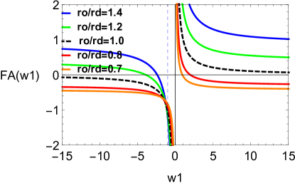
(a) With varying $r_{o}$

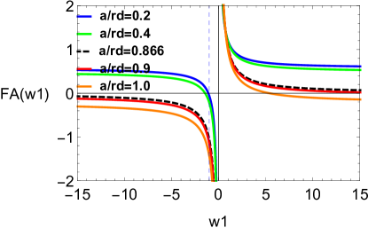
(b) With varying $a$

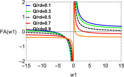
(c) With varying $Q$

Figure 3: (color online). Plots to show the flare-out condition satisfied by varying the parameters $r_{o}$, $a$, and $Q$ for the rotating wormhole.

Figure 3 represents some particular cases of the flare-out condition for the rotating wormhole. We use the vertical axis as Eq. (45), while the horizontal axis is $w_{1}$. The dashed blue line represents the location of $w_{1}=-1$. The dashed black hole line represents the case of location of $r^{2}_{o}=Q^{2}+a^{2}$, in which $r_{o}/r_{d}=1$, $Q/r_{d}=0.5$, and $a/r_{d}=0.866025$. The blue and green lines represent the cases satisfying Eq. (47), while the red and orange lines represent the case satisfying Eq. (48). Figure 3(a) shows the flare-out condition with varying $r_{o}$. We take $a/r_{d}=0.866025$ and $Q/r_{d}=0.5$. The blue curve represents $r_{o}/r_{d}=1.4$, green represents $r_{o}/r_{d}=1.2$, red represents $r_{o}/r_{d}=0.8$, and orange represents $r_{o}/r_{d}=0.7$. Figure 3(b) shows the flare-out condition with varying $a$. We take $r_{o}/r_{d}=1$ and $Q/r_{d}=0.5$. The blue curve represents $a/r_{d}=0.2$, green represents $a/r_{d}=0.4$, red represents $a/r_{d}=0.9$, and orange represents $a/r_{d}=1.0$. Figure 3(c) shows the flare-out condition with varying $Q$. We take $r_{o}/r_{d}=1$ and $a/r_{d}=0.866025$. The blue curve represents $Q/r_{d}=0.1$, green represents $Q/r_{d}=0.3$, red represents $Q/r_{d}=0.7$, and orange represents $Q/r_{d}=0.9$. Since the wormhole geometry satisfying the flare-out condition requires the $FA(w_{1})$ to be greater than zero, we obtain the constraint on the value of the equation of state parameters as Eqs. (47) and (48).

3.4 Maxwell field

In this section, we present the solutions to Maxwell equations. When a charged wormhole rotates, a magnetic field could be induced, and this induced magnetic field and complicated geometry by the rotation make it difficult to solve Maxwell equations directly to find the solutions [43, 41].

We have experience in finding the Maxwell field for the charged rotating black hole with a matter field [41]. We want to apply this method directly to find the Maxwell field for a charged rotating wormhole. When solving Maxwell equations (5), to remove the functional dependence of the $\sqrt{-\det g_{\mu\nu}}$ on the function $\sqrt{A(r,\theta)}$ shown in Eq. (38), we multiply the Maxwell field by $1/\sqrt{A(r,\theta)}$, which immediately satisfies Maxwell equations (5). They are as follows:

$$F^{tr} = -F^{rt}=\frac{1}{\sqrt{A(r,\theta)}}\frac{Q}{\rho^{6}}(r^{2}-a^{2}\cos^{2}\theta)(r^{2}+a^{2})\,,$$

$$F^{t\theta} = -F^{\theta t}=\frac{1}{\sqrt{A(r,\theta)}}\frac{Q}{\rho^{6}}(-a^{2}r\sin 2\theta)\,,$$

$$F^{r\phi} = -F^{\phi r}=\frac{1}{\sqrt{A(r,\theta)}}\frac{Q}{\rho^{6}}a(a^{2}\cos^{2}\theta-r^{2})\,,$$

$$F^{\theta\phi} = -F^{\phi\theta}=\frac{1}{\sqrt{A(r,\theta)}}\frac{Q}{\rho^{6}}2ar\cot\theta\,.$$ (49)

For the Kerr-Newman type rotating black hole, $F(r,\theta)=G(r,\theta)$ as shown in [41].

In the asymptotic rest frame with $r\gg a$, the non-vanishing electromagnetic fields with (41) takes the usual form

$$E^{\hat{r}} = F^{{\hat{t}}{\hat{r}}}\simeq\frac{Q}{r^{2}}\,,$$

$$B^{\hat{r}} = F^{{\hat{\theta}}{\hat{\phi}}}\simeq 2\frac{Qa}{r^{3}}\cos\theta\,,$$

$$B^{\hat{\theta}} = F^{{\hat{\phi}}{\hat{r}}}\simeq\frac{Qa}{r^{3}}\sin\theta\,.$$ (50)

The above are the induced dipole magnetic field and ${\cal M}=Qa$ corresponds to the magnetic moment of the wormhole. They are the same for the black hole up to the leading order [73].

4 Summary and discussions

We presented a new charged wormhole solution supported by anisotropic matter fields in an asymptotically flat spacetime. To achieve this, we first adopted a static spherically symmetric ansatz with a charge and displayed the solution to the Einstein-Maxwell equations. The anisotropic matter has two equations of state parameters. One, $w_{1}$, is given as a constant, while the other, $w_{2}$ is obtained as a function of $r$, along with that constant and the charge $Q$.

We, then, analyzed the conditions for our solutions to be a traversable wormhole geometry. While analyzing the metric functions, we have made a few observations about how it differs from the geometry of a black hole. First of all, the wormhole geometry does not have an event horizon and does not exhibit singularities in its geometry. We mentioned physical meanings of where the metric functions $f(r)$ and $g(r)$ vanishes. For the wormhole geometry, considering an asymptotically flat geometry, we obtained that the magnitude of the charge $Q$ is constrained to be smaller than the size of the wormhole throat. The condition on the asymptotically flat geometry for $w_{1}$ is the same as the condition on $w_{1}$ which gives a value to be the wormhole geometry that satisfies the flare-out condition. We also analyzed the exoticity function, which is directly related to the violation of the null energy condition. We also analyzed the magnitudes of tidal accelerations at the wormhole throat in the figure 2, in which we recovered the speed of light $c$, the gravitational constant $G$, and Coulomb’s constant $k$ in SI units. We showed the condition that the tidal effect is small enough so that a traveler through the wormhole would have stable travel.

Many objects rotate in the Universe, thus constructing a rotating wormhole geometry would be quite interesting. Teo first obtained a rotating wormhole geometry [49], and since then there have been a lot of studies on the rotating wormhole geometry [74, 50, 75, 76, 77, 52, 51, 78, 79, 53, 80, 81, 82, 54, 83]. To get a rotating version of our charged wormhole, we have employed the NJ algorithm. We introduced $a$ as a rotation parameter. The position of the throat of the rotating wormhole is dependent on an angular coordinate. We have analyzed the flare-out condition for this geometry to be a rotating wormhole. For this purpose, we checked a three-dimensional space with ${\rm t=constant}$, $\theta=\pi/2$ and $\theta=0$, and checked that the circumference radius has the diverging property at the throat of the wormhole. We leave the detailed analysis of the surplus angle for future work. We obtained the constraint on the charge $Q$ and the parameter $a$, which are smaller than the size of the throat separately, and obtained the constraint on the value of the equation of state parameters due to the rotation effect for $w_{1}<-1$. When $a^{2}+Q^{2}>r^{2}_{o}$, the wormhole geometries with only a small range of $w_{1}$ could satisfy both the flare-out condition and the condition on the asymptotically flat spacetime.

We chose the location of the wormhole throat to be $G(r,\theta)=0$ to ensure the smooth passing of the Maxwell fields at the throat. Although the metric functions in front of $d\phi^{2}$ and $dtd\phi$ diverge at the throat, but we do not expect this divergence to cause curvature singularities at the throat.

We could arrive at a successful close to obtaining solutions by looking at the shape of Maxwell equations. In this way, if the metric function is different from the case of a rotating black hole [42, 43, 45, 40], the different effect shows up in the Maxwell tensor. To get the electric field and induced magnetic field components in the asymptotic region, we obtained the tetrad basis vectors, and on those bases, we found the electric field and induced magnetic field. It was shown that the electric and induced magnetic fields in this asymptotic region are the same as in the case of the black hole up to the leading order [73].

When an electric field converges on a wormhole from one universe passes through the wormhole, and exits into the other universe. At the throat, the Maxwell tensor goes to zero. If one takes a Gaussian surface, which surrounds the asymptotic regions of both universes, there is the flux of an electric field coming out as there is going in, thus there exists no real charge within the Gaussian surface. We have shown solutions to the source-free Maxwell equations by constructing the wormhole geometry with charge $Q$, and we believe that this wormhole geometry provides the geometric realization corresponding to the concept of ‘charge without charge’ [36].

The topic of checking the stability of a wormhole would be interesting, and we will leave the study on this topic for future work [22, 86, 87, 88, 89].

References

- [1] A. Einstein, Annalen Phys. 49, no.7, 769-822 (1916).
- [2] B. P. Abbott et al. [LIGO Scientific and Virgo], Phys. Rev. Lett. 116, no.6, 061102 (2016) [arXiv:1602.03837 [gr-qc]].
- [3] B. P. Abbott et al. [LIGO Scientific and Virgo], Phys. Rev. Lett. 119, no.16, 161101 (2017) [arXiv:1710.05832 [gr-qc]].
- [4] K. Akiyama et al. [Event Horizon Telescope], Astrophys. J. Lett. 875, L1 (2019) [arXiv:1906.11238 [astro-ph.GA]].
- [5] K. Akiyama et al. [Event Horizon Telescope], Astrophys. J. Lett. 930, no.2, L12 (2022) [arXiv:2311.08680 [astro-ph.HE]].
- [6] M. S. Morris and K. S. Thorne, Am. J. Phys. 56, 395-412 (1988).
- [7] M. S. Morris, K. S. Thorne and U. Yurtsever, Phys. Rev. Lett. 61, 1446-1449 (1988).
- [8] J. R. Gott, III, Phys. Rev. Lett. 66, 1126-1129 (1991).
- [9] I. D. Novikov, Phys. Rev. D 45, 1989-1994 (1992).
- [10] B. Shoshany, SciPost Phys. Lect. Notes 10, 1 (2019) [arXiv:1907.04178 [gr-qc]].
- [11] O. James, E. von Tunzelmann, P. Franklin and K. S. Thorne, Am. J. Phys. 83, 486 (2015) [arXiv:1502.03809 [gr-qc]].
- [12] A. Einstein and N. Rosen, Phys. Rev. 48, 73-77 (1935).
- [13] M. Visser, Lorentzian wormholes: From Einstein to Hawking, AIP Press, New York, (1995).
- [14] F. S. N. Lobo, [arXiv:0710.4474 [gr-qc]].
- [15] S. W. Kim, Phys. Rev. D 53, 6889-6892 (1996).
- [16] S. W. Kim and S. P. Kim, Phys. Rev. D 58, 087703 (1998) [arXiv:gr-qc/9907012 [gr-qc]].
- [17] F. S. N. Lobo and M. A. Oliveira, Phys. Rev. D 80, 104012 (2009) [arXiv:0909.5539 [gr-qc]].
- [18] P. Kanti, B. Kleihaus and J. Kunz, Phys. Rev. Lett. 107, 271101 (2011) [arXiv:1108.3003 [gr-qc]].
- [19] J. Y. Kim and M. I. Park, Eur. Phys. J. C 76, no.11, 621 (2016) [arXiv:1608.00445 [hep-th]].
- [20] J. Maldacena, A. Milekhin and F. Popov, [arXiv:1807.04726 [hep-th]].
- [21] A. Övgün, K. Jusufi and İ. Sakallı, Phys. Rev. D 99, no.2, 024042 (2019) [arXiv:1804.09911 [gr-qc]].
- [22] Y. Kang and S. W. Kim, J. Korean Phys. Soc. 73, no.12, 1800-1807 (2018).
- [23] H. C. Kim and Y. Lee, [arXiv:1902.02957 [gr-qc]].
- [24] S. Halder, S. Bhattacharya and S. Chakraborty, Mod. Phys. Lett. A 34, no.12, 1950095 (2019) [arXiv:1903.11998 [gr-qc]].
- [25] M. Bouhmadi-López, C. Y. Chen, X. Y. Chew, Y. C. Ong and D. h. Yeom, JCAP 10, 059 (2021) [arXiv:2108.07302 [gr-qc]].
- [26] A. G. Agnese, A. P. Billyard, H. Liu and P. S. Wesson, Gen. Rel. Grav. 31, 527-535 (1999) [arXiv:gr-qc/9905037 [gr-qc]].
- [27] W. T. Kim, J. J. Oh and M. S. Yoon, Phys. Rev. D 70, 044006 (2004) [arXiv:gr-qc/0307034 [gr-qc]].
- [28] F. S. N. Lobo, Phys. Rev. D 75, 064027 (2007) [arXiv:gr-qc/0701133 [gr-qc]].
- [29] D. Bak, C. Kim and S. H. Yi, JHEP 08, 140 (2018) [arXiv:1805.12349 [hep-th]].
- [30] J. de Boer, V. Jahnke, K. Y. Kim and J. F. Pedraza, JHEP 05, 141 (2023) [arXiv:2211.13262 [hep-th]].
- [31] J. L. Blázquez-Salcedo, C. Knoll and E. Radu, Phys. Rev. Lett. 126, no.10, 101102 (2021) [arXiv:2010.07317 [gr-qc]].
- [32] R. A. Konoplya and A. Zhidenko, Phys. Rev. Lett. 128, no.9, 091104 (2022) [arXiv:2106.05034 [gr-qc]].
- [33] D. L. Danielson, G. Satishchandran, R. M. Wald and R. J. Weinbaum, Phys. Rev. D 104, no.12, 124055 (2021) [arXiv:2108.13361 [gr-qc]].
- [34] J. L. Blázquez-Salcedo, C. Knoll and E. Radu, Eur. Phys. J. C 82, no.6, 533 (2022) [arXiv:2108.12187 [gr-qc]].
- [35] F. S. N. Lobo, Phys. Rev. D 71, 084011 (2005) [arXiv:gr-qc/0502099 [gr-qc]].
- [36] C. W. Misner and J. A. Wheeler, Annals Phys. 2, 525-603 (1957).
- [37] S. W. Kim and H. Lee, Phys. Rev. D 63, 064014 (2001) [arXiv:gr-qc/0102077 [gr-qc]].
- [38] S. Halder, S. Bhattacharya and S. Chakraborty, Phys. Lett. B 791, 270-275 (2019) [arXiv:1903.03343 [gr-qc]].
- [39] H. C. Kim and Y. Lee, JCAP 09, 001 (2019) [arXiv:1905.10050 [gr-qc]].
- [40] H. C. Kim, B. H. Lee, W. Lee and Y. Lee, Phys. Rev. D 101, no.6, 064067 (2020) [arXiv:1912.09709 [gr-qc]].
- [41] H. C. Kim, B. H. Lee, W. Lee and Y. Lee, [arXiv:2112.04131 [gr-qc]].
- [42] R. P. Kerr, Phys. Rev. Lett. 11, 237-238 (1963).
- [43] E. T. Newman, R. Couch, K. Chinnapared, A. Exton, A. Prakash and R. Torrence, J. Math. Phys. 6, 918-919 (1965).
- [44] B. Carter, Les Houches Summer School of Theoretical Physics, 57-214, (1973).
- [45] B. Toshmatov, Z. Stuchlík and B. Ahmedov, Eur. Phys. J. Plus 132, no.2, 98 (2017) [arXiv:1512.01498 [gr-qc]].
- [46] Z. Xu and J. Wang, Phys. Rev. D 95, no.6, 064015 (2017) [arXiv:1609.02045 [gr-qc]].
- [47] E. T. Newman and A. I. Janis, J. Math. Phys. 6, 915-917 (1965).
- [48] M. Azreg-Aïnou, Phys. Rev. D 90, no.6, 064041 (2014) [arXiv:1405.2569 [gr-qc]].
- [49] E. Teo, Phys. Rev. D 58, 024014 (1998) [arXiv:gr-qc/9803098 [gr-qc]].
- [50] P. K. F. Kuhfittig, Phys. Rev. D 67, 064015 (2003) [arXiv:gr-qc/0401028 [gr-qc]].
- [51] M. Azreg-Aïnou, Eur. Phys. J. C 74, no.5, 2865 (2014) [arXiv:1401.4292 [gr-qc]].
- [52] B. Kleihaus and J. Kunz, Phys. Rev. D 90, 121503 (2014) [arXiv:1409.1503 [gr-qc]].
- [53] X. Y. Chew, B. Kleihaus and J. Kunz, Phys. Rev. D 97, no.6, 064026 (2018) [arXiv:1802.00365 [gr-qc]].
- [54] G. Clément and D. Gal’tsov, Phys. Lett. B 838, 137677 (2023) [arXiv:2210.08913 [gr-qc]].
- [55] G. W. Gibbons and S. W. Hawking, Phys. Rev. D 15, 2752-2756 (1977).
- [56] S. W. Hawking and S. F. Ross, Phys. Rev. D 52, 5865-5876 (1995) [arXiv:hep-th/9504019 [hep-th]].
- [57] K. Schwarzschild, Sitzungsber. Preuss. Akad. Wiss. Berlin (Math. Phys. ) 1916, 189-196 (1916) [arXiv:physics/9905030 [physics]].
- [58] H. Reissner, Annalen Phys. 355, no.9, 106-120 (1916).
- [59] F. R. Tangherlini, Nuovo Cim. 27, 636-651 (1963).
- [60] V. V. Kiselev, Class. Quant. Grav. 20, 1187-1198 (2003) [arXiv:gr-qc/0210040 [gr-qc]].
- [61] S. A. Hayward, Phys. Rev. Lett. 96, 031103 (2006) [arXiv:gr-qc/0506126 [gr-qc]].
- [62] I. Cho and H. C. Kim, Chin. Phys. C 43, no.2, 025101 (2019) [arXiv:1703.01103 [gr-qc]].
- [63] S. Jeong, B. H. Lee, H. Lee and W. Lee, Phys. Rev. D 107, no.10, 104037 (2023) [arXiv:2301.12198 [gr-qc]].
- [64] T. Jacobson, Class. Quant. Grav. 24, 5717-5719 (2007) [arXiv:0707.3222 [gr-qc]].
- [65] R. Penrose, Phys. Rev. Lett. 14, 57-59 (1965).
- [66] A. Ashtekar and B. Krishnan, Living Rev. Rel. 7, 10 (2004) [arXiv:gr-qc/0407042 [gr-qc]].
- [67] J. M. M. Senovilla, Int. J. Mod. Phys. D 20, 2139 (2011) [arXiv:1107.1344 [gr-qc]].
- [68] D. Hochberg and M. Visser, Phys. Rev. D 58, 044021 (1998) [arXiv:gr-qc/9802046 [gr-qc]].
- [69] K. Raviteja and S. Gutti, Phys. Rev. D 102, no.2, 024072 (2020) [arXiv:2006.06468 [gr-qc]].
- [70] D. Hochberg and M. Visser, Phys. Rev. D 56, 4745-4755 (1997) [arXiv:gr-qc/9704082 [gr-qc]].
- [71] S. W. Kim, J. Korean Phys. Soc. 63, 1887-1891 (2013) [arXiv:1302.3337 [gr-qc]].
- [72] R. Shaikh and S. Kar, Phys. Rev. D 94, no.2, 024011 (2016) [arXiv:1604.02857 [gr-qc]].
- [73] C. W. Misner, K. S. Thorne and J. A. Wheeler, W. H. Freeman, 1973, 1279p.
- [74] V. M. Khatsymovsky, Phys. Lett. B 429, 254-262 (1998) [arXiv:gr-qc/9803027 [gr-qc]].
- [75] S. W. Kim, Nuovo Cim. B 120, 1235-1242 (2005) [arXiv:gr-qc/0401036 [gr-qc]].
- [76] P. E. Kashargin and S. V. Sushkov, Grav. Cosmol. 14, 80-85 (2008) [arXiv:0710.5656 [gr-qc]].
- [77] K. A. Bronnikov, V. G. Krechet and J. P. S. Lemos, Phys. Rev. D 87, 084060 (2013) [arXiv:1303.2993 [gr-qc]].
- [78] J. C. Del Águila, T. Matos and G. Miranda, Phys. Rev. D 99, no.12, 124045 (2019) [arXiv:1507.02348 [gr-qc]].
- [79] X. Y. Chew, B. Kleihaus and J. Kunz, Phys. Rev. D 94, no.10, 104031 (2016) [arXiv:1608.05253 [gr-qc]].
- [80] X. Y. Chew, V. Dzhunushaliev, V. Folomeev, B. Kleihaus and J. Kunz, Phys. Rev. D 100, no.4, 044019 (2019) [arXiv:1906.08742 [gr-qc]].
- [81] M. Azreg-Aïnou, Phys. Dark Univ. 32, 100802 (2021) [arXiv:2012.03431 [gr-qc]].
- [82] F. Rahaman, K. N. Singh, R. Shaikh, T. Manna and S. Aktar, Class. Quant. Grav. 38, no.21, 215007 (2021) [arXiv:2108.09930 [gr-qc]].
- [83] A. Cisterna, K. Müller, K. Pallikaris and A. Viganò, Phys. Rev. D 108, no.2, 024066 (2023) [arXiv:2306.14541 [gr-qc]].
- [84] A. I. Janis and E. T. Newman, J. Math. Phys. 6, 902-914 (1965).
- [85] H. Stephani, D. Kramer, M. A. H. MacCallum, C. Hoenselaers and E. Herlt, Exact solutions of Einstein’s field equations, Cambridge Univ. Press, Cambridge (2003).
- [86] J. Y. Kim, C. O. Lee and M. I. Park, Eur. Phys. J. C 78, no.12, 990 (2018) [arXiv:1808.03748 [hep-th]].
- [87] Y. Kang and S. W. Kim, Class. Quant. Grav. 37, no.10, 105012 (2020) [arXiv:1910.07715 [gr-qc]].
- [88] C. Jonas, G. Lavrelashvili and J. L. Lehners, Phys. Rev. D 109, no.8, 086022 (2024) [arXiv:2312.08971 [hep-th]].
- [89] B. H. Lee, W. Lee and Y. H. Qi, [arXiv:2311.10559 [gr-qc]].