Shinsuke Iwao,
Kohei Motegi,
and Ryo Ohkawa
Email address: iwao-s@keio.jp
Faculty of Business and Commerce, Keio University,Hiyosi 4–1–1, Kohoku-ku, Yokohama-si, Kanagawa 223-8521, Japan,
E-mail: kmoteg0@kaiyodai.ac.jp
Faculty of Marine Technology, Tokyo University of Marine Science and Technology,Etchujima 2-1-6, Koto-Ku, Tokyo, 135-8533, Japan,
E-mail: ohkawa.ryo@gmail.com, ohkawa.ryo@omu.ac.jp
Osaka Central Advanced Mathematical Institute, Osaka Metropolitan
University, 558-8585, Osaka, Japan,
Research Institute for Mathematical Sciences, Kyoto University,
606-8502, Kyoto, Japan.
Abstract
The tetrahedron equation introduced by Zamolodchikov is a three-dimensional generalization of the Yang-Baxter equation.
Several types of solutions to the tetrahedron equation that have connections to quantum groups can be viewed as -oscillator valued vertex models with matrix elements of the -operators given by generators of the -oscillator algebra acting on the Fock space.
Using one of the -oscillator valued vertex models introduced by Bazhanov-Sergeev, we introduce a family of partition functions that admits an explicit algebraic presentation using Schur functions.
Our construction is based on the three-dimensional realization of the Zamolodchikov-Faddeev algebra provided by Kuniba-Okado-Maruyama. Furthermore, we investigate an inhomogeneous generalization of the three-dimensional lattice model. We show that the inhomogeneous analog of (a certain subclass of) partition functions can be expressed as loop elementary symmetric functions.
1 Introduction
In [32, 33], Zamolodchikov introduced the tetrahedron equation as a three-dimensional generalization of the Yang-Baxter equation [1, 31].
Various seminal works such as [2, 3, 6, 13, 14, 16] have been done
to construct solutions to the tetrahedron equation.
See [4, 5, 17, 18, 19, 21, 24], as well as more recently [20], for examples of studies that investigate solutions to the tetrahedron equation through the viewpoint of quantum groups [8, 9, 10, 12].
Solutions to the tetrahedron equation which we call as three-dimensional -matrices are regarded as “local Boltzmann weights” in three-dimensional statistical physics.
In this paper, we study a class of partition functions
using one of the solutions found by Bazhanov-Sergeev [5], where
they used the three-dimensional -matrix and gave an unconventional realization of the -matrix by tracing out one dimension.
Our main idea is to use a degeneration of the three-dimensional -matrix,
which was studied by Kuniba-Maruyama-Okado [18, 19] from the perspective of its relation to a multispecies generalization of a totally asymmetric symmetric exclusion process (TASEP) [7, 29].
They showed that the matrix product form of the steady state of the multispecies periodic TASEP introduced by Ferrari-Martin [11] can be transformed into a certain type of partition functions constructed from Bazhanov-Sergeev’s three-dimensional -matrix.
This result was given by bypassing the crystal basis theory [15, 26].
Furthermore,
they showed that layers of the three-dimensional partition functions
satisfy the Zamolodchikov-Faddeev algebra relations, i.e.
they gave a realization of generators of the (degenerated) Zamolodchikov-Faddeev algebra.
The partition functions corresponding to the steady state were constructed by taking the traces of the product of the Zamolodchikov-Faddeev operators acting on the tensor product of Fock spaces and specializing spectral parameters to a specific value.
In this paper, we study a closely related but different class of three-dimensional partition functions.
Instead of taking the traces, our partition functions are given by taking the vacuum expectation values of the Zamolodchikov-Faddeev operators.
In addition, we do not specialize spectral parameters to a specific value, as they will play the role of symmetric variables.
We show that this class of partition functions is represented as Schur polynomials up to an overall factor.
This result is derived from multiple commutation relations of the Zamolodchikov-Faddeev algebra.
Furthermore, we also investigate an inhomogeneous generalization.
Since this generalization does not respect integrability, techniques based on integrable systems such as the
Zamolodchikov-Faddeev algebra cannot be applicable here.
However, we show that a certain subclass of inhomogeneous partition functions can be expressed as loop elementary symmetric functions, which was originally introduced by Yamada [30] in the context of the discrete Toda lattice.
See Lam-Pylyavskyy [22, 23] for more details.
We also show that several other partition functions are given by loop elementary symmetric functions.
This paper is organized as follows.
Section 2 first reviews some basic facts about the three-dimensional -matrix and its equivalent description as an operator-valued two-dimensional -matrix.
We next recall a realization of the Zamolodchikov-Faddeev operators, and introduce partition functions.
We derive the correspondence with the Schur functions in Section 3 and also discuss some corollaries/applications.
In section 4, we introduce an inhomogeneous version
for a subclass and several other related partition functions,
and prove the correspondence with the loop elementary symmetric functions.
2 Three-dimensional -matrix and partition functions
We first recall the three-dimensional -matrix [5, 18, 19]
and operators that are used in this paper,
and introduce the partition functions which we investigate.
Let be the complex two-dimensional space spanned by the standard basis , and let
be the bosonic Fock space spanned by the basis .
We introduce the linear operators acting on as
(2.1)
Here, .
These operators satisfy the relations
(2.2)
We refer to as the zero-number projection operator, the creation operator, and the annihilation operator, respectively.
The bosonic Fock space and the algebra associated can be regarded as the limit of the -bosonic Fock space
and the -oscillator algebra.
Let denote the dual space of , which is spanned by such that .
The dual Fock space is the vector space spanned by such that , where is the standard pairing.
The three-dimensional -matrix acting on
is defined by acting on the basis as
(2.3)
where
(2.4)
(2.5)
and otherwise.
This is equivalent to the operator-valued two-dimensional -operator acting on
as
(2.6)
where
(2.7)
(2.8)
and otherwise.
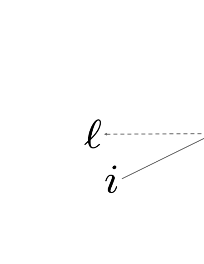
Figure 1: Three-dimensional -matrix. The two solid lines represent two two-dimensional spaces,
and the dashed line represents the bosonic Fock space.
To this configuration,
the ”Boltzmann weight” is assigned.
One can also regard this is as an ”operator-valued Boltzmann weight”
if not specifying the basis in the bosonic Fock space.
Figure 1 presents a graphical description of the three-dimensional -matrix in (2.3) (or equivalently, the operator-valued two-dimensional -matrix in (2.6)), which we use in this paper.
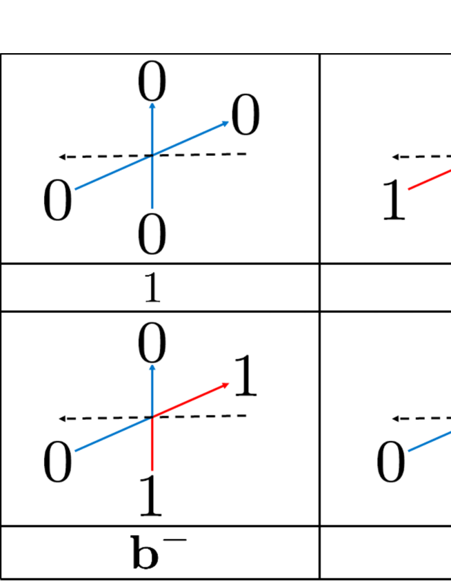
The matrix elements of are shown in Figure 2.
Let be the three-dimensional lattice spanned by the standard basis .
An element is often identified with the vector .
We will refer to the planes
,
, and
as
the -th row, the -th column, and the -th slice, respectively.
Let be the set consisting of points.
We assign a copy of the Fock space to each line for .
Hereinafter, denotes the Fock space assigned to .
Figure 2: The operator-valued matrix elements of .
We color the half-edges which are connected to 1s in the two-dimensional vector spaces with
red, and color 0s with
blue.
We denote the basis of
by .
The standard bases of
and its dual are given by
and
, respectively.
We introduce notations for the vacuum state and its dual as
and
.
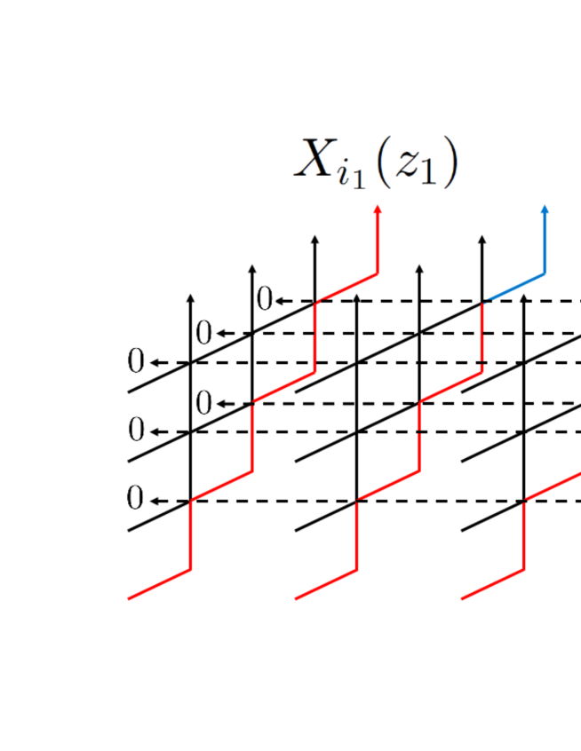
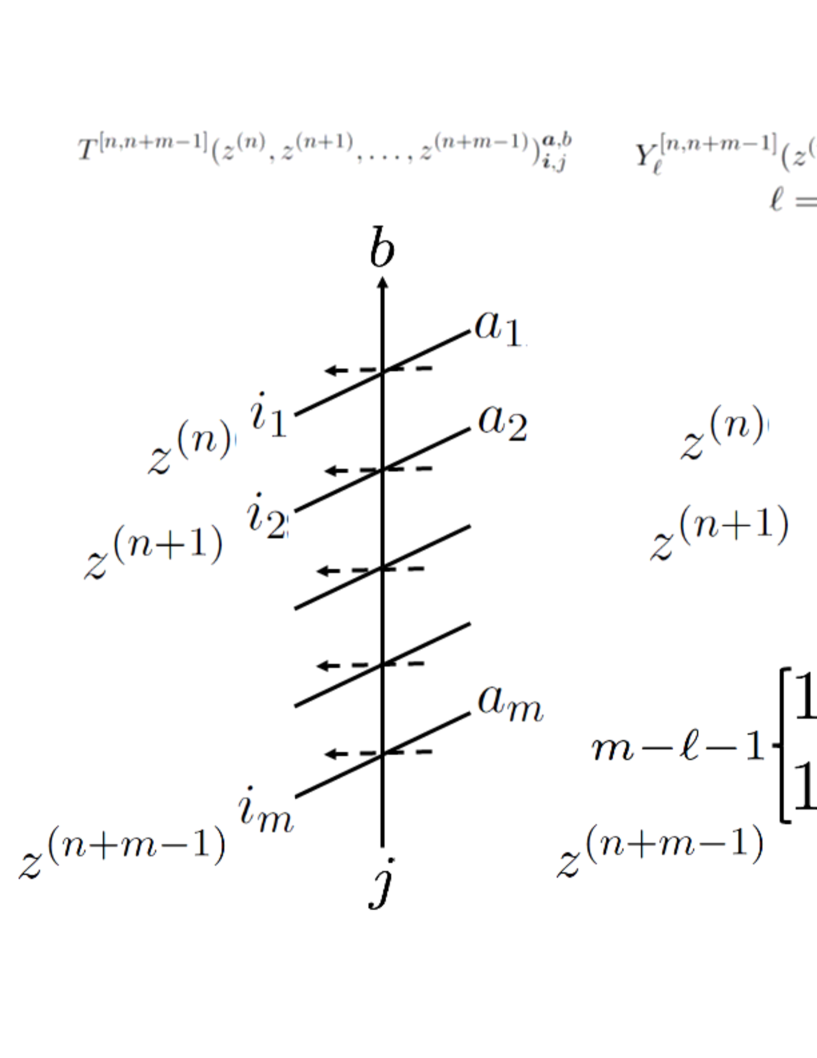
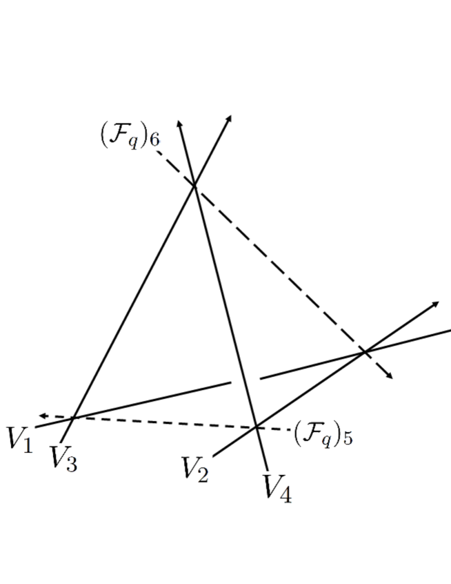
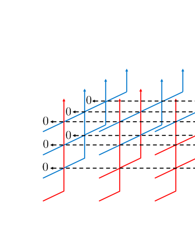
We introduce the linear operator [17, 18, 19] acting on the tensor space , which is graphically represented as Figure 3. Here, to each of intersections,
a matrix element of is assigned, which is determined according to the configuration of the red and blue segments.
is a weighted sum (see Figure 3) of all matrix elements of determined according to the possible configuration in which (i) the segments at the bottom of -th columns are colored by red, and
(ii) the segments at the bottom of -th columns are colored by blue.
Graphically, the operator sends a vector in to the next slice.
We will abbreviate as if there is no confusion.
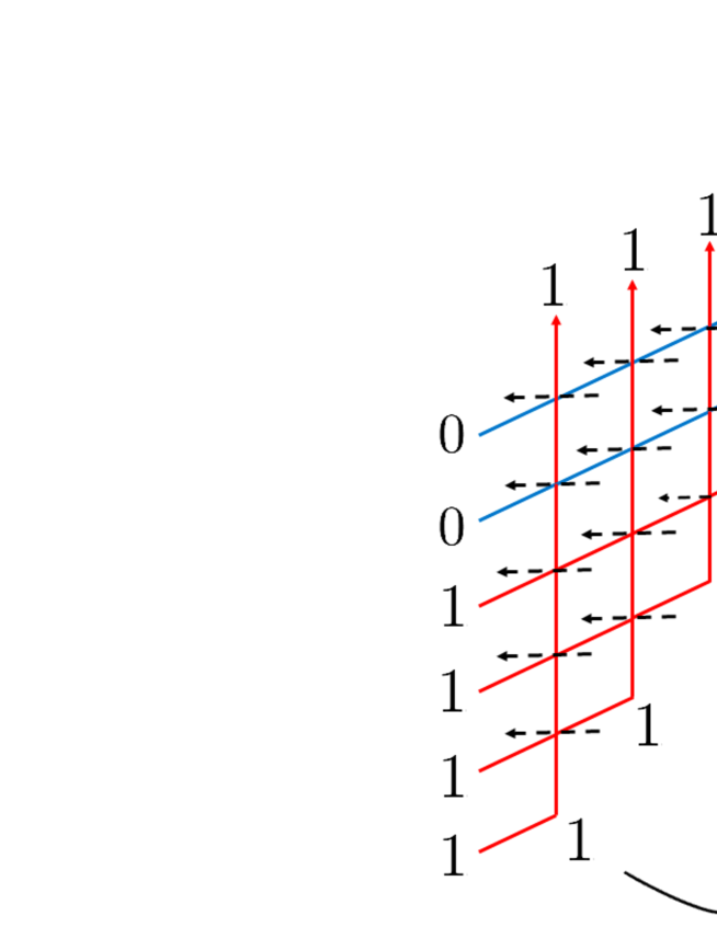
Figure 3: The operator .
We take the sum over all configurations except one side of the boundary
is fixed. The fixed boundary condition on one side is labeled by the subscript of the operator,
which corresponds to the number of consecutive number of integers which is fixed as
on the fixed boundary. The sum is weighted, and the power of
is the number of s at the top boundary.
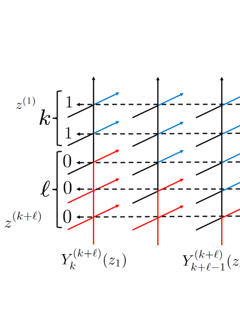
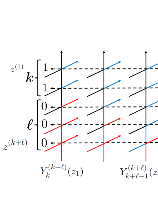
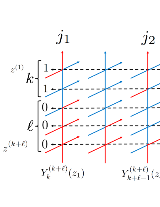
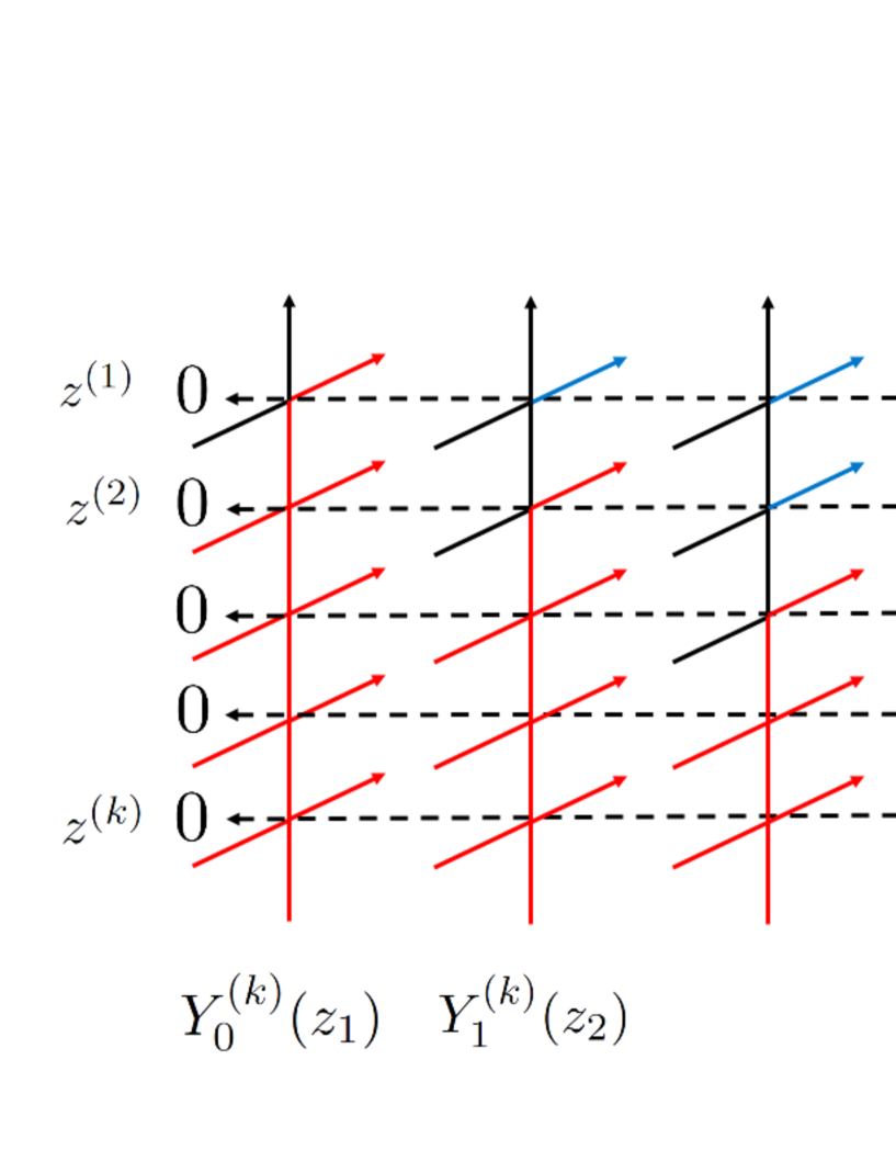
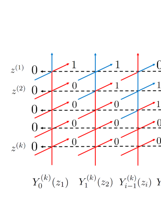
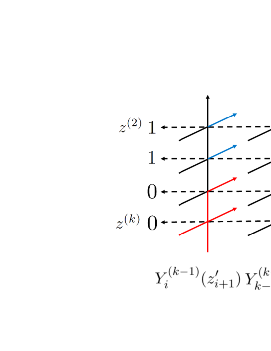
In this paper, we investigate the following three-dimensional partition function
Figure 4: The three-dimensional partition functions
.
We mainly investigate the case in this paper.
3 Three-dimensional partition functions and Schur functions
In this section, we study the partition function (2.9).
Let be the set of all possible configurations of the red and blue segments that fit Figure 3.
We expand as
(3.1)
where is the number of s in the topmost row in and
.
Then, is either , , , or .
We sometimes use the notation (resp. ) if and it arises from two blue (resp. red) lines crossing at .
The following is an immediate consequence of Figure 2.
Lemma 3.1.
We have the following:
1.
If and , then or .
2.
If and , then or .
3.
If and , then .
4.
If and , then .
We first show the following factorized expression
for cases .
Lemma 3.2.
When ,
we have
(3.2)
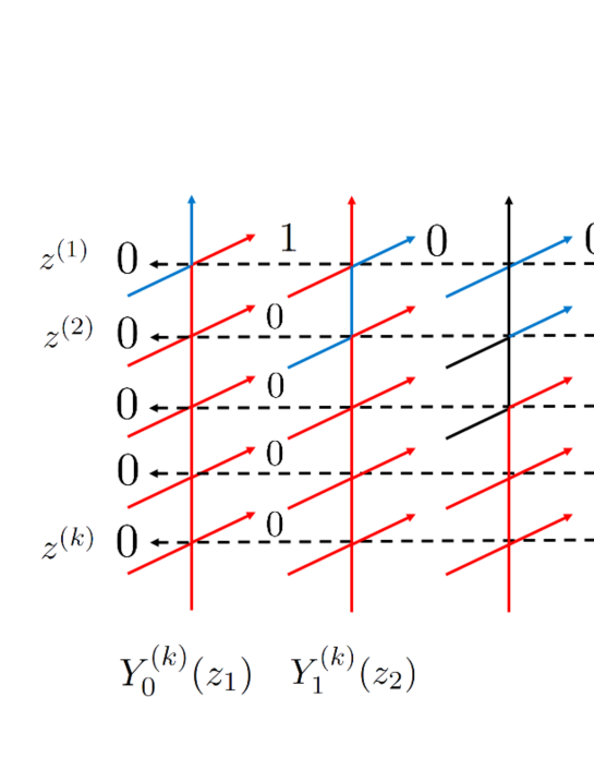
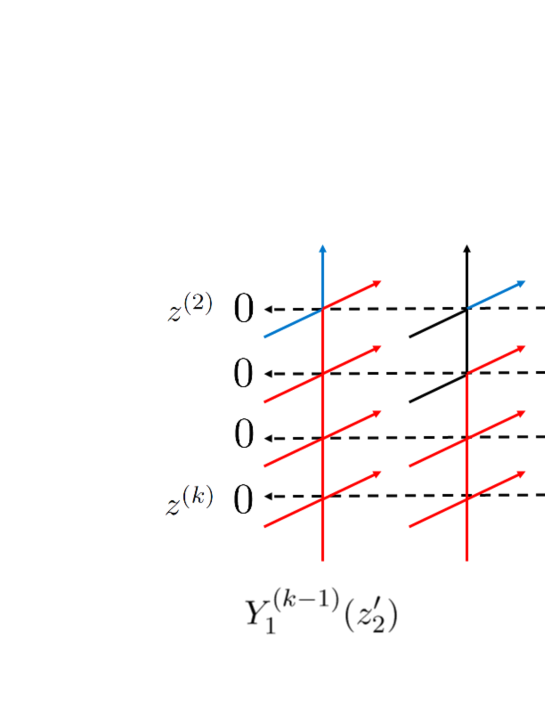
Proof.
We prove the lemma
by showing that there is only one
configuration that contributes to (3.2).
This can be checked by investigating the bosonic Fock spaces assigned to
.
We first see what happens to the Fock space .
Let .
Let denote the number of such that .
We let denote the sum .
In a similar manner, we define , , and .
By definition of , the component of each term in must be or .
From Figure 2, we also find that the component of a term in is , and that in is or .
Hence, the component of each term in should be a sequence of the form such that and .
However, since and , terms that can survive should satisfy and for all .
By the same reason, the components of terms in that can survive should be of the form .
Therefore, from Lemma 3.1, we find that the components of the survived terms are of the form .
For the same reason we previously noted, terms that can survive should be of the form .
We can repeat this procedure and show that the components of terms that can survive should be of the form .
Therefore, all the possible configurations at each intersection must consist of (i) two blue lines, (ii) two red lines, or (iii) one vertical red line and one horizontal blue line.
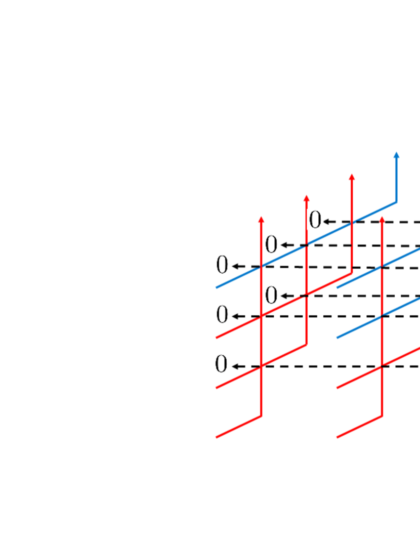
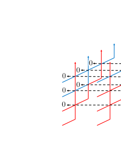
Figure 5 presents the only possible configuration on a slice corresponding to , the contribution of which is .
Multiplying these factors gives (3.2).
∎
Figure 5: The unique configuration for the operator in
when .
One notes from this configuration that from the factor contributes.
The operators
are shown to satisfy the following relations.
Theorem 3.3.
[17, 19]
The operators satisfy the Zamolodchikov-Faddeev algebra relations
(3.6)
Theorem 3.3 is proved in [17, 19] as a consequence
of the tetrahedron equation
(see Appendix A for the tetrahedron equation).
Recall the Schur polynomials.
For a sequence of integers
where
,
the Schur polynomials is
(3.7)
Let us introduce several shorthand notations.
For a set of variables
denote .
Note that due to commutativity , the ordering of variables in the product
does not matter. For an arbitrary integer ,
define .
We also introduce the following notations ,
for two sets of variables .
We use the following formula for Schur functions
( case of [27], Proposition 4).
Here, we take the sum over all
such that
are unordered sets of variables satisfying
and
.
We prepare the following multiple commutation relations
between the operators .
Proposition 3.5.
For ,
we have the following commutation relations:
(3.9)
Here, we take the sum over all
such that
are unordered sets of variables satisfying
and
.
Proof.
We can give a proof using the argument given in [25, 28].
We rewrite the Zamolodchikov-Faddeev algebra relations (3.3)
in the following forms
(3.10)
(3.11)
(3.12)
From these commutation relations, one notes there exist commutation relations
of the following form
(3.13)
and the problem is to determine explicitly.
Fix
and first note that the left hand side of (3.13)
can be rewritten using (3.11), (3.12) as
(3.14)
Next, we reverse the order of the operators in
the right hand side of (3.14)
using (3.10).
We note that to get the term
in this way,
we only need to keep track of the first term of the right hand side of (3.10),
and we get the factor .
Hence we find is
(3.15)
These coefficients are uniquley determined by
Lemma 3.2.
∎
Using Lemma 3.2,
Proposition 3.4, Proposition 3.5,
we determine the explicit forms of the partition functions.
Theorem 3.6.
For , we have
(3.16)
In particular, the simplest case gives the following.
Theorem 3.7.
For , we have
(3.17)
Proof.
From (3.9),
we have the following relation between partition functions
Let us see some examples. Consider the case , ,
.
From (3.17), we have
(3.24)
where
is the elementary symmetric functions
.
Using
(3.25)
we have
(3.26)
More generally, first
recall the Jacobi-Trudi formula for the Schur functions
(3.27)
where is the conjugate partition of ,
and
is the length of .
Using (3.17), (3.25),
(3.27) and the property of differential operators
acting on determinants, we have
(3.28)
Hence we get
(3.29)
Let us also see the case when the variables are all specialized to 1.
Recall the factorization of Schur polynomials when specializing the variables
(3.30)
which is well-known, which follows from the determinant form for example.
Applying this factorization to (3.17), we have the following.
Corollary 3.9.
For , we have
(3.31)
This corollary corresponds to counting the number of configurations
contributing to the partition functions.
Let us finally discuss an
application/interpretation of this result to
probability theory/statistical physics.
The shape for the partition functions
which we consider can be viewed as a prism
with two bases which are triangles and three lateral faces
which are rectangles.
To each of the lateral faces, there are points associated,
each point
colored with either red or blue.
To each edge of the triangles corresponding to bases,
there are points associated,
each of which is colored with red or blue.
The following quantity
(3.34)
corresponds to the average number of points lying on one edge of the base is colored with red, under the boundary condition
such that coloring on points on
one of the lateral faces is fixed which can be labelled by
,
and the boundaries corresponding to the other two lateral faces
are free.
(3.33) means that for the case
when the fixed boundary is labelled by
,
the average number of points on one edge
of the base
colored with red is .
4 Inhomogeneous three-dimensional partition functions and loop elementary symmetric functions
Figure 6: The operator-valued matrix elements of .
and in is replaced by
and .
This section discusses an inhomogeneous generalization
of the partition function.
We derive explicit representations for one of the simplest cases
by brute force computation.
We use the following three-dimensional -operator , which is a degeneration of the one in [5] (see [17], (18.23) for example)
Let be a set of independent variables.
Each is associated with the line .
We define the linear operator , which acts on , as the sum of matrix elements of
over all possible configurations that we mentioned in Section 2.
See Figure 7.
Although depends on several variables
,
we keep to use .
Hereinafter, we refer to such as a multiple variable.
When for all ,
reduces to .
Figure 7: The operator .
We use in the -th row and -th column .
For a string of multiple variables, we define the operator
.
For strings of multiple variables , , we consider the partition function
(4.4)
Let denote the number of elements of .
Note the operator
depends on variables
in principle. However, as shown in the theorem below,
the partition functions
(4.4)
which is sandwiched by the vacuum state and its dual
actually depend on fewer variables.
Theorem 4.1.
Assume for all .
Let , ,
, and .
Then, we have
(4.5)
where is the concatenation of the strings: .
In particular, when , we have , and
This polynomial is a special case of loop elementary symmetric functions
[22, 23, 30].
Since the notations become complicated and can be proved in the same way
for the general case,
we show the following case corresponding to
.
Theorem 4.2.
We have
(4.6)
Figure 8:
One-column operators
(left), (middle) and (right).
Before proving Theorem 4.2, let us introduce several notations.
Let be a multiple variable.
For brevity, we write .
For two sets of indices and , we introduce the linear operator
(4.7)
which acts on .
We also introduce the following operators
which are certain sums of the operators which we have just introduced
(4.8)
for
and
(4.9)
Graphical descriptions of these operators are given
in Figure 8.
If there is no confusion, we use the abbreviations
Let
We also introduce the following notations for (dual) vectors
(4.10)
(4.11)
Figure 9: The operator in
the inhomogeneous partition functions
.
We find
the -operators from the second to the -th columns are all fixed,
and the -operators in the first column form the operator
.
Lemma 4.3.
For a non-negative integer, we have
(4.12)
Proof.
This can be shown in
a similar manner to the proof of
Lemma 3.2.
Let .
By investigating the bosonic Fock spaces ,
,
we find that configurations that survive in should satisfy the following property:
On the slice that corresponds to , the matrix element assigned to is (i) if , and (ii) if and .
(Figure 9 presents a such configuration.)
This fact implies that can
be factorized as a product
of the partition function constructed only from the first column
and that constructed from the other columns.
Since the latter becomes , is equal to the one constructed from the first column,
i.e. we note that the three-dimensional partition functions are reduced to
partition functions
(4.13)
consisting only of -operators in
the first column, i.e., operators ,
sandwiched by reduced (dual) vacuum vectors ,
which are reductions of the original vacuum vectors .
∎
Figure 10:
Another class of partition functions
constructed from one-row operators
.
From Lemma 4.3,
the proof of Theorem 4.2
reduces to showing that
the right-hand side of (4.12)
is given by the loop elementary symmetric function (4.6).
For this, we prepare the following Lemma 4.4 about
some special type of
partition functions constructed from one-column operators
(Figure 10)
and loop elementary symmetric functions.
Figure 11: Configurations which contribute to the partition functions.
Investigating the edges connecting the last two dashed lines
(with which and are associated)
which were not colored in Figure 10,
we find only one of the edges is colored with red,
and the others are colored with blue.
We also note that starting from that red edge,
there is a straight red line passing through that column,
and the columns right to that column are all colored with blue (top panel).
Repeating this argument, we find every nontrivial configuration
can be graphically represented as the bottom panel.
Lemma 4.4.
For and , we have
(4.14)
Proof.
We present a proof based on a graphical representation.
See
Figure 10.
First, we observe that from the -th to the -th columns,
only one of the edges with which and are associated
connecting the last two dashed lines
is colored with red, and the rest are colored with blue.
One can observe this as follows.
In the bottom layer,
one can see from Figure 10
that
there can be at most one annihilation
operator
coming from the -th column.
If there is no annihilation operator,
then the edges in the -th column are colored with red,
and the edges in the -th columns are colored with blue since the operators are sandwiched by
and and
neither creation nor annihilation operators can appear.
When there is one annihilation operator arising
from the -th column,
there must be exactly one annihilation operator
arsing from one of the -th columns
which the uncolored edges must be colored with red,
and the other columns corresponding to identity operators
must be colored with blue.
Next, we note that colors of edges in the column
layer which contains the red-colored connecting edge
are uniquely determined, and then note all colors
in the column layers right to that layer
are determined to be blue (Figure 11, top).
Let us see this in some more detail.
When looking the -th row of the column
layer which contains the red-colored connecting edge,
we note the operator-valued -operator assigned
has the form .
In this case, for this to be nonzero, and
must be , . One can continue this observation,
and we find there is a red line passing through the column,
and zero-number projection operators arise from the
first to the -th row.
From this, we note the edges in the column layers right to that layer are all colored with blue.
This can be understood in the same way.
When looking the -th row of those column
layers,
we note every operator-valued -operator assigned
has the form .
For this to be nonzero,
either which corresponds to the identity operator
or which corresponds to the creation operator.
However, since we have to multiply by the zero-number projection operators after all, using
case does not contribute
to the partition function, and one gets .
One can repeat this argument
and find all edges in those layers
are colored with blue.
Repeating the argument above, we find that all admissible
configurations can be represented as Figure 11, bottom.
There are red lines
partially passing through the column, which
can be labelled by integers .
Let us denote the contribution to the partition function
coming from this configuration as .
Computing the products of weights for this configuration,
we find
(4.15)
Taking all configurations into account,
i.e. taking sum
gives the explicit expression of the partition function
(4.14).
∎
Finally, we show the partition functions
given in Figure 12
give loop elementary functions.
Figure 12:
Partition functions
constructed from one-column operators.
Proposition 4.5.
We have
(4.16)
Proof.
We prove by induction on
with the help of Lemma 4.4.
Suppose (4.16) with replaced by holds.
For , consider the projection operator
which sends to
.
Then the identity operator decomposes into
(4.17)
By using (4.17), we decompose the left-hand side of (4.16)
as
(4.18)
Note that here we use the fact that one can further restrict the summands of the identity
operator (4.17) only to
and .
This is because in the top slice,
only the first column can produce an annihilation operator
(see Figure 12), and all the operators
coming from the first row
are finally sandwiched
by and ,
which means do not appear
since we cannot change to by acting
just one annihilation operator,
and we can neglect .
We first examine the first term in (4.18).
One can see the following relations hold
(4.19)
and
(4.20)
Here, .
One can apply the inductive assumption to
the right hand side of (4.20), which is
(4.21)
hence combining with
(4.19) and
(4.20), we find the first term of the left hand side of (4.18)
is (4.21).
Figure 13: The first term in (4.18)
is the case when 1 appears in the leftmost inner part
in the top dashed line.
After coloring parts in the solid lines which are already fixed to be red or blue,
we get the top panel.
We can remove the leftmost column layer as everything is fixed.
We can also remove the top row layer as the matrix elements of the -operators from the third to the last columns are all identity operators.
Removing the leftmost column and the top row layers,
we get the bottom panel, which is nothing but (4.21).
Figure 13
gives a graphical understanding of
the computations above to get (4.21).
Next we deal with the summands in (4.18).
Let us see the summands in the first sum.
One can show the first factor is
(4.22)
Acting the second factor on ,
we get
(4.23)
One can repeat this computation. Using
(4.24)
(4.25)
we get
(4.26)
Next we note that
(4.27)
Applying (4.14) in Lemma 4.4 to the right hand side of
(4.27), we get
(4.28)
Together with (4.26) and (4.27),
the first sum of the left hand side of (4.18) is given by
(4.29)
Figure 14: A summand of the first sum in (4.18)
is graphically represented as the top panel
after coloring parts in the solid lines which are already fixed to be red or blue.
Removing the leftmost column and the top row layers,
we get the bottom panel,
which corresponds to (4.28).
The removed parts contribute the factor
.
Multiplying with (4.28) gives
(4.29).
See
Figure 14
for a graphical derivation of (4.29).
In the same way, we can prove that
the second sum of the left hand side of (4.18) is given by
(4.30)
Finally, we note that the sum of
(4.21),
(4.29) and (4.30) can be written as
Combining Lemma 4.3
and Proposition
4.5,
we get Theorem 4.2.
Acknowledgement
S.I.
is supported by Grant-in-Aid for Scientific Research
19K03605, 22K03239, 23K03056, JSPS.
K.M.
is supported by Grant-in-Aid for Scientific Research 21K03176, 20K03793, JSPS.
R.O. is
supported by Grant-in-Aid for Scientific Research 21K03180, JSPS.
Appendix A: Tetrahedron equation
Figure 15:
Tetrahedron equation.
The left and right figure represents
and
respectively.
We record the tetrahedron equation and the original
three-dimensional -matrix for completeness.
See [5, 17, 19] for more details.
(4.1) is the degeneration of
the following version
where
and otherwise.
Here, , , ,
together with form the -Oscillator algebra
whose defining relations are
The operators act on
the basis of
-bosonic Fock space as
Define also
.
and can be viewed as operators acting on .
We can naturally extend this to operators acting on the tensor product
of many more two-dimensional and Fock spaces
by acting on three spaces nontrivially and the other spaces as identity.
It is customary to indicate the three spaces as subscripts.
and
imply they act on , and nontrivially
and the other spaces as identity.
Using these notations, the operators
satisfy the following tetrahedron equation (Figure
15)
[5, 17, 19]
where .
Both hand sides act on .
The Zamolodchikov-Faddeev algebra commutation relations
(3.3) are derived by using
the tetrahedron equation
[17, 19].
The degeneration of
in this Appendix gives the one used in section 4.
Note
.
Appendix B: Figures of configurations
We give several figures
in this appendix.
Figure 16
is an example of Lemma 3.2 which
corresponds to the case
.
The figure is the unique configuration.
The layer corresponding to
,
,
,
and
contributes the weight , ,
, and respectively,
and multiplying them gives .
Figure 16:
The unique nontrivial configuration for
.
The layer corresponding to
,
,
,
and
contributes the weight , ,
, and respectively,
and multiplying them gives .
Figure
17
gives an example of checking Theorem 3.6
which corresponds to the case
. There are three nontrivial configurations,
and each of them contributes the weight
,
and respectively.
Taking sum of the weights gives
.
Figure 17:
Three nontrivial
configurations for .
Configuration in top left, top right and bottom panel
contributes the weight
,
and respectively,
and taking sum gives .
References
[1]
R. J. Baxter,
Partition function for the eight-vertex lattice model,
Ann. Phys. 70, 193–-228 (1972).
[2]
R. J. Baxter,
On Zamolodchikov’s Solution of the Tetrahedron Equations,
Commun. Math. Phys. 88, 185–205 (1983).
[3]
R. J. Baxter,
The Yang-Baxter equations and the Zamolodchikov model,
Physica D 18, 321–-347 (1986).
[4]
V. V. Bazhanov, V. V. Mangazeev, and S. M. Sergeev,
Quantum geometry of three-dimensional lattices,
J. Stat. Mech. P07004 (2008).
[5]
V. V. Bazhanov and S. M. Sergeev,
Zamolodchikov’s tetrahedron equation and hidden structure of quantum groups
J. Phys. A: Math. General 39, 3295 (2006).
[6]
V. V. Bazhanov and Y. G. Stroganov,
Free fermions on a three-dimensional lattice and tetrahedron equations,
Nucl. Phys. B 230, 435–454 (1984).
[7]
B. Derrida, M. R. Evans, V. Hakim, and V. Pasquier,
Exact solution of a ID asymmetric exclusion
model using a matrix formulation,
J. Phys. A : Math. Gen. 26, 1493–1617 (1993).
[8]
V. G. Drinfeld,
Quantum Groups, Vol. 1 of Proceedings of the International Congress of Mathematicians (Berkeley, Calif., 1986). Amer. Math. Soc., Providence, RI, pp.198–-820 (1987).
[9]
L. D. Faddeev, N. Y. Reshetikhin, and L. A. Takhtajan,
Quantization of Lie groups and Lie algebras,
Leningrad Math. J. 1, 193–-225 (1990).
[10]
L. D. Faddeev, E. K. Sklyanin, and L. A. Takhtajan,
The quantum inverse problem method. 1,
Theor. Math. Phys. 40, 688–-706 (1979).
[11]
P. A. Ferrari and J. B. Martin,
Stationary distributions of multi type totally asymmetric exclusion processes,
Ann. Probab. 35, 807–832 (2007).
[12]
M. Jimbo. A -difference analogue of () and the Yang-Baxter equation.
Lett. Math. Phys. 10, 63–-69 (1985).
[13]
R. M. Kashaev,
On discrete three-dimensional equations associated with the local Yang-Baxter relation.
Lett. Math. Phys. 38, 389–-397 (1996).
[14]
R. M. Kashaev, I. G. Korepanov, and S. M. Sergeev,
Functional tetrahedron equation,
Theor. Math. Phys. 117, 1402–1413 (1998).
[15]
M. Kashiwara,
Crystalizing the -analogue of universal enveloping algebras,
Commun. Math. Phys. 133 249–-260 (1990).
[16]
I. G. Korepanov,
Tetrahedral Zamolodchikov algebras corresponding to Baxter’s -operators,
Commun. Math. Phys. 154, 85–97 (1993).
[17]
A. Kuniba,
Quantum Groups in Three-Dimensional Integrability,
Springer, Singapore (2022).
[18]
A. Kuniba, S. Maruyama, and M. Okado,
Multispecies TASEP and combinatorial ,
J. Phys. A: Math. Theor. 48, 34FT02 (2015).
[19]
A. Kuniba, S. Maruyama, and M. Okado,
Multispecies TASEP and tetrahedron equation,
J. Phys. A: Math. Theor. 49, 114001 (2016).
[20]
A. Kuniba, S. Matsuike, and A. Yoneyama
New Solutions to the Tetrahedron Equation Associated
with Quantized Six-Vertex Models,
Commun. Math. Phys. 401, 3247–-3276 (2023).
[21]
A. Kuniba, M. Okado, and S. Sergeev,
Tetrahedron equation and generalized quantum groups,
J. Phys. A: Math. Theor. 48, 304001 (2015).
[22]
T. Lam,
Loop symmetric functions and factorizing matrix polynomials,
Fifth International Congress of Chinese Mathematicians, AMS/IP Studies in Advanced Mathematics, 51, (2012), 609-628.
[23]
T. Lam and P. Pylyavskyy,
Total positivity in loop groups, I: Whirls and curls,
Adv. Math. 230, 1222–1271, (2012).
[24]
V. V. Mangazeev, V. V. Bazhanov, and S. M. Sergeev,
An integrable 3D lattice model with positive Boltzmann weights
J. Phys. A: Math. Theor. 46, 465206 (2013).
[25]
K. Motegi,
Yang-Baxter algebra, higher rank partition functions and K-theoretic Gysin map for partial flag bundles,
arXiv:2210.03965.
[26]
A. Nakayashiki and Y. Yamada,
Kostka polynomials and energy functions in solvable lattice models,
Sel. Math, New Ser. 3, 547–599 (1997).
[27]
P. Pragacz,
A Gysin formula for Hall-Littlewood polynomials,
Proceedings of the American Mathematical Society,
143, 4705–-4711 (2015).
[28]
K. Shigechi and M. Uchiyama,
Boxed Skew Plane Partition and Integrable Phase Model,
J. Phys. A: Math. Gen. 38, 10287 (2005).
[29]
F. Spitzer,
Interaction of Markov processes,
Adv. Math. 5, 246–290 (1970).
[30]
Y. Yamada,
A birational representation of Weyl group, combinatorial matrix and discrete Toda equation, in Physics and Combinatorics 2000 (Nagoya), ed. by A. N. Kirillov, N. Liskova (World Scientific, Singapore, 2001), pp. 305–-319.
[31]
C. N. Yang,
Some exact results for the many-body problem in one dimension with repulsive delta-function interaction,
Phys. Rev. Lett. 19, 1312–-1315 (1967).
[32]
A. B. Zamolodchikov,
Tetrahedra equations and integrable systems in three-dimensional space,
Soviet Phys. JETP 79, 641–664 (1980).
[33]
A. B. Zamolodchikov,
Tetrahedron equations and the relativistic -matrix of straight strings in
2+1 dimensions,
Commun. Math. Phys. 79, 489–505 (1981).