Non-Hermitian Topology in Hermitian Topological Matter

Abstract

Non-Hermiticity leads to distinctive topological phenomena absent in Hermitian systems. However, connection between such intrinsic non-Hermitian topology and Hermitian topology has remained largely elusive. Here, considering the bulk and boundary as an environment and system, we demonstrate that anomalous boundary states in Hermitian topological insulators exhibit non-Hermitian topology. We study the self-energy capturing the particle exchange between the bulk and boundary, and demonstrate that it detects Hermitian topology in the bulk and induces non-Hermitian topology at the boundary. As an illustrative example, we show the non-Hermitian topology and concomitant skin effect inherently embedded within chiral edge states of Chern insulators. We also find the emergence of hinge states within effective non-Hermitian Hamiltonians at surfaces of three-dimensional topological insulators. Furthermore, we comprehensively classify our correspondence across all the tenfold symmetry classes of topological insulators and superconductors. Our work uncovers a hidden connection between Hermitian and non-Hermitian topology, and provides an approach to identifying non-Hermitian topology in quantum matter.

Topological phases of matter are a central topic in modern condensed matter physics [1, 2]. Gapped phases of noninteracting fermions are systematically classified by the tenfold fundamental symmetry [3], culminating in the periodic table of topological insulators and superconductors [4, *Ryu-10, 6, 7]. A hallmark of topological insulators is the bulk-boundary correspondence: the nontrivial bulk topology yields anomalous gapless states at boundaries.

Beyond the Hermitian regime, topological characterization of non-Hermitian systems has recently attracted growing interest [8, 9, *Esaki-11, 11, 12, 13, 14, 15, 16, 17, 18, 19, 20, *Kawabata-19, 22, *YSW-18-Chern, 24, 25, 26, 27, 28, 29, 30, 31, 32, 33, 34, 35, 36, 37, 38, 39, *Denner-23JPhysMater, 41, 42, 43, 44, 45, 46, 47, 48, 49, 50, 51, 52]. Non-Hermiticity arises from the exchange of particles and energy with the environment [53, 54]. Even within closed systems, non-Hermiticity of self-energy characterizes finite-lifetime quasiparticles [55, *Papaj-19, *Shen-18QO, 58, 59, 60, 61, 62, 63, 64, 65]. Importantly, non-Hermiticity enables a unique gap structure of complex spectra—point gap—and concomitant topological phases that have no analogs in Hermitian systems [20, 29]. As the bulk-boundary correspondence in non-Hermitian systems, nontrivial point-gap topology leads to the non-Hermitian skin effect [37, 38] and anomalous boundary states [38, 39, *Denner-23JPhysMater, 44, 48]. Such intrinsic non-Hermitian topological phenomena, including the skin effect, have been realized in various experiments involving open classical and quantum systems [66, 67, 68, 69, 70, 71, 72, 73, 74, 75, 76, *Bandres-18, 78, 79, 80, *Ghatak-19-skin-exp, 82, *Hofmann-19-skin-exp, 84, 85, 86, *Liang-22, 88, 89, 90, 91].

Notably, the topological classification indicates the correspondence of Hermitian topology in $d$ dimensions and non-Hermitian topology in $d-1$ dimensions [29, 92, 93]. In line with this correspondence, non-Hermitian perturbations can induce point gaps for anomalous boundary states in topological insulators [94, 95, *Zhu-23, 97, 98, 99, 100], as observed in recent photonic [101] and phononic [102] experiments. However, the direct connection between Hermitian and non-Hermitian topology has remained elusive, given that non-Hermiticity is merely added as an external perturbation. Consequently, the fundamental mechanism underlying the correspondence between the Hermitian bulk and non-Hermitian boundary has been unclear.

In this Letter, we reveal non-Hermitian topology inherently embedded within Hermitian topological matter. Regarding the bulk and boundary in Hermitian topological insulators as an environment and system, respectively, we show that effective boundary Hamiltonians exhibit non-Hermitian topology (Fig. 1). As an illustrative example, we demonstrate the non-Hermitian skin effect in chiral edge states of Chern insulators. Furthermore, we systematically classify our correspondence across all the tenfold symmetry classes of topological insulators and superconductors (Table 1). Our work uncovers a hidden connection between Hermitian and non-Hermitian topology.

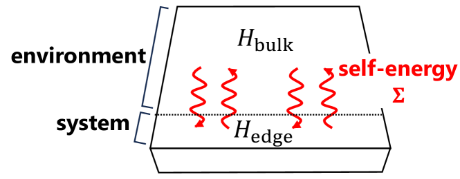
Figure 1: Effective non-Hermitian Hamiltonian $H_{\rm edge}+\Sigma$ at the edge of a Hermitian Hamiltonian. The self-energy $\Sigma$ describes the particle exchange between the bulk $H_{\rm bulk}$ and edge $H_{\rm edge}$, yielding non-Hermitian topology.

Non-Hermitian Hamiltonians in closed systems.—Our central idea involves conceptually dividing the bulk and boundary of a closed system into an environment and system, respectively (Fig. 1). The single-particle Hamiltonian of the entire system reads

$$H=\begin{pmatrix}H_{\rm bulk}&T\\ T^{{\dagger}}&H_{\rm edge}\end{pmatrix},$$ (1)

where $H_{\rm bulk}$ ($H_{\rm edge}$) is the Hamiltonian in the bulk (at the boundary), and $T$ denotes the coupling between the bulk and boundary. From the original Schrödinger equation $H\,(\ket{\psi}_{\rm bulk}\,\ket{\psi}_{\rm edge})^{T}=\left(E+\text{i}\eta\right)(\ket{\psi}_{\rm bulk}\,\ket{\psi}_{\rm edge})^{T}$ with an infinitesimal number $\eta>0$ reflecting causality, we project the boundary degree of freedom and derive the effective Hamiltonian $H_{\mathrm{eff}}\left(E\right)=H_{\mathrm{edge}}+\Sigma\left(E\right)$ with the self-energy [103, 104, 105]

$$\Sigma\left(E\right)\coloneqq T^{{\dagger}}\left(E+\text{i}\eta-H_{\rm bulk}\right)^{-1}T.$$ (2)

The self-energy $\Sigma\left(E\right)$ captures the continuous exchange of particles between the bulk and boundary for given energy $E\in\mathbb{R}$. Consequently, $\Sigma\left(E\right)$ acquires non-Hermiticity, describing finite lifetimes of quasiparticles that escape from the boundary to the bulk.

Crucially, topology of the original Hermitian Hamiltonian $H$ should leave an imprint on that of the effective non-Hermitian Hamiltonian $H_{\rm eff}\left(E\right)$. For example, when $H$ is a quantum Hall (Chern) insulator, $H_{\rm eff}\left(E\right)$ effectively describes chiral edge states for $E$ within an energy gap. Intuitively, chirality or nonreciprocity of the anomalous boundary states should yield non-Hermitian topology, as can be seen in the celebrated Hatano-Nelson model [106, *Hatano-Nelson-97]. In this Letter, we substantiate this intuition and demonstrate that the self-energy bridges Hermitian bulk topology and non-Hermitian boundary topology. Below, for fixed $E$ (i.e., Markov approximation [62, 108]), we study non-Hermitian topology of $H_{\rm eff}\left(E\right)$ in prototypical topological insulators.

Non-Hermitian topology in the Su-Schrieffer-Heeger model.—We begin with a one-dimensional topological insulator, Su-Schrieffer-Heeger (SSH) model [109]. The Bloch Hamiltonian reads

$$H_{\mathrm{SSH}}\left(k\right)=\left(v+t\cos{k}\right)\sigma_{x}+\left(t\sin{k}\right)\sigma_{y},$$ (3)

where $\sigma_{i}$’s ($i=x,y,z$) denote Pauli matrices, and $v>0$ and $t>0$ are the intracell and intercell hopping amplitudes, respectively.

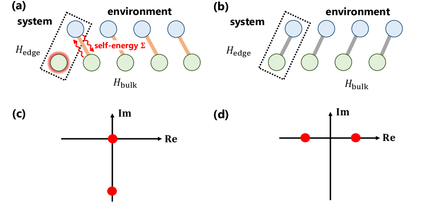
Figure 2: Non-Hermitian topology in the Su-Schrieffer-Heeger model. (a, b) Correspondence of Hermitian and non-Hermitian topology for the (a) nontrivial and (b) trivial phases. (c, d) Complex eigenvalues of the effective non-Hermitian Hamiltonian at the edge for the (c) nontrivial and (d) trivial phases.

The SSH model respects chiral symmetry $\sigma_{z}H_{\rm SSH}\left(k\right)\sigma_{z}=-H_{\rm SSH}\left(k\right)$ and belongs to class AIII, characterized by the integer topological invariant [7]. In the topological phase ($v/t<1$), the bulk topology leads to the emergence of an edge state $\ket{\psi_{0}}\propto\sum_{x}\left(-v/t\right)^{x}\ket{x}\otimes\left(1~{}0\right)^{T}$ with zero energy $E=0$ under the open boundary conditions. When we regard the unit cell at the left edge as a system and the remaining portion an environment [Fig. 2 (a, b)], the edge degree of freedom is coupled with the bulk and can escape into the bulk. This decaying property is quantified by the self-energy in Eq. (2), calculated as [105]

$$\Sigma\left(E\right)=\begin{pmatrix}0&0\\ 0&-\text{i}\pi\left(t^{2}-v^{2}\right)\delta\left(E\right)\theta\left(t-v\right)\end{pmatrix}.$$ (4)

The complex eigenvalues of the effective non-Hermitian Hamiltonian $H_{\rm eff}\left(0\right)=v\sigma_{x}+\Sigma\left(0\right)$ are obtained as $0$ and $-\text{i}\infty$, the former of which corresponds to a topologically stable zero state with an infinite lifetime and the latter of which an unstable zero state with a vanishing lifetime. In the trivial phase ($v/t>1$), by contrast, no eigenstates appear at $E=0$, and hence the self-energy vanishes $\Sigma\left(0\right)=0$.

Notably, the topological nature of the zero-energy edge state causes non-Hermitian topology of the effective Hamiltonian $H_{\rm eff}\left(0\right)$. In the topological phase, the two single-particle eigenenergies are gapped with a reference energy on the imaginary axis [Fig. 2 (c)], which is a non-Hermitian extension of energy gap called a point gap [20, 29]. Inheriting from chiral symmetry of the original SSH model $H_{\rm SSH}\left(k\right)$ in Eq. (3), the edge non-Hermitian Hamiltonian $H_{\rm eff}\left(0\right)$ also respects chiral symmetry $\sigma_{z}H_{\rm eff}^{{\dagger}}\left(0\right)\sigma_{z}=-H_{\rm eff}\left(0\right)$. Thanks to chiral symmetry, topologically-protected zero-energy states persist as long as the point gap is open. Such persistence is ensured by point-gap topology, given by the zeroth Chern number of the Hermitian matrix $\text{i}H_{\rm eff}\left(0\right)\sigma_{z}$ [29]. In fact, $H_{\rm eff}\left(0\right)=v\sigma_{x}+\Sigma\left(0\right)$ in Eq. (4) exhibits the zeroth Chern number $1$ ($0$) in the topological (trivial) phase. Thus, the self-energy $\Sigma\left(0\right)$ detects nontrivial Hermitian topology in the bulk and induces non-Hermitian topology at the edge.

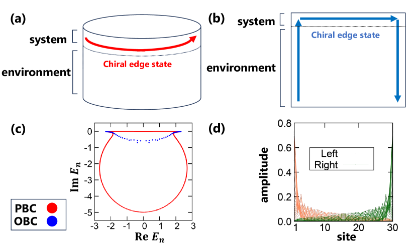
Figure 3: Non-Hermitian topology in the Chern insulator ($t=1.0$, $m=-1.3$, $E=0$). The open boundary conditions (OBC) are imposed along the $x$ direction. (a, b) Chiral edge state as a non-Hermitian subsystem of the Chern insulator. (c) Complex spectrum of the effective non-Hermitian Hamiltonian under the periodic boundary conditions (PBC; red; $L_{x}=3000$, $L_{y}=30$) and OBC (blue; $L_{x}=L_{y}=30$) along the $y$ direction. (d) Collection of all right (orange) and left (green) skin states. The infinitesimal number $\eta$ is chosen as $\eta=1/\sqrt{L_{y}}$ [110].

Non-Hermitian topology in a Chern insulator.—Next, we consider a Chern insulator on the square lattice described by [111, *QHZ-08]

$$H_{\mathrm{Chern}}\left(\bm{k}\right) =\left(t\sin{k_{x}}\right)\sigma_{x}+\left(t\sin{k_{y}}\right)\sigma_{y}$$

$$\qquad+\left(m+t\cos{k_{x}}+t\cos{k_{y}}\right)\sigma_{z}$$ (5)

with $t,m\in\mathbb{R}$. We regard the one-dimensional edge at $x=1$ as a system and the remaining bulk an environment, and show that the effective edge Hamiltonian yields non-Hermitian topology and concomitant skin effect (Fig. 3).

This model $H_{\mathrm{Chern}}\left(\bm{k}\right)$ is characterized by the first Chern number, obtained as $C_{1}=\mathrm{sgn}\left(m/t\right)$ ($C_{1}=0$) for $\left|m/t\right|<2$ ($\left|m/t\right|>2$). Imposing the open boundary conditions along the $x$ direction and periodic boundary conditions along the $y$ directions, we analytically obtain the self-energy [105]

$$\Sigma\left(E,k_{y}\right)=\frac{t^{2}-\left(m+t\cos{k_{y}}\right)^{2}}{2\left(E+\text{i}\eta-t\sin k_{y}\right)}\left(\sigma_{0}-\sigma_{y}\right).$$ (6)

We calculate the complex eigenvalues of the effective non-Hermitian Hamiltonian $H_{\rm eff}\left(E,k_{y}\right)=\left(t\sin k_{y}\right)\sigma_{y}+\left(m+t\cos k_{y}\right)\sigma_{z}+\Sigma\left(E,k_{y}\right)$ [Fig. 3 (c)]. These eigenvalues form a loop in the complex plane and host a point gap for reference energy $E_{0}$ inside the loop. This loop structure intuitively originates from chirality of the anomalous boundary states, in a similar manner to the Hatano-Nelson model [106, *Hatano-Nelson-97]. The nontrivial point-gap topology is captured by the winding of the complex spectrum,

$$W_{1}\coloneqq\oint\frac{dk}{2\pi\text{i}}\left(\frac{d}{dk}\log\det\left[H\left(k\right)-E_{0}\right]\right)$$ (7)

for a Bloch Hamiltonian $H\left(k\right)$ in one dimension [20, 29]. In fact, $H_{\rm eff}\left(E,k_{y}\right)$ with fixed $E$ exhibits $W_{1}=\mathrm{sgn}\left(m/t\right)$, leading to the correspondence $C_{1}=W_{1}$ between the Hermitian bulk and non-Hermitian boundary [99, 100].

The bulk-boundary correspondence for the nontrivial point-gap topology $W_{1}\neq 0$ manifests itself as the non-Hermitian skin effect [37, 38]. We calculate the complex spectrum of $H_{\rm eff}\left(E,k_{y}\right)$ under the open boundary conditions along both $x$ and $y$ directions [Fig. 3 (c)]. Clearly, the complex spectrum does not form a loop but an arc; such extreme sensitivity to the boundary conditions is a signature of the non-Hermitian skin effect [14, 22, 24]. Consistently, most of the right and left eigenstates of $H_{\rm eff}$ are localized at either corner of the square lattice [Fig. 3 (d)].

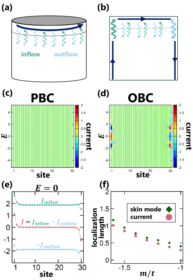
Figure 4: Localized current distribution due to the non-Hermitian skin effect. The open boundary conditions (OBC) are imposed along the $x$ direction. (a, b) While the inflow and outflow balance (a) under the periodic boundary conditions (PBC) along the $y$ direction, they do not (b) under OBC. (c, d) Terminal current for various energy $E$ under (c) PBC and (d) OBC ($t=1.0$, $m=-1.3$, $L_{x}=L_{y}=30$). (e) Inflow $J_{\rm inflow}$ (green), net current $J=J_{\rm inflow}-J_{\rm outflow}$ (red), and outflow $-J_{\rm outflow}$ (blue) for $E=0$. (f) Localization length of the current $J$ (red) and the most localized skin state (green) as functions of $m/t$, obtained from the scaling for the five sites near the boundary. The infinitesimal number $\eta$ is chosen as $\eta=1/\sqrt{L_{y}}$ [110].

Skin current.—We show that the non-Hermitian skin effect of the chiral edge states physically results in the localized current distribution (Fig. 4). Imposing the open boundary conditions along the $x$ direction, we investigate the $E$-resolved local current [105, 103, 113]

$$J\left(E\right)=-\big{[}H_{\mathrm{edge}},G_{\mathrm{edge}}\left(E\right)\big{]}-\big{[}H_{\mathrm{edge}},G_{\mathrm{edge}}\left(E\right)\big{]}^{\dagger},$$ (8)

with the edge Green’s function $G_{\rm edge}\left(E\right)\coloneqq\left(E+\text{i}\eta-H_{\mathrm{eff}}\left(E\right)\right)^{-1}$. Under the periodic boundary conditions along the $y$ direction, the inflow $J_{\rm inflow}$ and outflow $J_{\rm outflow}$ between the bulk and boundary balance, leading to the absence of the net current $J=J_{\rm inflow}-J_{\rm outflow}=0$. Under the open boundary conditions along the $y$ direction, by contrast, the nonzero net current $J$ arises around the corners. This unique current distribution results from the chiral edge states. In fact, chirality of the edge states leads to a large inflow at one corner and a large outflow at the opposite corner.

Notably, the localized current distribution is also a direct consequence of the corner skin effect. We find that the localization length of the current density shows behavior consistent with that of the skin states [Fig. 4 (f)]. A defining feature of the skin effect is the localization of right and left eigenstates at the opposite edges, as shown in Fig. 3 (d). From Eq. (8), a skin state with the localization length $\xi$ contributes to the the current density as $J_{y}\simeq j_{1}e^{-y/\xi}-j_{2}e^{-(L-y)/\xi}$ with constants $j_{1},j_{2}\in\mathbb{R}$, consistent with Fig. 4 (e, f). No local current arises if both right and left eigenstates of $H_{\rm eff}\left(E\right)$ are localized at the same boundary, as opposed to the skin states.

We also demonstrate the $\mathbb{Z}_{2}$ skin effect in a time-reversal-invariant topological insulator [114, 105]. It is also notable that similar $E$-dependent skin effect has been discussed in a recent work [115].

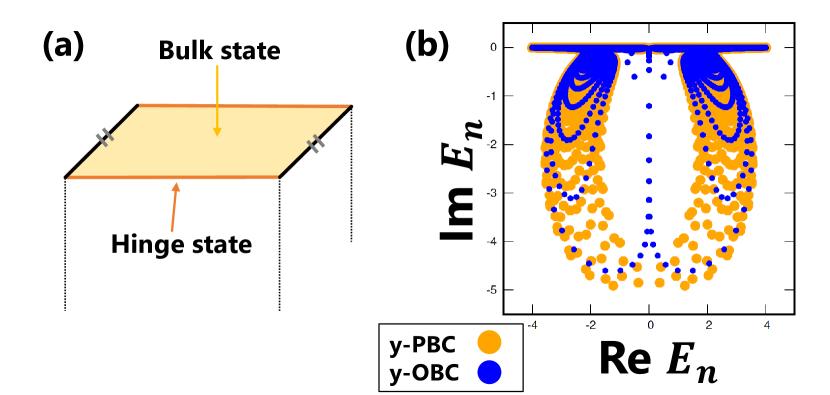
Figure 5: Non-Hermitian topology in a three-dimensional topological insulator. (a) Hinge state in an effective non-Hermitian Hamiltonian at a surface. (b) Complex spectrum of the effective non-Hermitian Hamiltonian under the periodic boundary conditions along the $y$ direction ($y$-PBC; orange; $L_{x}=L_{y}=200$, $L_{z}=30$) and open boundary conditions ($y$-OBC; blue; $L_{x}=200$, $L_{y}=L_{z}=30$) ($t=1.0$, $m=-1.6$, $\delta=0.2$). The periodic boundary conditions are imposed along the $x$ direction. The infinitesimal number $\eta$ is chosen as $\eta=1/\sqrt{L_{z}}$ [110].

Three dimensions.—We further study a three-dimensional topological insulator described by [4]

$$H_{\mathrm{3DTI}}\left(\bm{k}\right)=\left(m+t\cos{k_{x}}+t\cos{k_{y}}+t\cos{k_{z}}\right)\tau_{y}$$

$$\qquad+\left(t\sin{k_{x}}\right)\sigma_{x}\tau_{x}+\left(t\sin{k_{y}}\right)\sigma_{y}\tau_{x}$$

$$\qquad+\left(t\sin{k_{z}}\right)\sigma_{z}\tau_{x}+\delta\left(\cos{k_{x}}+\cos{k_{y}}\right)\sigma_{y}\tau_{y}$$ (9)

with Pauli matrices $\sigma_{i}$’s and $\tau_{i}$’s ($i=x,y,z$), and real parameters $m,t,\delta\in\mathbb{R}$. Similar to the SSH model, this Hamiltonian respects chiral symmetry $\tau_{z}H_{\mathrm{3DTI}}\left(\bm{k}\right)\tau_{z}=-H_{\mathrm{3DTI}}\left(\bm{k}\right)$ and is characterized by the three-dimensional winding number $W_{3}\in\mathbb{Z}$ [7]. In the topological phase, the nontrivial bulk topology $W_{3}\neq 0$ leads to the emergence of Dirac surface states. Applying the open boundary conditions along the $z$ direction, we regard the two-dimensional surface at $z=1$ as a system and the remaining bulk an environment (Fig. 5). The effective surface Hamiltonian $H_{\rm eff}\left(E,k_{x},k_{y}\right)$ hosts point-gap topology, characterized by the first Chern number of $\text{i}H_{\rm eff}\left(E,k_{x},k_{y}\right)\tau_{z}$. In contrast to the two-dimensional case, this point-gap topology does not result in the skin effect [38, 48]. Instead, anomalous hinge states with the imaginary dispersion $\propto\text{i}k_{x}$ appear. The distinct boundary physics should reflect the different nature of the coupling between the bulk and boundary.

Table 1: Periodic table of Hermitian topological insulators and superconductors in spatial dimensions $d=1,2,3$. The tenfold Altland-Zirnbauer (AZ) symmetry classes consist of time-reversal symmetry (TRS), particle-hole symmetry (PHS), and chiral symmetry (CS). In the entries specified by ^∗, effective non-Hermitian Hamiltonians at boundaries exhibit the skin effect; in 3D class DIII, specified by ^∗∗, the skin effect arises only for the odd number of the topological invariant [48].

AZ class	TRS	PHS	CS	$d=1$	$d=2$	$d=3$
A	$0$	$0$	$0$	$0$	$\mathbb{Z}^{*}$	$0$
AIII	$0$	$0$	$1$	$\mathbb{Z}$	$0$	$\mathbb{Z}$
AI	$+1$	$0$	$0$	0	0	0
BDI	$+1$	$+1$	$1$	$\mathbb{Z}$	0	0
D	$0$	$+1$	$0$	$\mathbb{Z}_{2}$	$\mathbb{Z}^{*}$	0
DIII	$-1$	$+1$	$1$	$\mathbb{Z}_{2}$	$\mathbb{Z}_{2}^{*}$	$\mathbb{Z}^{**}$
AII	$-1$	$0$	$0$	0	$\mathbb{Z}_{2}^{*}$	$\mathbb{Z}_{2}^{*}$
CII	$-1$	$-1$	$1$	$2\mathbb{Z}$	0	$\mathbb{Z}_{2}$
C	$0$	$-1$	$0$	0	$2\mathbb{Z}^{*}$	0
CI	$+1$	$-1$	$1$	0	0	$2\mathbb{Z}$

Classification.—While we have hitherto focused on the prototypical models, anomalous boundary states in topological insulators generally host non-Hermitian topology, as summarized in Table 1. In fact, when the original Hermitian Hamiltonians in Eq. (1) respect the Altland-Zirnbauer (AZ) symmetry [3, 7], the effective non-Hermitian Hamiltonians $H_{\rm eff}\left(E\right)=H_{\rm edge}+\Sigma\left(E\right)$ respect the corresponding symmetry known as the AZ^† symmetry [105, 29]. Consequently, $H_{\rm eff}\left(E\right)$ shows $d$-dimensional non-Hermitian topology inheriting from $\left(d+1\right)$-dimensional Hermitian topology. In Table 1, various boundary phenomena are classified based on symmetry and dimensions [38, 48]. For example, helical Dirac surface states of time-reversal-invariant topological insulators host the $\mathbb{Z}_{2}$ skin effect, contrasting with the chiral-symmetric topological insulator in Eq. (Non-Hermitian Topology in Hermitian Topological Matter).

Discussions.—In this Letter, we reveal intrinsic non-Hermitian topology of anomalous boundary states in Hermitian topological matter. We demonstrate that the self-energy quantifying the particle exchange between the bulk and boundary detects Hermitian topology in the bulk and non-Hermitian topology at the boundary. In Refs. [98, 99, 100], point-gap topology of anomalous boundary states was investigated in the presence of non-Hermitian external perturbations. In this Letter, by contrast, we show non-Hermitian topology inherently embedded within topological boundary states. Non-Hermitian topology was identified also in scattering matrices of Hermitian topological insulators [116, 117]. Conversely, we microscopically construct effective Hamiltonians and demonstrate their intrinsic non-Hermitian topology.

While we focus on clean noninteracting systems in this Letter, our formalism should be extended to topological matter with disorder or many-body interactions, which we investigate in future work. Additionally, it merits further study to develop a field-theoretical understanding of our correspondence. In this respect, our finding implies that anomaly of topological boundary states has a close connection with a different type of anomaly accompanying non-Hermitian topology [44]. It is also worthwhile to revisit fermion doubling from our perspective [118, 119, 120].

Supplemental Material for
“Non-Hermitian Topology in Hermitian Topological Matter”

I Effective non-Hermitian Hamiltonian

We consider an edge Hamiltonian $H_{\rm edge}$ that is attached to a bulk Hamiltonian $H_{\rm bulk}$. The whole system is described as

$$H=\begin{pmatrix}H_{\rm bulk}&T\\ T^{{\dagger}}&H_{\rm edge}\end{pmatrix},$$ (I.1)

where $T$ denotes the coupling between the bulk and the edge. The Green’s function $G$ of $H$ is defined by [103]

$$\left[\left(E+\text{i}\eta\right)-H\right]G=1,$$ (I.2)

or

$$\begin{pmatrix}E+\text{i}\eta-H_{\rm bulk}&-T\\ -T^{{\dagger}}&E+\text{i}\eta-H_{\rm edge}\end{pmatrix}\begin{pmatrix}G_{\rm bulk}&G_{\rm bulk-edge}\\ G_{\rm edge-bulk}&G_{\rm edge}\end{pmatrix}=1,$$ (I.3)

with an infinitesimal number $\eta>0$. This equation reads

$$\left(E+\text{i}\eta-H_{\rm bulk}\right)G_{\rm bulk-edge}-TG_{\rm edge} =0,$$ (I.4)

$$-T^{{\dagger}}G_{\rm bulk-edge}+\left(E+\text{i}\eta-H_{\rm edge}\right)G_{\rm edge} =1,$$ (I.5)

leading to

$$G_{\rm bulk-edge}=\left(E+\text{i}\eta-H_{\rm bulk}\right)^{-1}TG_{\rm edge}\eqqcolon G_{\rm bulk}^{(0)}TG_{\rm edge},$$ (I.6)

with the Green’s function $G_{\rm bulk}^{(0)}\coloneqq\left(E+\text{i}\eta-H_{\rm bulk}\right)^{-1}$ of the isolated bulk. Moreover, we have

$$\left(E+\text{i}\eta-H_{\rm edge}-\Sigma\right)G_{\rm edge}=1,$$ (I.7)

where we introduce the self-energy $\Sigma$ of the bulk as

$$\Sigma\coloneqq T^{{\dagger}}\left(E+\text{i}\eta-H_{\rm bulk}\right)^{-1}T=T^{{\dagger}}G_{\rm bulk}^{(0)}T.$$ (I.8)

The effective non-Hermitian Hamiltonian at the edge reads

$$H_{\rm eff}\coloneqq H_{\rm edge}+\Sigma=H_{\rm edge}+T^{{\dagger}}\left(E+\text{i}\eta-H_{\rm bulk}\right)^{-1}T.$$ (I.9)

Let $E_{n}$ be an eigenenergy of $H_{\rm bulk}$ and $\ket{\psi_{n}}$ be the corresponding eigenstate. Then, we have the spectral decomposition

$$\Sigma=T^{{\dagger}}\left(\sum_{n}\frac{\ket{\psi_{n}}\bra{\psi_{n}}}{E+\text{i}\eta-E_{n}}\right)T.$$ (I.10)

Example

As the simplest example, we consider a single-band model [122]

$$H_{ij}=t\left(\delta_{i,j+1}+\delta_{i,j-1}\right)\quad\left(t>0\right).$$ (I.11)

Let $\ket{\psi_{n}}=(\psi_{1}^{(n)},\psi_{2}^{(n)},\cdots,\psi_{L}^{(n)})$ be an eigenstate of $H_{\rm bulk}$. Then, the Schrödinger equation $H\ket{\psi_{n}}=E_{n}\ket{\psi_{n}}$ reads

$$t\psi_{j-1}^{(n)}+t\psi_{j+1}^{(n)}=E_{n}\psi_{j}^{(n)}\quad\left(j=2,3,\cdots,L-1\right),\quad\psi_{0}^{(n)}=\psi_{L+1}^{(n)}=0.$$ (I.12)

The eigenenergies and eigenstates are given as

$$E_{n}=2t\cos k_{n},\quad\psi_{j}^{(n)}=\sqrt{\frac{2}{L+1}}\sin\left(k_{n}j\right);\quad k_{n}\coloneqq\frac{n\pi}{L+1}\quad\left(n=1,2,\cdots,L\right).$$ (I.13)

Thus, the self-energy of the bulk is obtained as

$$\Sigma=t^{2}\sum_{n=1}^{L}\frac{|\psi_{j}^{(n)}|^{2}}{E+\text{i}\eta-E_{n}}=\frac{2t^{2}}{L+1}\sum_{n=1}^{L}\frac{\sin^{2}k_{n}}{E+\text{i}\eta-2t\cos k_{n}}.$$ (I.14)

In the semi-infinite limit $L\to\infty$, we have

$$\Sigma=2t^{2}\sum_{n=1}^{L}\frac{\Delta k_{n}}{\pi}\frac{\sin^{2}k_{n}}{E+\text{i}\eta-2t\cos k_{n}}\to 2t^{2}\int_{0}^{\pi}\frac{dk}{\pi}\frac{\sin^{2}k}{E+\text{i}\eta-2t\cos k}=\frac{E}{2}\left(1-\sqrt{1-\frac{4t^{2}}{E^{2}}}\right).$$ (I.15)

The imaginary part of $\Sigma$ appears for $E$ within the bulk bandwidth $\left|E\right|<2t$, which reflects the particle exchange between the bulk and the edge.

II Symmetry classification of non-Hermitian self-energy

We study symmetry of effective non-Hermitian Hamiltonians introduced in Sec. I. Specifically, we show that when original Hermitian Hamiltonians belong to the Altland-Zirnbauer symmetry class [3], the corresponding effective non-Hermitian Hamiltonians belong to the Altland-Zirnbauer^† symmetry class [29]. The similar correspondence was derived, for example, for quadratic Lindbladians [123] and reflection matrices in scattering processes [124]. Because of this correspondence, the topological classification of $d$-dimensional Hermitian Hamiltonians coincides with that of $\left(d-1\right)$-dimensional effective non-Hermitian Hamiltonians [29, 92, 93, 99, 100].

II.1 Time-reversal symmetry

Suppose that the original Hermitian Hamiltonian $H$ respects time-reversal symmetry:

$$\mathcal{T}H^{*}\mathcal{T}^{-1}=H$$ (II.1)

with a unitary matrix $\mathcal{T}$. Since time reversal acts only on the internal degrees of freedom, we have

$$\mathcal{T}H^{*}_{\rm bulk}\mathcal{T}^{-1}=H_{\rm bulk},\quad\mathcal{T}H^{*}_{\rm edge}\mathcal{T}^{-1}=H_{\rm edge},\quad\mathcal{T}T^{*}\mathcal{T}^{-1}=T.$$ (II.2)

Consequently, we have

$$\mathcal{T}\Sigma^{T}\left(E\right)\mathcal{T}^{-1}=T^{{\dagger}}\left(E+\text{i}\eta-H_{\rm bulk}\right)^{-1}T=\Sigma\left(E\right),$$ (II.3)

and hence

$$\mathcal{T}H_{\rm eff}^{T}\left(E\right)\mathcal{T}^{-1}=H_{\rm eff}\left(E\right).$$ (II.4)

Thus, for arbitrary $E$, the effective non-Hermitian Hamiltonian $H_{\rm eff}$ respects time-reversal symmetry^† [29]. Notably, $H_{\rm eff}$ is not invariant under time reversal (i.e., $\mathcal{T}H_{\rm eff}^{*}\mathcal{T}^{-1}\neq H_{\rm eff}$).

II.2 Particle-hole symmetry

Suppose that the original Hermitian Hamiltonian $H$ respects particle-hole symmetry:

$$\mathcal{C}H^{*}\mathcal{C}^{-1}=-H$$ (II.5)

with a unitary matrix $\mathcal{C}$. Since particle-hole transformation acts only on the internal degrees of freedom, we have

$$\mathcal{C}H^{*}_{\rm bulk}\mathcal{C}^{-1}=-H_{\rm bulk},\quad\mathcal{C}H^{*}_{\rm edge}\mathcal{C}^{-1}=-H_{\rm edge},\quad\mathcal{C}T^{*}\mathcal{C}^{-1}=-T.$$ (II.6)

Consequently, we have

$$\mathcal{C}\Sigma^{*}\left(E\right)\mathcal{C}^{-1}=T^{{\dagger}}\left(E-\text{i}\eta+H_{\rm bulk}\right)^{-1}T=-\Sigma\left(-E\right),$$ (II.7)

and hence

$$\mathcal{C}H_{\rm eff}^{*}\left(E\right)\mathcal{C}^{-1}=-H_{\rm eff}\left(-E\right).$$ (II.8)

Thus, at the particle-hole-symmetric point $E=0$, the effective non-Hermitian Hamiltonian $H_{\rm eff}\left(E=0\right)$ respects particle-hole symmetry^† [29]. Notably, $H_{\rm eff}$ does not respect particle-hole symmetry even at $E=0$ [i.e., $\mathcal{C}H_{\rm eff}^{T}\left(E=0\right)\mathcal{C}^{-1}\neq-H_{\rm eff}\left(E=0\right)$].

II.3 Chiral symmetry

Suppose that the original Hermitian Hamiltonian $H$ respects chiral symmetry:

$$\Gamma H\Gamma^{-1}=-H$$ (II.9)

with a unitary matrix $\Gamma$. Since chiral transformation acts only on the internal degrees of freedom, we have

$$\Gamma H_{\rm bulk}\Gamma^{-1}=-H_{\rm bulk},\quad\Gamma H_{\rm edge}\Gamma^{-1}=-H_{\rm edge},\quad\Gamma T\Gamma^{-1}=-T.$$ (II.10)

Consequently, we have

$$\Gamma\Sigma^{{\dagger}}\left(E\right)\Gamma^{-1}=T^{{\dagger}}\left(E-\text{i}\eta+H_{\rm bulk}\right)^{-1}T=-\Sigma\left(-E\right),$$ (II.11)

and hence

$$\Gamma H_{\rm eff}^{{\dagger}}\left(E\right)\Gamma^{-1}=-H_{\rm eff}\left(-E\right).$$ (II.12)

Thus, at the chiral-symmetric point $E=0$, the effective non-Hermitian Hamiltonian $H_{\rm eff}\left(E=0\right)$ respects chiral symmetry [29]. Notably, $H_{\rm eff}$ does not respect sublattice symmetry even at $E=0$ [i.e., $\Gamma H_{\rm eff}\left(E=0\right)\Gamma^{-1}\neq-H_{\rm eff}\left(E=0\right)$].

III Analytical derivation of the self-energy

We analytically derive the self-energy between the bulk and boundaries for the Su-Schrieffer-Heeger (SSH) model and a Chern insulator.

III.1 Su-Schrieffer-Heeger model

We consider the SSH model [109]

$$H_{\mathrm{bulk}}\left(k\right)=\left(v+t\cos{k}\right)\sigma_{x}+\left(t\sin{k}\right)\sigma_{y},$$ (III.1)

where $\sigma_{i}$’s ($i=x,y,z$) are Pauli matrices, and $v>0$ and $t>0$ are the intracell and intercell hopping amplitudes, respectively. Below, we assume the open boundary conditions. In the topologically nontrivial phase $r<1$ ($r\coloneqq v/t$), a pair of zero-energy states appears at the boundaries. We assume that the total number of sites is odd, $2L+1$, for the sake of simplicity, for which eigenstates are exactly obtained under the open boundary conditions (see, for example, Refs. [121, 125]). Let $\ket{\psi_{n}}=(\psi_{1}^{(n)},\psi_{2}^{(n)},\cdots,\psi_{2L+1}^{(n)})$ be an eigenstate. The bulk states host the eigenenergy

$$E_{n}=\pm t\sqrt{r^{2}+1+2r\cos{k_{n}}}\quad\left(k_{n}\coloneqq\frac{n\pi}{L+1};~{}n=1,\cdots,L\right),$$ (III.2)

and the corresponding bulk eigenstates are obtained as

$$\psi_{2j-1}^{(n)}=\frac{r\sin\left(k_{n}j\right)+\sin\left(k_{n}(j-1)\right)}{\sqrt{(L+1)\left(1+2r\cos{k_{n}}+r^{2}\right)}}\hskip 14.22636pt\left(j=1,\cdots,L+1\right),\quad\quad~{}\psi_{2j}^{(n)}=\pm\frac{\sin{\left(k_{n}j\right)}}{L+1}\hskip 14.22636pt\left(j=1,\cdots,L\right).$$ (III.3)

On the other hand, the zero-energy eigenstate localized at the left edge is given as

$$\psi_{2j}=0\hskip 14.22636pt\left(j=1,\cdots,L\right),\quad\quad\psi_{2j+1} =(-r)^{j}\sqrt{\frac{1-r^{2}}{1-r^{2(L+1)}}}\hskip 14.22636pt\left(j=0,\cdots,L\right)$$ (III.4)

for $r<1$.

Now, we compute the self-energy $\Sigma=\Sigma_{\mathrm{edge}}+\Sigma_{\mathrm{bulk}}$. The contribution $\Sigma_{\mathrm{edge}}$ from the edge state is obtained as

$$\Sigma_{\mathrm{edge}}=\frac{t^{2}(1-r^{2})}{1-{r}^{2(L+1)}}\frac{1}{E+\text{i}\eta}\frac{\sigma_{0}-\sigma_{z}}{2}\rightarrow\frac{t^{2}(1-r^{2})}{E+\text{i}\eta}\frac{\sigma_{0}-\sigma_{z}}{2}$$ (III.5)

in the limit $L\rightarrow\infty$ for $r<1$. Here, $\sigma_{0}$ is the $2\times 2$ identity matrix. Next, from Eqs. (III.2) and (III.3), the self-energy $\Sigma_{\mathrm{bulk}}$ from the bulk states is obtained as

$$\Sigma_{\mathrm{bulk}}= \frac{t^{2}}{L+1}\sum\limits_{n=1}^{L}\frac{r^{2}\sin^{2}{k_{n}}}{r^{2}+1+2r\cos{k_{n}}}\Biggl{(}\frac{1}{E+\text{i}\eta-t\sqrt{r^{2}+1+2r\cos{k_{n}}}}+\frac{1}{E+\text{i}\eta+t\sqrt{r^{2}+1+2r\cos{k_{n}}}}\Biggr{)}\frac{\sigma_{0}-\sigma_{z}}{2}$$

$$\rightarrow\, t^{2}\int_{0}^{\pi}\frac{dk}{\pi}\frac{r^{2}\sin^{2}{k}}{r^{2}+1+2r\cos{k}}\Biggl{(}\frac{1}{E+\text{i}\eta-t\sqrt{r^{2}+1+2r\cos{k}}}+\frac{1}{E+\text{i}\eta+t\sqrt{r^{2}+1+2r\cos{k}}}\Biggr{)}\frac{\sigma_{0}-\sigma_{z}}{2}$$ (III.6)

for $L\rightarrow\infty$. By introducing the complex variable $z=e^{\text{i}k}$, the self-energy further leads to the contour integral

$$\Sigma_{\mathrm{bulk}}\rightarrow\frac{E+\text{i}\eta}{2}\frac{\sigma_{0}-\sigma_{z}}{2}\frac{1}{2\pi\text{i}}\oint_{C}dz~{}f(z),$$ (III.7)

where $C$ is the unit circle in the complex plane, and $f(z)$ is defined as

$$f(z)\coloneqq\frac{1}{z}\frac{(z^{2}-1)^{2}}{z^{2}+\left(r+r^{-1}\right)z+1}\frac{1}{z^{2}+2uz+1},\quad 2u\coloneqq\left(r+\frac{1}{r}\right)-\frac{1}{r}\left(\frac{E+\text{i}\eta}{t}\right)^{2}.$$ (III.8)

The poles of $f(z)$ are

$$z=0,-r,-\frac{1}{r},z_{\pm},\quad\left(z_{\pm}\coloneqq-u\pm\sqrt{u^{2}-1}\right),$$ (III.9)

whose residues are calculated as

$$\Res[z=0]=1,~{}\Res[z=-r]=-\frac{t^{2}(1-r^{2})}{\left({E+\text{i}\eta}\right)^{2}},~{}\Res[z=-\frac{1}{r}]=\frac{t^{2}(1-r^{2})}{\left({E+\text{i}\eta}\right)^{2}},~{}\Res[z=z_{\pm}]=\pm\frac{2t^{2}r\sqrt{u^{2}-1}}{\left({E+\text{i}\eta}\right)^{2}}.$$ (III.10)

Depending on $r$, each pole is either located inside or outside the unit circle $C$, as summarized in the following:

1. For $r>1$ and $E^{2}<t^{2}(r^{2}+1)$, only the three poles $z=0,-r^{-1},z_{+}$ are located inside the unit circle $C$, leading to

   $$\Sigma_{\mathrm{bulk}}=\left(\frac{E+\text{i}\eta}{2}+\frac{1}{2}\frac{t^{2}(1-r^{2})}{E+\text{i}\eta}+\frac{1}{2}\frac{\sqrt{\left[t^{2}(r^{2}+1)-\left(E+\text{i}\eta\right)^{2}\right]^{2}-4t^{4}r^{2}}}{E+\text{i}\eta}\right)\frac{\sigma_{0}-\sigma_{z}}{2}.$$ (III.11)

2. For $r>1$ and $E^{2}>t^{2}(r^{2}+1)$, only the three poles $z=0,-r^{-1},z_{-}$ are located inside the unit circle $C$, leading to

   $$\Sigma_{\mathrm{bulk}}=\left(\frac{E+\text{i}\eta}{2}+\frac{1}{2}\frac{t^{2}(1-r^{2})}{E+\text{i}\eta}-\frac{1}{2}\frac{\sqrt{\left[t^{2}(r^{2}+1)-\left(E+\text{i}\eta\right)^{2}\right]^{2}-4t^{4}r^{2}}}{E+\text{i}\eta}\right)\frac{\sigma_{0}-\sigma_{z}}{2}.$$ (III.12)

3. For $r<1$ and $E^{2}<t^{2}(r^{2}+1)$, only the three poles $z=0,-r,z_{+}$ are located inside the unit circle $C$, leading to

   $$\Sigma_{\mathrm{bulk}}=\left(\frac{E+\text{i}\eta}{2}-\frac{1}{2}\frac{t^{2}(1-r^{2})}{E+\text{i}\eta}+\frac{1}{2}\frac{\sqrt{\left[t^{2}(r^{2}+1)-\left(E+\text{i}\eta\right)^{2}\right]^{2}-4t^{4}r^{2}}}{E+\text{i}\eta}\right)\frac{\sigma_{0}-\sigma_{z}}{2}.$$ (III.13)

4. For $r<1$ and $E^{2}>t^{2}(r^{2}+1)$, only the three poles $z=0,-r,z_{-}$ are located inside the unit circle $C$, leading to

   $$\Sigma_{\mathrm{bulk}}=\left(\frac{E+\text{i}\eta}{2}-\frac{1}{2}\frac{t^{2}(1-r^{2})}{E+\text{i}\eta}-\frac{1}{2}\frac{\sqrt{\left[t^{2}(r^{2}+1)-\left(E+\text{i}\eta\right)^{2}\right]^{2}-4t^{4}r^{2}}}{E+\text{i}\eta}\right)\frac{\sigma_{0}-\sigma_{z}}{2}.$$ (III.14)

Combining both contributions from the bulk and edge, we obtain the total self-energy as

$$\Sigma(E)=\left(\frac{E+\text{i}\eta}{2}+\frac{1}{2}\frac{t^{2}(1-r^{2})}{E+\text{i}\eta}+\frac{1}{2}\mathrm{sgn}\left[t^{2}(r^{2}+1)-E^{2}\right]\frac{\sqrt{\left[t^{2}(r^{2}+1)-\left(E+\text{i}\eta\right)^{2}\right]^{2}-4t^{4}r^{2}}}{E+\text{i}\eta}\right)\frac{\sigma_{0}-\sigma_{z}}{2}.$$ (III.15)

The imaginary part of the self-energy appears for $E$ within the bulk bandwidth $\left|v-t\right|<\left|E\right|<\left|v+t\right|$ or for zero energy $E=0$. At the critical point $r=1$, Eq. (III.15) reduces to Eq. (I.15). Additionally, at zero energy $E=0$, the self-energy reduces to

$$\Sigma(0)=\begin{cases}0\hskip 14.22636pt&(r>1);\\ -\text{i}\pi t^{2}(1-r^{2})\delta(0)\left(\sigma_{0}-\sigma_{z}\right)/2\hskip 14.22636pt&(r<1).\end{cases}$$ (III.16)

Thus, in the topologically nontrivial phase ($r<1$), the imaginary part of the self-energy diverges.

III.2 Chern insulator

We consider the Chern insulator [111]

$$H_{\mathrm{bulk}}\left(k_{x},k_{y}\right)=\left(t\sin{k_{x}}\right)\sigma_{x}+\left(t\sin{k_{y}}\right)\sigma_{y}+\left(m+t\cos{k_{x}}+t\cos{k_{y}}\right)\sigma_{z}$$ (III.17)

with Pauli matrices $\sigma_{i}$’s ($i=x,y,z$). Here, $t>0$, denotes the hopping amplitude, and $m\in\mathbb{R}$ denotes the onsite potential. We assume the square lattice under the open boundary conditions along the $x$ direction and the periodic boundary conditions along the $y$ direction. Defining $R(k_{y})$ and $S$ as

$$R(k_{y})\coloneqq\left(t\sin{k_{y}}\right)\sigma_{y}+\left(m+t\cos{k_{y}}\right)\sigma_{z},\quad S\coloneqq\frac{t}{2}\left(\sigma_{z}-\text{i}\sigma_{x}\right),$$ (III.18)

we express the Hamiltonian as

$$H_{\mathrm{bulk}}(k_{y})=\sum\limits_{x=1}^{L}\ket{x}\bra{x}\otimes R(k_{y})+\sum\limits_{x=1}^{L-1}\Bigg{[}\ket{x}\bra{x+1}\otimes S+\ket{x+1}\bra{x}\otimes S^{\dagger}\Bigg{]}.$$ (III.19)

In the topologically nontrivial phase $\absolutevalue{m}<2t$, a chiral edge state appears around the boundaries $x=1$ and $x=L$. We use the ansatz

$$\ket{\psi_{\mathrm{edge}}\left(k_{y}\right)}=\sum\limits_{x=1}^{L}\beta^{x}\left(k_{y}\right)\ket{x}\otimes\ket{u\left(k_{y}\right)}$$ (III.20)

for the chiral edge state localized around $x=1$ with a $k_{y}$-dependent two-component vector $\ket{u\left(k_{y}\right)}$. Here, $-1/\log\left|\beta\left(k_{y}\right)\right|$ gives a $k_{y}$-dependent localization length of the chiral edge state along the $x$ direction. Then, we reduce the eigenvalue equation $H_{\mathrm{bulk}}(k_{y})\ket{\psi_{\mathrm{edge}}(k_{y})}=\lambda_{\mathrm{edge}}(k_{y})\ket{\psi_{\mathrm{edge}}(k_{y})}$ to

$$\left(R\left(k_{y}\right)+S\beta\left(k_{y}\right)+S^{{\dagger}}\beta^{-1}\left(k_{y}\right)\right)\ket{u\left(k_{y}\right)} =\lambda_{\mathrm{edge}}(k_{y})\ket{u\left(k_{y}\right)}\hskip 28.45274pt(2\leq x\leq L-1)$$ (III.21)

in the bulk and

$$\left(R\left(k_{y}\right)+S\beta\left(k_{y}\right)\right)\ket{u\left(k_{y}\right)} =\lambda_{\mathrm{edge}}(k_{y})\ket{u\left(k_{y}\right)}\hskip 28.45274pt(x=1)$$ (III.22)

at the left edge. From these equations, we have

$$S^{\dagger}\ket{u\left(k_{y}\right)}=0,$$ (III.23)

further leading to

$$\ket{u\left(k_{y}\right)}=\left(\begin{array}[]{c}1\\ \text{i}\end{array}\right).$$ (III.26)

Combining Eqs. (III.22) and (III.26), we obtain

$$\left[-\frac{\text{i}t}{2}\beta\left(k_{y}\right)\sigma_{x}+\left(t\sin k_{y}\right)\sigma_{y}+\left(m+\cos k_{y}+\frac{t}{2}\beta\left(k_{y}\right)\right)\sigma_{z}\right]\ket{u}=\lambda_{\mathrm{edge}}(k_{y})\ket{u}.$$ (III.27)

From Eq. (III.27), $\lambda_{\mathrm{edge}}\left(k_{y}\right)$ and $\beta\left(k_{y}\right)$ are given as

$$\lambda_{\mathrm{edge}}(k_{y})=t\sin{k_{y}},\quad\beta(k_{y})=-\left(\frac{m}{t}+\cos k_{y}\right).$$ (III.28)

Thus, the self-energy is calculated as

$$\Sigma_{\mathrm{edge}}(k_{y})=\frac{t^{2}(1-\beta^{2})}{2(E+\text{i}\eta-t\sin k_{y})}(\sigma_{0}-\sigma_{y}).$$ (III.29)

For $k_{y}=0$ or $k_{y}=\pi$, this self-energy essentially reduces to that of the SSH model [see Eq. (III.5)]. Notably, these expressions are valid only for

$$1>\absolutevalue{\beta}=\absolutevalue{\frac{m}{t}+\cos{k_{y}}}$$ (III.30)

so that the above chiral edge state can be normalized.

IV Current formula

We derive the current formula in Eq. (8) of the main text (see also “Chapter 8: Non-equilibrium Green’s function formalism” in Ref. [103], as well as “Chapter 9: Coherent transport” and “Appendix: advanced formalism” in Ref. [113]). We consider a noninteracting fermionic Hamiltonian described by

$$\hat{H}=\sum_{i,j}\hat{a}_{i}^{\dagger}H_{ij}\hat{a}_{j},$$ (IV.1)

where $\hat{a}_{i}$ ($\hat{a}^{\dagger}_{i}$) is a fermionic annihilation (creation) operator at site $i$, and $H_{ij}$ is a single-particle Hermitian Hamiltonian. The Heisenberg equation for the annihilation operator reads

$$\text{i}\hbar\frac{d\hat{a}_{i}(t)}{dt}=[\hat{a}_{i}(t),\hat{H}]=\sum_{j}H_{ij}\hat{a}_{j}(t).$$ (IV.2)

We rewrite this equation as

$$\text{i}\hbar\frac{d}{dt}\begin{pmatrix}\hat{\boldsymbol{a}}_{\mathrm{bulk}}(t)\\ \hat{\boldsymbol{a}}_{\mathrm{edge}}(t)\end{pmatrix}=\begin{pmatrix}H_{\rm bulk}&T\\ T^{{\dagger}}&H_{\rm edge}\end{pmatrix}\begin{pmatrix}\hat{\boldsymbol{a}}_{\mathrm{bulk}}(t)\\ \hat{\boldsymbol{a}}_{\mathrm{edge}}(t)\end{pmatrix},$$ (IV.3)

where $\hat{\boldsymbol{a}}_{\mathrm{bulk}}(t)$ [$\hat{\boldsymbol{a}}_{\mathrm{edge}}(t)$] is a row vector of annihilation operators acting on the bulk (edge). We expand the annihilation operator for the bulk as

$$\hat{\boldsymbol{a}}_{\mathrm{bulk}}(t)=\hat{\boldsymbol{a}}_{\mathrm{bulk}}^{(0)}(t)+\hat{\boldsymbol{\chi}}(t),$$ (IV.4)

where $\hat{\boldsymbol{a}}_{\mathrm{bulk}}^{(0)}(t)$ denotes the unperturbed annihilation operator satisfying $\text{i}\hbar\left(d/dt\right)\hat{\boldsymbol{a}}_{\mathrm{bulk}}^{(0)}(t)=H_{\rm bulk}\hat{\boldsymbol{a}}_{\mathrm{bulk}}^{(0)}(t)$. From the original Heisenberg equation in Eq. (IV.3), we have

$$\left(\text{i}\hbar\frac{d}{dt}-H_{\rm bulk}\right)\hat{\boldsymbol{\chi}}(t) =T\hat{\boldsymbol{a}}_{\mathrm{edge}}(t),$$ (IV.5)

$$\left(\text{i}\hbar\frac{d}{dt}-H_{\rm edge}\right)\hat{\boldsymbol{a}}_{\mathrm{edge}}(t) =T^{\dagger}\left(\hat{\boldsymbol{a}}_{\mathrm{bulk}}^{(0)}(t)+\hat{\boldsymbol{\chi}}(t)\right).$$ (IV.6)

We introduce the retarded Green’s function $g^{(0)}_{\mathrm{bulk}}(t-t^{\prime})$ for the bulk

$$\left(\text{i}\hbar\frac{d}{dt}-H_{\rm bulk}\right)g^{(0)}_{\mathrm{bulk}}(t-t^{\prime})=\delta(t-t^{\prime}).$$ (IV.7)

Here, the argument of the Green’s function depends only on the time difference $t-t^{\prime}$ since the Hamiltonian $H_{\mathrm{bulk}}$ is independent of time. Using the Green’s function, we obtain the formal solution of Eq. (IV.5) by the convolution integral,

$$\hat{\boldsymbol{\chi}}(t)=\int dt^{\prime}g^{(0)}_{\mathrm{bulk}}(t-t^{\prime})T\hat{\boldsymbol{a}}_{\mathrm{edge}}(t^{\prime}),$$ (IV.8)

and hence

$$\left(\text{i}\hbar\frac{d}{dt}-H_{\rm edge}\right)\hat{\boldsymbol{a}}_{\mathrm{edge}}(t)=T^{\dagger}\hat{\boldsymbol{a}}_{\mathrm{bulk}}^{(0)}(t)+\int dt^{\prime}\Sigma(t-t^{\prime})\hat{\boldsymbol{a}}_{\mathrm{edge}}(t^{\prime})$$ (IV.9)

with the self-energy defined as

$$\Sigma(t-t^{\prime})\coloneqq T^{\dagger}g^{(0)}_{\mathrm{bulk}}(t-t^{\prime})T.$$ (IV.10)

Similarly, introducing the retarded Green’s function $g_{\mathrm{edge}}(t-t^{\prime})$ for the edge by

$$\left(\text{i}\hbar\frac{d}{dt}-H_{\rm edge}\right)g_{\mathrm{edge}}(t-t^{\prime})=\int dt^{\prime\prime}\Sigma(t-t^{\prime\prime})g_{\mathrm{edge}}(t^{\prime\prime}-t^{\prime})+\delta(t-t^{\prime}),$$ (IV.11)

we obtain the formal solution of Eq. (IV.9) as

$$\hat{\boldsymbol{a}}_{\mathrm{edge}}(t)=\int dt^{\prime}g_{\mathrm{edge}}(t-t^{\prime})T^{\dagger}\hat{\boldsymbol{a}}_{\mathrm{bulk}}^{(0)}(t^{\prime}).$$ (IV.12)

Similar calculations for the creation operator lead to

$$\left(\text{i}\hbar\frac{d}{dt}+H_{\rm edge}^{T}\right)\hat{\boldsymbol{a}}_{\mathrm{edge}}^{\dagger}(t)=-\int dt^{\prime}\Sigma^{*}(t-t^{\prime})\hat{\boldsymbol{a}}_{\mathrm{edge}}^{\dagger}(t^{\prime})-T^{T}\hat{\boldsymbol{a}}_{\mathrm{bulk}}^{(0)^{{\dagger}}}(t)$$ (IV.13)

and hence

$$\hat{\boldsymbol{a}}_{\mathrm{edge}}^{\dagger}(t)=\int dt^{\prime}g_{\mathrm{edge}}^{*}(t-t^{\prime})T^{T}\hat{\boldsymbol{a}}_{\mathrm{bulk}}^{(0)^{{\dagger}}}(t^{\prime}).$$ (IV.14)

We define the Fourier transform of $f(t-t^{\prime})$ as

$$\mathcal{F}\left[f(t-t^{\prime})\right]\coloneqq\int d(t-t^{\prime})e^{\text{i}\frac{E}{\hbar}(t-t^{\prime})}f(t-t^{\prime}).$$ (IV.15)

The Fourier transforms of the Green’s functions $g^{(0)}_{\mathrm{bulk}}(t-t^{\prime})$ in Eq. (IV.7) and $g_{\mathrm{edge}}(t-t^{\prime})$ in Eq. (IV.11) are

$$G_{\mathrm{bulk}}^{(0)}(E)\coloneqq\mathcal{F}\left[g_{\mathrm{bulk}}^{(0)}(t-t^{\prime})\right]=\frac{1}{E+\text{i}\eta-H_{\mathrm{bulk}}},\quad G_{\mathrm{edge}}(E)\coloneqq\mathcal{F}\left[g_{\mathrm{edge}}(t-t^{\prime})\right]=\frac{1}{E+\text{i}\eta-H_{\mathrm{edge}}-\Sigma(E)},$$ (IV.16)

with $\Sigma(E)\coloneqq\mathcal{F}\left[\Sigma(t-t^{\prime})\right]$. Here, an infinitesimal number $\eta>0$ is introduced so that the initial condition can be satisfied appropriately.

Now, we introduce the two-time current operator [103, 113]

$$J(t,t^{\prime})\coloneqq\left(\frac{d}{dt}+\frac{d}{dt^{\prime}}\right)C(t,t^{\prime}),$$ (IV.17)

with the two-time correlation function

$$C_{ij}(t,t^{\prime})\coloneqq\langle\hat{a}_{j}^{\dagger}(t^{\prime})\hat{a}_{i}(t)\rangle,$$ (IV.18)

where the bracket denotes the average over a thermal equilibrium state. In the limit $t^{\prime}\rightarrow t$, the diagonal element of $J(t,t^{\prime})$ gives the local current. From Eqs. (IV.12) and (IV.13), the correlation function of the edge, $C_{\mathrm{edge};ij}(t,t^{\prime})\coloneqq\langle\hat{a}_{{\mathrm{edge}};j}^{\dagger}(t^{\prime})\hat{a}_{{\mathrm{edge}};i}(t)\rangle$, satisfies

$$\text{i}\hbar\frac{d}{dt}C_{\mathrm{edge}}(t,t^{\prime})=-C_{\mathrm{edge}}(t,t^{\prime})H_{\mathrm{edge}}-\int dt^{\prime\prime}g_{\mathrm{edge}}(t^{\prime},t^{\prime\prime})T^{\dagger}C_{\mathrm{bulk}}^{(0)}(t,t^{\prime\prime})T-\int dt^{\prime\prime}C_{\mathrm{edge}}(t^{\prime\prime},t^{\prime})\Sigma^{\dagger}(t,t^{\prime\prime}),$$ (IV.19)

with the isolated bulk correlation function $C_{\mathrm{bulk};ij}^{(0)}(t,t^{\prime})\coloneqq\langle\hat{a}^{(0)^{{\dagger}}}_{\mathrm{bulk};j}(t^{\prime})\hat{a}^{(0)}_{\mathrm{bulk};i}(t)\rangle$. Here, we assume that the bulk maintains the local equilibrium even after attaching the edge [103, 113]. Similarly, from Eqs. (IV.9) and (IV.14), we have

$$\text{i}\hbar\frac{d}{dt^{\prime}}C_{\mathrm{edge}}(t,t^{\prime})=H_{\mathrm{edge}}C_{\mathrm{edge}}(t,t^{\prime})+\int dt^{\prime\prime}T^{\dagger}C_{\mathrm{bulk}}^{(0)}(t^{\prime\prime},t^{\prime})Tg_{\mathrm{edge}}^{\dagger}(t,t^{\prime\prime})+\int dt^{\prime\prime}\Sigma(t^{\prime},t^{\prime\prime})C_{\mathrm{edge}}(t,t^{\prime\prime}).$$ (IV.20)

The first term of the right-hand side in Eqs. (IV.19) and (IV.20) represents the particle current inside the edge; we below omit it since it is irrelevant to the current between the bulk and edge, and hence non-Hermitian topology. Additionally, the second (third) term in Eqs. (IV.19) and (IV.20) describes the particle current from the bulk to the edge (from the edge to the bulk). Then, the net current is

$$J(t,t^{\prime})=J_{\mathrm{inflow}}(t,t^{\prime})-J_{\mathrm{outflow}}(t,t^{\prime})$$ (IV.21)

with

$$\text{i}\hbar J_{\mathrm{inflow}}(t,t^{\prime}) \coloneqq-\int dt^{\prime\prime}g_{\mathrm{edge}}(t^{\prime},t^{\prime\prime})T^{\dagger}C_{\mathrm{bulk}}^{(0)}(t,t^{\prime\prime})T+\int dt^{\prime\prime}T^{\dagger}C_{\mathrm{bulk}}^{(0)}(t^{\prime\prime},t^{\prime})Tg_{\mathrm{edge}}^{\dagger}(t,t^{\prime\prime}),$$ (IV.22)

$$\text{i}\hbar J_{\mathrm{outflow}}(t,t^{\prime}) \coloneqq\int dt^{\prime\prime}C_{\mathrm{edge}}(t^{\prime\prime},t^{\prime})\Sigma^{\dagger}(t,t^{\prime\prime})-\int dt^{\prime\prime}\Sigma(t^{\prime},t^{\prime\prime})C_{\mathrm{edge}}(t,t^{\prime\prime}).$$ (IV.23)

At thermal equilibrium, from the cyclicity of the trace, the correlation functions $C_{\mathrm{bulk}}^{(0)}(t,t^{\prime})$ and $C_{\mathrm{edge}}(t,t^{\prime})$ depend only on the argument $t-t^{\prime}$. After the Fourier transformation, the $E$-resolved currents read,

$$\text{i}\hbar J_{\mathrm{inflow}}(E) \coloneqq\mathcal{F}\left[J_{\mathrm{inflow}}(t-t^{\prime})\right]=-G_{\mathrm{edge}}(E)T^{\dagger}C_{\mathrm{bulk}}^{(0)}(E)T+T^{\dagger}C_{\mathrm{bulk}}^{(0)}(E)TG_{\mathrm{edge}}^{\dagger}(E),$$ (IV.24)

$$\text{i}\hbar J_{\mathrm{outflow}}(E) \coloneqq\mathcal{F}\left[J_{\mathrm{outflow}}(t-t^{\prime})\right]=C_{\mathrm{edge}}(E)\Sigma^{\dagger}(E)-\Sigma(E)C_{\mathrm{edge}}(E).$$ (IV.25)

To calculate the correlation function $C_{\mathrm{bulk}}^{(0)}(E)$ of the isolated bulk, we diagonalize the Hamiltonian,

$$\hat{H}_{\mathrm{bulk}}=\sum_{n}E_{n}\hat{\gamma}^{{(0)}^{\dagger}}_{\mathrm{bulk};n}\hat{\gamma}^{(0)}_{\mathrm{bulk};n},\quad\hat{\gamma}^{(0)^{\dagger}}_{\mathrm{bulk};n}\coloneqq\sum_{m}\hat{a}^{(0)^{\dagger}}_{\mathrm{bulk};m}U_{mn},$$ (IV.26)

where $E_{n}$ is eigenenergy of the single-particle Hamiltonian $H_{\rm bulk}$, and $U_{mn}$ is a unitary matrix of the single-particle eigenstates. Then, we have

$$C_{\mathrm{bulk};ij}^{(0)}(E)=\sum\limits_{k}U_{ik}U^{\dagger}_{kj}\delta(E-E_{k})\langle\hat{\gamma}^{(0)^{\dagger}}_{\mathrm{bulk};k}\hat{\gamma}^{(0)}_{\mathrm{bulk};k}\rangle=f_{0}\left(E\right)\sum_{k}U_{ik}U_{kj}^{{\dagger}}\delta\left(E-E_{k}\right),$$ (IV.27)

with the Fermi distribution function $f_{0}\left(E_{k}\right)=\langle\hat{\gamma}^{(0)^{\dagger}}_{\mathrm{bulk};k}\hat{\gamma}^{(0)}_{\mathrm{bulk};k}\rangle$. Using the Green’s function in Eq. (IV.16), i.e.,

$$G_{\mathrm{bulk};ij}^{(0)}(E)=\sum_{k}\frac{U_{ik}U^{{\dagger}}_{kj}}{E-E_{k}+\text{i}\eta}=\sum_{k}U_{ik}U^{{\dagger}}_{kj}\left[\mathcal{P}\left(\frac{1}{E-E_{k}}\right)-\text{i}\pi\delta\left(E-E_{k}\right)\right],$$ (IV.28)

we have

$$C_{\mathrm{bulk}}^{(0)}(E)=\frac{\text{i}f_{0}(E)}{2\pi}\left[G_{\mathrm{bulk}}^{(0)}(E)-G_{\mathrm{bulk}}^{(0)^{\dagger}}(E)\right],$$ (IV.29)

and hence

$$T^{\dagger}C_{\mathrm{bulk}}^{(0)}(E)T=\frac{\text{i}f_{0}(E)}{2\pi}\left[\Sigma(E)-\Sigma^{\dagger}(E)\right]=\frac{f_{0}(E)}{2\pi}\Gamma(E),$$ (IV.30)

with the broadening matrix

$$\Gamma(E)\coloneqq\text{i}\left[\Sigma(E)-\Sigma^{\dagger}(E)\right].$$ (IV.31)

Next, from Eqs. (IV.12) and (IV.14), we have

$$C_{\mathrm{edge}}(t,t^{\prime})=\int dt_{1}\int dt_{2}g_{\mathrm{edge}}(t^{\prime},t_{2})T^{\dagger}C_{\mathrm{bulk}}^{(0)}(t_{2},t_{1})Tg_{\mathrm{edge}}^{\dagger}(t,t_{1})$$ (IV.32)

and hence

$$C_{\mathrm{edge}}(E)=G_{\mathrm{edge}}(E)T^{\dagger}C_{\mathrm{bulk}}^{(0)}(E)TG_{\mathrm{edge}}^{\dagger}(E),$$ (IV.33)

further leading to

$$C_{\mathrm{edge}}(E)=\frac{f_{0}(E)}{2\pi}G_{\mathrm{edge}}(E)\Gamma(E)G_{\mathrm{edge}}^{\dagger}(E)=\frac{f_{0}(E)}{2\pi}A_{\mathrm{edge}}(E),$$ (IV.34)

where $A_{\mathrm{edge}}(E)$ is the spectral function

$$A_{\mathrm{edge}}(E)\coloneqq\text{i}\left[G_{\mathrm{edge}}(E)-G_{\mathrm{edge}}^{\dagger}(E)\right]=G_{\mathrm{edge}}(E)\Gamma(E)G_{\mathrm{edge}}^{\dagger}(E).$$ (IV.35)

Then, from Eqs. (IV.30) and (IV.34), we obtain

$$J_{\mathrm{inflow}}(E) =\frac{f_{0}(E)}{2\pi\text{i}\hbar}\left[\Gamma(E)G_{\mathrm{edge}}^{\dagger}(E)-G_{\mathrm{edge}}(E)\Gamma(E)\right],$$ (IV.36)

$$J_{\mathrm{outflow}}(E) =\frac{f_{0}(E)}{2\pi\text{i}\hbar}\left[A_{\mathrm{edge}}(E)\Sigma^{\dagger}(E)-\Sigma(E)A_{\mathrm{edge}}(E)\right],$$ (IV.37)

and hence

$$J(E)=J_{\mathrm{inflow}}(E)-J_{\mathrm{outflow}}(E)=\frac{f_{0}(E)}{2\pi\hbar}\left(\left[\Sigma(E),G_{\mathrm{edge}}(E)\right]+\left[\Sigma(E),G_{\mathrm{edge}}(E)\right]^{\dagger}\right)$$ (IV.38)

with the effective non-Hermitian Hamiltonian $H_{\mathrm{eff}}(E)\coloneqq H_{\mathrm{edge}}+\Sigma(E)$. From the relation

$$\big{[}\Sigma,G_{\mathrm{edge}}\big{]}+\big{[}\Sigma,G_{\mathrm{edge}}\big{]}^{\dagger}=-\big{[}H_{\mathrm{edge}},G_{\mathrm{edge}}\big{]}-\big{[}H_{\mathrm{edge}},G_{\mathrm{edge}}\big{]}^{\dagger},$$ (IV.39)

Eq. (IV.38) reduces to Eq. (8) in the main text. In passing, “$f_{0}/2\pi\hbar$” is dropped in Eq. (8).

We also introduce the $E$-resolved current density $j(y,E)$ at site $y$, summing up the internal degree of freedom $\alpha$ as

$$j(y,E)\coloneqq\sum\limits_{\alpha}\bra{y,\alpha}\left(\big{[}\Sigma,G_{\mathrm{edge}}\big{]}+\big{[}\Sigma,G_{\mathrm{edge}}\big{]}^{\dagger}\right)\ket{y,\alpha}.$$ (IV.40)

Notably, while $j\left(y,E\right)$ can be nonzero, the net current $\sum_{y=1}^{L}j\left(y,E\right)$ flowing between the bulk and edge always vanishes owing to the cyclicity of the trace:

$$\sum_{y=1}^{L}j\left(y,E\right)=\Tr\left(-\big{[}H_{\mathrm{edge}},G_{\mathrm{edge}}\big{]}-\big{[}H_{\mathrm{edge}},G_{\mathrm{edge}}\big{]}^{\dagger}\right)=0,$$ (IV.41)

where the trace is taken over both sites $y$ and the internal degrees $\alpha$ of freedom. This is consistent with the absence of net current at equilibrium [113].

Additionally, the current density $j(y,E)$ vanishes under the periodic boundary conditions along the $y$ direction. Owing to translation invariance, the Hamiltonians can be written as

$$H_{\mathrm{edge}}=\sum_{k;\alpha,\beta}h_{\mathrm{edge}}^{\alpha\beta}(k)\ket{k,\alpha}\bra{k,\beta},\quad H_{\mathrm{eff}}=\sum_{k;\alpha,\beta}h_{\mathrm{eff}}^{\alpha\beta}(k)\ket{k,\alpha}\bra{k,\beta},$$ (IV.42)

where $k$ is momentum, and $\alpha$ and $\beta$ specify the internal degree of freedom. Then, from the cyclicity of the trace, we have

$$\Tr_{\alpha}[h_{\mathrm{edge}}(k),h_{\mathrm{eff}}(k)]=0,$$ (IV.43)

where the trace is taken only for the internal degree of freedom. Hence, we have $\Tr_{\alpha}[H_{\mathrm{edge}},H_{\mathrm{eff}}]=0$ and

$$j(y,E)=-\bra{y}\Tr_{\alpha}\left([H_{\mathrm{edge}},G_{\mathrm{edge}}]+[H_{\mathrm{edge}},G_{\mathrm{edge}}]^{{\dagger}}\right)\ket{y}=0.$$ (IV.44)

This is consistent with the absence of the local current under the periodic boundary conditions, as shown in Fig. 4 (c) of the main text.

V $\mathbb{Z}_{2}$ skin effect in time-reversal-invariant topological insulators

We demonstrate the $\mathbb{Z}_{2}$ skin effect in a time-reversal-invariant topological insulator. As a prototypical model, we study the Bernevig-Hughes-Zhang (BHZ) model [114] with the spin-orbit coupling,

$$H_{\mathrm{BHZ}}\left(k_{x},k_{y}\right)=\left(t\sin{k_{x}}\right)\sigma_{z}\tau_{x}+\left(t\sin{k_{y}}\right)\tau_{y}+\left(m+t\cos{k_{x}}+t\cos{k_{y}}\right)\tau_{z}+\Delta\sigma_{x}\tau_{y},$$ (V.1)

where $\sigma_{i}$’s and $\tau_{i}$’s ($i=x,y,z$) are Pauli matrices, and $t,m,\Delta\in\mathbb{R}$ are real parameters. The BHZ model preserves time-reversal symmetry $\mathcal{T}H\left(\bm{k}\right)\mathcal{T}^{-1}=H\left(-\bm{k}\right)$ with $\mathcal{T}=\text{i}\sigma_{y}\mathcal{K}$ ($\mathcal{T}^{2}=-1$) and belongs to class AII, to which the $\mathbb{Z}_{2}$ topological invariant is assigned. We apply the open boundary conditions along the $x$ direction and regard the edge at $x=1$ as a system and the remaining bulk as an environment. In Fig. S1, we show the right eigenstates of the effective non-Hermitian Hamiltonian under the open boundary conditions along the $y$ direction. We find that the Kramers pairs of the right eigenstates are localized at the opposite edges, confirming the $\mathbb{Z}_{2}$ skin effect.

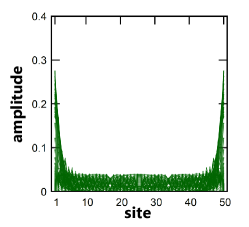
Figure S1: $\mathbb{Z}_{2}$ skin effect in a time-reversal-invariant topological insulator ($t=1.0$, $m=-1.6$, $\Delta=0.3$). The amplitude of the right eigenstates of the effective non-Hermitian Hamiltonian are shown.

References

• Hasan and Kane [2010] M. Z. Hasan and C. L. Kane, Colloquium: Topological insulators, Rev. Mod. Phys. 82, 3045 (2010).
• Qi and Zhang [2011] X.-L. Qi and S.-C. Zhang, Topological insulators and superconductors, Rev. Mod. Phys. 83, 1057 (2011).
• Altland and Zirnbauer [1997] A. Altland and M. R. Zirnbauer, Nonstandard symmetry classes in mesoscopic normal-superconducting hybrid structures, Phys. Rev. B 55, 1142 (1997).
• Schnyder et al. [2008] A. P. Schnyder, S. Ryu, A. Furusaki, and A. W. W. Ludwig, Classification of topological insulators and superconductors in three spatial dimensions, Phys. Rev. B 78, 195125 (2008).
• Ryu et al. [2010] S. Ryu, A. P. Schnyder, A. Furusaki, and A. W. W. Ludwig, Topological insulators and superconductors: tenfold way and dimensional hierarchy, New J. Phys. 12, 065010 (2010).
• Kitaev [2009] A. Kitaev, Periodic table for topological insulators and superconductors, AIP Conf. Proc. 1134, 22 (2009).
• Chiu et al. [2016] C.-K. Chiu, J. C. Y. Teo, A. P. Schnyder, and S. Ryu, Classification of topological quantum matter with symmetries, Rev. Mod. Phys. 88, 035005 (2016).
• Rudner and Levitov [2009] M. S. Rudner and L. S. Levitov, Topological Transition in a Non-Hermitian Quantum Walk, Phys. Rev. Lett. 102, 065703 (2009).
• Sato et al. [2012] M. Sato, K. Hasebe, K. Esaki, and M. Kohmoto, Time-Reversal Symmetry in Non-Hermitian Systems, Prog. Theor. Phys. 127, 937 (2012).
• Esaki et al. [2011] K. Esaki, M. Sato, K. Hasebe, and M. Kohmoto, Edge states and topological phases in non-Hermitian systems, Phys. Rev. B 84, 205128 (2011).
• Hu and Hughes [2011] Y. C. Hu and T. L. Hughes, Absence of topological insulator phases in non-Hermitian PT-symmetric Hamiltonians, Phys. Rev. B 84, 153101 (2011).
• Schomerus [2013] H. Schomerus, Topologically protected midgap states in complex photonic lattices, Opt. Lett. 38, 1912 (2013).
• Longhi et al. [2015] S. Longhi, D. Gatti, and G. D. Valle, Robust light transport in non-Hermitian photonic lattices, Sci. Rep. 5, 13376 (2015).
• Lee [2016] T. E. Lee, Anomalous Edge State in a Non-Hermitian Lattice, Phys. Rev. Lett. 116, 133903 (2016).
• Leykam et al. [2017] D. Leykam, K. Y. Bliokh, C. Huang, Y. D. Chong, and F. Nori, Edge Modes, Degeneracies, and Topological Numbers in Non-Hermitian Systems, Phys. Rev. Lett. 118, 040401 (2017).
• Xu et al. [2017] Y. Xu, S.-T. Wang, and L.-M. Duan, Weyl Exceptional Rings in a Three-Dimensional Dissipative Cold Atomic Gas, Phys. Rev. Lett. 118, 045701 (2017).
• Shen et al. [2018] H. Shen, B. Zhen, and L. Fu, Topological Band Theory for Non-Hermitian Hamiltonians, Phys. Rev. Lett. 120, 146402 (2018).
• Takata and Notomi [2018] K. Takata and M. Notomi, Photonic Topological Insulating Phase Induced Solely by Gain and Loss, Phys. Rev. Lett. 121, 213902 (2018).
• Martinez Alvarez et al. [2018] V. M. Martinez Alvarez, J. E. Barrios Vargas, and L. E. F. Foa Torres, Non-Hermitian robust edge states in one dimension: Anomalous localization and eigenspace condensation at exceptional points, Phys. Rev. B 97, 121401(R) (2018).
• Gong et al. [2018] Z. Gong, Y. Ashida, K. Kawabata, K. Takasan, S. Higashikawa, and M. Ueda, Topological Phases of Non-Hermitian Systems, Phys. Rev. X 8, 031079 (2018).
• Kawabata et al. [2019a] K. Kawabata, S. Higashikawa, Z. Gong, Y. Ashida, and M. Ueda, Topological unification of time-reversal and particle-hole symmetries in non-Hermitian physics, Nat. Commun. 10, 297 (2019a).
• Yao and Wang [2018] S. Yao and Z. Wang, Edge States and Topological Invariants of Non-Hermitian Systems, Phys. Rev. Lett. 121, 086803 (2018).
• Yao et al. [2018] S. Yao, F. Song, and Z. Wang, Non-Hermitian Chern Bands, Phys. Rev. Lett. 121, 136802 (2018).
• Kunst et al. [2018] F. K. Kunst, E. Edvardsson, J. C. Budich, and E. J. Bergholtz, Biorthogonal Bulk-Boundary Correspondence in Non-Hermitian Systems, Phys. Rev. Lett. 121, 026808 (2018).
• McDonald et al. [2018] A. McDonald, T. Pereg-Barnea, and A. A. Clerk, Phase-Dependent Chiral Transport and Effective Non-Hermitian Dynamics in a Bosonic Kitaev-Majorana Chain, Phys. Rev. X 8, 041031 (2018).
• Lee and Thomale [2019] C. H. Lee and R. Thomale, Anatomy of skin modes and topology in non-Hermitian systems, Phys. Rev. B 99, 201103(R) (2019).
• Liu et al. [2019] T. Liu, Y.-R. Zhang, Q. Ai, Z. Gong, K. Kawabata, M. Ueda, and F. Nori, Second-Order Topological Phases in Non-Hermitian Systems, Phys. Rev. Lett. 122, 076801 (2019).
• Lee et al. [2019a] C. H. Lee, L. Li, and J. Gong, Hybrid Higher-Order Skin-Topological Modes in Nonreciprocal Systems, Phys. Rev. Lett. 123, 016805 (2019a).
• Kawabata et al. [2019b] K. Kawabata, K. Shiozaki, M. Ueda, and M. Sato, Symmetry and Topology in Non-Hermitian Physics, Phys. Rev. X 9, 041015 (2019b).
• Zhou and Lee [2019] H. Zhou and J. Y. Lee, Periodic table for topological bands with non-Hermitian symmetries, Phys. Rev. B 99, 235112 (2019).
• Herviou et al. [2019] L. Herviou, J. H. Bardarson, and N. Regnault, Defining a bulk-edge correspondence for non-Hermitian Hamiltonians via singular-value decomposition, Phys. Rev. A 99, 052118 (2019).
• Zirnstein et al. [2021] H.-G. Zirnstein, G. Refael, and B. Rosenow, Bulk-Boundary Correspondence for Non-Hermitian Hamiltonians via Green Functions, Phys. Rev. Lett. 126, 216407 (2021).
• Borgnia et al. [2020] D. S. Borgnia, A. J. Kruchkov, and R.-J. Slager, Non-Hermitian Boundary Modes and Topology, Phys. Rev. Lett. 124, 056802 (2020).
• Yokomizo and Murakami [2019] K. Yokomizo and S. Murakami, Non-Bloch Band Theory of Non-Hermitian Systems, Phys. Rev. Lett. 123, 066404 (2019).
• Chang et al. [2020] P.-Y. Chang, J.-S. You, X. Wen, and S. Ryu, Entanglement spectrum and entropy in topological non-Hermitian systems and nonunitary conformal field theory, Phys. Rev. Research 2, 033069 (2020).
• Wanjura et al. [2020] C. C. Wanjura, M. Brunelli, and A. Nunnenkamp, Topological framework for directional amplification in driven-dissipative cavity arrays, Nat. Commun. 11, 3149 (2020).
• Zhang et al. [2020] K. Zhang, Z. Yang, and C. Fang, Correspondence between Winding Numbers and Skin Modes in Non-Hermitian Systems, Phys. Rev. Lett. 125, 126402 (2020).
• Okuma et al. [2020] N. Okuma, K. Kawabata, K. Shiozaki, and M. Sato, Topological Origin of Non-Hermitian Skin Effects, Phys. Rev. Lett. 124, 086801 (2020).
• Denner et al. [2021] M. M. Denner, A. Skurativska, F. Schindler, M. H. Fischer, R. Thomale, T. Bzdušek, and T. Neupert, Exceptional topological insulators, Nat. Commun. 12, 5681 (2021).
• Denner et al. [2023] M. M. Denner, T. Neupert, and F. Schindler, Infernal and exceptional edge modes: non-Hermitian topology beyond the skin effect, J. Phys. Mater. 6, 045006 (2023).
• Okugawa et al. [2020] R. Okugawa, R. Takahashi, and K. Yokomizo, Second-order topological non-Hermitian skin effects, Phys. Rev. B 102, 241202(R) (2020).
• Kawabata et al. [2020] K. Kawabata, M. Sato, and K. Shiozaki, Higher-order non-Hermitian skin effect, Phys. Rev. B 102, 205118 (2020).
• Fu et al. [2021] Y. Fu, J. Hu, and S. Wan, Non-Hermitian second-order skin and topological modes, Phys. Rev. B 103, 045420 (2021).
• Kawabata et al. [2021] K. Kawabata, K. Shiozaki, and S. Ryu, Topological Field Theory of Non-Hermitian Systems, Phys. Rev. Lett. 126, 216405 (2021).
• Zhang et al. [2022] K. Zhang, Z. Yang, and C. Fang, Universal non-Hermitian skin effect in two and higher dimensions, Nat. Commun. 13, 2496 (2022).
• Sun et al. [2021] X.-Q. Sun, P. Zhu, and T. L. Hughes, Geometric Response and Disclination-Induced Skin Effects in Non-Hermitian Systems, Phys. Rev. Lett. 127, 066401 (2021).
• Kim and Park [2021] K.-M. Kim and M. J. Park, Disorder-driven phase transition in the second-order non-Hermitian skin effect, Phys. Rev. B 104, L121101 (2021).
• Nakamura et al. [2024] D. Nakamura, T. Bessho, and M. Sato, Bulk-Boundary Correspondence in Point-Gap Topological Phases, Phys. Rev. Lett. 132, 136401 (2024).
• Wang et al. [2024] H.-Y. Wang, F. Song, and Z. Wang, Amoeba Formulation of Non-Bloch Band Theory in Arbitrary Dimensions, Phys. Rev. X 14, 021011 (2024).
• Nakai et al. [2024] Y. O. Nakai, N. Okuma, D. Nakamura, K. Shimomura, and M. Sato, Topological enhancement of nonnormality in non-Hermitian skin effects, Phys. Rev. B 109, 144203 (2024).
• Bergholtz et al. [2021] E. J. Bergholtz, J. C. Budich, and F. K. Kunst, Exceptional topology of non-Hermitian systems, Rev. Mod. Phys. 93, 015005 (2021).
• Okuma and Sato [2023] N. Okuma and M. Sato, Non-Hermitian Topological Phenomena: A Review, Annu. Rev. Condens. Matter Phys. 14, 83 (2023).
• Konotop et al. [2016] V. V. Konotop, J. Yang, and D. A. Zezyulin, Nonlinear waves in $\mathcal{PT}$-symmetric systems, Rev. Mod. Phys. 88, 035002 (2016).
• El-Ganainy et al. [2018] R. El-Ganainy, K. G. Makris, M. Khajavikhan, Z. H. Musslimani, S. Rotter, and D. N. Christodoulides, Non-Hermitian physics and PT symmetry, Nat. Phys. 14, 11 (2018).
• [55] V. Kozii and L. Fu, Non-Hermitian Topological Theory of Finite-Lifetime Quasiparticles: Prediction of Bulk Fermi Arc Due to Exceptional Point, arXiv:1708.05841 .
• Papaj et al. [2019] M. Papaj, H. Isobe, and L. Fu, Nodal arc of disordered Dirac fermions and non-Hermitian band theory, Phys. Rev. B 99, 201107 (2019).
• Shen and Fu [2018] H. Shen and L. Fu, Quantum Oscillation from In-Gap States and a Non-Hermitian Landau Level Problem, Phys. Rev. Lett. 121, 026403 (2018).
• Yoshida et al. [2018] T. Yoshida, R. Peters, and N. Kawakami, Non-Hermitian perspective of the band structure in heavy-fermion systems, Phys. Rev. B 98, 035141 (2018).
• Hirsbrunner et al. [2019] M. R. Hirsbrunner, T. M. Philip, and M. J. Gilbert, Topology and observables of the non-Hermitian Chern insulator, Phys. Rev. B 100, 081104(R) (2019).
• McClarty and Rau [2019] P. A. McClarty and J. G. Rau, Non-Hermitian topology of spontaneous magnon decay, Phys. Rev. B 100, 100405(R) (2019).
• Bergholtz and Budich [2019] E. J. Bergholtz and J. C. Budich, Non-Hermitian Weyl physics in topological insulator ferromagnet junctions, Phys. Rev. Research 1, 012003(R) (2019).
• Michishita and Peters [2020] Y. Michishita and R. Peters, Equivalence of Effective Non-Hermitian Hamiltonians in the Context of Open Quantum Systems and Strongly Correlated Electron Systems, Phys. Rev. Lett. 124, 196401 (2020).
• Okuma and Sato [2021] N. Okuma and M. Sato, Non-Hermitian Skin Effects in Hermitian Correlated or Disordered Systems: Quantities Sensitive or Insensitive to Boundary Effects and Pseudo-Quantum-Number, Phys. Rev. Lett. 126, 176601 (2021).
• Lehmann et al. [2021] C. Lehmann, M. Schüler, and J. C. Budich, Dynamically Induced Exceptional Phases in Quenched Interacting Semimetals, Phys. Rev. Lett. 127, 106601 (2021).
• [65] J. Cayao and M. Sato, Non-Hermitian phase-biased Josephson junctions, arXiv:2307.15472 .
• Poli et al. [2015] C. Poli, M. Bellec, U. Kuhl, F. Mortessagne, and H. Schomerus, Selective enhancement of topologically induced interface states in a dielectric resonator chain, Nat. Commun. 6, 6710 (2015).
• Zeuner et al. [2015] J. M. Zeuner, M. C. Rechtsman, Y. Plotnik, Y. Lumer, S. Nolte, M. S. Rudner, M. Segev, and A. Szameit, Observation of a Topological Transition in the Bulk of a Non-Hermitian System, Phys. Rev. Lett. 115, 040402 (2015).
• Zhen et al. [2015] B. Zhen, C. W. Hsu, Y. Igarashi, L. Lu, I. Kaminer, A. Pick, S.-L. Chua, J. D. Joannopoulos, and M. Soljac̆ić, Spawning rings of exceptional points out of Dirac cones, Nature 525, 354 (2015).
• Weimann et al. [2017] S. Weimann, M. Kremer, Y. Plotnik, Y. Lumer, S. Nolte, K. G. Makris, M. Segev, M. C. Rechtsman, and A. Szameit, Topologically protected bound states in photonic parity-time-symmetric crystals, Nat. Mater. 16, 433 (2017).
• Xiao et al. [2017] L. Xiao, X. Zhan, Z. H. Bian, K. K. Wang, X. Zhang, X. P. Wang, J. Li, K. Mochizuki, D. Kim, N. Kawakami, W. Yi, H. Obuse, B. C. Sanders, and P. Xue, Observation of topological edge states in parity-time-symmetric quantum walks, Nat. Phys. 13, 1117 (2017).
• St-Jean et al. [2017] P. St-Jean, V. Goblot, E. Galopin, A. Lemaître, T. Ozawa, L. L. Gratiet, I. Sagnes, J. Bloch, and A. Amo, Lasing in topological edge states of a one-dimensional lattice, Nat. Photon. 11, 651 (2017).
• Parto et al. [2018] M. Parto, S. Wittek, H. Hodaei, G. Harari, M. A. Bandres, J. Ren, M. C. Rechtsman, M. Segev, D. N. Christodoulides, and M. Khajavikhan, Edge-Mode Lasing in 1D Topological Active Arrays, Phys. Rev. Lett. 120, 113901 (2018).
• Bahari et al. [2017] B. Bahari, A. Ndao, F. Vallini, A. E. Amili, Y. Fainman, and B. Kanté, Nonreciprocal lasing in topological cavities of arbitrary geometries, Science 358, 636 (2017).
• Zhao et al. [2018] H. Zhao, P. Miao, M. H. Teimourpour, S. Malzard, R. El-Ganainy, H. Schomerus, and L. Feng, Topological hybrid silicon microlasers, Nat. Commun. 9, 981 (2018).
• Zhou et al. [2018] H. Zhou, C. Peng, Y. Yoon, C. W. Hsu, K. A. Nelson, L. Fu, J. D. Joannopoulos, M. Soljac̆ić, and B. Zhen, Observation of bulk Fermi arc and polarization half charge from paired exceptional points, Science 359, 1009 (2018).
• Harari et al. [2018] G. Harari, M. A. Bandres, Y. Lumer, M. C. Rechtsman, Y. D. Chong, M. Khajavikhan, D. N. Christodoulides, and M. Segev, Topological insulator laser: Theory, Science 359, eaar4003 (2018).
• Bandres et al. [2018] M. A. Bandres, S. Wittek, G. Harari, M. Parto, J. Ren, M. Segev, D. Christodoulides, and M. Khajavikhan, Topological insulator laser: Experiments, Science 359, eaar4005 (2018).
• Cerjan et al. [2019] A. Cerjan, S. Huang, K. P. Chen, Y. Chong, and M. C. Rechtsman, Experimental realization of a Weyl exceptional ring, Nat. Photon. 13, 623 (2019).
• Zhao et al. [2019] H. Zhao, X. Qiao, T. Wu, B. Midya, S. Longhi, and L. Feng, Non-Hermitian topological light steering, Science 365, 1163 (2019).
• Brandenbourger et al. [2019] M. Brandenbourger, X. Locsin, E. Lerner, and C. Coulais, Non-reciprocal robotic metamaterials, Nat. Commun. 10, 4608 (2019).
• Ghatak et al. [2020] A. Ghatak, M. Brandenbourger, J. van Wezel, and C. Coulais, Observation of non-Hermitian topology and its bulk-edge correspondence in an active mechanical metamaterial, Proc. Natl. Acad. Sci. USA 117, 29561 (2020).
• Helbig et al. [2020] T. Helbig, T. Hofmann, S. Imhof, M. Abdelghany, T. Kiessling, L. W. Molenkamp, C. H. Lee, A. Szameit, M. Greiter, and R. Thomale, Generalized bulk-boundary correspondence in non-Hermitian topolectrical circuits, Nat. Phys. 16, 747 (2020).
• Hofmann et al. [2020] T. Hofmann, T. Helbig, F. Schindler, N. Salgo, M. Brzezińska, M. Greiter, T. Kiessling, D. Wolf, A. Vollhardt, A. Kabaši, C. H. Lee, A. Bilušić, R. Thomale, and T. Neupert, Reciprocal skin effect and its realization in a topolectrical circuit, Phys. Rev. Research 2, 023265 (2020).
• Xiao et al. [2020] L. Xiao, T. Deng, K. Wang, G. Zhu, Z. Wang, W. Yi, and P. Xue, Non-Hermitian bulk-boundary correspondence in quantum dynamics, Nat. Phys. 16, 761 (2020).
• Weidemann et al. [2020] S. Weidemann, M. Kremer, T. Helbig, T. Hofmann, A. Stegmaier, M. Greiter, R. Thomale, and A. Szameit, Topological funneling of light, Science 368, 311 (2020).
• Gou et al. [2020] W. Gou, T. Chen, D. Xie, T. Xiao, T.-S. Deng, B. Gadway, W. Yi, and B. Yan, Tunable Nonreciprocal Quantum Transport through a Dissipative Aharonov-Bohm Ring in Ultracold Atoms, Phys. Rev. Lett. 124, 070402 (2020).
• Liang et al. [2022] Q. Liang, D. Xie, Z. Dong, H. Li, H. Li, B. Gadway, W. Yi, and B. Yan, Dynamic Signatures of Non-Hermitian Skin Effect and Topology in Ultracold Atoms, Phys. Rev. Lett. 129, 070401 (2022).
• Palacios et al. [2020] L. S. Palacios, S. Tchoumakov, M. Guix, I. P. S. Sánchez, and A. G. Grushin, Guided accumulation of active particles by topological design of a second-order skin effect, Nat. Commun. 12, 4691 (2020).
• Zhang et al. [2021] X. Zhang, Y. Tian, J.-H. Jiang, M.-H. Lu, and Y.-F. Chen, Observation of higher-order non-Hermitian skin effect, Nat. Commun. 12, 5377 (2021).
• Wang et al. [2023] A. Wang, Z. Meng, and C. Q. Chen, Non-Hermitian topology in static mechanical metamaterials, Sci. Adv. 9, eadf7299 (2023).
• [91] R. Shen, T. Chen, B. Yang, and C. H. Lee, Observation of the non-Hermitian skin effect and Fermi skin on a digital quantum computer, arXiv:2311.10143 .
• Lee et al. [2019b] J. Y. Lee, J. Ahn, H. Zhou, and A. Vishwanath, Topological Correspondence between Hermitian and Non-Hermitian Systems: Anomalous Dynamics, Phys. Rev. Lett. 123, 206404 (2019b).
• Bessho and Sato [2021] T. Bessho and M. Sato, Nielsen-Ninomiya Theorem with Bulk Topology: Duality in Floquet and Non-Hermitian Systems, Phys. Rev. Lett. 127, 196404 (2021).
• Li et al. [2022] Y. Li, C. Liang, C. Wang, C. Lu, and Y.-C. Liu, Gain-Loss-Induced Hybrid Skin-Topological Effect, Phys. Rev. Lett. 128, 223903 (2022).
• Zhu and Gong [2022] W. Zhu and J. Gong, Hybrid skin-topological modes without asymmetric couplings, Phys. Rev. B 106, 035425 (2022).
• Zhu and Gong [2023] W. Zhu and J. Gong, Photonic corner skin modes in non-Hermitian photonic crystals, Phys. Rev. B 108, 035406 (2023).
• Ou et al. [2023] Z. Ou, Y. Wang, and L. Li, Non-Hermitian boundary spectral winding, Phys. Rev. B 107, L161404 (2023).
• Ma et al. [2024] X.-R. Ma, K. Cao, X.-R. Wang, Z. Wei, Q. Du, and S.-P. Kou, Non-Hermitian chiral skin effect, Phys. Rev. Research 6, 013213 (2024).
• Schindler et al. [2023] F. Schindler, K. Gu, B. Lian, and K. Kawabata, Hermitian Bulk – Non-Hermitian Boundary Correspondence, PRX Quantum 4, 030315 (2023).
• Nakamura et al. [2023] D. Nakamura, K. Inaka, N. Okuma, and M. Sato, Universal Platform of Point-Gap Topological Phases from Topological Materials, Phys. Rev. Lett. 131, 256602 (2023).
• Liu et al. [2024] G.-G. Liu, S. Mandal, P. Zhou, X. Xi, R. Banerjee, Y.-H. Hu, M. Wei, M. Wang, Q. Wang, Z. Gao, H. Chen, Y. Yang, Y. Chong, and B. Zhang, Localization of Chiral Edge States by the Non-Hermitian Skin Effect, Phys. Rev. Lett. 132, 113802 (2024).
• [102] J. Wu, R. Zheng, J. Liang, M. Ke, J. Lu, W. Deng, X. Huang, and Z. Liu, Spin-dependent localization of helical edge states in a non-Hermitian phononic crystal, arXiv:2312.12060 .
• Datta [1995] S. Datta, Electronic Transport in Mesoscopic Systems (Cambridge University Press, Cambridge, England, 1995).
• Moiseyev [2011] N. Moiseyev, Non-Hermitian Quantum Mechanics (Cambridge University Press, Cambridge, England, 2011).
• [105] See the Supplemental Material, which includes Refs. [122, 123, 124, 121, 125], for details on effective non-Hermitian Hamiltonians, symmetry classification of non-Hermitian self-energy, analytical derivations of self-energy, current formulas, and $\mathbb{Z}_{2}$ skin effect in time-reversal-invariant topological insulators.
• Hatano and Nelson [1996] N. Hatano and D. R. Nelson, Localization Transitions in Non-Hermitian Quantum Mechanics, Phys. Rev. Lett. 77, 570 (1996).
• Hatano and Nelson [1997] N. Hatano and D. R. Nelson, Vortex pinning and non-Hermitian quantum mechanics, Phys. Rev. B 56, 8651 (1997).
• Hatano [2021] N. Hatano, What is the resonant state in open quantum systems?, J. Phys.: Conf. Ser. 2038, 012013 (2021).
• Su et al. [1979] W. P. Su, J. R. Schrieffer, and A. J. Heeger, Solitons in Polyacetylene, Phys. Rev. Lett. 42, 1698 (1979).
• [110] $\eta=1/\sqrt{L}$ is chosen to be much larger than the level spacing $\sim 1/L$ but much smaller than the macroscopic energy scale $\sim 1$.
• Qi et al. [2006] X.-L. Qi, Y.-S. Wu, and S.-C. Zhang, Topological quantization of the spin Hall effect in two-dimensional paramagnetic semiconductors, Phys. Rev. B 74, 085308 (2006).
• Qi et al. [2008] X.-L. Qi, T. L. Hughes, and S.-C. Zhang, Topological field theory of time-reversal invariant insulators, Phys. Rev. B 78, 195424 (2008).
• Datta [2005] S. Datta, Quantum Transport (Cambridge University Press, Cambridge, England, 2005).
• Bernevig et al. [2006] B. A. Bernevig, T. L. Hughes, and S.-C. Zhang, Quantum Spin Hall Effect and Topological Phase Transition in HgTe Quantum Wells, Science 314, 1757 (2006).
• Eek et al. [2024] L. Eek, A. Moustaj, M. Röntgen, V. Pagneux, V. Achilleos, and C. M. Smith, Emergent non-Hermitian models, Phys. Rev. B 109, 045122 (2024).
• Franca et al. [2022] S. Franca, V. Könye, F. Hassler, J. van den Brink, and C. Fulga, Non-Hermitian Physics without Gain or Loss: The Skin Effect of Reflected Waves, Phys. Rev. Lett. 129, 086601 (2022).
• Ochkan et al. [2024] K. Ochkan, R. Chaturvedi, V. Könye, L. Veyrat, R. Giraud, D. Mailly, A. Cavanna, U. Gennser, E. M. Hankiewicz, B. Büchner, J. van den Brink, J. Dufouleur, and I. C. Fulga, Non-Hermitian topology in a multi-terminal quantum Hall device, Nat. Phys. 20, 395 (2024).
• Fujikawa and Suzuki [2004] K. Fujikawa and H. Suzuki, Path Integrals and Quantum Anomalies (Oxford University Press, Oxford, 2004).
• Karsten [1981] L. H. Karsten, Lattice fermions in euclidean space-time, Phys. Lett. B 104, 315 (1981).
• Chen et al. [2023] W.-Q. Chen, Y.-S. Wu, W. Xi, W.-Z. Yi, and G. Yue, Fate of Quantum Anomalies for 1d lattice chiral fermion with a simple non-Hermitian Hamiltonian, J. High Energ. Phys. 2023 (5), 90.
• Sirker et al. [2014] J. Sirker, M. Maiti, N. P. Konstantinidis, and N. Sedlmayr, Boundary fidelity and entanglement in the symmetry protected topological phase of the SSH model, J. Stat. Mech. 2014, P10032 (2014).
• Ryndyk et al. [2009] D. A. Ryndyk, R. Gutiérrez, B. Song, and G. Cuniberti, Green Function Techniques in the Treatment of Quantum Transport at the Molecular Scale, in Energy Transfer Dynamics in Biomaterial Systems, edited by I. Burghardt, V. May, D. A. Micha, and E. R. Bittner (Springer, Berlin, Heidelberg, 2009) pp. 213–335.
• Lieu et al. [2020] S. Lieu, M. McGinley, and N. R. Cooper, Tenfold Way for Quadratic Lindbladians, Phys. Rev. Lett. 124, 040401 (2020).
• Kawabata et al. [2023] K. Kawabata, Z. Xiao, T. Ohtsuki, and R. Shindou, Singular-Value Statistics of Non-Hermitian Random Matrices and Open Quantum Systems, PRX Quantum 4, 040312 (2023).
• Shin [1997] B. C. Shin, A formula for Eigenpairs of certain symmetric tridiagonal matrices, Bull. Aust. Math. Soc. 55, 249 (1997).