The Instrumental Variable Model with Categorical Instrument, Treatment and Outcome

1 Introduction: Instrumental Variable Model and Motivating Example

1.1 Instrumental Variable Model

Instrumental variable (IV) analysis is a crucial tool in statistical analysis. They help in estimating causal relationships by addressing the issue of confounding variables that may bias the results. Instrumental variable analysis can be used to draw causal conclusions in observational studies if random experiments are impractical or infeasible. Recent work on Mendelian Randomization is a type of IV analysis with genetic variants as instrumental variables [4, 6, 14]. IV analysis could also help in addressing other aspects of designed randomized experiments including clinical trials with non-compliance.

Let $X$ and $Y$ denote the exposure and outcome of interest respectively. Generally speaking, a variable $Z$ is a valid instrumental variable if the following assumptions hold.

1. Relevance condition: $Z$ is associated with the exposure $X$. This assumption allows $Z$ to serve as a valid proxy of the exposure $X$.

2. Independence condition: $Z$ is independent of any unmeasured confounder of the exposure-outcome relationship

3. Exclusion restriction: There is no direct effect of $Z$ on the outcome $Y$ that is not fully through the exposure of interest $X$

Variations of the independence assumption above will be discussed later in the paper. A directed acyclic graph (DAG) representing the assumptions on instrumental variables is shown in Figure 1.

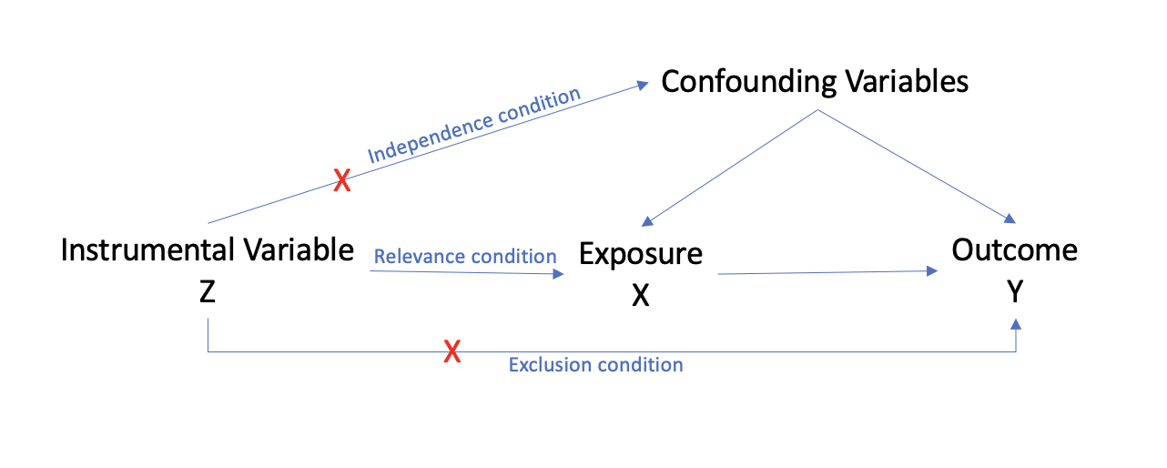
Figure 1: Directed acyclic graph (DAG) representing the assumptions of a valid instrumental variable

1.2 Previous Results and Our Contribution

In instrumental variable analysis, the counterfactual distributions of $Y$ (or the average treatment effect (ATE)) cannot be point-identified in general without additional assumptions. It is often of interest to obtain bounds using the observed probability distributions of $P(X,Y\mid Z)$ which is referred to as partial identification in the literature. A large proportion of the literature focuses on binary exposure and outcome, while situations of categorical exposure and outcome with more than 2 levels are less explored. For example, [1] developed bounds on average treatment effect for binary IV models where $Z,X,Y$ are all binary. Furthermore, Richardson and Robins showed under individual-level exclusion restriction $Y(x)=Y(x,z)$ and all variations of independence condition presented later, the joint probability distribution of the potential outcomes $P(Y(x_{1}),Y(x_{2}))$ is characterized by the inequalities when $X,Y$ are binary and $Z$ has $Q$ states. For $i\in\{1,2\}$, $y\in\{1,2\}$, $\tilde{y}\in\{1,2\}$ and $z\in\{1,\ldots,Q\}$, we have

$$P(Y(x_{i})=y) \leq P(Y=y;X=i\mid Z=z)+P(X=3-i\mid Z=z)$$ (1)

$$P(Y(x_{1})=y;Y(x_{2})=\tilde{y}) \leq P(Y=y;X=1\mid Z=z)+P(Y=\tilde{y};X=2\mid Z=z)$$ (2)

There are $4Q$ pairs of inequalities since there are 4 combinations of $x_{i}$ and $y$ in inequality (1) and 4 combinations of $y$ and $\tilde{y}$ in inequality (2) given each of the $Q$ states of $Z$.

Regarding work on IV model beyond binary treatment and outcome, [3] and [8] derived generalized instrumental inequalities for falsification of the instrumental variable independence assumption, while these bounds are not sufficient in characterizing the counterfactual probability distributions. [5] worked on the estimation of ATE in a three-arm trial with non-compliance but with the assumption of the monotonicity of compliance. [2] studied partial identification using random set theory and introduced a novel framework for addressing identification challenges in econometric models. However, the practical implementation of random set theory may require substantial computational resources, limiting its applicability in certain settings. Further, the framework was studied under the joint statistical independence assumption which is a less restrictive model than random assignment. [13] proposed a procedure to estimate the bounds on functionals of the joint distribution of the counterfactual probability distributions without closed-form expressions for bounds on functions of the joint distribution while noting that they can be difficult to derive ([10]).

Our paper provides a simple characterization of the joint counterfactual probability distribution when the instrument, exposure, and outcome are discrete and take finite states. The bounds we derived are sufficient, necessary, and non-redundant, and we argue that these results offer valuable insights into the understanding of the fundamentals of IV models and aid computational developments of statistical inference. We further explore the violation of variation independence property of the marginal counterfactual probabilities which has direct implications of estimands of interest such as paired contrasts of $P(Y(x_{i})=y)$ and $P(Y(x_{j})=y)$ where $i\neq j$, i.e. the average treatment effect (ATE).

1.3 Motivating Example: Caution!

Let’s consider a clinical trial of alcohol use dependency (AUD) with three arms. Patients are randomly assigned to either a control arm or one of two treatment arms. The control arm is simple medication management, while the two treatment arms have either (1) compliance enhancement therapy or (2) cognitive behavioral therapy concurrently with simple medication management. Compliance enhancement therapists educate patients on the treatment and motivate them to improve compliance with their medications as well as routine clinic visits. During cognitive behavior therapy, patients are educated on how to better deal with situations that lead to a higher risk of relapse in drinking. The outcome of interest is the relapse of drinking during the past month which is defined as having 5 drinks or more on any day. Patients assigned to the control arm do not have access to any of the therapies in the treatment arm, and patients assigned to one of the treatments do not have access to the other (while they can still switch to the control arm). Researchers are interested in estimating the average causal effect of treatment 1 compared to the control arm in this three-arm trial with non-compliance. We denote the assignment of the control, treatment 1, or treatment 2 arms as $Z=1,Z=2,Z=3$, and the actual treatment taken by the patients as $X=1,X=2,X=3$ respectively. We denote relapse during the first month as $Y=2$ while non-relapse as $Y=1$. We observe the following table.

Table 1: The alcohol use dependency trial data presented in [5]. The data in the red cells were not relevant to the research question of interest which the researchers want to estimate the average causal effect of treatment arm $X=2$ compared to the control arm $X=1$.

	X=1, Y=1	X=1, Y=2	X=2, Y=1	X=2, Y=2	X=3, Y=1	X=3, Y=2
Z=1	19	28	0	0	0	0
Z=2	8	7	14	21	0	0
Z=3	6	15	0	0	3	20

Consider the hypothetical (and hopefully not real!) situation in which the researchers are interested in estimating the average causal effect of treatment 1 compared to the control and thought treatment 2 was not their question of interest. In addition, they thought that problems with binary treatment and outcome are well-studied and easy to analyze. Therefore, they threw away all data with treatment 2 and proceeded with using the bounds shown in 1.2.

[17] showed that performing an IV analysis only using a subset of people who are assigned to their treatment arms of interest and ignoring other possible assignment options may lead to biased results. Conceptually, this is wrong because (1) we are throwing out people with certain potential subtypes so that the estimand is also changed and restricted to the average treatment effect for the population without those subtypes. In our case, deleting data on treatment arm $X=3$ means we ignore compliers who would take treatment 2 if they were assigned to it. This is no longer a proper causal estimand; (2) there might be additional constraints on the counterfactual probability distributions of $P(Y(x_{1}))$ and $P(Y(x_{2}))$ when we have an additional arm $X=3$ with $P(Y(x_{3}))$ being non-zero.

1.4 Outline

After introducing notations and assumptions in Section 2.1, we present our main results on the characterization of the joint probability distribution of the potential outcomes in Section 2.2, followed by an illustration of how to re-derive the bounds presented in Section 1.2 using Strassen’s theorem. In Section 3, we discuss the variation (in)dependence property of the marginal probability distribution of the potential outcomes $P(Y(x_{i}))$. Section 4 presents simulation results on how likely we reject the IV model if the data is generated under uniform Dirichlet distribution. We finish the paper with a summary in Section 5.

2 Notation and Main Theorems

2.1 Basic Notations and Assumptions

Consider a categorical outcome $Y$ with $M$ levels, an exposure variable $X$ with $K$ levels, and an instrumental variable $Z$ with $Q$ levels, where each variable takes values from $\{1,\dots,M\}$, $\{1,\dots,K\}$, and $\{1,\dots,Q\}$ respectively, with $M,K,Q\geq 2$. We use $X(z_{q})$ to denote $X(Z=q)$, $q=1,\ldots,Q$.

First, we discuss the key assumptions under which our results are developed.

Assumption 1 (Individual-level Exclusion Restriction).

$$Y(X=x)=Y(X=x,Z=z)\text{ for all }x\in\{1,\dots,K\}\text{ and }z\in\{1,\dots,Q\}$$

We denote the $K$ potential outcomes for $Y$ as $Y(x_{1}),\ldots,Y(x_{K})$.

In the literature, variations of the independence assumptions are considered under different methods and areas [16]. Our results hold under any of the independence conditions listed below.

Assumption 2 (Variations of Independence Condition).

Variations of the independence assumptions in the literature:

1. Random Assignment: $Z\perp Y(x_{1}),\dots,Y(x_{K}),X(z_{1}),\dots,X(z_{Q})$

2. Joint Exogeneity: $Z\perp Y(x_{1}),\dots,Y(x_{K})$

3. Marginal Exogeneity: for $q\in\{1,\dots,Q\}$, $i\in\{1,\dots,K\}$, $Z\perp X(z_{q}),Y(x_{i})$

4. Latent-Variable Marginal Exogeneity: there exists $U$ such that $U\perp Z$ and for $i\in\{1,\ \dots,K\}$, $Y(x_{i})\perp X,Z\mid U$

Note that the relevance assumption only comes into play with whether the bound derived is informative or not, but it is not useful for other aspects of partial identification.

Let ${\cal A}$ be the sample space of events $\{(X=i,Y(x_{i})=y)=\mathbf{w}:i=1,\ldots,K,y=1,\dots,M\}$, and ${\cal B}$ be the sample space of events $\{(Y({x_{1}}),\ldots,Y({x_{K})})=\mathbf{v}:\mathbf{v}\in\{1,\dots,M\}^{K}\}$. Notice that $\cal B$ is isomorphic to $\{1,\dots,M\}^{K}$, so we will denote ${\cal B}=\{1,\dots,M\}^{K}$ for the simplicity of notation. For example, we will use $\{(1,1,1)\}$ to denote the event in $\cal B$ $\{(Y(x_{1})=1,Y(x_{2})=1,Y(x_{3})=1)\}$. It is obvious that $|{\cal A}|=MK$ and $|{\cal B}|=M^{K}$. Let $\mathfrak{A}=2^{\cal A}$ and $\mathfrak{B}=2^{\cal B}$ be the power sets of $\cal A$ and $\cal B$. Let $P$, which is the conditional probability of $(X=x,Y(x)=y)$ given $Z=z$, be the probability measure on ${\cal A}$. Let $P^{\prime}$, which is the joint counterfactual probability of $(Y(x_{1}),\dots,Y(x_{K}))$, be the probability measure on ${\cal B}$.

Let ${\cal V}=\{v_{1},\dots,v_{a}\}\in{\mathfrak{B}}$ where $|{\cal V}|=a$ and $a=1,\dots,M^{K}$, and $v_{s}=(v_{s}^{(1)},\ldots,v_{s}^{(K)})\in\{1,\dots,M\}^{K}$, for $s=1,\ldots,a$. Define the extension of $\cal{V}$ as

$$\begin{split}ext(\mathcal{V})=\{l=(l^{(1)},\ldots,l^{(K)})\in\{1,\dots,M\}^{K}:\forall r\in\{1,\ldots K\},\\ \exists s\in\{1,\ldots,a\}\text{ s.t. }l^{(r)}=v_{s}^{(r)}\},\end{split}$$

and $|ext(\mathcal{V})|=2^{r}$ for some $r=1,\ldots,K$. Notice that $ext(\mathcal{V})$ is a matrix with $2^{r}$ rows and $K$ columns, and we will use $ext(\mathcal{V})_{i\cdot}\in\{1,\dots,M\}^{K}$ to denote the i-th row in $ext(\mathcal{V})$ and $ext(\mathcal{V})_{\cdot j}\in\{1,\dots,M\}^{|ext(\mathcal{V})|}$ to denote the j-th column in $ext(\mathcal{V})$.

Now, we define $Uniq(ext(\mathcal{V})_{\cdot j})\subseteq\{1,\dots,M\}$ to be a vector of all unique values in $ext(\mathcal{V})_{\cdot j}$. Given ${\mathcal{M}}\subseteq\{1,\dots,M\}$ and ${\mathcal{M}}\neq\emptyset$, we define

$$\Phi(ext({\mathcal{V}})),{\mathcal{M}})=\{j\in\{1,\dots,K\}\ s.t.\ {\mathcal{M}}=Uniq(ext(\mathcal{V})_{\cdot j})\},$$

which defines a partition of $\{1,\ldots,K\}$. That is, $\{1,\dots,K\}=\bigcup_{{\mathcal{M}}\subseteq\{1,\dots,M\}}\Phi(ext({\cal V}),{\mathcal{M}})$.

Example 1.

If $K=M=3$ and ${\cal V}=\begin{Bmatrix}1&2&1\\ 1&1&2\end{Bmatrix}$, then we have

$$ext(\mathcal{V})=\begin{Bmatrix}1&2&1\\ 1&1&2\\ 1&1&1\\ 1&2&2\end{Bmatrix}.$$

Further, let ${\cal M}_{1}=\{1\},{\cal M}_{2}=\{1,2\}$ and ${\cal M}_{3}=\{1,2,3\}$. Then, we have $\Phi(ext({\cal V}),{\mathcal{M}}_{1})={1},\Phi(ext({\cal V}),{\mathcal{M}}_{2})={2,3}$ and $\Phi(ext({\cal V}),{\mathcal{M}}_{3})=\emptyset$.

2.2 Main Results

We list the main results. The first is a characterization of the joint counterfactual distribution.

Theorem 1.

Under assumption 1 and any of the variations of the independence conditions stated in assumption 2, the joint counterfactual probability distribution $P^{\prime}(Y(x_{1}),\dots,Y(x_{K}))$ is characterized by the inequalities of form:

$$P^{\prime}(ext({\cal V}))\leq\sum_{{\cal M}\subseteq\{1,\dots,M\}}P(Y\in{\cal M},X\in\Phi(ext({\cal V}),{\cal M})\mid Z=z),\ \forall{\cal V}\in\mathfrak{B}$$ (3)

Some of the above inequalities may be implied by the other, and thus redundant. Let $C=\Phi(ext({\cal V}),\{1,\dots,M\})$. The following results find the redundant inequalities.

Proposition 1.

For the inequalities in the form of (3), it is redundant if and only if :

1. $|C|=K-1$, and

2. $|Uniq(ext(\mathcal{V})_{\cdot(\{1,\dots K\}\setminus C)})|<M-1$,
   or in other words,
   $\Phi(ext({\cal V}),{\mathcal{M}})=\emptyset$, $\forall{\mathcal{M}}\subseteq\{1,\dots,M\}$ and $|{\mathcal{M}}|=M-1,$

and there are $Q(K(2^{M}-M-2))$ of those redundant inequalities.

Proposition 2.

The number of non-trivial and non-redundant constraints in the form of (3) is $Q((2^{M}-1)^{K}-K(2^{M}-M-2)-1)$.

The following Lemma implies that we can consider each level of $Z=z\in\{1,\dots,Q\}$ separately.

Lemma 1.

Given a set of $q$ distributions $P_{z}(X(z),Y(x=1),\dots,Y(x=K))$, for $z\in\{1,\dots,Q\}$ that agree on the common marginals so that $P_{z}(Y(x=1),\dots Y(x=K))=P_{z*}(Y(x=1),\dots Y(x=K))$ for all $z,z*$, then there exists a single joint distribution:

$$P^{*}(X(z=1),\dots,X(z=Q),Y(x=1),\dots,Y(x=K))$$

that agrees with each of these $q$ marginals so that for all $Z=z$,

$$P_{z}(X(z),Y(x=1),\dots,Y(x=K))=P(X(z),Y(x=1),\dots,Y(x=K))$$

2.3 Strassen’s Theorem and applications

Strassen’s theorem is a fundamental result in probability theory. While the full technical statement of the theorem can be quite complex, involving detailed mathematical notations and conditions, it essentially provides necessary and sufficient conditions on the existence of a probability measure on two product spaces with given support and two marginals [15, 7]. Koperberg [9] stated a simplified version of Strassen’s theorem for finite sets. We restate their results below.

Definition 1.

Let ${\cal A}$ and ${\cal B}$ be sets and ${\cal R}\subseteq{\cal A}\times{\cal B}$ a relation. Then for each $U\subseteq{\cal A}$, the set of neighbors of $U$ in ${\cal R}$ is denoted by

$${\cal N}_{\cal R}(U)=\{\mathbf{v}\in{\cal B}:(U\times\{\mathbf{v}\})\cap{\cal R}\neq\emptyset\}$$

Strassen’s theorem for finite sets (Koperberg, 2024): Let ${\cal A}$ and ${\cal B}$ be finite sets, $P$ and $P^{\prime}$ probability measures on ${\cal A}$ and ${\cal B}$ respectively and ${\cal R}\subseteq{\cal A}\times{\cal B}$ a relation. Then, there exists a coupling $\hat{P}$ of $P$ and $P^{\prime}$ that satisfies $\hat{P}({\cal R})=1$ if and only if

$$P(U)\leq P^{\prime}({\cal N}_{\cal R}(U)),\text{ for all }U\subseteq{\cal A}.$$

For the proof of this theorem, refer to [9]. To utilize this result, $\mathcal{A}$ and $\mathcal{B}$ are the sample space of events we defined. We then define the following relation: given two outcomes $\mathbf{w}\in{\cal A}$ and $\mathbf{v}\in{\cal B}$ we will say that $\mathbf{w}$ and $\mathbf{v}$ are coherent if they assign the same values to any variables that are in common. Thus for example, $(X=1,Y(x_{1})=1)$ and $(Y(x_{1})=1,Y(x_{2})=1)$ are coherent, but $(X=1,Y(x_{1})=1)$ and $(Y(x_{1})=2,Y(x_{2})=1)$ are not.

Let

$${\mathfrak{C}}\equiv\{(\mathbf{w},\mathbf{v})\mid\mathbf{w}\in{\cal A},\mathbf{v}\in{\cal B},\mathbf{w}\hbox{ and }\mathbf{v}\hbox{ are coherent}\}\subseteq{\cal A}\times{\cal B}.$$ (4)

We may also view ${\mathfrak{C}}$ as specifying a set of edges in a bipartite graph; see Figure 2 for binary exposure and outcome. Notice that if $(\mathbf{w},\mathbf{v})\in{\mathfrak{C}}$, then the conjunction of $\mathbf{w}$ and $\mathbf{v}$ corresponds to an assignment to all three variables $(X,Y(x_{1}),Y(x_{2}))$ given $Z=z$; see Figure 3.

The bipartite graph $\mathcal{G}$ illustrating pairs of $(\mathbf{w},\mathbf{v})\in{\cal A}\times{\cal B}$ that are coherent like Figure 2 can be easily generalized. Each of the $MK$ elements in $\cal A$ is connected to $M^{K-1}$ elements in $\cal B$, while each of the $M^{K}$ elements in $\cal B$ is connected to $K$ elements in $\cal A$. The total number of edges in $\mathcal{G}$ is $KM^{K}$. We use $\mathcal{G}_{\cal V}$ to denote the subgraph of $\mathcal{G}$ that only includes edges connecting ${\cal V}\in{\mathfrak{B}}$ and ${\cal N}_{\mathfrak{C}}({\cal V})$. Note that the neighborhood of any event $\cal{V}\in\mathfrak{B}$, ${\cal N}_{\mathfrak{C}}({\cal V})$, contains at least one of the $K$ observed events for each level of $X$ in ${\cal A}$.

Strassen’s Theorem is a key in our proof of Theorem 1. In this section, we give an illustration of how Strassen’s theorem may be applied to prove the sufficiency of the inequalities defining the counterfactual probability distribution when $X$ and $Y$ are binary, i.e. bounds in the form of (1) and (2) (Step 3 in [11]’s proof). In the proof below, we have binary $X$ and $Y$ taking states $\{1,2\}$.

Consider the following sets, each containing four outcomes:

$${\cal A} =\left\{(X=1,Y(x_{1})=1),(X=1,Y(x_{1})=2),\right.$$

$$\kern 20.0pt\left.(X=2,Y(x_{2})=1),(X=2,Y(x_{2})=2)\right\}$$ (5)

$${\cal B} =\left\{(Y(x_{1})=1,Y(x_{2})=1),(Y(x_{1})=1,Y(x_{2})=2),\right.$$

$$\kern 40.0pt\left.(Y(x_{1})=2,Y(x_{2})=1,(Y(x_{1})=2,Y(x_{2})=2)\right\}.$$ (6)

Note that though the outcomes in ${\cal A}$ do not form a product space, the probabilities assigned to these outcomes sum to $1$ since:

$$P(X=1,Y(x_{1})=1\mid Z=z)+P(X=1,Y(x_{1})=2\mid Z=z)=P(X=1\mid Z=z),$$

$$P(X=2,Y(x_{2})=1\mid Z=z)+P(X=2,Y(x_{2})=2\mid Z=z)=P(X=2\mid Z=z).$$

This is to be expected since, via consistency, the four outcomes in ${\cal A}$ correspond to observing

$$(X=1,Y=1),(X=1,Y=2),(X=2,Y=1),(X=2,Y=2),$$

in instrument arm $Z=z$ respectively.

Strassen’s Theorem characterizes when, given distributions $P$, $P^{\prime}$, specified on ${\cal A}$ and ${\cal B}$, respectively, there exists a joint distribution $P^{*}$ on ${\mathfrak{C}}$ such that its margins are compatible with $P$ and $P^{\prime}$. Given the simple characterization by Koperberg, the necessary and sufficient condition is that:

$$P^{\prime}({\cal V})\leq P({\cal N}_{\mathfrak{C}}({\cal V})),\hbox{ for all }{\cal V}\subseteq{\cal B},$$ (7)

where ${\cal N}_{\mathfrak{C}}({\cal V})\equiv\{\mathbf{w}\,|\hbox{ for some }\mathbf{v}\in{\cal V},(\mathbf{w},\mathbf{v})\in{\mathfrak{C}}\}$, is the set of outcomes in ${\cal A}$ that are neighbors of at least one outcome in ${\cal V}$ under $\mathfrak{C}$.

Considering sets ${\cal V}$ of cardinality $1$ leads to the inequalities:

$${P^{\prime}(Y(x_{1})=y,Y(x_{2})=\tilde{y}})$$

$$\leq P(X=1,Y(x_{1})=y\mid Z=z)+P(X=2,Y(x_{2})=\tilde{y}\mid Z=z).$$ (8)

Given a set ${\cal V}$ of cardinality $2$, the cardinality of ${\cal N}_{\mathfrak{C}}({\cal V})$ is 3 (respectively 4), depending on whether or not the two outcomes do (respectively, do not) share an assignment to a variable. If $|{\cal N}_{\mathfrak{C}}({\cal V})|=4$, then we obtain a trivial inequality. If $|{\cal N}_{\mathfrak{C}}({\cal V})|=3$, then we obtain the following non-trivial inequality:

$${P^{\prime}(Y(x_{i})=y)}$$

$$=P^{\prime}(Y(x_{i})=y,Y(x_{3-i})=1\mid Z=z)+P^{\prime}(Y(x_{i})=y,Y(x_{3-i})=2\mid Z=z)$$ (9)

$$\leq P(X=i,Y(x_{i})=y\mid Z=z)$$ (10)

$$\kern 10.0pt+P(X=3-i,Y(x_{3-i})=1\mid Z=z)+P(X=3-i,Y(x_{3-i})=2\mid Z=z)$$

$$=P(X=i,Y(x_{i})=y\mid Z=z)+p(X=3-i\mid Z=z).$$ (11)

Every set ${\cal V}$ of cardinality $3$ (or $4$) will lead to a trivial inequality since any set of three outcomes in ${\cal B}$ will have $|{\cal N}_{\mathfrak{C}}({\cal V})|=4$, so $P({\cal N}_{\mathfrak{C}}({\cal V}))=1$.

The inequalities (8) and (11) are exactly those that have been shown in section 1.2 to define the polytope for the binary potential outcome model. For simplicity of notation, we use $P$ to denote all probability distributions after this section.

Figure 2: Illustration of pairs $(a,b)\in{\cal A}\times{\cal B}$ that are coherent conditional on a given instrument arm $Z=z$. Each edge corresponds to a coherent pair.

Figure 3: A graph in which points in $\mathfrak{C}$ are depicted as blue points; ${\cal A}$ corresponds to the set of green edges, while ${\cal B}$ corresponds to the red edges.

2.4 Discussion on the Results under the Observational Model

We want to point out that even though we focused on the setting of instrumental variable analysis and presented our results under IV models, our results still hold under the observational model without any IV. There are two ways to think about this. Firstly, we can take the probability measure $P$ on set $\cal A$ to be the probability distribution of $P(X=i,Y(x_{i})=y)$ instead of the conditional probability distribution given $Z=z$. Secondly, we can think of the observational model as an “IV model” with only 1 $Z$-arm ($Q=1$). All of our results above still hold with $Q=1$.

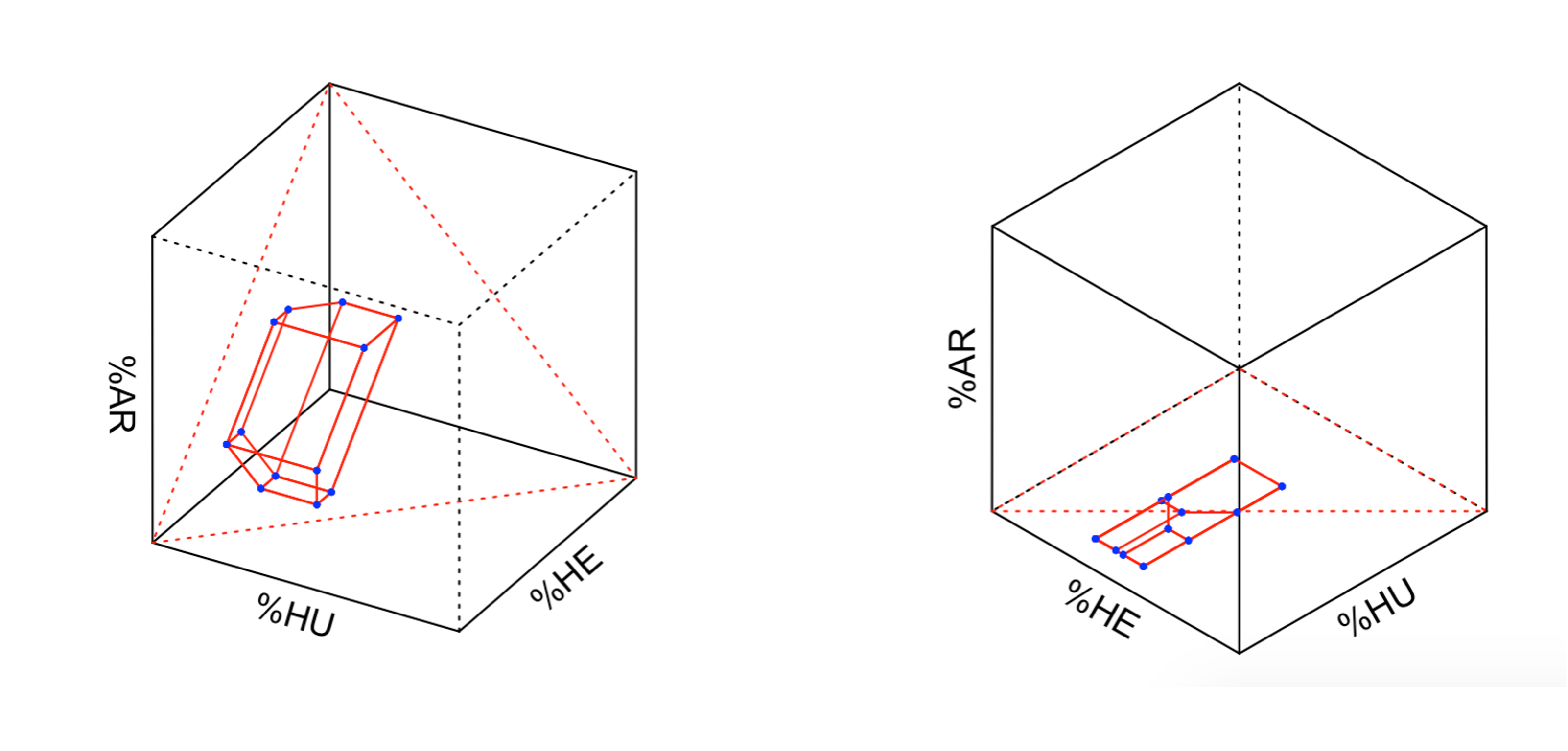
Figure 4: Variation independence of $P(Y(x_{1}))$ and $P(Y(x_{2}))$ when $K=M=2$

3 Variation (In)dependence Property on the Marginal Counterfactual Distributions $\{P(Y(x_{i})):i\in\{1,\dots,K\}\}$

[12] showed that when $X,Y$ and $Z$ are all binary, $P(Y(x_{1}))$ and $P(Y(x_{2}))$ are variation independent as shown in Figure 4. This makes it easy to compute the bounds on the $ATE=P(Y(x_{2})=2)-P(Y(x_{1})=2)$: the lower bound on ATE is the lower bound of $P(Y(x_{2})=2)$ subtracting the upper bound of $P(Y(x_{1})=2)$ while the upper bound on ATE is the upper bound of $P(Y(x_{2})=2)$ subtracting the lower bound of $P(Y(x_{1})=2)$. However, we claim that when $X$ takes more than 2 levels and $Y$ takes 2 levels, $P(Y(x_{1})),\dots,P(Y(x_{K}))$ are NOT variation independent of each other regardless of the number of levels of $Z$. This also means in the bounds relating marginals of counterfactual probabilities $\{P(Y(x_{i})):i=1,\dots,K\}$ and observed conditional probabilities $\{P(X=x,Y=y|Z=z):x=1,\dots,K,y=1,2,z=1,\dots Q\}$, there are bounds involving more than one counterfactual probability $P(Y(x_{i}))$ at a time. In this case, knowing one $P(Y(x_{i}))$ will give us additional information on the others.

3.1 binary $Z$, $X$ taking three levels, binary $Y$

Proof.

We denote $p_{xy.z}=P(X=x,Y=y\mid Z=z)$. From Theorem 1, we can write out all inequalities characterizing the joint distribution $P(Y(x_{1}),Y(x_{2}),Y(x_{3}))$.

$$P(Y(x_{3})=0)\leq p_{10.z}+p_{11.z}+p_{20.z}+p_{21.z}+p_{30.z}$$ (12)

$$P(Y(x_{3})=1)\leq p_{10.z}+p_{11.z}+p_{20.z}+p_{21.z}+p_{31.z}$$ (13)

$$P(Y(x_{2})=0)\leq p_{10.z}+p_{21.z}+p_{20.z}+p_{30.z}+p_{31.z}$$ (14)

$$P(Y(x_{2})=1)\leq p_{10.z}+p_{11.z}+p_{21.z}+p_{30.z}+p_{31.z}$$ (15)

$$P(Y(x_{1})=0)\leq p_{10.z}+p_{20.z}+p_{21.z}+p_{30.z}+p_{31.z}$$ (16)

$$P(Y(x_{1})=1)\leq p_{11.z}+p_{20.z}+p_{21.z}+p_{30.z}+p_{31.z}$$ (17)

$$P(Y(x_{2})=0,Y(x_{3})=0)\leq p_{10.z}+p_{11.z}+p_{20.z}+p_{30.z}$$ (18)

$$P(Y(x_{2})=0,Y(x_{3})=1)\leq p_{10.z}+p_{11.z}+p_{20.z}+p_{31.z}$$ (19)

$$P(Y(x_{2})=1,Y(x_{3})=0)\leq p_{10.z}+p_{11.z}+p_{21.z}+p_{30.z}$$ (20)

$$P(Y(x_{2})=1,Y(x_{3})=1)\leq p_{10.z}+p_{11.z}+p_{21.z}+p_{31.z}$$ (21)

$$P(Y(x_{1})=0,Y(x_{3})=0)\leq p_{10.z}+p_{20.z}+p_{21.z}+p_{30.z}$$ (22)

$$P(Y(x_{1})=1,Y(x_{3})=0)\leq p_{11.z}+p_{20.z}+p_{21.z}+p_{30.z}$$ (23)

$$P(Y(x_{1})=0,Y(x_{3})=1)\leq p_{10.z}+p_{20.z}+p_{21.z}+p_{31.z}$$ (24)

$$P(Y(x_{1})=1,Y(x_{3})=1)\leq p_{11.z}+p_{20.z}+p_{21.z}+p_{31.z}$$ (25)

$$P(Y(x_{1})=0,Y(x_{2})=0)\leq p_{10.z}+p_{20.z}+p_{30.z}+p_{31.z}$$ (26)

$$P(Y(x_{1})=0,Y(x_{2})=1)\leq p_{10.z}+p_{21.z}+p_{30.z}+p_{31.z}$$ (27)

$$P(Y(x_{1})=1,Y(x_{2})=0)\leq p_{11.z}+p_{20.z}+p_{30.z}+p_{31.z}$$ (28)

$$P(Y(x_{1})=1,Y(x_{2})=1)\leq p_{11.z}+p_{21.z}+p_{30.z}+p_{31.z}$$ (29)

$$P(Y(x_{1})=0,Y(x_{2})=0,Y(x_{3})=0)\leq p_{10.z}+p_{20.z}+p_{30.z}$$ (30)

$$P(Y(x_{1})=0,Y(x_{2})=1,Y(x_{3})=0)\leq p_{10.z}+p_{21.z}+p_{30.z}$$ (31)

$$P(Y(x_{1})=0,Y(x_{2})=0,Y(x_{3})=1)\leq p_{10.z}+p_{20.z}+p_{31.z}$$ (32)

$$P(Y(x_{1})=0,Y(x_{2})=1,Y(x_{3})=1)\leq p_{10.z}+p_{21.z}+p_{31.z}$$ (33)

$$P(Y(x_{1})=1,Y(x_{2})=0,Y(x_{3})=0)\leq p_{11.z}+p_{20.z}+p_{30.z}$$ (34)

$$P(Y(x_{1})=1,Y(x_{2})=1,Y(x_{3})=0)\leq p_{11.z}+p_{21.z}+p_{30.z}$$ (35)

$$P(Y(x_{1})=1,Y(x_{2})=0,Y(x_{3})=1)\leq p_{11.z}+p_{20.z}+p_{31.z}$$ (36)

$$P(Y(x_{1})=1,Y(x_{2})=1,Y(x_{3})=1)\leq p_{11.z}+p_{21.z}+p_{31.z}$$ (37)

Notice that bounds (12)-(37) can be divided to three sets:
Set 1. (12)-(17) is a bound on $P(Y(x_{i})=y_{i})$ (summation of 4 $P(Y(x_{1})=y_{1},Y(x_{2})=y_{2},Y(x_{3})=y_{3})$)
Set 2. (18)-(29) is a bound on $P(Y(x_{i})=y_{i},Y(x_{j})=y_{j})$ (summation of 2 $P(Y(x_{1})=y_{1},Y(x_{2})=y_{2},Y(x_{3})=y_{3})$)
Set 3. (30)-(37) is a bound on $P(Y(x_{1})=y_{1},Y(x_{2})=y_{2},Y(x_{3})=y_{3})$.

If we want to use bounds (12)-(37) to construct bounds on the marginal counterfactual probabilities $P(Y(x_{i})=y_{i})$, then we have the following.

1. From set 1, we will have $6\times 2=12$ bounds.
2. From set 2, we can add the inequalities pairwise - e.g. $P(Y(x_{1})=1)=P(Y(x_{1})=1,Y(x_{2})=0)+P(Y(x_{1})=1,Y(x_{2})=1)\leq p_{11.z}+p_{20.z}+p_{30.z}+p_{31.z}+p_{11.z^{\prime}}+p_{21.z}+p_{30.z^{\prime}}+p_{31.z^{\prime}}$, or $P(Y(x_{1})=1)=P(Y(x_{1})=1,Y(x_{3})=0)+P(Y(x_{1})=1,Y(x_{3})=1)\leq p_{11.z}+p_{20.z}+p_{21.z}+p_{30.z}+p_{11.z^{\prime}}+p_{20.z^{\prime}}+p_{21.z^{\prime}}+p_{31.^{\prime}}$. Notice that the right-hand side involves both levels of $Z$. Otherwise, it will be trivial since they can be implied by inequalities in set 1. Then, we can get $12*2=24$ bounds.
3. From set 3, we can first add the inequalities pairwise like in set 2 to get bounds on $P(Y(x_{i})=y_{i},Y(x_{j})=y_{j})$. Then, we have $P(Y(x_{i})=y_{i},Y(x_{j})=y_{j})=P(Y(x_{j})=y_{j})-P(Y(x_{i})=1-y_{i},Y(x_{j})=y_{j})\geq P(Y(x_{j})=y_{j})-P(Y(x_{i})=1-y_{i})$, which is an upper bound on $P(Y(x_{j})=y_{j})-P(Y(x_{i})=1-y_{i})$. In this case, we will have $12*2=24$ bounds. As seen above, these bounds involve two $P(Y(x_{i})=y_{i})$ and thus is the reason why we don’t have variation independence anymore.

Adding them together, we will have a total of 60 bounds, which is the same as what we obtain using statistical software. ∎

3.2 $Z$, $X$ taking three levels, binary $Y$

Using Theorem 1, the inequalities defining the joint counterfactual distribution $P(Y(x_{1}),Y(x_{2}),Y(x_{3}))$ are in the same form as (12)-(37) with $Z=1,2,3$. Similarly with binary $Z$, from set 1, we have $6\times 3=18$ bounds. From set 2, we have $12\times\binom{3}{2}\times 2=72$ bounds. From set 3, we also have $12\times\binom{3}{2}\times 2=72$ bounds.

With 3 levels of $Z$, after obtaining bounds on $P(Y(x_{i})=y_{i},Y(x_{j})=y_{j})$ using set 3 whose upper bounds involve two levels of $Z$-arm as described above, we could combine it with bounds in set 2 using information on the third $Z$-arm to get bounds on $P(Y(x_{i})=y_{i})$. In this way, we have $6\times 2\times 2\times\binom{3}{2}\times 2=144$ bounds.

Additionally, if we take two inequalities from set 2 (e.g. $P(Y(x_{1})=0,Y(x_{2})=0)$ and $P(Y(x_{0})=0,Y(x_{1})=0)$) and one corresponding inequality from set 3 (e.g. $P(Y(x_{0})=0,Y(x_{1})=1,Y(x_{2})=0)$ and add them together, we can get

$$P(Y(x_{2})=0,Y(x_{3})=0)+P(Y(x_{1})=0,Y(x_{2})=0)+P(Y(x_{1})=0,Y(x_{2})=1,Y(x_{3})=0)$$

$$=P(Y(x_{2})=0)-P(Y(x_{2})=0,Y(x_{3})=1)+P(Y(x_{1})=0)-P(Y(x_{1})=0,Y(x_{2})=1)$$

$$+P(Y(x_{1})=0,Y(x_{2})=1)-P(Y(x_{1})=0,Y(x_{2})=1,Y(x_{3})=1)$$

$$=P(Y(x_{2})=0)-P(Y(x_{2})=0,Y(x_{3})=1)+P(Y(x_{1})=0)$$

$$-P(Y(x_{1})=0,Y(x_{2})=1,Y(x_{3})=1)$$

$$\geq P(Y(x_{2})=0)-P(Y(x_{2})=0,Y(x_{3})=1)+P(Y(x_{1})=0)-P(Y(x_{2})=1,Y(x_{3})=1)$$

$$=P(Y(x_{2})=0)+P(Y(x_{1})=0)-P(Y(x_{3})=1),$$

which is an upper bound on $P(Y(x_{2})=0)+P(Y(x_{1})=0)-P(Y(x_{3})=1)$.

These bounds will involve all three margins of the counterfactual probabilities. There are $\binom{3}{2}\times 2\times 2\times 2\times 2\times 2\times 6=288$ bounds.

Notice that the set of bounds we obtain with binary $Z$ is always a subset of bounds we have when $Z$ takes more levels. Since $P(Y(x_{i})=y_{i})$ are not variation independent with each other with $i\in[1,3]$, they are variation dependent regardless of the number of levels in $Z$.

3.3 $X$ with more levels

We used computing software to check the variation dependence for $K=3,4,5,6$ and $Q$ up to 5 states with $M=2$.

3.4 Consequences of Variation Dependence Property

The variation dependence property is a blessing and a curse at the same time. On one hand, it makes our computation on the bounds of the ATE more complicated in that it is no longer simply a subtraction of the upper and lower bounds of each marginal counterfactual probability $P(Y(x_{i}))$. On the other hand, we might be able to get tighter bounds because of the bounds that involve multiple marginal counterfactual probabilities.

Take the situation with $K=3,M=2,Q=2$ as an example, in summary, we have bounds in the following forms

1. $P(Y(x_{i})=y)\leq 1-P(X=i,Y=1-y\mid Z=z)$

2. $P(Y(x_{i})=y)=P(Y(x_{i})=y,Y(x_{j})=0)+P(Y(x_{i})=y,Y(x_{j})=0)\leq(1-P(X=i,Y=1-y\mid Z=z)-P(X=j,Y=1\mid Z=z))+(1-P(X=j,Y=1-y\mid Z=z^{\prime})-P(X=j,Y=0\mid Z=z^{\prime}))$ where $i\neq j$

3. $P(Y(x_{i})=y)-P(Y(x_{j})=y^{\prime})\leq P(X=k,Y=0\mid Z=z)+P(X=i,Y=y\mid Z=z)+P(X=j,Y=1-y^{\prime}\mid Z=z)+P(X=k,Y=1\mid Z=z^{\prime})+P(X=i,Y=y\mid Z=z^{\prime})+P(X=j,Y=1-y^{\prime}\mid Z=z^{\prime})$ where $i\neq j\neq k$.

Denote the right-hand side of bounds in set 3 as $\tau_{ij,yy^{\prime}}$ for the simplicity of notation. Consider the treatment effect $P(Y(x_{2})=2)=P(Y(x_{1})=2)$, we can get upper and lower bounds on $P(Y(x_{1})=2)$ and $P(Y(x_{2})=2)$ separately using bounds in sets 1 and 2 above. Then, it is not hard to see if there exists a $\tau_{21,22}$ such that $\tau_{21,22}<\max_{z,z^{\prime}}P(Y(x_{2})=2)-\min_{z,z^{\prime}}P(Y(x_{1})=2)$, it will give us a tighter bound on $P(Y(x_{2})=2)=P(Y(x_{1})=2)$; see Figure 5.

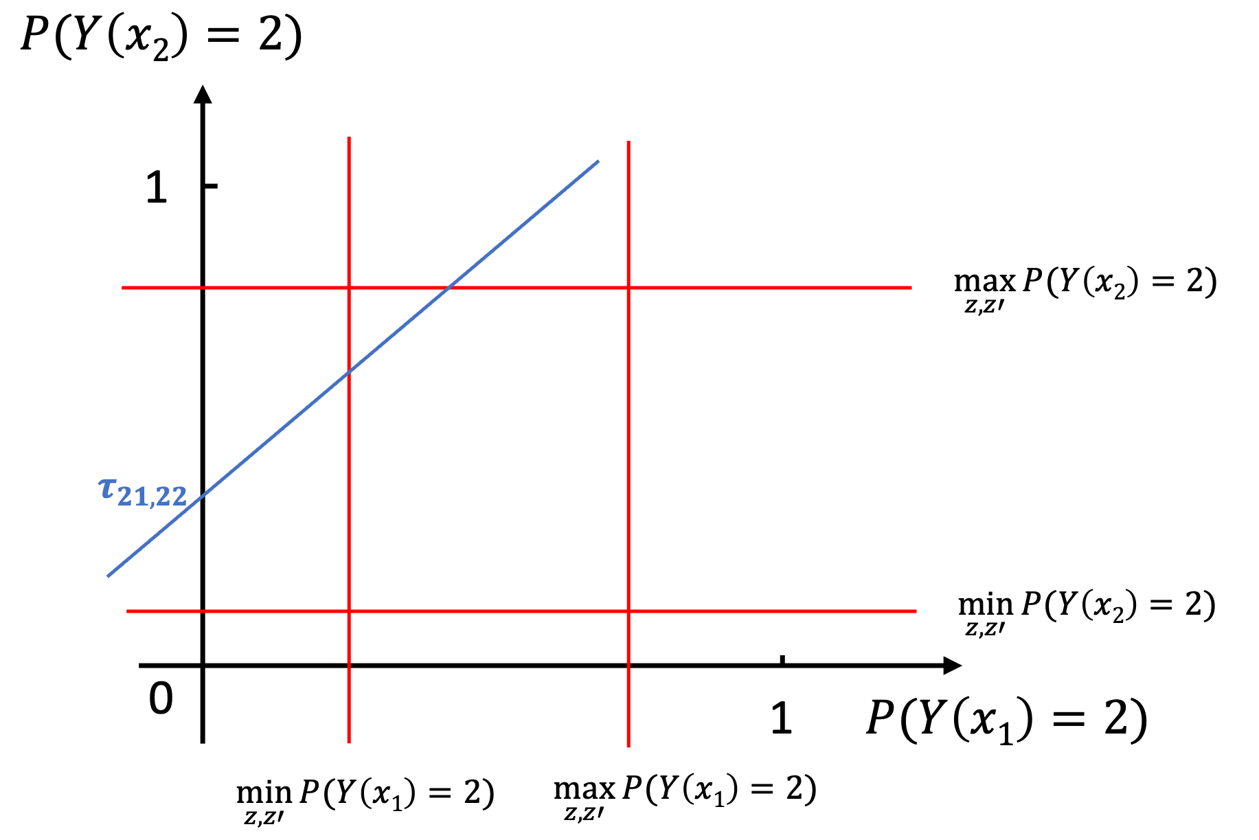
Figure 5: Example on how variation dependence property can help us with getting a tighter bound on the average causal effect.

4 Simulations on Falsification Using the Bounds and Helly’s theorem

4.1 How Likely Do We Reject the IV Model?

The proportion of the observed distribution not compatible with the IV model when $Y$ is binary is presented below. We simulated the observed probability distribution from a uniform Dirichlet distribution, $Dirich(1,\dots,1)$ with a sample size of 500. The number of Monte Carlo simulations is 200.

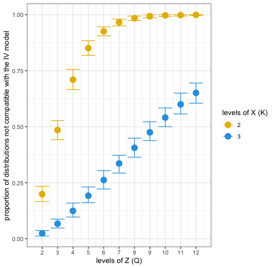
Figure 6: The proportion of empirical distributions that are not compatible with the IV model. The observed distribution is simulated under uniform Dirichlet distribution $Dirich(1,\dots,1)$. $Y$ is binary.

4.2 Reasoning Behind the Scene: Helly’s Theorem

One interesting question people might ask is if I have an instrumental variable $Z$ that takes a lot of states, i.e. $Q$ is large, do I need to check if there is any non-empty intersection of the polytope that the counterfactual distribution lives in for all possible combinations of $Z$ to make sure my observed probability distribution is compatible with the IV model? The answer is no by Helly’s Theorem. The statement of Helly’s Theorem is below.

Helly’s Theorem: Let $C_{1},...,C_{n}$ be a finite collection of convex subsets of $\mathbf{R}^{d}$, with $n\geq d+1$. If the intersection of every $d+1$ of these sets is nonempty, then the whole collection has a nonempty intersection.

In our problem, we have $d=M^{K}-1$, and this implies that when we have $Q>M^{K}$, the forms of constraints on the marginal counterfactual distributions $P(Y(x_{1})),\dots,P(Y(x_{K}))$ should be the same as $Q=M^{K}$, although the number of constraints should still be larger as $Q$ increases. Also, suppose there is a non-empty intersection of the polytope of the counterfactual distribution for any $M^{K}$ of $Z$ arms. In that case, the observed probability distribution is compatible with the IV model regardless of how large $Q$ is. When we have $K=M=2$, it is sufficient to check any 4 of $Z$ arms, and when we have $K=3$ and $M=2$, we need to check any 8 of $Z$ arms. This can be seen in Figure 6 that $Q=4$ and $Q=8$ are the turning points for the curves with $K=2$ and $K=3$ respectively.

5 Summary

In summary, we considered the instrumental variable model with categorical $Y$ taking $M$ states, categorical $X$ taking $K$ states, and categorical $Z$ taking $Q$ states, under the assumption that there is no direct effect of $Z$ on $Y$ so that $Y(x,z)=Y(x)$ and variations of independence conditions. We first provided a simple characterization of the set of joint distributions of the potential outcomes $P(Y(x_{1}),\ldots,Y(x_{K}))$ compatible with a given observed probability distribution $P(X,Y\mid Z)$. We then discussed the variation (in)dependence property on the margins $P(Y(x_{1})),\ldots,P(Y(x_{K}))$. We explored the implications for partial identification of average causal effect contrasts such as $E[Y(x_{i})-Y(x_{j})]$ and assessed the volumes of the observed distributions not compatible with the IV model. To our knowledge, our paper is the first that gives a novel closed-form characterization of the IV models with categorical treatment and outcomes and addresses other important issues as a whole.

Acknowledgments

We thank F. Richard Guo, James M. Robins and Ting Ye for helpful discussions.

References

- [1] Alexander Balke and Judea Pearl “Bounds on Treatment Effects from Studies with Imperfect Compliance” In Journal of the American Statistical Association 92.439 Taylor & Francis, 1997, pp. 1171–1176 DOI: 10.1080/01621459.1997.10474074
- [2] Arie Beresteanu, Ilya Molchanov and Francesca Molinari “Partial identification using random set theory” Annals Issue on “Identification and Decisions”, in Honor of Chuck Manski’s 60th Birthday In Journal of Econometrics 166.1, 2012, pp. 17–32 DOI: https://doi.org/10.1016/j.jeconom.2011.06.003
- [3] Blai Bonet “Instrumentality Tests Revisited” In Proceedings of the 17th Conference in Uncertainty in Artificial Intelligence, UAI ’01 San Francisco, CA, USA: Morgan Kaufmann Publishers Inc., 2001, pp. 48–55 URL: https://arxiv.org/abs/1301.2258
- [4] Stephen Burgess et al. “Guidelines for performing Mendelian randomization investigations: update for summer 2023” In Wellcome open research, 2023 URL: https://doi.org/10.12688/wellcomeopenres.15555.3
- [5] Jing Cheng and Dylan S. Small “Bounds on Causal Effects in Three-Arm Trials With Non-Compliance” In Journal of the Royal Statistical Society Series B: Statistical Methodology 68.5, 2006, pp. 815–836 DOI: 10.1111/j.1467-9868.2006.00568.x
- [6] Neil M Davies, Michael V Holmes and George Davey Smith “Reading Mendelian randomisation studies: a guide, glossary, and checklist for clinicians” In BMJ 362 BMJ Publishing Group Ltd, 2018 DOI: 10.1136/bmj.k601
- [7] Shmuel Friedland, Jingtong Ge and Lihong Zhi “Quantum Strassen’s theorem” In arXiv: Functional Analysis, 2019 URL: https://api.semanticscholar.org/CorpusID:155099804
- [8] Désiré Kédagni and Ismael Mourifié “Generalized instrumental inequalities: testing the instrumental variable independence assumption” In Biometrika 107.3, 2020, pp. 661–675 DOI: 10.1093/biomet/asaa003
- [9] Twan Koperberg “Couplings and Matchings: Combinatorial notes on Strassen’s theorem” In Statistics & Probability Letters 209, 2024, pp. 110089 DOI: https://doi.org/10.1016/j.spl.2024.110089
- [10] I Mourifié, M Henry and R Meango “Sharp bounds for the Roy model” In Unpublished manuscript, 2015
- [11] Thomas S. Richardson and James M. Robins “ACE Bounds; SEMs with Equilibrium Conditions” In Statistical Science 29.3 Institute of Mathematical Statistics, 2014, pp. 363–366 URL: http://www.jstor.org/stable/43288513
- [12] Thomas S. Richardson and James M. Robins “Assumptions and Bounds in the Instrumental Variable Model”, 2024 arXiv: https://arxiv.org/abs/2401.13758
- [13] Thomas M. Russell “Sharp Bounds on Functionals of the Joint Distribution in the Analysis of Treatment Effects” In Journal of Business & Economic Statistics 39.2 Taylor & Francis, 2021, pp. 532–546 DOI: 10.1080/07350015.2019.1684300
- [14] Eleanor Sanderson et al. “Mendelian randomization” In Nature Reviews Methods Primers, 2022 URL: https://doi.org/10.1038/s43586-021-00092-5
- [15] V. Strassen “The Existence of Probability Measures with Given Marginals” In The Annals of Mathematical Statistics 36.2 Institute of Mathematical Statistics, 1965, pp. 423–439 DOI: 10.1214/aoms/1177700153
- [16] Sonja A. Swanson, Matthew Miller Miguel A., James M. Robins and Thomas S. Richardson “Partial Identification of the Average Treatment Effect Using Instrumental Variables: Review of Methods for Binary Instruments, Treatments, and Outcomes” PMID: 31537952 In Journal of the American Statistical Association 113.522 Taylor & Francis, 2018, pp. 933–947 DOI: 10.1080/01621459.2018.1434530
- [17] Sonja A. Swanson, James M. Robins, Matthew Miller and Miguel A. Hernán “Selecting on Treatment: A Pervasive Form of Bias in Instrumental Variable Analyses” In American Journal of Epidemiology 181.3, 2015, pp. 191–197 DOI: 10.1093/aje/kwu284