Double Robustness of Local Projections
and Some Unpleasant VARithmetic

Abstract:

We consider impulse response inference in a locally misspecified stationary vector autoregression (VAR) model. The conventional local projection (LP) confidence interval has correct coverage even when the misspecification is so large that it can be detected with probability approaching 1. This follows from a “double robustness” property analogous to that of modern estimators for partially linear regressions. In contrast, VAR confidence intervals dramatically undercover even for misspecification so small that it is difficult to detect statistically and cannot be ruled out based on economic theory. This is because of a “no free lunch” result for VARs: the worst-case bias and coverage distortion are small if, and only if, the variance is close to that of LP. While VAR coverage can be restored by using a bias-aware critical value or a large lag length, the resulting confidence interval tends to be at least as wide as the LP interval.

Keywords: bias-aware inference, double robustness, local projection, misspecification, structural vector autoregression. JEL codes: C22, C32.

1 Introduction

In recent years, local projection (LP) estimators of impulse response functions have become a very popular alternative to structural vector autoregressions (henceforth interchangeably referred to as VAR or SVAR, Sims, 1980). In addition to their simplicity, one potential explanation for the popularity of LPs is their perceived robustness to misspecification, as claimed by Jordà (2005) in his seminal article that proposed the estimation method:

“[T]hese projections are local to each forecast horizon and therefore more robust [than VARs] to misspecification of the unknown DGP.”

While this sentiment has been echoed in influential reviews (e.g., see Ramey, 2016; Nakamura and Steinsson, 2018; Jordà, 2023), there so far exist essentially no theoretical results on the relative robustness of LP and VAR inference procedures to misspecification. Plagborg-Møller and Wolf (2021) and Xu (2023) show that the two estimators are in fact asymptotically equivalent—and thus equally robust to misspecification—in a general VAR($\infty$) model if the estimation lag length diverges to infinity with the sample size. However, this result does not directly speak to the empirically relevant case where researchers employ small-to-moderate lag lengths to preserve degrees of freedom. Applied researchers must therefore base their choice of inference procedure on empirically calibrated simulation studies (Kilian and Kim, 2011; Li, Plagborg-Møller, and Wolf, 2024).

The main contribution of this paper is to provide a formal proof of the claim in Jordà (2005) that conventional LP confidence intervals for impulse responses are surprisingly robust to misspecification. At the same time, we show that VAR confidence intervals are unreliable in the face of even small amounts of misspecification.

To formalize our results, we consider a large class of stationary data generating processes (DGPs) that are well approximated by a finite-order SVAR model, but subject to local misspecification in the form of an asymptotically vanishing moving average (MA) process, of potentially infinite order. This class of models covers many types of dynamic misspecification, such as under-specification of the lag length, failure to include relevant control variables, inappropriate aggregation, measurement error, and omitted nonlinearities. In particular, such an environment is consistent with essentially all linearized structural macroeconomic models (Fernández-Villaverde, Rubio-Ramírez, Sargent, and Watson, 2007). Intuitively, our set-up with local misspecification captures the idea that finite-order VAR models provide a good—but not perfect—approximation of reality.

In this setting, we prove that the conventional LP confidence interval has correct (pointwise) asymptotic coverage even for local misspecification that is of such a large magnitude that it can be detected with probability 1 in large samples. This robustness property requires that we control for those lags of the data that are strong predictors of the outcome or impulse variables, but crucially for applied work, the omission of lags with small-to-moderate predictive power does not threaten coverage. We argue that our result can be interpreted as a consequence of the double robustness of the LP estimator, which is analogous to the double robustness of modern partially linear regression estimators in the literature on debiased machine learning (Newey, 1990; Chernozhukov, Chetverikov, Demirer, Duflo, Hansen, Newey, and Robins, 2018; Chernozhukov, Escanciano, Ichimura, Newey, and Robins, 2022).

In stark contrast to LP, small amounts of misspecification cause conventional VAR confidence intervals for impulse responses to suffer from severe under-coverage asymptotically. We derive analytically the worst-case bias and coverage of VARs over all possible misspecification processes, subject to a constraint only on the overall magnitude of the misspecification. A “no free lunch” result for VARs emerges: the worst-case bias and coverage distortion are small if, and only if, the asymptotic variance is close to that of LP. This worst-case result is practically relevant—VAR confidence intervals severely undercover even when the misspecification term: (i) is small in magnitude; (ii) has dynamic properties that cannot be ruled out ex ante based on economic theory; and (iii) is difficult to detect ex post with model specification tests. While the coverage can be restored by using a larger bias-aware critical value (Armstrong and Kolesár, 2021) or by using a large number of lags for estimation, the resulting confidence intervals are so wide that one may as well report the LP interval.

We demonstrate through simulations that our asymptotic results are useful to understand the finite-sample trade-off between LP and VAR confidence intervals. We first consider a univariate ARMA(1,1) model. While LP confidence intervals here have coverage close to the nominal level, confidence intervals based on short-lag autoregressions severely undercover when the MA coefficient is only moderately large. In fact, in this simple case the implied MA misspecification is very close to the theoretical worst case. We next run simulations based on the medium-scale structural macroeconomic model of Smets and Wouters (2007). The researcher estimates the impulse response function of inflation with respect to an observed cost-push shock, with lag length selected by the Akaike Information Criterion (AIC). VAR confidence intervals materially undercover—particularly at medium and long horizons—while LP again attains close to nominal coverage. Consistent with our theoretical results, increasing the estimation lag length ameliorates the VAR coverage, but at the cost of delivering confidence intervals as wide as those of LP.

Other literature.

Relative to the previously cited simulation studies of LPs and VARs, we derive analytical results on the worst-case asymptotic properties of these inference procedures that hold for a wide range of stationary, locally misspecified VAR models. The empirically calibrated simulations in Li, Plagborg-Møller, and Wolf (2024) suggest a stark bias-variance trade-off between LP (low bias, high variance) and VAR estimators (moderate bias, low variance). The reason behind the theoretical superiority of LP proved in this paper is that, if the objective is to construct confidence intervals, then even a moderate amount of VAR bias cannot be tolerated, as it causes the VAR confidence interval to be poorly centered. Effectively, a concern for confidence interval coverage induces a large weight on bias in the researcher’s objective function, justifying the use of LP despite its higher variance.

The robustness of LP to misspecification discussed here—with stationary data and at fixed horizons—is conceptually and theoretically distinct from the robustness of LP to the persistence in the data and the length of the impulse response horizon shown by Montiel Olea and Plagborg-Møller (2021). Nevertheless, it turns out that controlling for lags (“lag augmentation”) is key to all the robustness properties established in Montiel Olea and Plagborg-Møller (2021) and the present paper.

We also build upon previous research into misspecified VAR models, uncovering novel results about the robustness of LPs and the worst-case properties of VAR procedures. Braun and Mittnik (1993) derive expressions for the probability limits of VAR estimators under global MA misspecification, but do not provide analytical results on the performance of inference procedures. Schorfheide (2005) characterizes the asymptotic mean squared errors of iterated and direct multi-step forecasts in a reduced-form VAR model with MA terms of order $T^{-1/2}$. Müller and Stock (2011) construct Bayesian forecast intervals in a locally misspecified univariate AR model. Relative to these papers, we contribute by: (i) focusing on structural impulse responses rather than forecasting; (ii) allowing for more general rates of local misspecification, key to uncovering the double robustness of LP; and (iii) deriving simple analytical formulas for the worst-case bias and coverage of VARs. As such, our results formalize concerns by some applied practitioners about the lack of VAR robustness (e.g., Chari, Kehoe, and McGrattan, 2008; Nakamura and Steinsson, 2018).

Whereas our paper deals with bias imparted by dynamic misspecification, our asymptotics abstract from the order-$T^{-1}$ bias of LPs and VARs that is due to persistence in the data (Pope, 1990; Kilian, 1998; Herbst and Johannsen, 2023).

Outline.

Section 2 provides an overview of our main results in a univariate model. Section 3 introduces the general local-to-SVAR($p$) model, defines LP and VAR estimators, and proves the robustness of LP and fragility of VAR confidence intervals. Section 4 derives analytically the worst-case bias and coverage of VARs, and shows that bias-aware VAR confidence intervals tend to be wider than the LP interval. Section 5 demonstrates the practical relevance of our results through simulations. Section 6 concludes. Proofs and supplementary results are relegated to the appendix and an online supplement.

Notation.

All asymptotic limits are taken as the sample size $T\to\infty$ and are pointwise in the sense of fixing the true model parameters and the impulse response horizon. A sum $\sum_{\ell=a}^{b}c_{\ell}$ is defined to equal 0 when $a>b$.

2 Overview of results

In this section we illustrate our main results in a simple special case, namely a univariate autoregressive (AR) model subject to misspecification in the form of a small moving average (MA) process. In the subsequent sections we will show that all qualitative results—as well as many quantitative ones—from the simple model carry over to a general class of multivariate SVAR models with local MA misspecification.

Model and assumptions.

Suppose the data $\{y_{t}\}_{t=1}^{T}$ satisfies a univariate, stationary local-to-AR(1) model

$$y_{t}=\rho y_{t-1}+[1+T^{-\zeta}\alpha(L)]\varepsilon_{t}\quad\text{for all }t,$$ (2.1)

where $\alpha(L)=\sum_{\ell=1}^{\infty}\alpha_{\ell}L^{\ell}$ is a potentially infinite-order lag polynomial. This model captures the idea that the time series dynamics of the data are well approximated by a simple autoregressive model (here an AR(1)) driven by an unobserved white noise shock $\varepsilon_{t}$, but with a small amount of misspecification in the form of an MA process $T^{-\zeta}\alpha(L)\varepsilon_{t}$. The misspecification is asymptotically small in the sense that the MA coefficients converge to zero at the rate $T^{-\zeta}$, though the misspecification may still affect the properties of estimators, as shown by Schorfheide (2005) and as demonstrated below. We argue below in Section 3.1 that MA misspecification of this form can capture many empirically relevant types of dynamic misspecification, such as under-specification of the lag length, missing control variables, inappropriate aggregation, and measurement error. We consider local rather than global misspecification in the spirit of local power analysis (e.g., Rothenberg, 1984), since this makes the bias-variance trade-off between the AR and LP estimators matter even asymptotically as the sample size diverges, allowing us to make tractable analytical comparisons between these two procedures.

Assumption 2.1.

For each $T$, $\{y_{t}\}_{t\in\mathbb{Z}}$ is the stationary solution to the equation (2.1), where the shocks and parameters satisfy the following conditions:

1. $\varepsilon_{t}\overset{i.i.d.}{\sim}(0,\sigma^{2})$ with $\sigma^{2}>0$ and $E(\varepsilon_{t}^{4})<\infty$.

2. $\rho\in(-1,1)$.

3. $\alpha(L)$ is absolutely summable.

4. $\zeta>1/4$.

Absolute summability of $\alpha(L)$ is a weak regularity condition ensuring the MA($\infty$) process $\alpha(L)\varepsilon_{t}$ is well-defined (Brockwell and Davis, 1991, Proposition 3.1.1). The significance of the assumption that misspecification vanishes faster than $T^{-1/4}$ will become clear below.

The parameter of interest is the impulse response of $y_{t+h}$ with respect to $\varepsilon_{t}$ according to the model (2.1):

$$\theta_{h,T}\equiv E[y_{t+h}\mid\varepsilon_{t}=1]-E[y_{t+h}\mid\varepsilon_{t}=0]=\rho^{h}+T^{-\zeta}\sum_{\ell=1}^{h}\rho^{h-\ell}\alpha_{\ell},\quad h=0,1,2,\dots.$$

The first term is the usual AR(1) formula, while the second term arises from the MA component. Importantly, and consistent with our focus on the consequences of dynamic misspecification, we do not treat the VAR misspecification as non-classical measurement error that should be ignored for structural analysis; instead, the true causal model has an ARMA form (with small but potentially non-zero MA terms), and we care about the full transmission mechanism of shocks in this model.

Estimators.

We will consider two estimators of the impulse response of interest $\theta_{h,T}$ using the data $\{y_{t}\}_{t=1}^{T}$:

1. The LP estimator $\hat{\beta}_{h}$ is obtained from an OLS regression

   $$y_{t+h}=\hat{\beta}_{h}y_{t}+\hat{\gamma}_{h}y_{t-1}+\hat{\xi}_{h,t},$$ (2.2)

   where we control for one lag of the data, and $\hat{\xi}_{h,t}$ is the OLS residual.

2. The AR estimator $\hat{\delta}_{h}$ is given by

   $$\hat{\delta}_{h}=\hat{\rho}^{h},\quad\text{where}\quad\hat{\rho}=\frac{\sum_{t=2}^{T}y_{t}y_{t-1}}{\sum_{t=2}^{T}y_{t-1}^{2}}.$$

The two estimators coincide at the impact horizon, $\hat{\beta}_{0}=\hat{\delta}_{0}$. Conventional confidence intervals based on both these estimators would have correct asymptotic coverage in a well-specified AR(1) model. However, the presence of the MA term in the model (2.1) means that, in principle, both the LP and VAR estimators ought to control for infinitely many lags of the data rather than just one. Nevertheless, we shall now see that this dynamic misspecification has much more serious consequences for the AR procedure than for LP.

Robustness of LP.

Our first main result is that the limiting distribution of the LP estimator is remarkably robust to the presence of local misspecification.

Proposition 2.1.

Under Assumption 2.1,

$$\hat{\beta}_{h}-\theta_{h,T}=\frac{1}{\sigma^{2}}\frac{1}{T}\sum_{t=1}^{T}\xi_{h,t}\varepsilon_{t}+o_{p}(T^{-1/2}),$$

where $\xi_{h,t}\equiv\sum_{\ell=1}^{h}\rho^{h-\ell}\varepsilon_{t+\ell}$ is the $h$-step-ahead forecast error.

Since the above asymptotic representation is invariant to the MA misspecification, the limiting distribution of LP is the same as it would be in a correctly specified AR(1) model (provided $\zeta>1/4$, as imposed in Assumption 2.1). Though this robustness of LP is with respect to local (i.e., asymptotically vanishing) misspecification, it is still quantitatively meaningful, as MA terms of order $T^{-\zeta}$ with $\zeta\in(1/4,1/2)$ can be detected with probability 1 asymptotically by conventional AR model specification tests, such as the Hausman test considered in Section 3.3 below.

Why is LP robust to misspecification of such large magnitude? We will offer two mathematically equivalent pieces of intuition, with our discussion here deliberately heuristic. First, the classic omitted variable bias formula suggests that the bias of the LP impulse response estimator $\hat{\beta}_{h}$ in the regression (2.2) is proportional to the product of two factors: (i) the direct effect of omitted lags on $y_{t+h}$, and (ii) the covariance of the residualized regressor of interest $y_{t}-E[y_{t}\mid y_{t-1}]=\varepsilon_{t}+O_{p}(T^{-\zeta})$ with the omitted lags. The factor (i) is of order $T^{-\zeta}$ in the local-to-AR(1) model (2.1). The factor (ii) is also of order $T^{-\zeta}$, since $\varepsilon_{t}$ is uncorrelated with any lagged data. Hence, the OVB is of order $T^{-2\zeta}=o(T^{-1/2})$ under the assumption $\zeta>1/4$, and thus the bias of the estimator is negligible relative to the standard deviation, which is of order $T^{-1/2}$ as in the correctly specified case.

The preceding intuition is a special case of the double robustness property of partially linear regressions (see Example 1 in Chernozhukov, Escanciano, Ichimura, Newey, and Robins, 2022), which we will now argue applies also to LP, again settling for a heuristic argument. Consider any dynamic model (for example a VARMA($p,q$)) that implies the following local projection representation:

$$y_{t+h}=\theta_{0,h}y_{t}+\gamma_{0}(y^{t-1})+\xi_{h,t},\quad\text{where}\quad\xi_{h,t}\mathchoice{\mathrel{\hbox to0.0pt{$\displaystyle\perp$\hss}\mkern 2.0mu{\displaystyle\perp}}}{\mathrel{\hbox to0.0pt{$\textstyle\perp$\hss}\mkern 2.0mu{\textstyle\perp}}}{\mathrel{\hbox to0.0pt{$\scriptstyle\perp$\hss}\mkern 2.0mu{\scriptstyle\perp}}}{\mathrel{\hbox to0.0pt{$\scriptscriptstyle\perp$\hss}\mkern 2.0mu{\scriptscriptstyle\perp}}}y^{t}\equiv(y_{t},y_{t-1},\dots).$$

Here $\theta_{0,h}$ is the true impulse response, and $\gamma_{0}(\cdot)$ is a function of lagged data. Define $\nu_{0}(y^{t-1})\equiv E[y_{t}\mid y^{t-1}]$. By applying the Frisch-Waugh lemma to the regression (2.2), the LP estimator $\hat{\beta}_{h}$ is the sample analogue of the solution $\theta_{0,h}$ to the moment condition

$$E[\{y_{t+h}-\theta_{0,h}y_{t}-\gamma_{0}(y^{t-1})\}\{y_{t}-\nu_{0}(y^{t-1})\}]=0.$$

If we evaluate the moment on the left-hand side at arbitrary functions $\gamma(\cdot)$ and $\nu(\cdot)$ rather than at the true ones $\gamma_{0}(\cdot)$ and $\nu_{0}(\cdot)$, a simple calculation shows that it equals $E[\{\gamma_{0}(y^{t-1})-\gamma(y^{t-1})\}\{\nu_{0}(y^{t-1})-\nu(y^{t-1})\}]$. Hence, the moment condition is satisfied at the true impulse response parameter $\theta_{0,h}$ as long as either $\gamma=\gamma_{0}$ or $\nu=\nu_{0}$, making the LP estimator doubly robust: it is consistent if we correctly specify either the controls $\gamma(y^{t-1})$ in the outcome equation or the controls $\nu(y^{t-1})$ in the implicit first-stage regression that isolates the shock $\varepsilon_{t}=y_{t}-\nu(y^{t-1})$. Whereas in the present univariate model the choices of $\gamma(\cdot)$ and $\nu(\cdot)$ are necessarily linked, in the general multivariate model in Section 3 they are decoupled, and as a result it is possible to correctly specify the controls in the outcome equation while mis-identifying the shock, and vice versa. As a consequence of double robustness, and as argued more generally by Chernozhukov, Chetverikov, Demirer, Duflo, Hansen, Newey, and Robins (2018) (and confirmed by our proof), it turns out that estimation error in $\gamma_{0}$ and $\nu_{0}$ only affects the asymptotic distribution of the doubly robust estimator $\hat{\beta}_{h}$ through the product of the estimation errors $\|\hat{\gamma}-\gamma_{0}\|\times\|\hat{\nu}-\nu_{0}\|$. In our local-to-AR(1) model (2.1), both terms in this product are of order $T^{-\zeta}$ due to the omitted lags. The product is then of order $T^{-2\zeta}=o(T^{-1/2})$ and thus asymptotically negligible, consistent with our earlier intuition.

Fragility of AR.

Our second main result is that this (double) robustness of LP to misspecification stands in stark contrast to the fragility of the AR estimator.

Proposition 2.2.

Under Assumption 2.1,

$$\hat{\delta}_{h}-\theta_{h,T}=T^{-\zeta}\operatorname{aBias}(\hat{\delta}_{h})+\frac{h\rho^{h-1}(1-\rho^{2})}{\sigma^{2}}\frac{1}{T}\sum_{t=1}^{T}\varepsilon_{t}\tilde{y}_{t-1}+o_{p}(T^{-\zeta}+T^{-1/2}),$$ (2.3)

where $\tilde{y}_{t}=(1-\rho L)^{-1}\varepsilon_{t}$ satisfies a correctly specified AR(1) model with $\alpha(L)=0$, and the asymptotic bias is

$$\operatorname{aBias}(\hat{\delta}_{h})\equiv\underbrace{h\rho^{h-1}}_{\frac{\partial(\rho^{h})}{\partial\rho}}\underbrace{(1-\rho^{2})\sum_{\ell=1}^{\infty}\rho^{\ell-1}\alpha_{\ell}}_{\operatorname{aBias}(\hat{\rho})=\frac{\operatorname*{Cov}(\alpha(L)\varepsilon_{t},\tilde{y}_{t-1})}{\operatorname*{Var}(\tilde{y}_{t-1})}}-\underbrace{\sum_{\ell=1}^{h}\rho^{h-\ell}\alpha_{\ell}}_{\theta_{h,T}-\rho^{h}}.$$ (2.4)

The convergence rate of the AR estimator is $T^{-\min\{1/2,\zeta\}}$, potentially slower than the $T^{-1/2}$ rate achieved by LP. This is because the AR estimator suffers from an asymptotic bias of order $T^{-\zeta}$. This bias is due to two forces: first, the AR(1) coefficient $\hat{\rho}$ is biased due to the endogeneity caused by the MA terms, and second, the AR estimator extrapolates the horizon-$h$ impulse response based on a parametric formula $\hat{\rho}^{h}$ that does not hold exactly in the true model (2.1). The second term on the right-hand side of the asymptotic representation (2.3) is the same as it would be in the correctly specified AR(1) model (with $\alpha(L)=0$), and therefore of order $T^{-1/2}$. As a consequence, the AR bias is only asymptotically negligible if $\zeta>1/2$, a much smaller degree of robustness than shown above for LP. The case $\zeta=1/2$ is of particular interest, as then the bias and standard deviation are of the same asymptotic order (see also Schorfheide, 2005). MA terms of order $T^{-1/2}$ can be detected with asymptotic probability strictly between 0 and 1 by specification tests, as will be shown below in Section 3.3.

Implications for inference.

Consider the conventional level-$(1-a)$ confidence intervals based on the LP and AR estimators, respectively:

$$\operatorname{CI}(\hat{\beta}_{h})\equiv\left[\hat{\beta}_{h}\pm z_{1-a/2}\sqrt{\operatorname{aVar}(\hat{\beta}_{h})/T}\right],\quad\operatorname{CI}(\hat{\delta}_{h})\equiv\left[\hat{\delta}_{h}\pm z_{1-a/2}\sqrt{\operatorname{aVar}(\hat{\delta}_{h})/T}\right],$$ (2.5)

where $z_{1-a/2}\equiv\Phi^{-1}(1-a/2)$ is the normal critical value, $\Phi(\cdot)$ is the standard normal cumulative distribution function, and the asymptotic variances $\operatorname{aVar}(\hat{\beta}_{h})$ and $\operatorname{aVar}(\hat{\delta}_{h})$ correspond to the variances of the leading stochastic terms in Propositions 2.1 and 2.2, yielding the same expressions as in the correctly specified case. While we use the asymptotic variances in the definition of the confidence intervals for mathematical simplicity, the results would be the same if we used the conventional (estimated) standard error formulas that apply under correct specification, since the latter are consistent under Assumption 2.1.

Corollary 2.1.

Under Assumption 2.1, $\lim_{T\to\infty}P(\theta_{h,T}\in\operatorname{CI}(\hat{\beta}_{h}))=1-a$. If moreover $\operatorname{aVar}(\hat{\delta}_{h})>0$ and $\operatorname{aBias}(\hat{\delta}_{h})\neq 0$, then $\lim_{T\to\infty}P(\theta_{h,T}\in\operatorname{CI}(\hat{\delta}_{h}))=0$ for $\zeta\in(1/4,1/2)$, and $\lim_{T\to\infty}P(\theta_{h,T}\in\operatorname{CI}(\hat{\delta}_{h}))<1-a$ for $\zeta=1/2$.

The corollary shows that the LP confidence interval robustly controls coverage. In contrast, except in the knife-edge case where the asymptotic bias equals 0, the AR confidence interval has coverage converging to 0 for misspecification of order $T^{-\zeta}$ with $\zeta\in(1/4,1/2)$, while the asymptotic coverage is strictly below the nominal level $1-a$ for $\zeta=1/2$. This is because the AR interval has the same width as in the correctly specified model, but it is incorrectly centered due to the bias.

Worst-case bias and coverage.

While we have shown that the AR confidence interval can severely under-cover asymptotically, it is natural to ask whether such poor performance is likely in practice. To answer this question, we set $\zeta=1/2$, ensuring that the bias-variance trade-off is non-trivial; otherwise the bias either dominates or is negligible asymptotically. Next, we restrict the misspecification to be small, in the sense that the noise-to-signal ratio $\operatorname*{Var}(T^{-1/2}\alpha(L)\varepsilon_{t})/\operatorname*{Var}(\varepsilon_{t})$ in the local-to-AR(1) model (2.1) is bounded by $M^{2}/T$ for a given $M$. Under this constraint, the worst-case VAR bias is strikingly simple.

Proposition 2.3.

Under Assumption 2.1, $\zeta=1/2$, and $\operatorname{aVar}(\hat{\delta}_{h})>0$,

$$\max_{\alpha(L)\colon\operatorname*{Var}(\alpha(L)\varepsilon_{t})/\sigma^{2}\leq M^{2}}\frac{|\operatorname{aBias}(\hat{\delta}_{h})|}{\sqrt{\operatorname{aVar}(\hat{\delta}_{h})}}=M\sqrt{\frac{\operatorname{aVar}(\hat{\beta}_{h})}{\operatorname{aVar}(\hat{\delta}_{h})}-1}.$$ (2.6)

This formula implies that there is no free lunch for the AR estimator: whenever the relative standard error $\sqrt{\operatorname{aVar}(\hat{\delta}_{h})/\operatorname{aVar}(\hat{\beta}_{h})}$ of the AR and LP estimators is small, the AR estimator is vulnerable to misspecification in the sense of a large worst-case bias, unless we are certain a priori that the noise-to-signal ratio $M^{2}/T$ is extremely small. It turns out that the exact same worst-case bias formula applies to multivariate locally misspecified VAR models with multiple lags, as shown below in Section 4.1. Hence, while it is possible to ameliorate the worst-case bias of AR estimators by increasing the lag length, this can only happen at the expense of increasing the variance.

As an implication of the above result, we show analytically in Section 4 that the AR confidence interval has severely distorted worst-case coverage when the relative standard error of AR relative to LP lies in an empirically relevant range. These severe distortions are achieved by MA misspecification processes that (i) are small, (ii) cannot be ruled out ex ante using economic theory, and (iii) are difficult to detect ex post using model specification tests. While it is possible to construct a valid bias-aware AR confidence interval with a larger critical value that takes into account the worst-case bias (following the general recipe of Armstrong and Kolesár, 2021), this interval tends to be wider than the equally valid conventional LP confidence interval unless the noise-to-signal ratio is restricted to be extremely small. We conclude that AR inference is only reliable when using a lag length that is so large that the procedure becomes equivalent with LP.

3 Robust local projections, fragile VARs

We now state our general model and assumptions, define the general LP and VAR impulse response estimators, derive the asymptotic representations of these estimators, and draw conclusions about their relative robustness to misspecification. While LP is shown to be robust to large amounts of misspecification, the VAR estimator is fragile in that it suffers from generically non-negligible asymptotic bias.

3.1 Model and assumptions

We consider a multivariate, stationary structural VARMA($1,\infty$) model that is local to an SVAR(1) model:

$$y_{t}=Ay_{t-1}+H[I+T^{-\zeta}\alpha(L)]\varepsilon_{t}\quad\text{for all }t,$$ (3.1)

where $y_{t}=(y_{1,t},\dots,y_{n,t})^{\prime}$ is $n$-dimensional, $\varepsilon_{t}=(\varepsilon_{1,t},\dots,\varepsilon_{m,t})^{\prime}$ is $m$-dimensional, $A$ is an $n\times n$ matrix, $H$ is an $n\times m$ matrix, and $\alpha(L)=\sum_{\ell=1}^{\infty}\alpha_{\ell}L^{\ell}$ is an $m\times m$ lag polynomial. We allow the number of shocks $m$ to potentially exceed the number of variables $n$, and vice versa. We will show below that equation (3.1) encompasses local-to-SVAR models with $p>1$ lags by writing them in companion form.

The parameter of interest is the response at horizon $h$ of the variable $y_{i^{*},t}$ with respect to the shock $\varepsilon_{j^{*},t}$ for some indices $i^{*}\in\{1,\dots,n\}$ and $j^{*}\in\{1,\dots,m\}$. We define this parameter formally below.

Assumption 3.1.

For each $T$, $\{y_{t}\}_{t\in\mathbb{Z}}$ is the stationary solution to equation (3.1), given the following restrictions on parameters and shocks:

1. $\varepsilon_{t}\overset{i.i.d.}{\sim}(0_{m\times 1},D)$, where $D\equiv\operatorname*{diag}(\sigma_{1}^{2},\dots,\sigma_{m}^{2})$. For all $j=1,\dots,m$, $\sigma_{j}^{2}>0$ and $E(\varepsilon_{j,t}^{4})<\infty$.

2. All eigenvalues of $A$ are strictly below 1 in absolute value.

3. The first $j^{*}$ rows of $H$ are of the form $(\tilde{H},0_{j^{*}\times(m-j^{*})})$, where $\tilde{H}$ is a $j^{*}\times j^{*}$ lower triangular matrix with 1’s on the diagonal. In particular, we require $j^{*}\leq n$.

4. $S\equiv\operatorname*{Var}(\tilde{y}_{t})$ is non-singular, where $\tilde{y}_{t}\equiv(I-AL)^{-1}H\varepsilon_{t}$ is the stationary solution to (3.1) when $\alpha(L)=0$. Specifically, $\operatorname*{vec}(S)=(I-A\otimes A)^{-1}\operatorname*{vec}(\Sigma)$, where $\Sigma\equiv HDH^{\prime}$.

5. $\alpha(L)$ is absolutely summable.

6. $\zeta>1/4$.

The assumption of shock homoskedasticity is made for analytical convenience, though we expect that our qualitative conclusions about the robustness of LP and the asymptotic bias of VAR will go through under various forms of conditional heteroskedasticity. The assumptions on $H$ correspond to recursive (also known as Cholesky) identification of the shock of interest $\varepsilon_{j^{*},t}$, with a unit effect normalization $H_{j^{*},j^{*}}=1$. A special case is when the shock is directly observed, which corresponds to ordering it first (i.e., $j^{*}=1$). It is a minor extension to allow for identification via external instruments (also known as proxies), as this just requires ordering the instrument $y_{1,t}$ first and adding an additional measurement error term to the first equation (Stock and Watson, 2018; Plagborg-Møller and Wolf, 2021).

The impulse response of interest is now defined as

$$\theta_{h,T}\equiv E[y_{i^{*},t+h}\mid\varepsilon_{j^{*},t}=1]-E[y_{i^{*},t+h}\mid\varepsilon_{j^{*},t}=0]=e_{i^{*},n}^{\prime}\left(A^{h}H+T^{-\zeta}\sum_{\ell=1}^{h}A^{h-\ell}H\alpha_{\ell}\right)e_{j^{*},m},$$

where $e_{i,n}$ denotes the $n$-dimensional unit vector with a 1 in position $i$.

Additional lags.

Our framework covers local-to-SVAR($p$) models of the form

$$\check{y}_{t}=\sum_{\ell=1}^{p}\check{A}_{\ell}\check{y}_{t-\ell}+\check{H}[I+T^{-\zeta}\alpha(L)]\varepsilon_{t},$$ (3.2)

where $\check{y}_{t}$ is $\check{n}$-dimensional, the $\check{A}_{\ell}$ matrices are $\check{n}\times\check{n}$, and $\check{H}$ is $\check{n}\times m$ and satisfies Assumption 3.1(iii). This fits into the original model (3.1) if we set $n=\check{n}p$ and define the companion form representation

$$y_{t}=\begin{pmatrix}\check{y}_{t}\\ \check{y}_{t-1}\\ \check{y}_{t-2}\\ \vdots\\ \check{y}_{t-p+1}\end{pmatrix},\quad A=\begin{pmatrix}\check{A}_{1}&\check{A}_{2}&\dots&\check{A}_{p-1}&\check{A}_{p}\\ I&0&\dots&0&0\\ 0&I&\dots&0&0\\ \vdots&&\ddots&&\vdots\\ 0&0&\dots&I&0\end{pmatrix},\quad H=\begin{pmatrix}\check{H}\\ 0\\ 0\\ \vdots\\ 0\end{pmatrix}.$$

In particular, we can allow the estimation lag length $p$ to exceed the true minimal lag length $p_{0}$ of the model by setting $\check{A}_{\ell}=0$ for $\ell>p_{0}$. This extension will prove useful when we consider what happens as the lag length of the estimated VAR is increased.

Types of misspecification.

The local-to-SVAR model (3.1) with MA misspecification covers several empirically relevant types of misspecification. While essentially all modern discrete-time, linearized DSGE macro models have VARMA representations, they usually cannot be represented exactly as finite-order VAR models (e.g., Giacomini, 2013). Even if the true DGP were a finite-order VAR, dynamic misspecification of the estimation model can give rise to MA terms, for example due to under-specification of the lag length or failing to control for some of the variables in the true VAR system. Relatedly, MA terms may arise from a failure of invertibility of the shocks (Alessi, Barigozzi, and Capasso, 2011). VARMA representations can also arise from temporal or cross-sectional aggregation of finite-order VAR models, including contamination by classical measurement error (e.g., Granger and Morris, 1976; Lütkepohl, 1984). In all of these cases, if the number of lags used for estimating the VAR is chosen to be sufficiently large, then the MA remainder will be small in magnitude, which is consistent with the spirit of our locally misspecified model (3.1).

In the most general terms, our framework can accommodate arbitrary additive local misspecification of the form

$$y_{t}=Ay_{t-1}+H\varepsilon_{t}+T^{-\zeta}\upsilon_{t},$$

where $\upsilon_{t}$ is an unobserved, stationary, non-deterministic process that is independent of $\{\varepsilon_{t+\ell}\}_{\ell\geq 0}$. The parameter of interest $\theta_{h,T}$ is defined as the coefficient in a population projection of $y_{i^{*},t+h}$ onto $\varepsilon_{j^{*},t}$. The Wold decomposition theorem implies that $\upsilon_{t}$ has an MA representation (in a potentially expanded vector of shocks that includes $\varepsilon_{t}$), ultimately yielding a model of the form (3.1). This argument shows that our framework allows for VAR misspecification in the form of omitted nonlinear terms or stationary time-varying parameters, as long as (i) such misspecification is small relative to the linear, time-invariant VAR($p$) component; and (ii) we define the impulse response parameter as indicated above.

3.2 Estimators

We consider two estimators of the impulse response $\theta_{h,T}$ using the data $\{y_{t}\}_{t=1}^{T}$:

1. The LP estimator is the coefficient $\hat{\beta}_{h}$ in a regression of $y_{i^{*},t+h}$ on $y_{j^{*},t}$, controlling for $\underline{y}_{j^{*},t}\equiv(y_{1,t},\dots,y_{j^{*}-1,t})^{\prime}$ (i.e., the variables ordered before $y_{j^{*},t}$, if any) and lagged data:

   $$y_{i^{*},t+h}=\hat{\beta}_{h}y_{j^{*},t}+\hat{\omega}_{h}^{\prime}\underline{y}_{j^{*},t}+\hat{\gamma}_{h}^{\prime}y_{t-1}+\hat{\xi}_{h,t}.$$

   Recall from the previous subsection that if we are estimating an SVAR($p$) specification in the data $\check{y}_{t}$, then the vector $y_{t-1}$ actually contains $p$ lags $\check{y}_{t-1},\dots,\check{y}_{t-p}$.

2. The VAR estimator is defined as the response of $y_{i^{*},t+h}$ with respect to the $j^{*}$-th recursive innovation, where the magnitude of the innovation is normalized such that $y_{j^{*},t}$ increases by one unit on impact. That is, the estimator equals

   $$\hat{\delta}_{h}\equiv e_{i^{*},n}^{\prime}\hat{A}^{h}\hat{\nu},$$

   where

   $$\hat{A}\equiv\left(\sum_{t=2}^{T}y_{t}y_{t-1}^{\prime}\right)\left(\sum_{t=2}^{T}y_{t-1}y_{t-1}^{\prime}\right)^{-1},\quad\hat{\nu}\equiv\hat{C}_{j^{*},j^{*}}^{-1}\hat{C}_{\bullet,j^{*}},$$

   and $\hat{C}_{\bullet,j^{*}}$ is the $j^{*}$-th column of the lower triangular Cholesky factor $\hat{C}$ of the covariance matrix $\hat{\Sigma}\equiv\frac{1}{T}\sum_{t=1}^{T}\hat{u}_{t}\hat{u}_{t}^{\prime}=\hat{C}\hat{C}^{\prime}$ of the residuals $\hat{u}_{t}\equiv y_{t}-\hat{A}y_{t-1}$. Again, in the case of an SVAR($p$) specification, the above formulas operate on the companion form.

It is well known that the two estimators coincide at the impact horizon: $\hat{\beta}_{0}=\hat{\delta}_{0}$ (see LABEL:thm:impact in LABEL:app:proof_details).

3.3 Asymptotic coverage

As in the univariate model in Section 2, the asymptotic representation of the LP estimator is invariant to misspecification, provided that $\zeta>1/4$.

Proposition 3.1.

Under Assumption 3.1,

$$\hat{\beta}_{h}-\theta_{h,T}=\frac{1}{\sigma_{j^{*}}^{2}}\frac{1}{T}\sum_{t=1}^{T}\xi_{h,i^{*},t}\varepsilon_{j^{*},t}+o_{p}(T^{-1/2}),$$

where

$$\xi_{h,t}=(\xi_{h,1,t},\dots,\xi_{h,n,t})^{\prime}\equiv A^{h}\overline{H}_{j^{*}}\overline{\varepsilon}_{j^{*},t}+\sum_{\ell=1}^{h}A^{h-\ell}H\varepsilon_{t+\ell},$$

with $\overline{H}_{j^{*}}\equiv(H_{\bullet,j^{*}+1},\dots,H_{\bullet,m})$ and $\overline{\varepsilon}_{j^{*},t}\equiv(\varepsilon_{j^{*}+1,t},\dots,\varepsilon_{m,t})^{\prime}$.

Proof.

See Section B.1. ∎

The intuition for the robustness of LP is a straight-forward extension of the arguments given in the univariate case in Section 2 and so will not be repeated in detail here. LP is doubly robust in the sense that it is consistent if we correctly specify either the lagged controls in the outcome equation or the controls in the shock identification equation $\varepsilon_{j^{*},t}=y_{j^{*},t}-E[y_{j^{*},t}\mid\underline{y}_{j^{*},t},y_{t-1},y_{t-2},\dots]$. Even if both parts are misspecified, the two specification errors only affect the limiting distribution of $\hat{\beta}_{h}$ through their product. Hence, small specification errors of order $T^{-\zeta}$ impart an even smaller bias of order $T^{-2\zeta}$, which is asymptotically negligible relative to the standard deviation under our assumption $\zeta>1/4$.

In contrast, the VAR estimator is fragile, again as in the univariate case.

Proposition 3.2.

Under Assumption 3.1,

$$\hat{\delta}_{h}-\theta_{h,T} =T^{-\zeta}\operatorname{aBias}(\hat{\delta}_{h})$$

$$\quad+\operatorname*{trace}\left\{S^{-1}\Psi_{h}HT^{-1}\sum_{t=1}^{T}\varepsilon_{t}\tilde{y}_{t-1}^{\prime}\right\}+\frac{1}{\sigma_{j^{*}}^{2}}e_{i^{*},n}^{\prime}A^{h}T^{-1}\sum_{t=1}^{T}\xi_{0,t}\varepsilon_{j^{*},t}+o_{p}(T^{-1/2}+T^{-\zeta}),$$

where

$$\operatorname{aBias}(\hat{\delta}_{h})\equiv\operatorname*{trace}\left\{S^{-1}\Psi_{h}H\sum_{\ell=1}^{\infty}\alpha_{\ell}DH^{\prime}(A^{\prime})^{\ell-1}\right\}-e_{i^{*},n}^{\prime}\sum_{\ell=1}^{h}A^{h-\ell}H\alpha_{\ell}e_{j^{*},m},$$

$$\Psi_{h}\equiv\sum_{\ell=1}^{h}A^{h-\ell}H_{\bullet,j^{*}}e_{i^{*},n}^{\prime}A^{\ell-1},$$

and $\{\tilde{y}_{t}\}$ and $S$ are defined in Assumption 3.1.

Proof.

See Section B.2. ∎

The VAR estimator suffers from bias of order $T^{-\zeta}$, while the stochastic terms of order $T^{-1/2}$ are the same as they would be in a correctly specified SVAR($p$) model. The first stochastic term captures sampling uncertainty in the reduced-form impulse responses $\hat{A}^{h}$, while the second term captures uncertainty in the structural impact response vector $\hat{\nu}$.

To study the coverage of LP and VAR confidence intervals, we first derive the asymptotic variances of the estimators.

Corollary 3.1.

Under Assumption 3.1, the asymptotic covariance matrix for the order-$T^{-1/2}$ stochastic terms in the representations of the LP and VAR estimators in Propositions 3.1 and 3.2 is given by

$$\operatorname{aVar}\left(\begin{pmatrix}\hat{\beta}_{h}\\ \hat{\delta}_{h}\end{pmatrix}\right)=\begin{pmatrix}\operatorname{aVar}(\hat{\beta}_{h})&\operatorname{aVar}(\hat{\delta}_{h})\\ \operatorname{aVar}(\hat{\delta}_{h})&\operatorname{aVar}(\hat{\delta}_{h})\end{pmatrix},$$

where

$$\operatorname{aVar}(\hat{\beta}_{h}) \equiv\frac{1}{\sigma_{j^{*}}^{2}}\left(e_{i^{*},n}^{\prime}A^{h}\overline{H}_{j^{*}}\overline{D}_{j^{*}}\overline{H}_{j^{*}}^{\prime}(A^{\prime})^{h}e_{i^{*},n}+\sum_{\ell=1}^{h}e_{i^{*},n}^{\prime}A^{h-\ell}\Sigma(A^{\prime})^{h-\ell}e_{i^{*},n}\right),$$

$$\operatorname{aVar}(\hat{\delta}_{h}) \equiv\frac{1}{\sigma_{j^{*}}^{2}}e_{i^{*},n}^{\prime}A^{h}\overline{H}_{j^{*}}\overline{D}_{j^{*}}\overline{H}_{j^{*}}^{\prime}(A^{\prime})^{h}e_{i^{*},n}+\operatorname*{trace}(\Psi_{h}\Sigma\Psi_{h}^{\prime}S^{-1}),$$

and $\overline{D}_{j^{*}}\equiv\operatorname*{diag}(\sigma_{j^{*}+1}^{2},\dots,\sigma_{m}^{2})$.

Proof.

See Section C.1. ∎

For later reference, note that the corollary implies that $\hat{\beta}_{h}-\hat{\delta}_{h}$ is asymptotically independent of $\hat{\delta}_{h}$. This also follows from the general arguments of Hausman (1978), since Propositions 3.1 and 3.2 imply that the asymptotic covariance matrix of the LP and VAR estimators does not depend on the misspecification $\alpha(L)$, and the VAR estimator is the quasi-MLE (and thus efficient) in the correctly specified model. In particular, $\operatorname{aVar}(\hat{\delta}_{h})\leq\operatorname{aVar}(\hat{\beta}_{h})$.

The robustness of the LP confidence interval and fragility of the VAR confidence interval discussed in Section 2 carry over to the general model. We define the LP and VAR confidence intervals using the standard formula (2.5) in Section 2, but of course substituting the general expressions for the estimators and asymptotic variances defined in this section.

Corollary 3.2.

Under Assumption 3.1, $\lim_{T\to\infty}P(\theta_{h,T}\in\operatorname{CI}(\hat{\beta}_{h}))=1-a$. If, moreover, $\operatorname{aVar}(\hat{\delta}_{h})>0$ and $\operatorname{aBias}(\hat{\delta}_{h})\neq 0$, then $\lim_{T\to\infty}P(\theta_{h,T}\in\operatorname{CI}(\hat{\delta}_{h}))=\lim_{T\to\infty}\{1-r\left(T^{1/2-\zeta}b_{h};z_{1-a/2}\right)\}$, where $b_{h}\equiv\operatorname{aBias}(\hat{\delta}_{h})/\sqrt{\operatorname{aVar}(\hat{\delta}_{h})}$ and $r(b;c)\equiv P_{Z\sim N(0,1)}(|Z+b|>c)=\Phi(-c-b)+\Phi(-c+b)$.

Proof.

See Section C.2. ∎

We again see that LP robustly controls coverage, while the VAR confidence interval generically has coverage converging to zero for $\zeta\in(1/4,1/2)$, and strictly below the nominal level $1-a$ for $\zeta=1/2$.

Role of the lag length.

A simple way to remove the asymptotic bias of the VAR estimator is to control for sufficiently many lags, since in this case the estimator is asymptotically equivalent with the LP estimator. The larger the horizon of interest, the more lags are required for bias reduction.

Corollary 3.3.

Suppose the model (3.2) written in companion form (3.1) satisfies Assumption 3.1. Let $\tilde{\check{y}}_{t}$ denote the stationary solution to equation (3.2) when $\alpha(L)=0$. If $\varepsilon_{j^{*},t-\ell}\in\operatorname{span}(\tilde{\check{y}}_{t-1},\dots,\tilde{\check{y}}_{t-p})$ for all $\ell=1,\dots,h$, then $\operatorname{aBias}(\hat{\delta}_{h})=0$ and $\operatorname{aVar}(\hat{\delta}_{h})=\operatorname{aVar}(\hat{\beta}_{h})$. In particular, these results obtain if either of the following two sufficient conditions hold:

1. The model is a local-to-SVAR($p_{0}$) model (i.e., $\check{A}_{\ell}=0$ for $p_{0}<\ell\leq p$) and $h\leq p-p_{0}$, where $p$ is the estimation lag length.

2. The shock of interest is directly observed and ordered first (i.e., $j^{*}=1$ and $\check{A}_{1,j,\ell}=0$ for all $j,\ell$), and $h\leq p$.

Proof.

See Section C.3. ∎

See Plagborg-Møller and Wolf (2021) and Xu (2023) for related results in models without explicit MA misspecification.

Hausman test.

To interpret the magnitude of the local misspecification, it is helpful to consider a Hausman (1978) test of correct specification of the VAR model that compares the VAR and LP impulse response estimates. This test rejects for large values of $\sqrt{T}|\hat{\beta}_{h}-\hat{\delta}_{h}|/\sqrt{\operatorname{aVar}(\hat{\beta}_{h})-\operatorname{aVar}(\hat{\delta}_{h})}$. A test of this kind was proposed by Stock and Watson (2018) in the context of testing for invertibility.

Proposition 3.3.

Impose Assumption 3.1 and assume $\operatorname{aVar}(\hat{\beta}_{h})>\operatorname{aVar}(\hat{\delta}_{h})>0$. Then the asymptotic rejection probability of the Hausman test equals

$$\lim_{T\to\infty}P\left(\frac{\sqrt{T}|\hat{\beta}_{h}-\hat{\delta}_{h}|}{\sqrt{\operatorname{aVar}(\hat{\beta}_{h})-\operatorname{aVar}(\hat{\delta}_{h})}}>z_{1-a/2}\right)=\lim_{T\to\infty}r\left(\frac{T^{1/2-\zeta}b_{h}}{\sqrt{\operatorname{aVar}(\hat{\beta}_{h})/\operatorname{aVar}(\hat{\delta}_{h})-1}};z_{1-a/2}\right),$$

where $b_{h}$ and $r(\cdot,\cdot)$ were defined in 3.2.

Proof.

See Section B.3. ∎

As claimed previously, the Hausman test is consistent against MA misspecification of order $T^{-\zeta}$ with $\zeta\in(1/4,1/2)$, except in the knife-edge case $b_{h}=0$. When $\zeta=1/2$ and $b_{h}\neq 0$, the asymptotic rejection probability is strictly between the significance level $a$ and 1. In the next section we shall use the Hausman test to quantify the difficulty of detecting especially pernicious types of model misspecification.

4 Some unpleasant VARithmetic

We now argue that our theoretical results on VAR fragility are likely to have serious implications for VAR inference in practice. Consistent with the idea that finite-order VARs can provide a good—but not perfect—approximation of reality, we impose an a priori constraint on the magnitude of the MA misspecification. We then show that, even if the amount of misspecification is small, the worst-case bias of the VAR estimator is small if, and only if, its variance is similar to that of LP. When the relative standard errors of the VAR and LP estimators is in an empirically relevant range, the VAR confidence interval exhibits severe coverage distortions for misspecification that is small, hard to rule out ex ante on economic theory grounds, and also difficult to detect ex post with model validation tests. While the VAR under-coverage can be fixed by using a larger bias-aware critical value, we show that the resulting confidence interval is usually wider than the LP interval.

Throughout this section we set $\zeta=1/2$ so that the asymptotic bias-variance trade-off between LP and VAR is non-trivial.

4.1 Worst-case bias

To quantify the amount of misspecification in the local-to-SVAR model (3.1) with $\zeta=1/2$, we define the noise-to-signal ratio

$$\operatorname*{trace}\left\{\operatorname*{Var}(T^{-1/2}\alpha(L)\varepsilon_{t})\operatorname*{Var}(\varepsilon_{t})^{-1}\right\}=\operatorname*{trace}\left\{\left(T^{-1}\sum_{\ell=1}^{\infty}\alpha_{\ell}D\alpha_{\ell}^{\prime}\right)D^{-1}\right\}=T^{-1}\|\alpha(L)\|^{2},$$

where we define the norm

$$\|\alpha(L)\|\equiv\sqrt{\sum_{\ell=1}^{\infty}\operatorname*{trace}\{D\alpha_{\ell}^{\prime}D^{-1}\alpha_{\ell}\}}.$$

Now suppose we are willing to impose a priori that the noise-to-signal ratio is at most $M^{2}/T$ for some constant $M\in(0,\infty)$. For small $M^{2}/T$, this roughly means that a fraction $M^{2}/T$ of the variance of the model’s error term is due to the misspecification. This corresponds to restricting the parameter space for $\alpha(L)$ to all absolutely summable lag polynomials that satisfy $\|\alpha(L)\|\leq M$. In the following we will consider the worst-case properties of the VAR estimator over this parameter space, treating the other (consistently estimable) parameters $(A,H,D)$ as fixed.

Proposition 4.1.

Impose Assumption 3.1, $\zeta=1/2$, and $\operatorname{aVar}(\hat{\delta}_{h})>0$. Then

$$\max_{\alpha(L)\colon\|\alpha(L)\|\leq M}|b_{h}|=M\sqrt{\frac{\operatorname{aVar}(\hat{\beta}_{h})}{\operatorname{aVar}(\hat{\delta}_{h})}-1},$$

where we recall the definition $b_{h}=\operatorname{aBias}(\hat{\delta}_{h})/\sqrt{\operatorname{aVar}(\hat{\delta}_{h})}$.

Proof.

See Section B.4. ∎

Under our bound $M^{2}/T$ on the noise-to-signal ratio, the worst-case (scaled) VAR bias is a simple function only of $M$ and of the relative asymptotic precision $\operatorname{aVar}(\hat{\beta}_{h})/\operatorname{aVar}(\hat{\delta}_{h})$ of the VAR estimator vs. LP. These two quantities are “sufficient statistics” for the worst-case bias regardless of the number $n$ of variables in the VAR, the lag length $p$, the specific VAR parameters $(A,H,D)$, and the horizon $h$. Hence, our subsequent analysis of the worst-case properties of VAR procedures depends only on $M$ and on the relative precision, allowing us to concisely present analytical results that cover a wide range of local-to-SVAR models without having to resort to simulations that inevitably only cover a finite number of DGPs.

Proposition 4.1 shows that there is no “free lunch” for VAR estimation: the worst-case VAR bias is small precisely when the VAR estimator has nearly the same variance as LP. While the worst-case bias can be reduced by increasing the VAR estimation lag length $p$, the proposition shows that this can only happen at the expense of increasing the variance. If we include so many lags that the worst-case bias is zero (cf. 3.3), then the VAR estimator must necessarily be asymptotically equivalent with LP.

4.2 Worst-case mean squared error

To benchmark our later results on the worst-case properties of VAR inference procedures, we will first very briefly show how the worst-case mean squared error (MSE) of the VAR estimator depends on the imposed bound on misspecification. Based on Propositions 3.1 and 3.2 as well as 3.1, we define the asymptotic MSE of the VAR and LP estimators as follows:

$$\operatorname{aMSE}(\hat{\beta}_{h})\equiv\operatorname{aVar}(\hat{\beta}_{h}),\quad\operatorname{aMSE}(\hat{\delta}_{h})\equiv\operatorname{aBias}(\hat{\delta}_{h})^{2}+\operatorname{aVar}(\hat{\delta}_{h}).$$

Corollary 4.1.

Impose Assumption 3.1 and $\zeta=1/2$. Then

$$\sup_{\alpha(L)\colon\|\alpha(L)\|\leq M}\{\operatorname{aMSE}(\hat{\delta}_{h})-\operatorname{aMSE}(\hat{\beta}_{h})\}=(M^{2}-1)\{\operatorname{aVar}(\hat{\beta}_{h})-\operatorname{aVar}(\hat{\delta}_{h})\}.$$

Proof.

See Section C.4. ∎

In words, the worst-case MSE regret of VAR relative to LP is proportional to the variance reduction of VAR relative to LP, with proportionality constant $M^{2}-1$. If $M>1$ (corresponding to a noise-to-signal ratio greater than $1/T$), the worst-case MSE of VAR thus strictly exceeds the MSE of LP.

We can also ask what is the minimax optimal way to average LP and VAR estimates.

Corollary 4.2.

Impose Assumption 3.1, $\zeta=1/2$, and $\operatorname{aVar}(\hat{\beta}_{h})>\operatorname{aVar}(\hat{\delta}_{h})$. Consider the model-averaging estimator $\hat{\theta}_{h}(\omega)\equiv\omega\hat{\beta}_{h}+(1-\omega)\hat{\delta}_{h}$, and denote its asymptotic MSE by $\operatorname{aMSE}(\hat{\theta}_{h}(\omega))$. Then

$$\operatorname*{argmin}_{\omega\in\mathbb{R}}\sup_{\alpha(L)\colon\|\alpha(L)\|\leq M}\operatorname{aMSE}(\hat{\theta}_{h}(\omega))=\frac{M^{2}}{1+M^{2}}.$$

Proof.

See Section C.5. ∎

If $M=1$, it is minimax optimal to weight the LP and VAR estimates equally. If $M=2$ (corresponding to a noise-to-signal ratio of $4/T$), the LP estimator receives 80% weight.

4.3 Worst-case coverage

We now turn to our main area of interest: the worst-case coverage of the conventional VAR confidence interval under small amounts of misspecification. We also characterize the least favorable type of misspecification and argue that it is difficult to rule out.

3.2 and 4.1 immediately imply an expression for the worst-case asymptotic coverage of the conventional VAR confidence interval.

Corollary 4.3.

Impose Assumption 3.1, $\zeta=1/2$, and $\operatorname{aVar}(\hat{\delta}_{h})>0$. Then

$$\inf_{\alpha(L)\colon\|\alpha(L)\|\leq M}\lim_{T\to\infty}P(\theta_{h,T}\in\operatorname{CI}(\hat{\delta}_{h}))=1-r\left(M\sqrt{\operatorname{aVar}(\hat{\beta}_{h})/\operatorname{aVar}(\hat{\delta}_{h})-1};z_{1-a/2}\right).$$

Proof.

This is an immediate consequence of 3.2, 3.3 and 4.1. ∎

Figure 4.1 plots this worst-case coverage probability for different values of $M$, and given significance level $a=10\%$. We see that even for $M=1$ (corresponding to a noise-to-signal ratio of $1/T$), the worst-case coverage probability is below 48% whenever the asymptotic standard deviation of the VAR estimator is less than half that of LP, a standard error ratio commonly encountered in empirical work.

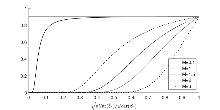
Figure 4.1: Worst-case asymptotic coverage probability of the conventional 90% VAR confidence interval. Horizontal axis: relative asymptotic standard deviation of LP vs. VAR. Different lines: different bounds $M$ on $\|\alpha(L)\|$. The solid horizontal line marks the nominal coverage probability $1-a=90\%$.

We conclude that, even for small amounts of VAR misspecification (as measured by the noise-to-signal ratio) and for relative estimator precisions of typical magnitudes, the scope for VAR undercoverage is material. This potential undercoverage may not be so concerning if the worst-case misspecification can be ruled out on economic theory grounds, or if it is easily detectable statistically. We now argue that neither appears to be the case.

Economic theory.

The shape and magnitude of the least favorable misspecification is difficult to rule out generally based on economic theory. The least favorable MA polynomial $\alpha^{\dagger}(L;h,M)=\sum_{\ell=1}^{\infty}\alpha_{\ell,h,M}^{\dagger}L^{\ell}$ for coverage is the same as the least favorable one for bias (i.e., the $\alpha(L)$ that achieves the maximum in Proposition 4.1). Since $\operatorname{aBias}(\hat{\delta}_{h})$ is linear in $\alpha(L)$, the least favorable choice given the constraint $\|\alpha(L)\|\leq M$ follows easily from the Cauchy-Schwarz inequality (see the proof of Proposition 4.1):

$$\alpha_{\ell,h,M}^{\dagger}\propto D^{1/2}H^{\prime}\Psi_{h}^{\prime}S^{-1}A^{\ell-1}HD^{1/2}-\mathbbm{1}(\ell\leq h)\sigma_{j^{*}}^{-1}D^{1/2}H^{\prime}(A^{\prime})^{h-\ell}e_{i^{*},n}e_{j^{*},m}^{\prime},\quad\ell=1,2,\dots,$$

where the constant of proportionality (which does not depend on the lag $\ell$) is chosen so that $\|\alpha^{\dagger}(L;h,M)\|=M$. Note that the shape of the least favorable MA polynomial depends on the particular horizon $h$ of interest but not on $M$; i.e., the bound $M^{2}/T$ on the noise-to-signal ratio only scales the polynomial up or down.

We note two main properties of the worst-case $\alpha_{\ell,h,M}^{\dagger}$. First, the magnitude of the MA coefficients decays exponentially as $\ell\to\infty$. In other words, not only is the overall magnitude of the least favorable model misspecification small (as imposed in the noise-to-signal bound), the MA coefficients at long lags are particularly small. Second, numerical examples shown in Section A.1 suggest that the MA coefficients tend to be largest in magnitude at horizon $h$, displaying either a hump-shaped pattern as a function of $\ell$—consistent with economic theories of adjustment costs or learning—or a single zig-zag pattern—consistent with theories of overshooting or lumpy adjustment. In fact, as we will show formally in Section 5.2, simple canonical models like an ARMA(1,1) map into misspecification polynomials $\alpha(L)$ that look extremely similar to the worst-case misspecification $\alpha^{\dagger}(L)$. We thus view MA dynamics of the worst-case form as empirically and theoretically realistic types of misspecification.

Statistical tests.

The least favorable misspecification is also difficult to detect statistically. Propositions 3.3 and 4.1 imply that, for $\alpha(L)=\alpha^{\dagger}(L;h,M)$, the asymptotic rejection probability of the Hausman test of correct VAR specification equals $r(M;z_{1-a/2})$. When $M=1$ (corresponding to a noise-to-signal ratio of $1/T$), the odds of the Hausman test failing to reject the misspecification are nearly 3-to-1 at significance level $a=10\%$, since $r(1;z_{0.95})=26\%$. At significance level $a=5\%$, the odds are nearly 5-to-1, since $r(1;z_{0.975})=17\%$. Standard ex post model misspecification tests are thus unlikely to indicate a problem even if the potential for undercoverage is severe.

Rather than committing a priori to a parameter space for $\alpha(L)$ through choice of $M$, we can also ask a different question: over all possible types and magnitudes of misspecification, what is the worst-case probability that the conventional VAR confidence interval fails to cover the true impulse response, yet we fail to reject correct specification of the VAR model?

Corollary 4.4.

Impose Assumption 3.1, $\zeta=1/2$, and $\operatorname{aVar}(\hat{\beta}_{h})>\operatorname{aVar}(\hat{\delta}_{h})>0$. Consider the joint event $\mathcal{A}_{T}$ that $\theta_{h,T}\notin\operatorname{CI}(\hat{\delta}_{h})$ and the Hausman test in Proposition 3.3 fails to reject misspecification. Then

$$\sup_{\alpha(L)}\;\lim_{T\to\infty}P(\mathcal{A}_{T})=\sup_{b\geq 0}\;r(b;z_{1-a/2})\left\{1-r\left(\frac{b}{\sqrt{\operatorname{aVar}(\hat{\beta}_{h})/\operatorname{aVar}(\hat{\delta}_{h})-1}};z_{1-a/2}\right)\right\},$$

where the supremum on the left-hand side is taken over all absolutely summable lag polynomials $\alpha(L)$.

Proof.

See Section C.6. ∎

Figure 4.2 plots this worst-case probability for significance level $a=10\%$, which as we have seen depends only on the ratio $\operatorname{aVar}(\hat{\delta}_{h})/\operatorname{aVar}(\hat{\beta}_{h})$. Under correct specification, the probability of the joint event is equal to $a(1-a)$ ($=9\%$ when $a=10\%$). Yet we see that the joint probability can exceed 46% when the asymptotic standard deviation of the VAR estimator is less than half that of the LP estimator. As $\operatorname{aVar}(\hat{\delta}_{h})/\operatorname{aVar}(\hat{\beta}_{h})\to 0$, the worst-case joint probability approaches $1-a$. We thus again see that statistical tests fail to guard researchers adequately against the potential for severe VAR coverage distortions.

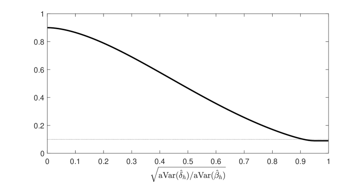
Figure 4.2: Worst-case asymptotic probability of the joint event that the conventional VAR confidence interval fails to cover the true impulse response and yet the Hausman test fails to reject misspecification. Horizontal axis: relative asymptotic standard deviation of LP vs. VAR. The dotted horizontal line marks the nominal significance level $a=10\%$.

4.4 Bias-aware inference

To fix the under-coverage of the conventional VAR confidence interval, we can adjust the critical value upward to compensate for the bias, as suggested in a general setting by Armstrong and Kolesár (2021). Suppose again that we restrict the misspecification $\alpha(L)$ to satisfy $\|\alpha(L)\|\leq M$. Then we define the bias-aware VAR confidence interval

$$\operatorname{CI}_{B}(\hat{\delta}_{h};M)\equiv\left[\hat{\delta}_{h}\pm\operatorname{cv}_{1-a}\left(M\sqrt{\frac{\operatorname{aVar}(\hat{\beta}_{h})}{\operatorname{aVar}(\hat{\delta}_{h})}-1}\right)\sqrt{\operatorname{aVar}(\hat{\delta}_{h})/T}\right],$$

where the bias-aware critical value $\operatorname{cv}_{1-a}(b)$ is given by the number such that $r(b;\operatorname{cv}_{1-a}(b))=a$, and $r(\cdot,\cdot)$ is defined in 3.2. By construction, this bias-aware confidence interval has correct (but potentially conservative) asymptotic coverage.

Corollary 4.5.

Impose Assumption 3.1, $\zeta=1/2$, and $\operatorname{aVar}(\hat{\delta}_{h})>0$. Then

$$\inf_{\alpha(L)\colon\|\alpha(L)\|\leq M}\lim_{T\to\infty}P(\theta_{h,T}\in\operatorname{CI}_{B}(\hat{\delta}_{h};M))=1-a.$$

Proof.

The result follows immediately from Propositions 3.2 and 4.1. ∎

A very tight bound $M$ on the signal-to-noise ratio is required for the bias-aware VAR interval to be shorter than the LP interval. The ratio of the length of the bias-aware interval to that of the conventional LP interval is a function only of $M$ and the asymptotic relative precision of LP and VAR. Figure 4.3 plots the relative interval length as a function of the relative asymptotic standard deviation, for significance level $a=10\%$ and for different misspecification bounds $M$. The figure shows that $M$ has to be quite small—apparently below 1—for the bias-aware VAR length to dominate the LP length regardless of the DGP and horizon. Even for $M=1.5$, bias-aware VAR is at best only moderately shorter than LP (and sometimes longer). For values of $M$ above 2 (corresponding to a noise-to-signal ratio above $4/T$), bias-aware VAR is dominated by LP.

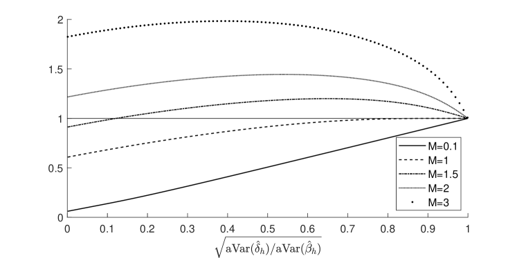
Figure 4.3: Relative length of bias-aware VAR confidence interval vs. conventional LP interval. Significance level $a=10\%$. Horizontal axis: relative asymptotic standard deviation of LP vs. VAR. Different lines: different bounds $M$ on $\|\alpha(L)\|$. The solid horizontal line marks the value 1.

In Section A.2 we show that the conventional LP confidence interval is at most slightly wider than a more efficient bias-aware confidence interval centered at the model averaging estimator $\hat{\theta}_{h}(\omega)=\omega\hat{\beta}_{h}+(1-\omega)\hat{\delta}_{h}$ introduced in 4.2 above. Even if the weight $\omega$ is chosen to optimize confidence interval length, the gains relative to the LP interval are very small when $M\geq 2$ (corresponding to a noise-to-signal ratio above $4/T$).

We conclude that, while bias-aware VAR inference is possible in theory, in practice the gains relative to the simpler LP interval are small at best, unless we put an extremely tight bound on the noise-to-signal ratio.

5 Simulations

In this section we show that our asymptotic results accurately reflect the finite-sample properties of LP and VAR procedures. The first set of simulations pertain to a simple ARMA(1,1) model, while the second set uses the popular structural macroeconomic model of Smets and Wouters (2007). Additional simulation results are reported in LABEL:app:sim_details.

5.1 Deriving the VARMA representation

We first show how we transform any given simulation DGP into the VARMA form assumed in Sections 3 and 4. The DGPs we consider have a vector MA representation

$$y_{t}=C(L)u_{t},$$ (5.1)

where $C(L)=I+\sum_{\ell=1}^{\infty}C_{\ell}L^{\ell}$, and $u_{t}$ is white noise with $\Sigma_{u}\equiv E(u_{t}u_{t}^{\prime})$. Given a choice of autoregressive lag length $p$, we seek to represent this process in VARMA($p,\infty$) form with MA component that is as small as possible. To this end, consider a linear least-squares projection of $y_{t}$ onto $p$ of its lags. We write the projection coefficients as $A_{\ell}(p)$, $\ell=1,2,\dots,p$, and define $A(L;p)\equiv I-\sum_{\ell=1}^{p}A_{\ell}(p)$. Letting $\tilde{C}(L;p)=\sum_{\ell=0}^{\infty}\tilde{C}_{\ell}(p)L^{\ell}\equiv A(L;p)C(L)$, equation (5.1) implies the VARMA($p,\infty$) representation

$$y_{t}=\sum_{\ell=1}^{p}A_{\ell}(p)y_{t-\ell}+\sum_{\ell=0}^{\infty}\tilde{C}_{\ell}(p)u_{t-\ell}.$$ (5.2)

Given a choice of $T$ as well as $\zeta$, it is straightforward to translate the representation given in (5.2) into our baseline form (3.1). We have thus arrived at a local-to-SVAR($p$) model that perfectly matches the second-moment properties of the original process $\{y_{t}\}$ in (5.1). The MA residual in (5.2) then measures the magnitude of the departure of the DGP from the best-fitting VAR($p$) model. As is the case for many structural dynamic macro models, the simulation DGPs we consider below cannot be represented exactly as finite-order VAR models. Our results will shed light on whether the resulting MA components are large enough to meaningfully distort VAR inference in practice.

5.2 Illustrative univariate model

We begin with an illustration based on a simple univariate ARMA(1,1) model. The purpose of this section is threefold: first, to get a sense of possible magnitudes for the degree of VAR misspecification $M$; second, to compare the actual with the worst-case lag polynomial $\alpha(L)$ in a simple and transparent environment; and third, to provide a visual illustration of our main theoretical results.

Model.

We consider an ARMA(1,1) process:

$$y_{t}=\rho y_{t-1}+\varepsilon_{t}+\psi\varepsilon_{t-1},\quad\varepsilon_{t}\overset{i.i.d.}{\sim}N(0,\sigma^{2}).$$ (5.3)

Throughout this section we set $\rho=0.9$, $\sigma^{2}=1$, and $\psi\in\{0,0.25,0.5,0.75\}$. The lagged MA term thus accounts for up to 36 per cent of the overall variance of the error term in (5.3).

Results.

We first quantify the amount of misspecification. For a given lag length $p$ as well as reference values $T=240$ and $\zeta=1/2$, we can proceed as in Section 5.1 to translate the model (5.3) into an ARMA($p,\infty$) representation (5.2), with the AR parameters providing the best fit given $p$. Table 5.1 shows the total amount of MA misspecification $M\equiv||\alpha(L)||$ as a function of $p$ and $\psi$. The table also reports the quantity $M^{2}/(1+M^{2})$, the minimax optimal ex ante model averaging weight on LP in 4.2. As expected, shorter lag lengths $p$ or larger MA coefficients $\psi$ mean greater misspecification, in the sense of larger $M$. We also see that, even for moderate $p$ and $\psi$, the degree of misspecification—and accordingly the optimal LP weight—can be large.

	$M$			$\frac{M^{2}}{1+M^{2}}$
$p$	$\psi=0.25$	$\psi=0.50$	$\psi=0.75$	$\psi=0.25$	$\psi=0.50$	$\psi=0.75$
1	3.622	7.396	11.234	0.929	0.982	0.992
2	0.882	3.337	6.821	0.437	0.918	0.979
3	0.220	1.631	4.682	0.046	0.727	0.956
4	0.055	0.811	3.361	0.003	0.397	0.919

Table 5.1: $M$ and $\frac{M^{2}}{1+M^{2}}$ as a function of $p$ and $\psi$ in the ARMA(1,1) model (5.3), with the researcher estimating an AR($p$).

Next we show that, in this DGP, the implied misspecification polynomial $\alpha(L)$ can be very close to the theoretical least favorable polynomial $\alpha^{\dagger}(L;h)$ derived in Section 4.1, which represents the worst case for AR bias and coverage. Figure 5.1 shows $\alpha(L)$ (solid black) as well as $\alpha^{\dagger}(L;h)$ (colored, dashed and dotted) for horizons $h\in\{1,5,10\}$, and throughout setting $\psi=0.5$. For both $p=1$ as well as $p=4$, the actual MA polynomial $\alpha(L)$ implied by the ARMA(1,1) model (5.3) is very close—though not quite identical—to the worst-case $\alpha^{\dagger}(L;1)$ at horizon $h=1$. Hence, the least favorable lag polynomial is not some practically immaterial theoretical curiosity in the particular DGP considered here.

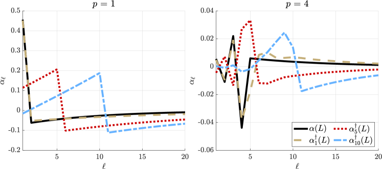
Figure 5.1: $\alpha(L)$ (black, solid) and least favorable $\alpha^{\dagger}(L)$ (colored, dashed and dotted) at various horizons for the simple ARMA(1,1) model (5.3), with the researcher estimating an AR($1$) (left) and an AR($4$) (right).

Finally, and consistent with our theory, we find that coverage can be poor for VAR confidence intervals, while LP intervals are robust to the presence of the MA term. Figure 5.2 reports coverage rates and median confidence interval lengths for the cases $\psi=0$ (no misspecification) and $\psi=0.25$ (moderate misspecification, with the lagged MA term accounting for around 6% of the variance of the error term). We throughout consider $p=1$, simulate 5,000 samples of size $T=240$, and then for each construct delta method as well as bootstrap LP and AR confidence intervals (assuming homoskedasticity), in blue and red, respectively. The top panel reveals that, when the AR(1) model is in fact correctly specified (i.e., for $\psi=0$), then both LP and AR confidence intervals attain the nominal coverage probability of 90 per cent (left panel); furthermore, and also as expected, the AR confidence intervals are meaningfully shorter (right panel). In the misspecified case in the bottom panel, the AR confidence intervals instead substantially undercover, and particularly so at short horizons. This is consistent with our general theoretical results as well as our observation above that the actual misspecification lag polynomial $\alpha(L)$ is close to the horizon-$1$ worst-case one, $\alpha^{\dagger}(L;1)$. We also see that LP, on the other hand, exhibits at worst mild undercoverage.

AR(1) – Correct Specification
ARMA(1,1), $\psi=0.25$

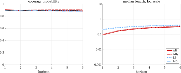
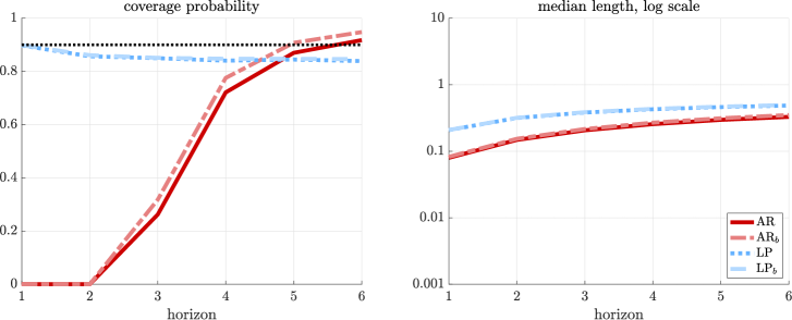
Figure 5.2: Coverage probabilities (left) and median confidence interval length (right) for AR (red) and LP (blue) for delta method and bootstrap (solid, dashed, and dotted). The DGP is (5.3) with $\psi=0$ (top) and $\psi=0.25$ (bottom), with estimation lag length fixed at $p=1$.

5.3 Misspecification in Smets and Wouters (2007)

For our quantitative simulation exercise, we take as the DGP the well-known structural macroeconomic model of Smets and Wouters (2007). This environment is ideal for our purposes, as it allows us to closely mimic applied macroeconometric practice: the model is rich enough to match well the second-moment properties of standard macroeconomic time series data, yet at the same time features the interpretable, structural shocks typically studied in applied work, like monetary or cost-push shocks.

Framework.

We consider the model of Smets and Wouters, solved at its (quarterly) posterior mode parameterization. The econometrician observes the wage cost-push shock, inflation, wages, and total hours worked. The impulse response function of interest is that of inflation with respect to the cost-push shock. Our specification follows recent work that studies the role of labor markets in the post-2021 inflation spike (e.g., Bernanke and Blanchard, 2023). Results for alternative set-ups with other structural shocks and different shock identification schemes are reported in LABEL:app:sim_details.

Results.

We begin by quantifying the amount of misspecification, having represented the model in VARMA form (see Section 5.1) for $T=240$ and $\zeta=1/2$. Table 5.2 shows the total degree of misspecification $M$ as well as the minimax MSE-optimal weight $M^{2}/(1+M^{2})$ on LP in 4.2 as a function of the VAR lag length $p$. As anticipated, the larger $p$, the smaller $M$. Importantly, however, $M$ only declines extremely slowly with the lag length $p$. In particular, for lag lengths typical in applied practice (for quarterly data), misspecification is material, with $M\approx 3.23$ for a standard lag length of $p=4$, and $M\approx 1.89$ even for a long lag length of $p=8$. This suggests that—depending on the shape of $\alpha(L)$—there is potential for misspecification to materially affect VAR inference.

$p$	$M$	$\frac{M^{2}}{1+M^{2}}$
1	34.053	0.999
2	5.412	0.967
4	3.225	0.912
8	1.893	0.782
12	1.324	0.637
20	0.915	0.456
40	0.614	0.274

Table 5.2: $M$ and $\frac{M^{2}}{1+M^{2}}$ as a function of $p$ in the structural model of Smets and Wouters (2007), with the researcher observing the cost-push shock, inflation, wages, and hours worked, and estimating a VAR($p$).

Lag length via AIC
Lag length $p=4$
Lag length $p=8$

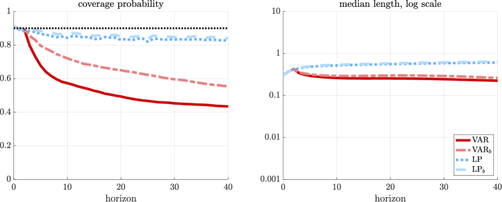
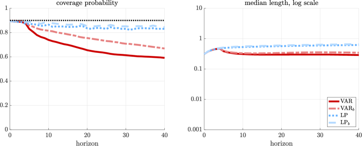
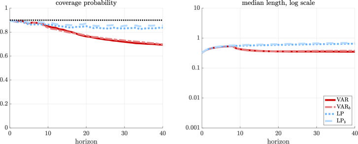
Figure 5.3: See Figure 5.2. The DGP is the model of Smets and Wouters, and the researcher estimates the response of inflation to an observed cost-push shock. Lag length $p$ is selected using the AIC for the top panel, and set to $p=4$ and $p=8$ for the middle and bottom panels, respectively.

Figure 5.3 shows that VAR confidence intervals indeed severely undercover, while LP intervals remain robust. We simulate 5,000 samples of size $T=240$, and for each construct delta method as well as bootstrap LP and VAR confidence intervals (assuming homoskedasticity). The top panel displays our headline results, with lag length $p$ selected using the AIC. At all but very short horizons, VAR confidence intervals materially undercover, while LP throughout attains close to the nominal coverage level, consistent with our theoretical results. We emphasize that these results for VAR inference are obtained even though the lag length $p$ is selected using the AIC: the median selected lag length is $p=2$, which here is evidently insufficient to guard against material VAR bias and undercoverage. The middle and bottom panels then further illustrate our “no free lunch” results. For those panels, we instead manually select longer lag lengths: $p=4$ for the middle panel and $p=8$ for the bottom panel. VAR coverage is now closer to the nominal level for all horizons $h\leq p$ (consistent with 3.3), but at the same time confidence intervals become essentially as wide as for LP. At longer horizons we obtain the same picture as before: material undercoverage for VAR, and coverage close to the nominal level for LP.

LABEL:app:sim_details shows that these conclusions extend to alternative shocks and alternative shock identification schemes. We there furthermore investigate what happens if the actual lag polynomial $\alpha(L)$ is replaced by the theoretical least favorable one. In that case, the magnitudes of VAR undercoverage are broadly comparable with those obtained under the actual $\alpha(L)$ implied by the Smets and Wouters (2007) model, revealing that the least favorable MA polynomial $\alpha^{\dagger}(L,\cdot)$ is not particularly pathological, echoing our earlier finding in the univariate ARMA(1,1) simulation DGP.

Summary.

The simulation results in this section suggest that our theoretical results are likely to have practical bite. In empirically realistic settings, LP confidence intervals have close-to-nominal coverage, while VAR misspecification is plausibly large enough (and similar enough to the worst-case misspecification) to cause severe VAR coverage distortions. A researcher may guard against such distortions by increasing the lag length beyond the values suggested by standard information criteria; however, in doing so, she will end up with confidence intervals of length comparable to those of LPs.

6 Conclusion

We have shown that, while conventional LP inference is robust to surprisingly large amounts of misspecification, VAR inference is much more fragile. Conventional VAR confidence intervals suffer from severe coverage distortions even for misspecification that is small, difficult to rule out ex ante using economic theory, and difficult to detect ex post with VAR model specification tests. These analytical results demonstrate that—when the goal is to construct valid confidence intervals for impulse responses, as opposed to minimizing MSE—the smaller bias of LPs documented in simulations by Li, Plagborg-Møller, and Wolf (2024) is more valuable than the smaller variance enjoyed by VAR estimators.

A practical take-away for LP analysis is that researchers should control for lags of the data that are strong predictors of the outcome and impulse variables. This is important even if the researcher directly observes a near-perfect proxy for the shock of interest. However, it is not necessary to get the lag length exactly right to achieve correct coverage, and conventional information criteria (such as AIC) suffice to select an appropriate lag length for LP in our framework. Our results complement the finding of Montiel Olea and Plagborg-Møller (2021) that lag-augmented LP confidence intervals are also more robust than VAR intervals to persistence in the data and to the length of the impulse response horizon.

Is there a way forward for VAR inference? The conventional VAR confidence interval is valid if the estimation lag length is sufficiently large, but our results show that this can only happen by making the interval equivalent with the LP interval. Using a smaller lag length combined with a bias-aware critical value typically leads to wider confidence intervals than LP. Another option would be to estimate VARMA models rather than pure VARs, though this would be computationally expensive, and the bias-variance trade-off relative to LPs is unclear. In principle, VAR procedures may work better under additional restrictions on the misspecification, such as shape restrictions on the impulse response functions. However, it appears that detailed application-specific restrictions would be required to generate a negligible worst-case bias, since we have shown that the least favorable misspecification in our baseline analysis is economically realistic. Rather than restricting the parameter space, an alternative would be to weaken the coverage requirement, e.g., only requiring a certain coverage probability on average over a set of horizons (Armstrong, Kolesár, and Plagborg-Møller, 2022), or by changing the target for inference from the true impulse response function to a smooth projection of this function (Genovese and Wasserman, 2008). Finally, a subjectivist Bayesian VAR modeler need only worry about our negative results if their prior on potential misspecification attaches significant weight to MA processes that imply large VAR biases.

Appendix A Further theoretical results

A.1 Least favorable misspecification

Figure A.1 plots some numerical examples of the least favorable MA polynomial $\alpha^{\dagger}(L;h,M)=\sum_{\ell=1}^{\infty}\alpha^{\dagger}_{\ell,h,M}L^{\ell}$ discussed in Section 4.3. We focus here on the univariate local-to-AR(1) model from Section 2, though unreported numerical experiments suggest that the qualitative features mentioned below also apply to multivariate models. Recall that the least favorable MA coefficients depend on the horizon $h$ of interest, while $M$ only influences the overall scale of the coefficients, and not their shape as a function of the lag $\ell$. The figure shows that the shape of the coefficients either takes the form of a hump or a single zig-zag pattern, with the largest absolute value of the coefficients generally occurring at $\ell=h$. Notice that we can flip the signs of all coefficients without changing the bias.

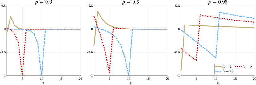
Figure A.1: Least favorable $\alpha^{\dagger}(L;h)$ for horizons $h\in\{1,5,10\}$ for local-to-AR(1) models with different persistence parameters $\rho$ (left, middle, and right panel).

A.2 More efficient bias-aware confidence interval

Generalizing the bias-aware VAR confidence interval in Section 4.4, consider a bias-aware confidence interval that is centered at the model averaging estimator $\hat{\theta}_{h}(\omega)=\omega\hat{\beta}_{h}+(1-\omega)\hat{\delta}_{h}$ from 4.2:

$$\operatorname{CI}_{B}(\hat{\theta}_{h}(\omega);M)\equiv\left[\hat{\theta}_{h}(\omega)\pm\operatorname{cv}_{1-a}\left(\frac{(1-\omega)M\lambda}{\sqrt{1+\omega^{2}\lambda^{2}}}\right)\sqrt{(1+\omega^{2}\lambda^{2})\operatorname{aVar}(\hat{\delta}_{h})/T}\right],$$

where $\lambda\equiv\sqrt{\operatorname{aVar}(\hat{\beta}_{h})/\operatorname{aVar}(\hat{\delta}_{h})-1}$. This interval equals the conventional LP interval when $\omega=1$ and the bias-aware VAR interval when $\omega=0$.

Corollary A.1.

Impose Assumption 3.1, $\zeta=1/2$, and $\operatorname{aVar}(\hat{\delta}_{h})>0$. Then, for any $\omega\in[0,1]$,

$$\inf_{\alpha(L)\colon\|\alpha(L)\|\leq M}\lim_{T\to\infty}P(\theta_{h,T}\in\operatorname{CI}_{B}(\hat{\theta}_{h}(\omega);M))=1-a.$$

Proof.

The result follows from Propositions 3.1, 3.2, 3.1 and 4.1 and the same calculations as in the proof of 4.2. ∎

If we choose the weight $\omega$ to minimize confidence interval length, the resulting bias-aware interval tends to be nearly as long as the LP interval. The length-optimal averaging weight $\omega=\omega^{*}$ is given by

$$\omega^{*}\equiv\operatorname*{argmin}_{\omega\in[0,1]}\;\operatorname{cv}_{1-a}\left(\frac{(1-\omega)M\lambda}{\sqrt{1+\omega^{2}\lambda^{2}}}\right)\sqrt{1+\omega^{2}\lambda^{2}}.$$

Figure A.3 shows this optimal weight as a function of $M$ and the relative asymptotic standard deviation of the VAR and LP estimators, while Figure A.3 shows the length of the resulting optimal bias-aware confidence interval relative to the length of the conventional LP interval. We see that, for $M\geq 2$, there is little gain from reporting the optimal bias-aware interval rather than the LP interval, regardless of the relative precision of VAR and LP. An additional observation is that, for $M\geq 2$, the length-optimal $\omega^{*}$ is numerically close to the MSE-optimal weight $M^{2}/(1+M^{2})$ derived in 4.2.

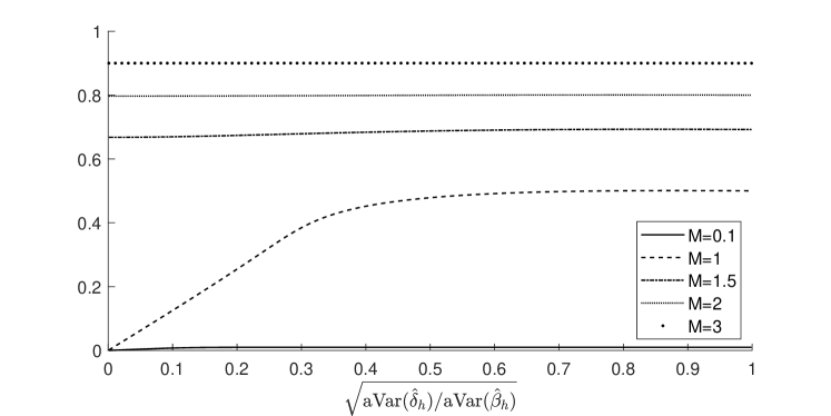
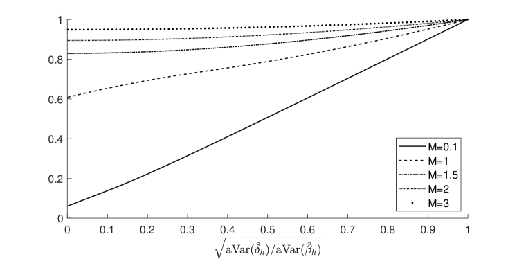
Figure A.2: Length-optimal weight on LP in bias-aware confidence interval. Significance level $a=10\%$. Horizontal axis: relative asymptotic standard deviation of LP vs. VAR. Different lines: different bounds $M$ on $\|\alpha(L)\|$.

Figure A.3: Relative length of optimal bias-aware confidence interval vs. conventional LP interval. Significance level $a=10\%$. Horizontal axis: relative asymptotic standard deviation of LP vs. VAR. Different lines: different bounds $M$ on $\|\alpha(L)\|$.

Appendix B Proofs of propositions

B.1 Proof of Proposition 3.1

LABEL:thm:lp_coefficients_aux shows that we can represent

$$y_{i^{*},t+h}=\theta_{h,T}\varepsilon_{j^{*},t}+\underline{B}_{h,y}^{\prime}\underline{y}_{j^{*},t}+B_{h,y}^{\prime}y_{t-1}+\xi_{h,i^{*},t}+T^{-\zeta}\Theta_{h}(L)\varepsilon_{t},$$ (B.1)

where the precise expressions for the coefficient matrices are given in LABEL:thm:lp_coefficients_aux. The lemma also shows that the $1\times n$ two-sided lag polynomial $\Theta_{h}(L)=\sum_{\ell=-\infty}^{\infty}\Theta_{h,\ell}L^{\ell}$ is absolutely summable and satisfies $\Theta_{h,0,j^{*}}=0$. That is, $\Theta_{h}(L)\varepsilon_{t}$ is independent of $\varepsilon_{j^{*},t}$ (but not of $\varepsilon_{j^{*},s}$ for $s\neq t$).

Let $\hat{x}_{h,t}$ be the residual in a regression of $y_{j^{*},t}$ on $\underline{y}_{j^{*},t}$ and $y_{t-1}$. By definition, $\hat{x}_{h,t}$ is in-sample orthogonal to $\underline{y}_{j^{*},t}$ and $y_{t-1}$. Hence,

$$\hat{\beta}_{h} =\frac{\sum_{t=1}^{T-h}y_{i^{*},t+h}\hat{x}_{h,t}}{\sum_{t=1}^{T-h}\hat{x}_{h,t}^{2}}$$

$$=\theta_{h,T}+\frac{\sum_{t=1}^{T-h}(y_{i^{*},t+h}-\theta_{h,T}\hat{x}_{h,t}-\underline{B}_{h,y}^{\prime}\underline{y}_{j^{*},t}-B_{h,y}^{\prime}y_{t-1})\hat{x}_{h,t}}{\sum_{t=1}^{T-h}\hat{x}_{h,t}^{2}}\quad\text{by orthogonality}$$

$$=\theta_{h,T}+\frac{T^{-1}\sum_{t=1}^{T-h}(y_{i^{*},t+h}-\theta_{h,T}\hat{x}_{h,t}-\underline{B}_{h,y}^{\prime}\underline{y}_{j^{*},t}-B_{h,y}^{\prime}y_{t-1})\hat{x}_{h,t}}{\sigma_{j^{*}}^{2}+o_{p}(1)}\quad\text{by \lx@cref{creftype~refnum}{thm:x}(\ref{itm:thm_x_ii})}$$

$$=\theta_{h,T}+\frac{T^{-1}\sum_{t=1}^{T-h}(y_{i^{*},t+h}-\theta_{h,T}\varepsilon_{j^{*},t}-\underline{B}_{h,y}^{\prime}\underline{y}_{j^{*},t}-B_{h,y}^{\prime}y_{t-1})\hat{x}_{h,t}+o_{p}(T^{-1/2})}{\sigma_{j^{*}}^{2}+o_{p}(1)}\quad\text{by \lx@cref{creftype~refnum}{thm:x}(\ref{itm:thm_x_iii})}$$

$$=\theta_{h,T}+\frac{T^{-1}\sum_{t=1}^{T-h}(\xi_{h,i^{*},t}+T^{-\zeta}\Theta_{h}(L)\varepsilon_{t})\hat{x}_{h,t}}{\sigma_{j^{*}}^{2}+o_{p}(1)}+o_{p}(T^{-1/2})\quad\text{by \eqref{eqn:lp_repr}}$$

$$=\theta_{h,T}+\frac{T^{-1}\sum_{t=1}^{T-h}(\xi_{h,i^{*},t}+T^{-\zeta}\Theta_{h}(L)\varepsilon_{t})\varepsilon_{j^{*},t}+o_{p}(T^{-1/2})+O_{p}(T^{-2\zeta}+T^{-1/2-\zeta})}{\sigma_{j^{*}}^{2}+o_{p}(1)}+o_{p}(T^{-1/2})$$

by LABEL:thm:x(LABEL:itm:thm_x_iv) and (LABEL:itm:thm_x_v)

$$=\theta_{h,T}+\frac{T^{-1}\sum_{t=1}^{T-h}(\xi_{h,i^{*},t}+T^{-\zeta}\Theta_{h}(L)\varepsilon_{t})\varepsilon_{j^{*},t}}{\sigma_{j^{*}}^{2}+o_{p}(1)}+o_{p}(T^{-1/2}).$$

Finally, LABEL:thm:lp_coefficients_aux shows that

$$T^{-1}\sum_{t=1}^{T-h}(\Theta_{h}(L)\varepsilon_{t})\varepsilon_{j^{*},t}=O_{p}(T^{-1/2}).$$

Thus, we conclude that

$$T^{-1}\sum_{t=1}^{T-h}T^{-\zeta}(\Theta_{h}(L)\varepsilon_{t})\varepsilon_{j^{*},t}=O_{p}(T^{-1/2-\zeta})=o_{p}(T^{-1/2}),$$

which completes the proof. ∎

B.2 Proof of Proposition 3.2

Note first that

$$\hat{\delta}_{h}-e_{i^{*},n}^{\prime}A^{h}H_{\bullet,j^{*}} =e_{i^{*},n}^{\prime}\hat{A}^{h}\hat{\nu}-e_{i^{*},n}^{\prime}A^{h}H_{\bullet,j^{*}}$$

$$=e_{i^{*},n}^{\prime}\hat{A}^{h}H_{\bullet,j^{*}}-e_{i^{*},n}^{\prime}A^{h}H_{\bullet,j^{*}}+e_{i^{*},n}^{\prime}\hat{A}^{h}(\hat{\nu}-H_{\bullet,j^{*}}).$$

LABEL:thm:A shows that $\hat{A}-A=O_{p}(T^{-\zeta}+T^{-1/2})$. Since it is known that

$$\left(\frac{\partial(e_{i^{*},n}^{\prime}A^{h}H_{\bullet,j^{*}})}{\partial\operatorname*{vec}(A)}\right)^{\prime}=(H_{\bullet,j^{*}}^{\prime}\otimes e_{i^{*},n}^{\prime})\left(\sum_{\ell=1}^{h}(A^{\prime})^{h-\ell}\otimes A^{\ell-1}\right)=\sum_{\ell=1}^{h}H_{\bullet,j^{*}}^{\prime}(A^{\prime})^{h-\ell}\otimes e_{i^{*},n}^{\prime}A^{\ell-1},$$

see for example Magnus and Neudecker (2007, Table 7, p. 208), the delta method gives

$$\hat{\delta}_{h}-e_{i^{*},n}^{\prime}A^{h}H_{\bullet,j^{*}} =\left(\sum_{\ell=1}^{h}H_{\bullet,j^{*}}^{\prime}(A^{\prime})^{h-\ell}\otimes e_{i^{*},n}^{\prime}A^{\ell-1}\right)\operatorname*{vec}(\hat{A}-A)+e_{i^{*},n}^{\prime}A^{h}(\hat{\nu}-H_{\bullet,j^{*}})+o_{p}(T^{-\zeta}+T^{-1/2})$$

$$=\sum_{\ell=1}^{h}e_{i^{*},n}^{\prime}A^{\ell-1}(\hat{A}-A)A^{h-\ell}H_{\bullet,j^{*}}+e_{i^{*},n}^{\prime}A^{h}(\hat{\nu}-H_{\bullet,j^{*}})+o_{p}(T^{-\zeta}+T^{-1/2})$$

$$=\operatorname*{trace}\left\{\Psi_{h}(\hat{A}-A)\right\}+e_{i^{*},n}^{\prime}A^{h}(\hat{\nu}-H_{\bullet,j^{*}})+o_{p}(T^{-\zeta}+T^{-1/2}),$$

where $\Psi_{h}\equiv\sum_{\ell=1}^{h}A^{h-\ell}H_{\bullet,j^{*}}e_{i^{*},n}^{\prime}A^{\ell-1}$. LABEL:thm:A further implies that

$$\operatorname*{trace}\left\{\Psi_{h}(\hat{A}-A)\right\} =T^{-\zeta}\operatorname*{trace}\left\{S^{-1}\Psi_{h}H\sum_{\ell=1}^{\infty}\alpha_{\ell}DH^{\prime}(A^{\prime})^{\ell-1}\right\}$$

$$+\operatorname*{trace}\left\{S^{-1}\Psi_{h}HT^{-1}\sum_{t=1}^{T}\varepsilon_{t}\tilde{y}_{t-1}^{\prime}\right\}+o_{p}(T^{-\zeta}),$$

where $S$ was defined in Assumption 3.1. LABEL:thm:nu shows that

$$\hat{\nu}-H_{\bullet,j^{*}}=\frac{1}{\sigma_{j^{*}}^{2}}T^{-1}\sum_{t=1}^{T}\xi_{0,t}\varepsilon_{j^{*},t}+o_{p}(T^{-1/2}).$$

Define

$$\operatorname{aBias}(\hat{\delta}_{h})\equiv\operatorname*{trace}\left\{S^{-1}\Psi_{h}H\sum_{\ell=1}^{\infty}\alpha_{\ell}DH^{\prime}(A^{\prime})^{\ell-1}\right\}-e_{i^{*},n}^{\prime}\sum_{\ell=1}^{h}A^{h-\ell}H\alpha_{\ell}e_{j^{*},m}.$$

Using the definition of $\theta_{h,T}$ and re-arranging terms gives the desired result. ∎

B.3 Proof of Proposition 3.3

By Propositions 3.1 and 3.2 and 3.1,

$$\hat{\beta}_{h}-\hat{\delta}_{h} =-T^{-\zeta}\operatorname{aBias}(\hat{\delta}_{h})+R_{T}+o_{p}(T^{-\zeta}+T^{-1/2}),$$

where

$$\sqrt{T}R_{T}\overset{d}{\to}N(0,\operatorname{aVar}(\hat{\beta}_{h})-\operatorname{aVar}(\hat{\delta}_{h})).$$

Consider the following three cases:

1. $\zeta\in(1/4,1/2)$: In this case

   $$\lim_{T\to\infty}P\left(\frac{\sqrt{T}|\hat{\beta}_{h}-\hat{\delta}_{h}|}{\sqrt{\operatorname{aVar}(\hat{\beta}_{h})-\operatorname{aVar}(\hat{\delta}_{h})}}>z_{1-a/2}\right) =\lim_{T\to\infty}P\left(\frac{T^{\zeta}|\hat{\beta}_{h}-\hat{\delta}_{h}|}{\sqrt{\operatorname{aVar}(\hat{\beta}_{h})-\operatorname{aVar}(\hat{\delta}_{h})}}>\frac{z_{1-a/2}}{T^{1/2-\zeta}}\right)$$

   $$=P\left(\frac{|\operatorname{aBias}(\hat{\delta}_{h})|}{\sqrt{\operatorname{aVar}(\hat{\beta}_{h})-\operatorname{aVar}(\hat{\delta}_{h})}}>0\right)$$

   $$=1.$$

   where the last inequality uses the fact that $\operatorname{aBias}(\hat{\delta}_{h})\neq 0$.

2. $\zeta>1/2$: In this case

   $$\sqrt{T}(\hat{\beta}_{h}-\hat{\delta}_{h})\overset{d}{\to}N(0,\operatorname{aVar}(\hat{\beta}_{h})-\operatorname{aVar}(\hat{\delta}_{h})),$$

   and thus

   $$\lim_{T\to\infty}P\left(\frac{\sqrt{T}|\hat{\beta}_{h}-\hat{\delta}_{h}|}{\sqrt{\operatorname{aVar}(\hat{\beta}_{h})-\operatorname{aVar}(\hat{\delta}_{h})}}>z_{1-a/2}\right)=a.$$

3. $\zeta=1/2$: In this case

   $$\sqrt{T}(\hat{\beta}_{h}-\hat{\delta}_{h})\overset{d}{\to}N(\operatorname{aBias}(\hat{\delta}_{h}),\operatorname{aVar}(\hat{\beta}_{h})-\operatorname{aVar}(\hat{\delta}_{h})).$$

   Thus,

   $$\lim_{T\to\infty}P\left(\frac{\sqrt{T}|\hat{\beta}_{h}-\hat{\delta}_{h}|}{\sqrt{\operatorname{aVar}(\hat{\beta}_{h})-\operatorname{aVar}(\hat{\delta}_{h})}}>z_{1-a/2}\right)=r\left(\frac{b_{h}}{\sqrt{\operatorname{aVar}(\hat{\beta}_{h})/\operatorname{aVar}(\hat{\delta}_{h})-1}};z_{1-a/2}\right),$$

   where $b_{h}\equiv\operatorname{aBias}(\hat{\delta}_{h})/\sqrt{\operatorname{aVar}(\hat{\delta}_{h})}$ and $r(b;c)\equiv P_{Z\sim N(0,1)}(|Z+b|>c)=\Phi(-c-b)+\Phi(-c+b)$, as in 3.2.

In summary, the three cases above show that

$$\lim_{T\to\infty}P\left(\frac{\sqrt{T}|\hat{\beta}_{h}-\hat{\delta}_{h}|}{\sqrt{\operatorname{aVar}(\hat{\beta}_{h})-\operatorname{aVar}(\hat{\delta}_{h})}}>z_{1-a/2}\right)=\lim_{T\to\infty}r\left(\frac{T^{1/2-\zeta}b_{h}}{\sqrt{\operatorname{aVar}(\hat{\beta}_{h})/\operatorname{aVar}(\hat{\delta}_{h})-1}};z_{1-a/2}\right).\qed$$

B.4 Proof of Proposition 4.1

Rewrite the numerator of $b_{h}$ as

$$\operatorname*{trace}\left\{S^{-1}\Psi_{h}H\sum_{\ell=1}^{\infty}\alpha_{\ell}DH^{\prime}(A^{\prime})^{\ell-1}\right\}-e_{i^{*},n}^{\prime}\sum_{\ell=1}^{h}A^{h-\ell}H\alpha_{\ell}e_{j^{*},m}=\sum_{\ell=1}^{\infty}\operatorname*{trace}\left\{\Xi_{h,\ell}D^{-1/2}\alpha_{\ell}D^{1/2}\right\},$$

with

$$\Xi_{h,\ell}\equiv D^{1/2}H^{\prime}(A^{\prime})^{\ell-1}S^{-1}\Psi_{h}HD^{1/2}-\mathbbm{1}(\ell\leq h)D^{-1/2}e_{j^{*},m}e_{i^{*},n}^{\prime}A^{h-\ell}HD^{1/2}.$$

By Cauchy-Schwarz, we can bound the squared value of the numerator of $b_{h}$ as follows:

$$\left(\sum_{\ell=1}^{\infty}\operatorname*{trace}\left\{\Xi_{h,\ell}D^{-1/2}\alpha_{\ell}D^{1/2}\right\}\right)^{2} \leq\left(\sum_{\ell=1}^{\infty}\operatorname*{trace}(\Xi_{h,\ell}^{\prime}\Xi_{h,\ell})\right)$$

$$\qquad\times\underbrace{\left(\sum_{\ell=1}^{\infty}\operatorname*{trace}\{(D^{-1/2}\alpha_{\ell}D^{1/2})^{\prime}D^{-1/2}\alpha_{\ell}D^{1/2}\}\right)}_{=\|\alpha(L)\|^{2}}.$$

Moreover, the bound is achieved by choosing $\alpha_{\ell}\propto\Xi_{h,\ell}^{\prime}$ for $\ell=1,2,\dots$. Hence, the statement of the proposition follows if we can show that

$$\sum_{\ell=1}^{\infty}\operatorname*{trace}(\Xi_{h,\ell}^{\prime}\Xi_{h,\ell})=\operatorname{aVar}(\hat{\beta}_{h})-\operatorname{aVar}(\hat{\delta}_{h}).$$

Indeed, by multiplying out terms and using $\Sigma=HDH^{\prime}$, we obtain

$$\sum_{\ell=1}^{\infty}\operatorname*{trace}(\Xi_{h,\ell}^{\prime}\Xi_{h,\ell}) =\sum_{\ell=1}^{\infty}\operatorname*{trace}(A^{\ell-1}\Sigma(A^{\prime})^{\ell-1}S^{-1}\Psi_{h}\Sigma\Psi_{h}^{\prime}S^{-1})$$

$$\quad-2\sum_{\ell=1}^{h}\operatorname*{trace}(A^{\ell-1}H_{\bullet,j^{*}}e_{i^{*},n}^{\prime}A^{h-\ell}\Sigma\Psi_{h}^{\prime}S^{-1})$$

$$\quad+\sum_{\ell=1}^{h}\sigma_{j^{*}}^{-2}e_{i^{*},n}^{\prime}A^{h-\ell}\Sigma(A^{\prime})^{h-\ell}e_{i^{*},n}.$$

The first term on the right-hand side above equals

$$\operatorname*{trace}\bigg{\{}\underbrace{\left(\sum_{\ell=1}^{\infty}A^{\ell-1}\Sigma(A^{\prime})^{\ell-1}\right)}_{=\operatorname*{Var}(\tilde{y}_{t})=S}S^{-1}\Psi_{h}\Sigma\Psi_{h}^{\prime}S^{-1}\bigg{\}}=\operatorname*{trace}\{\Psi_{h}\Sigma\Psi_{h}^{\prime}S^{-1}\}.$$

The second term on the right-hand side two displays ago equals

$$-2\operatorname*{trace}\bigg{\{}\underbrace{\left(\sum_{\ell=1}^{h}A^{\ell-1}H_{\bullet,j^{*}}e_{i^{*},n}^{\prime}A^{h-\ell}\right)}_{=\sum_{\ell=1}^{h}A^{h-\ell}H_{\bullet,j^{*}}e_{i^{*},n}^{\prime}A^{\ell-1}=\Psi_{h}}\Sigma\Psi_{h}^{\prime}S^{-1}\bigg{\}}=-2\operatorname*{trace}\{\Psi_{h}\Sigma\Psi_{h}^{\prime}S^{-1}\}.$$

We have shown

$$\sum_{\ell=1}^{\infty}\operatorname*{trace}(\Xi_{h,\ell}^{\prime}\Xi_{h,\ell})=\frac{1}{\sigma_{j^{*}}^{2}}\sum_{\ell=1}^{h}e_{i^{*},n}^{\prime}A^{h-\ell}\Sigma(A^{\prime})^{h-\ell}e_{i^{*},n}-\operatorname*{trace}\{\Psi_{h}\Sigma\Psi_{h}^{\prime}S^{-1}\},$$

which in turn equals $\operatorname{aVar}(\hat{\beta}_{h})-\operatorname{aVar}(\hat{\delta}_{h})$ (cf. 3.1), as required. ∎

Appendix C Proofs of corollaries

C.1 Proof of 3.1

By Proposition 3.1 and the that fact $\xi_{h,i^{*},t}\varepsilon_{j^{*},t}$ is serially uncorrelated, the asymptotic variance of LP equals $\sigma_{j^{*}}^{-4}E[\xi_{h,i^{*},t}^{2}\varepsilon_{j^{*},t}^{2}]=\sigma_{j^{*}}^{-2}E[\xi_{h,i^{*},t}^{2}]$, where $\xi_{h,i^{*},t}$ is the $i^{*}$-th element of the $n\times 1$ vector

$$\xi_{h,t}=(\xi_{h,1,t},\dots,\xi_{h,n,t})^{\prime}\equiv A^{h}\overline{H}_{j^{*}}\overline{\varepsilon}_{j^{*},t}+\sum_{\ell=1}^{h}A^{h-\ell}H\varepsilon_{t+\ell},$$

with $\overline{H}_{j^{*}}\equiv(H_{\bullet,j^{*}+1},\dots,H_{\bullet,m})$ and $\overline{\varepsilon}_{j^{*},t}\equiv(\varepsilon_{j^{*}+1,t},\dots,\varepsilon_{m,t})^{\prime}$. A quick calculation verifies the expression stated in the corollary.

Using the limiting representation for the VAR estimator in Proposition 3.2, notice first that $T^{-1}\sum_{t=1}^{T}\xi_{0,t}\varepsilon_{j^{*},t}$ and $T^{-1}\sum_{t=1}^{T}\varepsilon_{t}\tilde{y}_{t-1}^{\prime}$ are asymptotically independent, since for any $i\in\{1,\dots,n\}$, $j\in\{1,\dots,m\}$, and $\ell\geq 0$,

$$E[\xi_{0,i,t}\varepsilon_{j^{*},t}\tilde{y}_{t-\ell-1}\varepsilon_{j,t-\ell}]=E[\xi_{0,i,t}]E[\varepsilon_{j^{*},t}\varepsilon_{j,t-\ell}]E[\tilde{y}_{t-\ell-1}]=0.$$

The asymptotic variance of the term

$$\frac{1}{\sigma_{j^{*}}^{2}}e_{i^{*},n}^{\prime}A^{h}T^{-1}\sum_{t=1}^{T}\xi_{0,t}\varepsilon_{j^{*},t},$$

which has serially uncorrelated summands, is given by

$$\frac{1}{\sigma_{j^{*}}^{4}}e_{i^{*},n}^{\prime}A^{h}E[\xi_{0,t}\xi_{0,t}^{\prime}]E[\varepsilon_{j^{*},t}^{2}]A^{h}e_{i^{*},n}=\frac{1}{\sigma_{j^{*}}^{2}}e_{i^{*},n}^{\prime}A^{h}\overline{H}_{j^{*}}\overline{D}_{j^{*}}\overline{H}_{j^{*}}^{\prime}(A^{\prime})^{h}e_{i^{*},n}.$$

The asymptotic variance of the term

$$\operatorname*{trace}\left\{S^{-1}\Psi_{h}HT^{-1/2}\sum_{t=1}^{T}\varepsilon_{t}\tilde{y}_{t-1}^{\prime}\right\}=T^{-1/2}\sum_{t=1}^{T}\tilde{y}_{t-1}^{\prime}S^{-1}\Psi_{h}H\varepsilon_{t},$$

which also has serially uncorrelated summands, equals

$$\operatorname*{Var}\left(\tilde{y}_{t-1}^{\prime}S^{-1}\Psi_{h}H\varepsilon_{t}\right) =E[\tilde{y}_{t-1}^{\prime}S^{-1}\Psi_{h}H\varepsilon_{t}\varepsilon_{t}^{\prime}H^{\prime}\Psi_{h}^{\prime}S^{-1}\tilde{y}_{t-1}]$$

$$=\operatorname*{trace}\left\{E[S^{-1}\Psi_{h}H\varepsilon_{t}\varepsilon_{t}^{\prime}H^{\prime}\Psi_{h}^{\prime}S^{-1}\tilde{y}_{t-1}\tilde{y}_{t-1}^{\prime}]\right\}$$

$$=\operatorname*{trace}\left\{S^{-1}\Psi_{h}HE[\varepsilon_{t}\varepsilon_{t}^{\prime}]H^{\prime}\Psi_{h}^{\prime}S^{-1}E[\tilde{y}_{t-1}\tilde{y}_{t-1}^{\prime}]\right\}$$

$$=\operatorname*{trace}\left\{S^{-1}\Psi_{h}HDH^{\prime}\Psi_{h}^{\prime}S^{-1}S\right\}$$

$$=\operatorname*{trace}\left\{\Psi_{h}\Sigma\Psi_{h}^{\prime}S^{-1}\right\}.$$

The expression for the asymptotic variance of VAR follows.

Finally, for the formula of the asymptotic covariance, note that by Propositions 3.1 and 3.2,

$$\hat{\beta}_{h}-\theta_{h,T} =R_{1,T}+R_{3,T}+o_{p}(T^{-1/2}),$$

$$\hat{\delta}_{h}-\theta_{h,T} =T^{-\zeta}\operatorname{aBias}(\hat{\delta}_{h})+R_{2,T}+R_{3,T}+o_{p}(T^{-\zeta}+T^{-1/2}),$$

where

$$R_{1,T} \equiv\frac{1}{\sigma_{j^{*}}^{2}}T^{-1}\sum_{t=1}^{T}\left(\sum_{\ell=1}^{h}e_{i^{*},n}^{\prime}A^{h-\ell}H\varepsilon_{t+\ell}\right)\varepsilon_{j^{*},t},$$

$$R_{2,T} \equiv\operatorname*{trace}\left\{S^{-1}\Psi_{h}HT^{-1}\sum_{t=1}^{T}\varepsilon_{t}\tilde{y}_{t-1}^{\prime}\right\},$$

$$R_{3,T} \equiv\frac{1}{\sigma_{j^{*}}^{2}}e_{i^{*},n}^{\prime}A^{h}T^{-1}\sum_{t=1}^{T}\left(\overline{H}_{j^{*}}\overline{\varepsilon}_{j^{*},t}\right)\varepsilon_{j^{*},t}.$$

The asymptotic covariances for the order $T^{-1/2}$ terms in the representation above is

$$\operatorname{aCov}(R_{1,T}+R_{3,T},R_{2,T}+R_{3,T}).$$

In the calculation of $\operatorname{aVar}(\hat{\delta}_{h})$, we have already shown that $\operatorname{aCov}(R_{3,T},R_{2,T})=0$. Analogous calculations also show that $\operatorname{aCov}(R_{3,T},R_{1,T})=0$. Thus,

$$\operatorname{aCov}(R_{1,T}+R_{3,T},R_{2,T}+R_{3,T})=\operatorname{aCov}(R_{1,T},R_{2,T})+\operatorname{aVar}(R_{3,T}).$$

We next show that $\operatorname{aCov}(R_{1,T},R_{2,T})=\operatorname{aVar}(R_{2,T})$. Note that

$$\operatorname{aCov}(R_{1,T},R_{2,T}) =\frac{1}{\sigma_{j^{*}}^{2}}\sum_{s=-\infty}^{\infty}\operatorname*{Cov}\left(\varepsilon_{j^{*},t}\sum_{\ell=1}^{h}e_{i^{*},n}^{\prime}A^{h-\ell}H\varepsilon_{t+\ell},\operatorname*{trace}\left\{S^{-1}\Psi_{h}H\varepsilon_{t+s}\tilde{y}_{t+s-1}^{\prime}\right\}\right)$$

$$=\frac{1}{\sigma_{j^{*}}^{2}}\sum_{\ell=1}^{h}E\left[e_{i^{*},n}^{\prime}A^{h-\ell}H\varepsilon_{t+\ell}\varepsilon_{t+\ell}^{\prime}H^{\prime}\Psi_{h}^{\prime}S^{-1}(\varepsilon_{j^{*},t}\tilde{y}_{t+\ell-1})\right]$$

$$=\frac{1}{\sigma_{j^{*}}^{2}}\sum_{\ell=1}^{h}e_{i^{*},n}^{\prime}A^{h-\ell}HE\left[\varepsilon_{t+\ell}\varepsilon_{t+\ell}\right]^{\prime}H^{\prime}\Psi_{h}^{\prime}S^{-1}E\left[\varepsilon_{j^{*},t}\tilde{y}_{t+\ell-1}\right]$$

$$=\frac{1}{\sigma_{j^{*}}^{2}}\operatorname*{trace}\left\{\left(\sum_{\ell=1}^{h}E\left[\varepsilon_{j^{*},t}\tilde{y}_{t+\ell-1}\right]e_{i^{*},n}^{\prime}A^{h-\ell}\right)HDH^{\prime}\Psi_{h}^{\prime}S^{-1}\right\}$$

$$=\frac{1}{\sigma_{j^{*}}^{2}}\operatorname*{trace}\left\{\left(\sum_{\ell=1}^{h}A^{\ell-1}H_{\bullet,j^{*}}\sigma_{j^{*}}^{2}e_{i^{*},n}^{\prime}A^{h-\ell}\right)\Sigma\Psi_{h}^{\prime}S^{-1}\right\}$$

$$=\operatorname*{trace}\left\{\left(\sum_{\ell=1}^{h}A^{\ell-1}H_{\bullet,j^{*}}e_{i^{*},n}^{\prime}A^{h-\ell}\right)\Sigma\Psi_{h}^{\prime}S^{-1}\right\}.$$

Finally, reversing the order of the terms in the sum above gives

$$\sum_{\ell=1}^{h}A^{\ell-1}H_{\bullet,j^{*}}e_{i^{*},n}^{\prime}A^{h-\ell}=\sum_{\ell=1}^{h}A^{h-\ell}H_{\bullet,j^{*}}e_{i^{*},n}^{\prime}A^{\ell-1}=\Psi_{h}.$$

Thus, we conclude that

$$\operatorname{aCov}(R_{1,T},R_{2,T})=\operatorname*{trace}\left\{\Psi_{h}\Sigma\Psi_{h}^{\prime}S^{-1}\right\}=\operatorname{aVar}(R_{2,T}).$$

where the final equality follows from the derivation of $\operatorname{aVar}(\hat{\delta}_{h})$. This implies that

$$\operatorname{aCov}(R_{1,T}+R_{3,T},R_{2,T}+R_{3,T})=\operatorname{aVar}(R_{2,T})+\operatorname{aVar}(R_{3,T})=\operatorname{aVar}(\hat{\delta}_{h}).\qed$$

C.2 Proof of 3.2

The result is an immediate consequence of Propositions 3.1 and 3.2. For the sake of exposition, we present details below. Recall the definitions of the VAR and LP confidence intervals in 3.2, and let the asymptotic variances $\operatorname{aVar}(\hat{\beta}_{h})$ and $\operatorname{aVar}(\hat{\delta}_{h})$ correspond to the formulae in 3.1.

First, we show that $\lim_{T\to\infty}P(\theta_{h,T}\in\operatorname{CI}(\hat{\beta}_{h}))=1-a$. Note that

$$P(\theta_{h,T}\in\operatorname{CI}(\hat{\beta}_{h})) =P\left(-z_{1-a/2}\leq\frac{\sqrt{T}(\widehat{\beta}_{h}-\theta_{h,T})}{\sqrt{\operatorname{aVar}(\hat{\beta}_{h})}}\leq z_{1-a/2}\right).$$

By Proposition 3.1 and 3.1,

$$\sqrt{T}(\hat{\beta}_{h}-\theta_{h,T})\overset{d}{\to}N(0,\operatorname{aVar}(\hat{\beta}_{h})).$$

We thus conclude that $\lim_{T\to\infty}P(\theta_{h,T}\in\operatorname{CI}(\hat{\beta}_{h}))=1-a$.

Second, we characterize $\lim_{T\to\infty}P(\theta_{h,T}\in\operatorname{CI}(\hat{\delta}_{h}))$. Note that

$$P(\theta_{h,T}\in\operatorname{CI}(\hat{\beta}_{h}))=P\left(-\frac{z_{1-a/2}}{\sqrt{T}}\leq\frac{(\widehat{\delta}_{h}-\theta_{h,T})}{\sqrt{\operatorname{aVar}(\hat{\delta}_{h})}}\leq\frac{z_{1-a/2}}{\sqrt{T}}\right).$$

By Proposition 3.2 and 3.1,

$$\hat{\delta}_{h}-\theta_{h,T}=T^{-\zeta}\operatorname{aBias}(\hat{\delta}_{h})+\tilde{R}_{T}+o_{p}(T^{-\zeta}+T^{-1/2}),$$

where

$$\sqrt{T}\tilde{R}_{T}\overset{d}{\to}N(0,\operatorname{aVar}(\hat{\delta}_{h})).$$

Consider the following three cases.

1. $\zeta\in(1/4,1/2)$: In this case

   $$\lim_{T\to\infty}P(\theta_{h,T}\in\operatorname{CI}(\hat{\beta}_{h})) =\lim_{T\to\infty}P\left(-\frac{z_{1-a/2}}{T^{1/2-\zeta}}\leq\frac{T^{\zeta}(\widehat{\delta}_{h}-\theta_{h,T})}{\sqrt{\operatorname{aVar}(\hat{\delta}_{h})}}\leq\frac{z_{1-a/2}}{T^{1/2-\zeta}}\right)$$

   $$=P\left(0\leq\frac{\operatorname{aBias}(\hat{\delta}_{h})}{\sqrt{\operatorname{aVar}(\hat{\delta}_{h})}}\leq 0\right)=0,$$

   where the last equality uses the fact that $\operatorname{aBias}(\hat{\delta}_{h})\neq 0$.

2. $\zeta>1/2$: In this case

   $$\sqrt{T}(\widehat{\delta}_{h}-\theta_{h,T})\overset{d}{\to}N(0,\operatorname{aVar}(\hat{\delta}_{h})),$$

   and thus

   $$\lim_{T\to\infty}P(\theta_{h,T}\in\operatorname{CI}(\hat{\beta}_{h}))=1-a.$$

3. $\zeta=1/2$: In this case

   $$\sqrt{T}(\widehat{\delta}_{h}-\theta_{h,T})\overset{d}{\to}N(\operatorname{aBias}(\hat{\delta}_{h}),\operatorname{aVar}(\hat{\delta}_{h})).$$

   Thus,

   $$\lim_{T\to\infty}P(\theta_{h,T}\in\operatorname{CI}(\hat{\beta}_{h}))=1-r(b_{h},z_{1-a/2}),$$

   where $b_{h}\equiv\operatorname{aBias}(\hat{\delta}_{h})/\sqrt{\operatorname{aVar}(\hat{\delta}_{h})}$ and $r(b;c)\equiv P_{Z\sim N(0,1)}(|Z+b|>c)=\Phi(-c-b)+\Phi(-c+b)$.

In summary, $\lim_{T\to\infty}P(\theta_{h,T}\in\operatorname{CI}(\hat{\delta}_{h}))=\lim_{T\to\infty}\{1-r(T^{1/2-\zeta}b_{h};z_{1-a/2})\}$. ∎

C.3 Proof of 3.3

Use the notation $E^{*}(z\mid w)=\operatorname*{Cov}(z,w)\operatorname*{Var}(w)^{-1}w$ for the mean-square projection of $z$ on $w$. Then

$$\sigma_{j^{*}}^{2}\Psi_{h}^{\prime}S^{-1}\tilde{y}_{t-1} =\bigg{(}\sum_{\ell=1}^{h}(A^{\prime})^{h-\ell}e_{i^{*},n}\underbrace{\sigma_{j^{*}}^{2}H_{\bullet,j^{*}}^{\prime}(A^{\prime})^{\ell-1}}_{=\operatorname*{Cov}(\varepsilon_{j^{*},t-\ell},\tilde{y}_{t-1})}\bigg{)}S^{-1}\tilde{y}_{t-1}$$

$$=\sum_{\ell=1}^{h}(A^{\prime})^{h-\ell}e_{i^{*},n}E^{*}(\varepsilon_{j^{*},t-\ell}\mid\tilde{y}_{t-1})$$

$$=\sum_{\ell=1}^{h}(A^{\prime})^{h-\ell}e_{i^{*},n}\varepsilon_{j^{*},t-\ell},$$

where the last equality uses the assumption $\varepsilon_{j^{*},t-\ell}\in\operatorname{span}(\tilde{\check{y}}_{t-1},\dots,\tilde{\check{y}}_{t-p})$ for $\ell=1,\dots,h$. Thus,

$$\operatorname*{Var}(\varepsilon_{t}^{\prime}H^{\prime}\Psi_{h}^{\prime}S^{-1}\tilde{y}_{t-1}) =\operatorname*{Var}\left(\frac{1}{\sigma_{j^{*}}^{2}}\sum_{\ell=1}^{h}\varepsilon_{j^{*},t-\ell}\varepsilon_{t}^{\prime}H^{\prime}(A^{\prime})^{h-\ell}e_{i^{*},n}\right)$$

$$=\frac{1}{\sigma_{j^{*}}^{4}}\sum_{\ell=1}^{h}\operatorname*{Var}\left(\varepsilon_{j^{*},t-\ell}\varepsilon_{t}^{\prime}H^{\prime}(A^{\prime})^{h-\ell}e_{i^{*},n}\right)$$

$$=\frac{1}{\sigma_{j^{*}}^{4}}\sum_{\ell=1}^{h}E(\varepsilon_{j^{*},t-\ell}^{2})\operatorname*{Var}(\varepsilon_{t}^{\prime}H^{\prime}(A^{\prime})^{h-\ell}e_{i^{*},n})$$

$$=\frac{1}{\sigma_{j^{*}}^{2}}\operatorname*{Var}\left(e_{i^{*},n}^{\prime}\sum_{\ell=1}^{h}A^{h-\ell}H\varepsilon_{t+\ell}\right).$$

It now follows as in the proof of 3.1 that $\operatorname{aVar}(\hat{\beta}_{h})=\operatorname{aVar}(\hat{\delta}_{h})$. Then Proposition 4.1 implies that $\operatorname{aBias}(\hat{\delta}_{h})=0$. ∎

C.4 Proof of 4.1

By Proposition 4.1,

$$\sup_{\alpha(L)\colon\|\alpha(L)\|\leq M}\operatorname{aBias}(\hat{\delta}_{h};\alpha(L))^{2}=M^{2}\{\operatorname{aVar}(\hat{\beta}_{h})-\operatorname{aVar}(\hat{\delta}_{h})\}.$$

Thus,

$$\sup_{\alpha(L)\colon\|\alpha(L)\|\leq M}\operatorname{aMSE}(\hat{\delta}_{h};\alpha(L))-\operatorname{aMSE}(\hat{\beta}_{h})$$

$$=M^{2}\{\operatorname{aVar}(\hat{\beta}_{h})-\operatorname{aVar}(\hat{\delta}_{h})\}+\operatorname{aVar}(\hat{\delta}_{h})-\operatorname{aVar}(\hat{\beta}_{h})$$

$$=(M^{2}-1)\{\operatorname{aVar}(\hat{\beta}_{h})-\operatorname{aVar}(\hat{\delta}_{h})\}.\qed$$

C.5 Proof of 4.2

Write $\hat{\theta}_{h}(\omega)=\hat{\delta}_{h}+\omega(\hat{\beta}_{h}-\hat{\delta}_{h})$. By Proposition 3.3, the two terms are asymptotically independent of each other, and the second term has asymptotic variance $\omega^{2}\{\operatorname{aVar}(\hat{\beta}_{h})-\operatorname{aVar}(\hat{\delta}_{h})\}$. Hence,

$$\operatorname{aMSE}(\hat{\theta}_{h}(\omega))=\{(1-\omega)\operatorname{aBias}(\hat{\delta}_{h})\}^{2}+\operatorname{aVar}(\hat{\delta}_{h})+\omega^{2}\{\operatorname{aVar}(\hat{\beta}_{h})-\operatorname{aVar}(\hat{\delta}_{h})\}.$$

By Proposition 4.1, the supremum of the above expression over $\alpha(L)$ satisfying $\|\alpha(L)\|\leq M$ equals

$$(1-\omega)^{2}M^{2}\{\operatorname{aVar}(\hat{\beta}_{h})-\operatorname{aVar}(\hat{\delta}_{h})\}+\operatorname{aVar}(\hat{\delta}_{h})+\omega^{2}\{\operatorname{aVar}(\hat{\beta}_{h})-\operatorname{aVar}(\hat{\delta}_{h})\}.$$

To find the $\omega$ that minimizes the above expression, we can equivalently minimize the function $(1-\omega)^{2}M^{2}+\omega^{2}$. The result follows. ∎

C.6 Proof of 4.4

Proposition 4.1 implies that the absolute relative VAR bias $|b_{h}|$ can be made to take any value in $[0,\infty)$ as $\alpha(L)$ varies over the set of all absolutely summable lag polynomials. The corollary then follows from 3.2 and 3.3. ∎

References

• (1)
• Alessi, Barigozzi, and Capasso (2011) Alessi, L., M. Barigozzi, and M. Capasso (2011): “Non-Fundamentalness in Structural Econometric Models: A Review,” International Statistical Review, 79(1), 16–47.
• Armstrong and Kolesár (2021) Armstrong, T. B., and M. Kolesár (2021): “Sensitivity analysis using approximate moment condition models,” Quantitative Economics, 12(1), 77–108.
• Armstrong, Kolesár, and Plagborg-Møller (2022) Armstrong, T. B., M. Kolesár, and M. Plagborg-Møller (2022): “Robust Empirical Bayes Confidence Intervals,” Econometrica, 90(6), 2567–2602.
• Bernanke and Blanchard (2023) Bernanke, B., and O. Blanchard (2023): “What caused the US pandemic-era inflation?,” Peterson Institute for International Economics Working Paper 23-4.
• Braun and Mittnik (1993) Braun, P. A., and S. Mittnik (1993): “Misspecifications in vector autoregressions and their effects on impulse responses and variance decompositions,” Journal of Econometrics, 59(3), 319–341.
• Brockwell and Davis (1991) Brockwell, P. J., and R. A. Davis (1991): Time Series: Theory and Methods, Springer Series in Statistics. Springer, 2nd edn.
• Chari, Kehoe, and McGrattan (2008) Chari, V. V., P. J. Kehoe, and E. R. McGrattan (2008): “Are structural VARs with long-run restrictions useful in developing business cycle theory?,” Journal of Monetary Economics, 55(8), 1337–1352.
• Chernozhukov, Chetverikov, Demirer, Duflo, Hansen, Newey, and Robins (2018) Chernozhukov, V., D. Chetverikov, M. Demirer, E. Duflo, C. Hansen, W. Newey, and J. Robins (2018): “Double/debiased machine learning for treatment and structural parameters,” The Econometrics Journal, 21(1), C1–C68.
• Chernozhukov, Escanciano, Ichimura, Newey, and Robins (2022) Chernozhukov, V., J. C. Escanciano, H. Ichimura, W. K. Newey, and J. M. Robins (2022): “Locally Robust Semiparametric Estimation,” Econometrica, 90(4), 1501–1535.
• Fernández-Villaverde, Rubio-Ramírez, Sargent, and Watson (2007) Fernández-Villaverde, J., J. F. Rubio-Ramírez, T. J. Sargent, and M. W. Watson (2007): “ABCs (and Ds) of understanding VARs,” American Economic Review, 97(3), 1021–1026.
• Genovese and Wasserman (2008) Genovese, C., and L. Wasserman (2008): “Adaptive confidence bands,” The Annals of Statistics, 36(2), 875 – 905.
• Giacomini (2013) Giacomini, R. (2013): “The Relationship Between DSGE and VAR Models,” in VAR Models in Macroeconomics — New Developments and Applications: Essays in Honor of Christopher A. Sims, ed. by T. B. Fomby, L. Kilian, and A. Murphy, vol. 32 of Advances in Econometrics, pp. 1–25. Emerald Group Publishing Limited.
• Granger and Morris (1976) Granger, C. W. J., and M. J. Morris (1976): “Time Series Modelling and Interpretation,” Journal of the Royal Statistical Society. Series A (General), 139(2), 246–257.
• Hausman (1978) Hausman, J. (1978): “Specification Tests in Econometrics,” Econometrica, 46(6), 1251–1271.
• Herbst and Johannsen (2023) Herbst, E., and B. K. Johannsen (2023): “Bias in Local Projections,” Manuscript, Board of Governors of the Federal Reserve.
• Jordà (2005) Jordà, Ò. (2005): “Estimation and Inference of Impulse Responses by Local Projections,” American Economic Review, 95(1), 161–182.
• Jordà (2023) Jordà, O. (2023): “Local Projections for Applied Economics,” Annual Review of Economics, 15(1), 607–631.
• Kilian (1998) Kilian, L. (1998): “Small-sample Confidence Intervals for Impulse Response Functions,” Review of Economics and Statistics, 80(2), 218–230.
• Kilian and Kim (2011) Kilian, L., and Y. J. Kim (2011): “How Reliable Are Local Projection Estimators of Impulse Responses?,” Review of Economics and Statistics, 93(4), 1460–1466.
• Li, Plagborg-Møller, and Wolf (2024) Li, D., M. Plagborg-Møller, and C. K. Wolf (2024): “Local Projections vs. VARs: Lessons From Thousands of DGPs,” Journal of Econometrics, forthcoming.
• Lütkepohl (1984) Lütkepohl, H. (1984): “Linear aggregation of vector autoregressive moving average processes,” Economics Letters, 14(4), 345–350.
• Magnus and Neudecker (2007) Magnus, J., and H. Neudecker (2007): Matrix Differential Calculus with Applications in Statistics and Econometrics, Wiley Series in Probability and Statistics. John Wiley & Sons, 3rd edn.
• Montiel Olea and Plagborg-Møller (2021) Montiel Olea, J. L., and M. Plagborg-Møller (2021): “Local Projection Inference Is Simpler and More Robust Than You Think,” Econometrica, 89(4), 1789–1823.
• Müller and Stock (2011) Müller, U. K., and J. H. Stock (2011): “Forecasts in a Slightly Misspecified Finite Order VAR,” Manuscript, Princeton University.
• Nakamura and Steinsson (2018) Nakamura, E., and J. Steinsson (2018): “Identification in Macroeconomics,” Journal of Economic Perspectives, 32(3), 59–86.
• Newey (1990) Newey, W. K. (1990): “Semiparametric efficiency bounds,” Journal of Applied Econometrics, 5(2), 99–135.
• Plagborg-Møller and Wolf (2021) Plagborg-Møller, M., and C. K. Wolf (2021): “Local Projections and VARs Estimate the Same Impulse Responses,” Econometrica, 89(2), 955–980.
• Pope (1990) Pope, A. L. (1990): “Biases of Estimators in Multivariate Non-Gaussian Autoregressions,” Journal of Time Series Analysis, 11(3), 249–258.
• Ramey (2016) Ramey, V. A. (2016): “Macroeconomic Shocks and Their Propagation,” in Handbook of Macroeconomics, ed. by J. B. Taylor, and H. Uhlig, vol. 2, chap. 2, pp. 71–162. Elsevier.
• Rothenberg (1984) Rothenberg, T. J. (1984): “Approximating the distributions of econometric estimators and test statistics,” in Handbook of Econometrics, ed. by Z. Griliches, and M. D. Intriligator, vol. 2, chap. 15, pp. 881–935. Elsevier.
• Schorfheide (2005) Schorfheide, F. (2005): “VAR forecasting under misspecification,” Journal of Econometrics, 128(1), 99–136.
• Sims (1980) Sims, C. A. (1980): “Macroeconomics and Reality,” Econometrica, 48(1), 1–48.
• Smets and Wouters (2007) Smets, F., and R. Wouters (2007): “Shocks and frictions in US business cycles: A Bayesian DSGE approach,” American Economic Review, 97(3), 586–606.
• Stock and Watson (2018) Stock, J. H., and M. W. Watson (2018): “Identification and Estimation of Dynamic Causal Effects in Macroeconomics Using External Instruments,” Economic Journal, 128(610), 917–948.
• Xu (2023) Xu, K.-L. (2023): “Local Projection Based Inference under General Conditions,” Manuscript, Indiana University Bloomington.