Improving Sequential Market Clearing via Value-oriented Renewable Energy Forecasting

Abstract

Large penetration of renewable energy sources (RESs) brings huge uncertainty into the electricity markets. While existing deterministic market clearing fails to accommodate the uncertainty, the recently proposed stochastic market clearing struggles to achieve desirable market properties. In this work, we propose a value-oriented forecasting approach, which tactically determines the RESs generation that enters the day-ahead market. With such a forecast, the existing deterministic market clearing framework can be maintained, and the day-ahead and real-time overall operation cost is reduced. At the training phase, the forecast model parameters are estimated to minimize expected day-ahead and real-time overall operation costs, instead of minimizing forecast errors in a statistical sense. Theoretically, we derive the exact form of the loss function for training the forecast model that aligns with such a goal. For market clearing modeled by linear programs, this loss function is a piecewise linear function. Additionally, we derive the analytical gradient of the loss function with respect to the forecast, which inspires an efficient training strategy. A numerical study shows our forecasts can bring significant benefits of the overall cost reduction to deterministic market clearing, compared to quality-oriented forecasting approach.

Keywords: Energy forecasting, Loss function, Forecast value, Market clearing, Decision-focused learning

I Introduction

The current short-term electricity markets are organized in a sequence of trading floors, i.e., day-ahead (DA) and real-time (RT) markets [1]. A DA market is cleared 12-36 hours before the actual operation. A RT market runs close to the delivery time and addresses any imbalance from the DA schedules. They are initially designed for controllable fossil-fueled generators in the view of traditional power system operation. However, the increasing share of renewable energy sources (RESs) (up to 30% of global electricity generation in 2022 [2]) exposes the electricity markets to significant uncertainty and therefore raises concerns to the market operation [1].

A significant challenge with sequential deterministic market clearing arises from its limited ability to address the uncertainty associated with RESs. The separation of DA and RT market clearings means that DA market clearing does not adequately consider the re-dispatch costs incurred due to RES uncertainty [3]. This often results in higher overall operation costs. Consequently, stochastic market clearing is proposed, which aims at informing the DA market with the operation cost in the RT market to reduce overall costs [4]. Though economic efficiency can be improved, stochastic market clearing faces a challenge in simultaneously achieving important market properties, namely revenue adequacy and cost recovery [5]. Therefore, attempts have been made to uphold desirable market properties in stochastic market clearing. For example, [6] ensures cost recovery and revenue adequacy per scenario and in expectation, albeit at the expense of market efficiency.

Alternatively, there has been a growing body of work focusing on tactically scheduling RESs within the current deterministic operation pipeline to emulate the performance of their stochastic program-based counterparts. The core idea is to retain a deterministic DA market clearing model but to tactically schedule RESs by accounting for the future outcomes in RT markets [7, 8]. For example, studies [9, 10] maintain the current deterministic clearing framework and strategically determine wind power dispatch by solving a bilevel program on a case-by-case basis during the operational phase. The study [11] utilizes these methods to allocate reserves according to predicted deviations in RESs. While these methods show a decrease in operation costs, they might pose computational challenges in determining the RES schedule.

This motivates the exploration of the following technical question: Is it possible to train a forecast model (a function, not a fixed solution) that maps the context (e.g. features for RES forecast) to an appropriate RES dispatch schedule, allowing it to enter the deterministic DA market and minimize the overall DA and RT operation costs? In this way, the RES schedule can be conveniently issued by the forecast model during the operational phase. Aligning the training objective of a forecast model with the value of the operation criteria poses a challenge, and is encompassed within the realm of value-oriented forecasting [12, 13, 14].

Several research threads have emerged to address this challenge, encompassing integrated optimization, differentiable programming, and the loss function design. In the first thread, forecast model parameters are optimized concurrently with decision variables. This integrated program is readily solved using commercial solvers [13]. Another approach, proposed by [14], introduces a bilevel program. In this setup, DA operations form the lower level with the forecast as a parameter, while the upper level optimizes the model parameters alongside RT decisions. Notably, this method requires a linear forecast model, potentially limiting its performance. The second thread accommodates more sophisticated forecast models, such as neural networks, by obtaining the gradient of the optimal decision-making objective with respect to the forecast [15]. However, obtaining this gradient involves solving the inverse of Karush-Kuhn-Tucker (KKT) conditions, making it computationally expensive. The third thread, which is the primary focus of our work, centers around the design of loss functions. Existing loss functions, such as pinball loss [16] or SPO loss [17], are primarily tailored for single-stage stochastic programs without redispatch decisions (such as those related to flexible units in the RT market). The design of a value-oriented loss function for sequential market clearing remains an open question.

In this study, our focus lies in the analytical formulation of a loss function specifically crafted for training a value-oriented RES forecast model, aligning with the objective of sequential market clearing. We formulate the parameter estimation task as a bilevel program, optimizing the forecast model parameter at the upper level and the operation decisions are determined at the lower level. Specifically, the DA and RT market clearing problems are solved at the lower level, with the RES forecast from the upper level serving as the input. To show the relationship between the operation cost and the RES forecast more clearly, we resort to the lower-level dual problems and replace the upper-level objective with the dual objectives. To obtain the loss function for training forecast models (whose input is the forecast, and output is the overall DA and RT operation cost), we transform the reformulated upper-level objective as an analytical function of the forecast. Given that the DA and RT market clearings are more general compared to the operational problems analyzed in [18], the reformulated upper-level objective integrates not only the forecast but also the primal and dual solutions derived from the lower level. Hence, it is necessary to derive the functions linking the primal and dual solutions with the forecast. Concretely, we derive the function between dual solutions and forecasts by solving lower-level dual problems. The function between primal solutions and forecasts is derived via the active constraints of the lower-level primal problems. By substituting the primal and dual solutions with these functions, the upper-level objective transforms into a function of the forecast, serving as the loss function for training. Our main contributions are,

1) From a market perspective, the proposed approach maintains the deterministic market clearing framework, while minimizing the overall DA and RT operation cost with value-oriented RES forecasts.

2) From a theoretical perspective, we analytically derive a value-oriented loss function that aligns the training objective of a forecast model with the operation value, i.e., minimizing the overall operation cost.

3) From a practitioner perspective, the analytical loss function allows the analytical derivation of the gradient, which is computationally cheap compared to [15] and inspires a computationally efficient training approach.

The remaining parts of this paper are organized as follows. The preliminaries regarding the sequential market clearing are given in Section II. Section III formulates a bilevel program for forecast model parameter estimation. Section IV derives the loss function for value-oriented forecasting and the training process is presented in Section V. Results are discussed and evaluated in Section VI, followed by the conclusions.

II Preliminaries

The framework and mathematical formulation of sequential market clearing are introduced in subsection II-A, and the reformulation is presented in subsection II-B.

II-A Sequential Market Clearing

We consider the sequential clearing of DA and RT markets [1], which is illustrated in Fig. 1. The DA market is cleared at time $t$ on day $d-1$, with an advance of $k$ hours in time to the next day $d$, and covers energy transactions on day $d$, typically on an hourly basis. Since the RES production is uncertain at the time of the DA market, the energy imbalance with respect to the DA production schedule needs to be settled in the RT market. In line with European practices, we do not incorporate binary decisions regarding unit commitment (UC). However, we note that UC is a requisite consideration in the U.S. DA and RT markets. To analyze the market behavior, the relaxed UC problem, where the binary commitment decisions are substituted with continuous ones, is widely used [3, 10]. Our approach remains applicable to the relaxed problem. More details of the two markets can be found in [1].

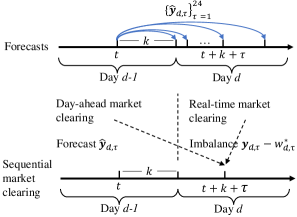
Figure 1: An illustration of the sequential market clearing.

Concretely, in the DA market, the operator determines the schedules of generators and RES to satisfy inelastic demand. The generation and RES schedule for each time-slot $\tau,\forall\tau=1,...,24$ on the next day $d$ are denoted as $\bm{p}_{d,\tau}$ and $\bm{w}_{d,\tau}$, respectively. The DA market clearing is formulated as,

$$\mathop{\min}_{\Xi_{\text{DA}}} \sum_{\tau=1}^{T}\bm{\rho}^{\top}\bm{p}_{d,\tau}$$ (1a)

s.t. $$\bm{1}^{\top}(\bm{p}_{d,\tau}+\bm{w}_{d,\tau})=\bm{1}^{\top}\bm{l}_{d,\tau},\forall\tau=1,...,T$$ (1b)

$$-\overline{\bm{f}}\leq\bm{H}(\bm{p}_{d,\tau}+\bm{w}_{d,\tau}-\bm{l}_{d,\tau})\leq\overline{\bm{f}},\forall\tau=1,...,T$$ (1c)

$$\underline{\bm{p}}\leq\bm{p}_{d,\tau}\leq\overline{\bm{p}},\forall\tau=1,...,T$$ (1d)

$$\underline{\bm{r}}\leq\bm{p}_{d,\tau}-\bm{p}_{d,\tau-1}\leq\overline{\bm{r}},\forall\tau=2,...,T$$ (1e)

$$0\leq\bm{w}_{d,\tau}\leq\hat{\bm{y}}_{d,\tau},\forall\tau=1,...,T,$$ (1f)

where $\Xi_{\text{DA}}=\{\bm{p}_{d,\tau},\bm{w}_{d,\tau}\}_{\tau=1}^{T}$. $\bm{\rho}$ is the marginal cost vector of traditional generators. RES enters the market with zero marginal cost. Each element in the vector $\bm{p}_{d,\tau}$ represents the power generated by a generator unit, whose marginal cost is in the corresponding element in $\bm{\rho}$. In the case where generators submit stepwise marginal cost curves (which is an approximation of the linear marginal cost curve [19]), the elements in $\bm{p}_{d,\tau}$ represent different generation blocks with different costs. Here, we assume there is no power loss on lines, and include a DC representation of the network. The equality constraint (1b) enforces the power balance conditions. For simplification, the demand $\bm{l}_{d,\tau}$ is considered to be known with certainty. But we note that this simplification can be easily removed. In this way, the net demand (which is demand minus RES) is uncertain and required to be forecasted. The inequality constraints (1c) restrict the scheduled power flow within the line flow limits. $\bm{H}$ in (1c) is the shift factor matrix mapping the nodal power injection to the power flow on lines [20]. (1d) and (1e) are the output power and ramping limits of the generators. (1f) limits the DA schedule of RES up to the forecast $\hat{\bm{y}}_{d,\tau}$ representing a single-value estimate of the RES production $Y_{d,\tau}$. $Y_{d,\tau}$ is a random variable, since the RES production is unknown at the moment of DA market clearing. After solving (1), the optimal solutions are obtained and denoted as $\{\bm{p}^{*}_{d,\tau},\bm{w}^{*}_{d,\tau}\}_{\tau=1}^{T}$.

Since the RES production is uncertain in DA, the DA schedules are to be adjusted at each time-slot $\tau,\forall\tau=1,...,T$ in RT on day $d$, after the RES realization $\bm{y}_{d,\tau}$ is observed. The RT market deals with the imbalance $\bm{y}_{d,\tau}-\bm{w}_{d,\tau}^{*}$ caused by RES, with a minimized imbalance cost. Additionally, the RT market clearing at time-slot $\tau,\forall\tau=2,...,T$ is influenced not only by the DA clearing outcomes but also by the extent of power adjustments made in the preceding time-slot. This is due to the ramping constraints that interconnect adjacent time slots. Because the market clearing is conducted separately for each day, the RT market clearing at time-slot $\tau=1$ on day $d$ remains unaffected by any adjustments made at time-slot $\tau=T$ on the previous day $d-1$. In the following, we firstly give the mathematical formulation of the RT clearing at $\tau=1$,

$$\mathop{\min}_{\Xi_{d,\tau}^{\text{RT}}} \ \bm{\rho}_{+}^{\top}\bm{p}_{d,\tau}^{+}-\bm{\rho}_{-}^{\top}\bm{p}^{-}_{d,\tau}$$ (2a)

s.t. $$\bm{1}^{\top}(\bm{p}_{d,\tau}^{+}-\bm{p}^{-}_{d,\tau}-\bm{\kappa}_{d,\tau})=-\bm{1}^{\top}(\bm{y}_{d,\tau}-\bm{w}^{*}_{d,\tau})$$ (2b)

$$-\overline{\bm{f}}-\bm{H}(\bm{p}_{d,\tau}^{*}+\bm{w}^{*}_{d,\tau}-\bm{l}_{d,\tau})\leq\bm{H}(\bm{p}_{d,\tau}^{+}-\bm{p}_{d,\tau}^{-}-\bm{\kappa}_{d,\tau}$$

$$\qquad+\bm{y}_{d,\tau}-\bm{w}^{*}_{d,\tau})\leq\overline{\bm{f}}-\bm{H}(\bm{p}_{d,\tau}^{*}+\bm{w}^{*}_{d,\tau}-\bm{l}_{d,\tau})$$ (2c)

$$\bm{0}\leq\bm{p}_{d,\tau}^{+}\leq\overline{\bm{p}^{+}}$$ (2d)

$$\bm{0}\leq\bm{p}_{d,\tau}^{-}\leq\overline{\bm{p}^{-}}$$ (2e)

$$\underline{\bm{p}}\leq\bm{p}_{d,\tau}^{*}+\bm{p}_{d,\tau}^{+}-\bm{p}_{d,\tau}^{-}\leq\overline{\bm{p}}$$ (2f)

$$\bm{0}\leq\bm{\kappa}_{d,\tau}\leq\bm{y}_{d,\tau}$$ (2g)

where $\Xi_{d,\tau}^{\text{RT}}=\{\bm{p}_{d,\tau}^{+},\bm{p}_{d,\tau}^{-},\bm{\kappa}_{d,\tau}\}$. The output power of generators may be increased by an amount $\bm{p}_{d,\tau}^{+}$ with the marginal cost $\bm{\rho}_{+}$ for up-regulation, or decreased by an amount $\bm{p}_{d,\tau}^{-}$ with the marginal cost $\bm{\rho}_{-}$ for down-regulation. These decisions are driven by the need to settle the RES deviation $\bm{y}_{d,\tau}-\bm{w}_{d,\tau}^{*}$ in (2b). (2c) is the power flow constraint, whose lower and upper bounds are determined by subtracting the power flow in the DA market from the line capacity. (2d) and (2e) limit the amount of up-regulation and down-regulation power to $\overline{\bm{p}^{+}},\overline{\bm{p}^{-}}$. For inflexible generators that cannot be dispatched in RT, the corresponding elements in the upper bounds will be zero, resulting in zero up- and down-adjustments for those generators. Additionally, the eventual generation power, considering the DA schedule $\bm{p}_{d,\tau}^{*}$ and the adjustment, should be within the output power limits, as stated in (2f). The inclusion of RES spill accounts for situations where the actual RES generation surpasses the scheduled amount in the DA schedule $\bm{w}_{d,\tau}^{*}$, and the excess cannot be entirely offset by the down-regulation power available from flexible generators. The amount of RES spill $\bm{\kappa}_{d,\tau}$ can be at most to its realization $\bm{y}_{d,\tau}$, as stated in (2g).

The RT clearing at time-slot $\tau,\forall\tau=2,...,T$ is,

$$\mathop{\min}_{\Xi_{d,\tau}^{\text{RT}}} \ \eqref{RTa}$$ (3a)

s.t. $$\eqref{RTb},\eqref{RTc},\eqref{RTd},\eqref{RTe},\eqref{RTf},\eqref{RTg}$$ (3b)

$$\underline{\bm{r}}\leq\bm{p}_{d,\tau}^{*}+\bm{p}_{d,\tau}^{+}-\bm{p}_{d,\tau}^{-}-$$

$$\qquad(\bm{p}_{d,\tau-1}^{*}+\bm{p}_{d,\tau-1}^{+*}-\bm{p}_{d,\tau-1}^{-*})\leq\overline{\bm{r}}$$ (3c)

The difference between the eventual generation at time-slot $\tau-1$, denoted by $\bm{p}_{d,\tau-1}^{*}+\bm{p}_{d,\tau-1}^{+*}-\bm{p}_{d,\tau-1}^{-*}$, and the eventual generation at time-slot $\tau$ must satisfy the ramping constraints, as stated in (3c).

To obtain the unique primal and dual solutions from DA and RT clearing, we require each element in the marginal cost vectors $\bm{\rho},\bm{\rho}_{+},\bm{\rho}_{-}$ are different. After solving the DA and RT market clearing, the eventual generation of the generators is either $\bm{p}_{d,\tau}^{*}+\bm{p}_{d,\tau}^{+*}$ when the RES falls short of its scheduled production in RT, or $\bm{p}_{d,\tau}^{*}-\bm{p}_{d,\tau}^{-*}$ when the RES generates more power than the schedule. Here, we define overall generation cost or the negative social surplus in a day.

Definition 1.

We define overall generation cost in a day $d$ as,

$$\sum_{\tau=1}^{T}\bm{\rho}^{\top}\bm{p}^{*}_{d,\tau}+\bm{\rho}_{+}^{\top}\bm{p}^{+*}_{d,\tau}-\bm{\rho}_{-}^{\top}\bm{p}^{-*}_{d,\tau}$$ (4a)

$$= \sum_{\tau=1}^{T}\bm{\rho}^{\top}(\bm{p}^{*}_{d,\tau}+\bm{p}^{+*}_{d,\tau})+(\bm{\rho}_{+}-\bm{\rho})^{\top}\bm{p}^{+*}_{d,\tau}+$$

$$\sum_{\tau=1}^{T}\bm{\rho}^{\top}(\bm{p}^{*}_{d,\tau}-\bm{p}^{-*}_{d,\tau})+(\bm{\rho}-\bm{\rho}_{-})^{\top}\bm{p}^{-*}_{d,\tau}$$ (4b)

$\bm{\rho}_{+}-\bm{\rho}$ and $\bm{\rho}-\bm{\rho}_{-}$ are the incremental bidding price, which reflects the marginal opportunity loss for up- and down-regulation [5]. We require them to be positive. In this way, the overall generation cost is the minimum if the generators can be dispatched to the eventual schedule in DA. Any RT adjustment would bring the extra cost either $(\bm{\rho}_{+}-\bm{\rho})^{\top}\bm{p}^{+*}_{d,\tau}$ or $(\bm{\rho}-\bm{\rho}_{-})^{\top}\bm{p}^{-*}_{d,\tau}$. The incremental bidding prices of supplying upward and downward balancing power are usually different. This explains why forecasting the expectation hardly works well in reducing the overall cost, as it overlooks the typical asymmetry affecting the RT cost.

II-B Mathematical Reformulation

In this subsection, we first convert the RT clearing in (2) and (3) into a mathematically equivalent form, and then give the compact form of DA and RT market clearing.

We reformulate the RT clearing in (2). To show the upper and lower bounds of the power adjustment more clearly, we divide the constraint (2f) into two parts. Concretely, when the RES produces less power than the schedule, we have $\bm{p}_{d,\tau}^{+}\geq\bm{0},\bm{p}_{d,\tau}^{-}=\bm{0}$. Conversely, when the RES produces more power than the schedule, we have $\bm{p}_{d,\tau}^{-}\geq\bm{0},\bm{p}_{d,\tau}^{+}=\bm{0}$. We divide (2f) into the following two constraints by the two cases,

$$\underline{\bm{p}}-\bm{p}_{d,\tau}^{*}\leq\bm{p}_{d,\tau}^{+}\leq\overline{\bm{p}}-\bm{p}_{d,\tau}^{*}$$ (5a)

$$\bm{p}_{d,\tau}^{*}-\overline{\bm{p}}\leq\bm{p}_{d,\tau}^{-}\leq\bm{p}_{d,\tau}^{*}-\underline{\bm{p}}$$ (5b)

Since $\underline{\bm{p}}\leq\bm{p}_{d,\tau}^{*}\leq\overline{\bm{p}}$, the left side of (5) is less than 0. Considering the power adjustment $\bm{p}_{d,\tau}^{+},\bm{p}_{d,\tau}^{-}$ is larger than 0 as stated in (2d) and (2e), (5) can be further simplified as,

$$\bm{0}\leq\bm{p}_{d,\tau}^{+}\leq\overline{\bm{p}}-\bm{p}_{d,\tau}^{*}$$ (6a)

$$\bm{0}\leq\bm{p}_{d,\tau}^{-}\leq\bm{p}_{d,\tau}^{*}-\underline{\bm{p}}$$ (6b)

The RT market clearing at time $\tau=1$ becomes,

$$\mathop{\min}_{\Xi_{d,\tau}^{\text{RT}}} \ \eqref{RTa}$$ (7a)

s.t. $$\eqref{RTb},\eqref{RTc},\eqref{RTd},\eqref{RTe},\eqref{reformuRT1simp},\eqref{RTg}$$ (7b)

Likewise, (3c) can be equivalently reformulated as,

$$\bm{0}\leq\bm{p}_{d,\tau}^{+}\leq\overline{\bm{r}}+(\bm{p}_{d,\tau-1}^{*}+\bm{p}_{d,\tau-1}^{+*}-\bm{p}_{d,\tau-1}^{-*})-\bm{p}_{d,\tau}^{*}$$ (8a)

$$\bm{0}\leq\bm{p}_{d,\tau}^{-}\leq\bm{p}_{d,\tau}^{*}-(\bm{p}_{d,\tau-1}^{*}+\bm{p}_{d,\tau-1}^{+*}-\bm{p}_{d,\tau-1}^{-*})-\overline{\bm{r}}$$ (8b)

The RT market clearing at time $\tau=2,...,T$ becomes,

$$\mathop{\min}_{\Xi_{d,\tau}^{\text{RT}}} \ \eqref{RTa}$$ (9a)

s.t. $$\eqref{RTb},\eqref{RTc},\eqref{RTd},\eqref{RTe},\eqref{reformuRT1simp},\eqref{reformuRT2simp},\eqref{RTg}$$ (9b)

Next, we convert the DA market clearing in (1) and the RT market clearing in (7) and (9), which are linear programs, into equivalent compact forms, with the dual variable listed after the colon. Concretely, the compact DA market clearing is,

$$\bm{x}_{d}^{*}= \mathop{\arg\min}_{\bm{x}_{d}} \quad\bm{\rho}_{\text{DA}}^{\top}\bm{x}_{d}$$ (10a)

s.t. $$\quad\bm{G}_{\text{DA}}\bm{x}_{d}\leq\bm{\psi}_{\text{DA},d}+\bm{F}_{\text{DA}}^{y}\hat{\bm{y}}_{d}:\bm{\sigma}_{d}.$$ (10b)

where $\bm{x}_{d}=[\bm{x}_{d,\tau}]_{\tau=1}^{T}=[\bm{p}_{d,\tau};\bm{w}_{d,\tau}]_{\tau=1}^{T}$ is the collection of DA decision variables. Its optimal solution is denoted as $\bm{x}_{d}^{*}=[\bm{x}_{d,\tau}^{*}]_{\tau=1}^{T}=[\bm{p}_{d,\tau}^{*};\bm{w}_{d,\tau}^{*}]_{\tau=1}^{T}$. The coefficients $\bm{\rho}_{\text{DA}},\bm{G}_{\text{DA}},\bm{\psi}_{\text{DA},d},\bm{F}_{\text{DA}}^{y}$ are constant, whose specific forms are provided in Appendix A. The RES forecasts and the demand are summarized into vectors $\hat{\bm{y}}_{d}=[\hat{\bm{y}}_{d,\tau}]_{\tau=1}^{T}$ and $\bm{l}_{d}=[\bm{l}_{d,\tau}]_{\tau=1}^{T}$, respectively. The value of $\bm{\psi}_{\text{DA},d}$ varies from day to day due to its dependence on the demand $\bm{l}_{d}$. Likewise, the RT market clearing in (7) and (9) are converted into the compact forms,

$$\bm{z}_{d,\tau}^{*}= \mathop{\arg\min}_{\bm{z}_{d,\tau}} \quad\bm{\rho}_{\text{RT}}^{\top}\bm{z}_{d,\tau}$$ (11a)

s.t. $$\quad\bm{G}_{\text{RT}}\bm{z}_{d,\tau}\leq\bm{\psi}_{\text{RT},d,\tau}+\bm{F}_{\text{RT}}\bm{x}_{d,\tau}^{*}:$$

$$\quad\bm{\nu}_{d,\tau},\forall\tau=1.$$ (11b)

$$\bm{z}_{d,\tau}^{*}= \mathop{\arg\min}_{\bm{z}_{d,\tau}} \quad\bm{\rho}_{\text{RT}}^{\top}\bm{z}_{d,\tau}$$ (12a)

s.t. $$\quad\bm{G}_{\text{RT}}^{\prime}\bm{z}_{d,\tau}\leq\bm{\psi}_{\text{RT},d,\tau}^{\prime}+[\bm{F}_{\text{RT}}^{\prime x},\bm{F}_{\text{RT}}^{\prime p},\bm{F}_{\text{RT}}^{\prime+-}]$$

$$[\bm{x}^{*}_{d,\tau},\bm{p}^{*}_{d,\tau-1},\bm{p}^{+-*}_{d,\tau-1}]^{\top}:\bm{\zeta}_{d,\tau},\forall\tau=2,...,T.$$ (12b)

where $\bm{z}_{d,\tau}=[\bm{p}_{d,\tau}^{+};\bm{p}_{d,\tau}^{-};\bm{\kappa}_{d,\tau}]$ is the collection of RT decision variables. The coefficients $\bm{\rho}_{\text{RT}},\bm{G}_{\text{RT}},\bm{\psi}_{\text{RT},d,\tau},\bm{F}_{\text{RT}}$ and $\bm{G}^{\prime}_{\text{RT}},\bm{\psi}^{\prime}_{\text{RT},d,\tau},\bm{F}^{\prime x}_{\text{RT}},\bm{F}^{\prime p}_{\text{RT}},\bm{F}^{\prime+-}_{\text{RT}}$ are constant and provided in the Appendix A. The values of $\bm{\psi}_{\text{RT},d,\tau},\bm{\psi}_{\text{RT},d,\tau}^{\prime}$ vary from hour to hour due to the dependence on the RES realization $\bm{y}_{d,\tau}$. The parameter $\bm{p}^{+-*}_{d,\tau-1}=[\bm{p}^{+*}_{d,\tau-1};\bm{p}^{-*}_{d,\tau-1}]$ is the collection of RT power adjustment for up- and down- regulation at previous time $\tau-1$.

III Methodology: Parameter Estimation

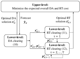
Figure 2: An illustration of the bilevel program.

In this section, a bilevel program [18] is formulated for estimating the forecast model parameter at the training phase. Let $g(\ \cdot\ ;\Theta)$ denote the forecast model with the parameter $\Theta$, and $\bm{s}_{d,\tau}$ denote the context. The RES forecast for the time-slot $\tau$ on day $d$ is issued by,

$$\hat{\bm{y}}_{d,\tau}=g(\bm{s}_{d,\tau};\Theta)$$ (13)

where $\hat{\bm{y}}_{d,\tau}$ denotes the forecast at the training phase, with $\Theta$ given by any value. Data in the training set $\{\{\bm{s}_{d,\tau},y_{d,\tau}\}_{\tau=1}^{T}\}_{d=1}^{D}$ is available, which is consisted of historical context and RES realization in $D$ days. An illustration of the bilevel program is shown in Fig. 2. The upper level determines the model parameter $\Theta$, while the lower level involves the DA and RT market clearings. The bilevel program is mathematically formulated as,

$$\underset{{\Theta}}{\mathop{\min}} \frac{1}{D\cdot T}\sum_{d=1}^{D}\{\bm{\rho}_{\text{DA}}^{\top}\bm{x}_{d}^{*}+\sum_{\tau=1}^{T}\bm{\rho}_{\text{RT}}^{\top}\bm{z}_{d,\tau}^{*}\}$$ (14a)

s.t. $$\hat{\bm{y}}_{d,\tau}=g(\bm{s}_{d,\tau};\Theta),\forall\tau=1,...,T,\forall d=1,...,D$$ (14b)

$$0\leq\hat{\bm{y}}_{d,\tau}\leq\bar{\bm{y}}_{d,\tau},\forall\tau=1,...,T,\forall d=1,...,D$$ (14c)

$$\begin{rcases}\eqref{DAcompact},\forall d=1,...,D\\ \eqref{RTcompact},\forall\tau=1,\forall d=1,...,D\\ \eqref{RTcompact2},\forall\tau=2,...,T,\forall d=1,...,D\end{rcases}\text{Lower level}$$ (14d)

where the upper-level objective (14a) seeks to minimize the expected overall operation cost of the two markets. This is achieved by leveraging the optimal DA and RT cost functions, which are informed by the decisions obtained from the lower level (14d). (14c) limits the forecast $\hat{\bm{y}}_{d,\tau}$ within $\bar{\bm{y}}_{d,\tau}$, which can be RES capacity or its offering quantity. The lower level treats the forecast $\hat{\bm{y}}_{d,\tau}$ as an input parameter. As a consequence, both DA and RT decisions are affected by it.

To show the impact of the forecast on the operation cost more clearly, we replace the lower level with the dual problems. The overall operation cost within the upper-level objective is then substituted with the DA and RT dual objectives. These objectives are constructed as a linear combination of the right-side parameters and the associated dual variables, i.e,

$$\underset{{\Theta}}{\mathop{\min}} \frac{1}{D\cdot T}\sum_{d=1}^{D}\{-\bm{\sigma}_{d}^{*\top}(\bm{\psi}_{\text{DA},d}+\bm{F}_{\text{DA}}^{y}\hat{\bm{y}}_{d})$$

$$-\bm{\nu}_{d,1}^{*\top}(\bm{\psi}_{\text{RT},d,1}+\bm{F}_{\text{RT}}\bm{x}_{d,1}^{*})+$$

$$\sum_{\tau=2}^{T}-\bm{\zeta}_{d,\tau}^{*\top}(\bm{\psi}_{\text{RT},d,\tau}^{\prime}+\bm{F}_{\text{RT}}^{\prime x}\bm{x}_{d,\tau}^{*}+\bm{F}_{\text{RT}}^{\prime p}\bm{p}_{d,\tau-1}^{*}+$$

$$\bm{F}_{\text{RT}}^{\prime+-}\bm{p}_{d,\tau-1}^{+-*})\}$$ (15a)

s.t. $$\hat{\bm{y}}_{d,\tau}=g(\bm{s}_{d,\tau};\Theta),\forall\tau=1,...,T,\forall d=1,...,D$$ (15b)

$$0\leq\hat{\bm{y}}_{d,\tau}\leq\bar{\bm{y}}_{d,\tau},\forall\tau=1,...,T,\forall d=1,...,D$$ (15c)

$$\bm{\sigma}_{d}^{*}=\mathop{\arg\max}_{\bm{\sigma}_{d}\geq 0}-\bm{\sigma}_{d}^{\top}(\bm{\psi}_{\text{DA},d}+\bm{F}_{\text{DA}}^{y}\hat{\bm{y}}_{d}),\forall d=1,...,D$$ (15d)

$$\eqref{DAcompact},\forall d=1,...,D$$ (15e)

$$\bm{\nu}_{d,1}^{*}=\mathop{\arg\max}_{\nu_{d,1}\geq 0}-\bm{\nu}_{d,1}^{\top}(\bm{\psi}_{\text{RT},d,1}+\bm{F}_{\text{RT}}\bm{x}_{d,1}^{*}),$$

$$\forall\tau=1,\forall d=1,...,D$$ (15f)

$$\eqref{RTcompact},\forall\tau=1,\forall d=1,...,D$$ (15g)

$$\bm{\zeta}_{d,\tau}^{*}=\mathop{\arg\max}_{\bm{\zeta}_{d,\tau}\geq 0}-\bm{\zeta}_{d,\tau}^{\top}(\bm{\psi}_{\text{RT},d,\tau}^{\prime}+\bm{F}_{\text{RT}}^{\prime x}\bm{x}_{d,\tau}^{*}+\bm{F}_{\text{RT}}^{\prime p}\bm{p}_{d,\tau-1}^{*}+$$

$$\bm{F}_{\text{RT}}^{\prime+-}\bm{p}_{d,\tau-1}^{+-*}),\forall\tau=2,...,T,\forall d=1,...,D$$ (15h)

$$\eqref{RTcompact2},\forall\tau=2,...,T-1,\forall d=1,...,D$$ (15i)

Since RT clearing requires the primal solutions of DA clearing and the previous RT clearing as input parameters, we also include the primal problems in the lower level. The forecast $\hat{\bm{y}}_{d}$ affects the upper-level objective (15a) via its impact on the DA and RT dual solutions $\bm{\sigma}_{d}^{*},\bm{\nu}_{d,1}^{*},\bm{\zeta}_{d,\tau}^{*}$, and their primal solutions $\bm{x}^{*}_{d,\tau},\bm{p}^{*}_{d,\tau-1},\bm{p}^{+-*}_{d,\tau-1}$. If we can obtain the function between them and the forecast $\hat{\bm{y}}_{d}$ directly, the upper-level objective can be rewritten as a function regarding the forecast $\hat{\bm{y}}_{d}$, and can be used as the loss function for training. In the next section, we will show how to achieve this.

At the operation phase, the forecast $\bm{\hat{y}}_{d,\tau}$ under the context $\bm{s}_{d,\tau}$ can be obtained by the trained model. Subsequently, utilizing this forecast, the operator proceeds to solve the DA market clearing in (1), followed by the RT market clearing in (2) and (3).

IV Loss Function Design

We derive the loss function based on the bilevel program in (15). We first analyze how forecasts influence the DA and RT optimal solutions. Based on it, a loss function is derived, and will be used for training a forecast model.

IV-A The Impact of the Forecast on the DA and RT Solutions

This section analyzes the impact of the forecasts on the primal and dual solutions of DA and RT market clearings. Specifically, we derive analytical functions that quantitatively depict the impact of the forecasts on the optimal primal and dual solutions. As a parameter to the DA market clearing (10), forecasts $\hat{\bm{y}}_{d}$ influence DA primal and dual solutions directly. As for the RT market clearing, the impact of the forecast is indirect, as it does not directly appear as the parameter in (11) or (12). Concretely, for the RT market clearing at time-slot $\tau=1$, the forecast $\hat{\bm{y}}_{d}$ influences $\bm{x}_{d,1}^{*}$, and then $\bm{x}_{d,1}^{*}$ influences the RT solutions, with the first impact being determined by the DA clearing (10), and the second impact by the RT clearing (11). For the RT clearing at time-slot $\tau=2,...,T$, the impact of the forecast is complex. The forecast $\hat{\bm{y}}_{d}$ affects the DA solutions $\bm{x}_{d,\tau}^{*},\bm{p}_{d,\tau-1}^{*}$ through the DA clearing (10). Its influence on the RT solutions $\bm{p}_{d,\tau-1}^{+-*}$ at the previous time-slot $\tau-1$ occurs as explained earlier. Then, the influence of the parameters $\bm{x}_{d,\tau}^{*},\bm{p}^{*}_{d,\tau-1},\bm{p}^{+-*}_{d,\tau-1}$ on the RT clearing solutions at time $\tau$ is determined by (12). The above process is summarized in Fig. 3.

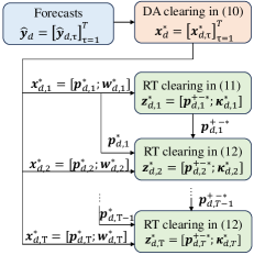
Figure 3: An illustration of the impact of forecasts on DA and RT primal solutions.

Since the core of the above analysis is understanding the impact of the parameters on the optimization solutions, we use the multiparametric theory for this end. A general linear program (16) is used as an example. We firstly define primal and dual decision policies. Then, the theorem regarding them is presented.

$$\bm{x}^{*}= \mathop{\arg\min}_{\bm{x}} \quad\bm{c}^{\top}\bm{x}$$ (16a)

s.t. $$\quad\bm{G}\bm{x}\leq\bm{\psi}+\bm{F}\bm{\omega}:\bm{\sigma}.$$ (16b)

Definition 2.

(Primal and dual decision policies) Primal and dual decision policies are functions defined across the polyhedral set $\Omega$, which describe the change in the optimal primal and dual solutions, i.e., $\bm{x}^{*}$ and $\bm{\sigma}^{*}$, as the parameter $\bm{\omega}$ varies in $\Omega$.

Theorem 1.

[21] Consider the linear program (16) and the parameter $\bm{\omega}\in\Omega$. The primal and dual decision policies are a piecewise linear function and a stepwise function respectively, if there exists a polyhedral partition $R_{1},...,R_{N}$ of $\Omega$, and $\forall\bm{\omega}\in R_{i}$, the primal decision policy is linear, and the dual decision policy is a constant function.

Theorem 1 implies that in a neighborhood of the parameter, the primal decision policy is represented by a linear function, whereas the corresponding dual decision policy remains a constant function. Given a specific value of $\bm{w}$, we study the local policies defined in its neighborhood. The local dual decision policy can be obtained easily, as it is a constant function. Its output is the optimal dual solution obtained by solving the dual problem of (16), given the value of $\bm{\omega}$. Additionally, after solving (16), the active constraints of (16b) can be obtained. Let $\mathcal{J}$ denote the row index set associated with (16b), and $\mathcal{J}^{a}$ denote the row index set of the active constraints. The parameters associated with the active constraints are denoted as $\bm{G}_{\mathcal{J}^{a}},\bm{\psi}_{\mathcal{J}^{a}},\bm{F}_{\mathcal{J}^{a}}$. They are the sub-matrices and sub-vectors of $\bm{G},\bm{\psi},\bm{F}$ and are comprised by the rows of $\bm{G},\bm{\psi},\bm{F}$ in the row index sets $\mathcal{J}^{a}$. We have the following proposition for the local primal decision policy,

Proposition 1.

The local primal decision policy of (16) is,

$$\bm{x}^{*}=\bm{G}_{\mathcal{J}^{a}}^{-1}(\bm{\psi}_{\mathcal{J}^{a}}+\bm{F}_{\mathcal{J}^{a}}\bm{\omega})$$ (17)

Proof.

With the active constraints of (16), we have $\bm{G}_{\mathcal{J}^{a}}\bm{x}^{*}=\bm{\psi}_{\mathcal{J}^{a}}+\bm{F}_{\mathcal{J}^{a}}\bm{\omega}$. $\bm{G}_{\mathcal{J}^{a}}^{-1}$ is the pseudo inverse of $\bm{G}_{\mathcal{J}^{a}}$. By moving $\bm{G}_{\mathcal{J}^{a}}$ from left to right, we have (17). ∎

Remark 1.

(17) calculates the inverse of $\bm{G}_{\mathcal{J}^{a}}$, whose computational complexity depends on the matrix size, i.e., $|\mathcal{J}^{a}|$. We note that a similar matrix inverse is also involved in [15], with the matrix size of $|\mathcal{J}|+\iota$, where $\iota$ is the dimension of $\bm{x}$. There is $|\mathcal{J}|+\iota>|\mathcal{J}^{a}|$. Therefore, the computation burden of [15] is larger.

With Proposition 1, we present the local primal decision policy for the DA clearing (10), and RT clearing (11) and (12). Let $\mathcal{J}^{a}_{\text{DA},d},\mathcal{J}^{a}_{\text{RT},d,\tau},\forall\tau=1,...,T$ denote the row index set of active constraints (10b), (11b), and (12b). The parameters associated with the active constraints are denoted as $\bm{G}_{\text{DA},\mathcal{J}_{\text{DA},d}^{a}},\bm{\psi}_{\text{DA},d,\mathcal{J}_{\text{DA},d}^{a}},\bm{F}_{\text{DA},\mathcal{J}_{\text{DA},d}^{a}}^{y}$, $\bm{G}_{\text{RT},\mathcal{J}_{\text{RT},d,\tau}^{a}},\bm{\psi}_{\text{RT},d,\tau,\mathcal{J}_{\text{RT},d,\tau}^{a}},\bm{F}_{\text{RT},\mathcal{J}_{\text{RT},d,\tau}^{a}}$, and $\bm{G}_{\text{RT},\mathcal{J}_{\text{RT},d,\tau}^{a}}^{\prime},\bm{\psi}_{\text{RT},d,\tau,\mathcal{J}_{\text{RT},d,\tau}^{a}}^{\prime},\bm{F}_{\text{RT},\mathcal{J}_{\text{RT},d,\tau}^{a}}^{\prime x},\bm{F}_{\text{RT},\mathcal{J}_{\text{RT},d,\tau}^{a}}^{\prime p},\bm{F}_{\text{RT},\mathcal{J}_{\text{RT},d,\tau}^{a}}^{\prime+-}$, respectively. We have the following proposition for the local primal decision policies of (10), (11), and (12).

Proposition 2.

The local primal decision policies of (10),(11) and (12) are,

$$\bm{x}_{d}^{*}=\bm{G}_{\text{DA},\mathcal{J}_{\text{DA},d}^{a}}^{-1}(\bm{\psi}_{\text{DA},d,\mathcal{J}_{\text{DA},d}^{a}}+\bm{F}_{\text{DA},\mathcal{J}_{\text{DA},d}^{a}}^{y}\hat{\bm{y}}_{d})$$ (18)

$$\bm{z}_{d,\tau}^{*}=\bm{G}_{\text{RT},\mathcal{J}_{\text{RT},d,\tau}^{a}}^{-1}(\bm{\psi}_{\text{RT},d,\tau,\mathcal{J}_{\text{RT},d,\tau}^{a}}+\bm{F}_{\text{RT},\mathcal{J}^{a}_{\text{RT},d,\tau}}\bm{x}_{d,\tau}^{*}),\forall\tau=1$$ (19)

$$\begin{split}&\bm{z}_{d,\tau}^{*}=\bm{G}_{\text{RT},\mathcal{J}_{\text{RT},d,\tau}^{a}}^{\prime-1}(\bm{\psi}^{\prime}_{\text{RT},d,\tau,\mathcal{J}_{\text{RT},d,\tau}^{a}}+\bm{F}_{\text{RT},\mathcal{J}_{\text{RT},d,\tau}^{a}}^{\prime x}\bm{x}_{d,\tau}^{*}+\\ &\bm{F}_{\text{RT},\mathcal{J}_{\text{RT},d,\tau}^{a}}^{\prime p}\bm{p}_{d,\tau-1}^{*}+\bm{F}_{\text{RT},\mathcal{J}_{\text{RT},d,\tau}^{a}}^{\prime+-}\bm{p}_{d,\tau-1}^{+-*}),\forall\tau=2,...,T\end{split}$$ (20)

Eq. (18) is a linear function of $\hat{\bm{y}}_{d}$, whose output is the DA solution $\bm{x}_{d}^{*}$ on the day $d$. In the following, we show how to rewrite (19) and (20) as a function of the forecast $\hat{\bm{y}}_{d}$.

In addition, we define an operator $\Pi_{\mathcal{J}}:h(\bm{x})\mapsto\tilde{h}(\bm{x})$, where $h(\bm{x})=\bm{A}\bm{x}+\bm{b}$ is a linear function with the parameter $\bm{A},\bm{b}$, and $\mathcal{J}$ is the row index subset of $\bm{A},\bm{b}$. The output $\tilde{h}(\bm{x})$ of the operator is also a linear function, where $\tilde{h}(\bm{x})=\bm{A}_{\mathcal{J}}\bm{x}+\bm{b}_{\mathcal{J}}$ and $\bm{A}_{\mathcal{J}},\bm{b}_{\mathcal{J}}$ are the sub-matrix and sub-vector of $\bm{A},\bm{b}$.

Let $\mathcal{I}_{\text{DA},d,\tau}$ denote the row index set corresponding to $\bm{x}_{d,\tau}^{*}$ within $\bm{x}_{d}^{*}$. The function that maps $\hat{\bm{y}}_{d}$ to $\bm{x}_{d,\tau}^{*}$ is,

$$\begin{split}&f^{x}_{d,\tau}(\hat{\bm{y}}_{d}):=\bm{x}_{d,\tau}^{*}=\Pi_{\mathcal{I}_{\text{DA},d,\tau}}(\bm{G}_{\text{DA},\mathcal{J}_{\text{DA},d}^{a}}^{-1}\bm{F}_{\text{DA},\mathcal{J}_{\text{DA},d}^{a}}^{y}\hat{\bm{y}}_{d}+\\ &\bm{G}_{\text{DA},\mathcal{J}_{\text{DA},d}^{a}}^{-1}\bm{\psi}_{\text{DA},d,\mathcal{J}_{\text{DA},d}^{a}}),\forall\tau=1,...,T\end{split}$$ (21)

The coefficients are determined by the coefficients of (18), whose row indexes belong to the set $\mathcal{I}_{\text{DA},d,\tau}$. By substituting (21) into (19), we can obtain the function between RT primal solution $\bm{z}_{d,\tau}^{*}$ at time-slot $\tau=1$ and the forecast $\hat{\bm{y}}_{d}$.

$$\begin{split}&f_{d,\tau}^{z}(\hat{\bm{y}}_{d}):=\bm{z}_{d,\tau}^{*}=\bm{G}_{\text{RT},\mathcal{J}_{\text{RT},d,\tau}^{a}}^{-1}\bm{F}_{\text{RT},\mathcal{J}^{a}_{\text{RT},d,\tau}}f_{d,\tau}^{x}(\hat{\bm{y}}_{d})+\\ &\bm{G}_{\text{RT},\mathcal{J}_{\text{RT},d,\tau}^{a}}^{-1}\bm{\psi}_{\text{RT},d,\tau,\mathcal{J}_{\text{RT},d,\tau}^{a}},\forall\tau=1\end{split}$$ (22)

To obtain the function between RT primal solution $\bm{z}_{d,\tau}^{*}$ at time-slot $\tau=2,...,T$ and the forecast $\hat{\bm{y}}_{d}$, we need to obtain the function between DA solution $\bm{p}_{d,\tau-1}^{*}$, RT solution $\bm{p}_{d,\tau-1}^{+-*}$ and the forecast $\hat{\bm{y}}_{d}$ as well. Concretely, since $\bm{p}_{d,\tau-1}^{*}$ is a part of $\bm{x}_{d,\tau-1}^{*}$, let $\mathcal{I}_{\text{DA},d,\tau-1}^{p}$ be the row index set corresponds to $\bm{p}_{d,\tau-1}^{*}$ within $\bm{x}_{d,\tau-1}^{*}$. With (21), the function between $\bm{p}_{d,\tau-1}^{*}$ and the forecast $\hat{\bm{y}}_{d}$ is,

$$\begin{split}&f^{p}_{d,\tau-1}(\hat{\bm{y}}_{d}):=\bm{p}_{d,\tau-1}^{*}=\Pi_{\mathcal{I}_{\text{DA},d,\tau-1}^{p}}(f_{d,\tau-1}^{x}(\hat{\bm{y}}_{d})),\\ &\forall\tau=2,...,T\end{split}$$ (23)

Likewise, since $\bm{p}_{d,\tau-1}^{+-*}$ is a part of $\bm{z}_{d,\tau-1}^{*}$, let $\mathcal{I}_{\text{RT},d,\tau-1}^{+-}$ be the row index set corresponds to $\bm{p}_{d,\tau-1}^{+-*}$ within $\bm{z}_{d,\tau-1}^{*}$. We can express a function of $\bm{p}_{d,\tau-1}^{+-*}$ w.r.t. $\hat{\bm{y}}_{d}$ as,

$$\begin{split}&f_{d,\tau-1}^{+-}(\hat{\bm{y}}_{d}):=\bm{p}_{d,\tau-1}^{+-*}=\Pi_{\mathcal{I}_{\text{RT},d,\tau-1}^{+-}}(f_{d,\tau-1}^{z}(\hat{\bm{y}}_{d})),\\ &\forall\tau=2,...,T\end{split}$$ (24)

Accordingly, by substituting (21), (23), (24) into (20), the function between $\bm{z}_{d,\tau}^{*}$ at time-slot $\tau=2,...,T$ is,

$$\begin{split}&f^{z}_{d,\tau}(\hat{\bm{y}}_{d}):=\\ &\bm{z}_{d,\tau}^{*}=\bm{G}_{\text{RT},\mathcal{J}_{\text{RT},d,\tau}^{a}}^{\prime-1}(\bm{\psi}^{\prime}_{\text{RT},d,\tau,\mathcal{J}_{\text{RT},d,\tau}^{a}}+\bm{F}_{\text{RT},\mathcal{J}_{\text{RT},d,\tau}^{a}}^{\prime x}f_{d,\tau}^{x}(\hat{\bm{y}}_{d})+\\ &\bm{F}_{\text{RT},\mathcal{J}_{\text{RT},d,\tau}^{a}}^{\prime p}f_{d,\tau-1}^{p}(\hat{\bm{y}}_{d})+\bm{F}_{\text{RT},\mathcal{J}_{\text{RT},d,\tau}^{a}}^{\prime+-}f_{d,\tau-1}^{+-}(\hat{\bm{y}}_{d})),\\ &\forall\tau=2,...,T\end{split}$$ (25)

To sum up, the function between the forecast $\hat{\bm{y}}_{d}$ and DA and RT primal solutions, which is defined in the neighborhood of $\hat{\bm{y}}_{d}$, are summarized in the (21)-(25). The function between the optimal dual solutions and the forecast $\hat{\bm{y}}_{d}$ is a constant function, whose output can be obtained by solving the dual problems of (10),(11), and (12). With these, we are ready to transform the upper-level objective (15a) to a function of the forecast $\hat{\bm{y}}_{d}$. The details are in the next subsection.

IV-B Loss Function Derivation

In this subsection, we derive the loss function in the neighborhood of the forecast $\hat{\bm{y}}_{d}$. By substituting the functions (21),(23),(24) and dual solutions into the upper-level objective (15a), the loss function in the neighborhood of the forecast $\hat{\bm{y}}_{d}$ is,

$$\ell_{d}(\hat{\bm{y}}_{d}):=-\bm{\sigma}_{d}^{*\top}(\bm{\psi}_{\text{DA},d}+\bm{F}_{\text{DA}}^{y}\hat{\bm{y}}_{d})-\bm{\nu}_{d,1}^{*\top}(\bm{\psi}_{\text{RT},d,1}+$$

$$\bm{F}_{\text{RT}}f_{d,1}^{x}(\hat{\bm{y}}_{d}))+\sum_{\tau=2}^{T}-\bm{\zeta}_{d,\tau}^{*\top}(\bm{\psi}_{\text{RT},d,\tau}^{\prime}+\bm{F}_{\text{RT}}^{\prime x}f_{d,\tau}^{x}(\hat{\bm{y}}_{d})+$$

$$\bm{F}_{\text{RT}}^{\prime p}f_{d,\tau-1}^{p}(\hat{\bm{y}}_{d})+\bm{F}_{\text{RT}}^{\prime+-}f_{d,\tau-1}^{+-}(\hat{\bm{y}}_{d}))$$ (26a)

$$\eqref{functionxd},\eqref{functionp},\eqref{functionadj}$$ (26b)

Since functions in (26b) are linear, and the dual decision policies are constant, the loss function $\ell_{d}(\hat{\bm{y}}_{d})$ in the neighborhood of the forecast $\hat{\bm{y}}_{d}$ is linear, and output the overall operation cost (4a) given the forecast $\hat{\bm{y}}_{d}$. Naturally, the derivative of $\ell_{d}(\hat{\bm{y}}_{d})$ w.r.t. the forecast $\hat{\bm{y}}_{d}$, i.e., $\frac{\ell_{d}(\hat{\bm{y}}_{d})}{\hat{\bm{y}}_{d}}$, measures the marginal impact of the forecast on the overall cost. It is derived as,

$$\begin{split}&(\frac{\ell_{d}(\hat{\bm{y}}_{d})}{\hat{\bm{y}}_{d}})^{\top}=-\bm{\sigma}_{d}^{*\top}\bm{F}_{\text{DA}}^{y}-\bm{\nu}_{d,1}^{*\top}\bm{F}_{\text{RT}}\frac{\partial f_{d,1}^{x}(\hat{\bm{y}}_{d})}{\partial\hat{\bm{y}}_{d}}+\sum_{\tau=2}^{T}-\bm{\zeta}_{d,\tau}^{*T}\\ &(\bm{F}_{\text{RT}}^{\prime x}\frac{\partial f_{d,\tau}^{x}(\hat{\bm{y}}_{d})}{\partial\hat{\bm{y}}_{d}}+\bm{F}_{\text{RT}}^{\prime p}\frac{\partial f_{d,\tau-1}^{p}(\hat{\bm{y}}_{d})}{\partial\hat{\bm{y}}_{d}}+\bm{F}_{\text{RT}}^{\prime+-}\frac{\partial f_{d,\tau-1}^{+-}(\hat{\bm{y}}_{d})}{\partial\hat{\bm{y}}_{d}})\end{split}$$ (27)

According to Theorem 1, the loss function defined across the entire space of $\hat{\bm{y}}_{d}$ is expected to be a piecewise linear function. Specifically, each piece is related with a different active constraint index sets $\mathcal{J}^{a}_{\text{DA},d},\mathcal{J}^{a}_{\text{RT},d,\tau},\forall\tau=1,...,T$ of DA and RT market clearings. Such index sets then determine the primal decision policies (18)-(20), and the following functions in (21)-(25). It is possible to enumerate all possible active constraint index sets, and derive the corresponding loss function [22]. However, implementing such a practice can be computationally expensive, particularly when dealing with large-scale optimization problems. We notice that the derivatives $\frac{\partial f_{d,\tau}^{x}(\hat{\bm{y}}_{d})}{\partial\hat{\bm{y}}_{d}}$, $\frac{\partial f_{d,\tau-1}^{p}(\hat{\bm{y}}_{d})}{\partial\hat{\bm{y}}_{d}}$, $\frac{\partial f_{d,\tau-1}^{+-}(\hat{\bm{y}}_{d})}{\partial\hat{\bm{y}}_{d}}$ in (27) associated with the active index sets are constants, as (21),(23),(24) are linear functions. This suggests that there is no need to recalculate these derivatives when encountering the same active index sets during the training. For that, we propose a solution strategy, where the derivatives are recalculated only when encountering new ones.

V Solution Strategy

We illustrate the training phase of the forecast model based on neural networks (NNs). With the loss function, we use batch optimization to train NN. Given a batch of data in $B$ days, the parameter estimation with the derived loss function is formulated as,

$$\underset{{\Theta}}{\mathop{\min}} \frac{1}{B\cdot T}\sum_{d=1}^{B}\ell_{d}(\hat{\bm{y}}_{d})$$ (28a)

s.t. $$\hat{\bm{y}}_{d,\tau}=g(\bm{s}_{d,\tau};\Theta),\forall\tau=1,...,T,\forall d=1,...,B$$ (28b)

$$0\leq\hat{\bm{y}}_{d,\tau}\leq\bar{\bm{y}}_{d,\tau},\forall\tau=1,...,T,\forall d=1,...,B$$ (28c)

Different from the conventional unconstrained program at the training phase, (28) is with the box constraint (28c) for the NN output. We design a specific model structure to address this. Specifically, a Sigmoid function, whose output is between 0 and 1, is used as the activation function at the output layer. By multiplying its output with the cap $\bar{\bm{y}}_{d,\tau}$ of each sample, the box constraint (28c) is satisfied. NN’s structure is illustrated in Fig. 4.

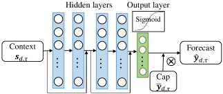
Figure 4: The structure of neural network.

During the training, the NN, with the parameter $\Theta$ given by any value, outputs the forecast $\hat{\bm{y}}_{d,\tau}$ by (13). The primal and dual problems of DA and RT clearing in (10),(11),(12) are solved. The active constraint index sets $\mathcal{J}^{a}_{\text{DA},d},\mathcal{J}^{a}_{\text{RT},d,\tau},\forall\tau=1,...,T$ and the dual solutions $\bm{\sigma}_{d}^{*},\bm{\nu}_{d,1}^{*},\bm{\zeta}_{d,\tau}^{*},\forall\tau=2,...,T$ are obtained. We check whether they are the new ones. If yes, we calculate derivatives $\frac{\partial f_{d,\tau}^{x}(\hat{\bm{y}}_{d})}{\partial\hat{\bm{y}}_{d}}$, $\frac{\partial f_{d,\tau-1}^{p}(\hat{\bm{y}}_{d})}{\partial\hat{\bm{y}}_{d}}$, $\frac{\partial f_{d,\tau-1}^{+-}(\hat{\bm{y}}_{d})}{\partial\hat{\bm{y}}_{d}}$ associated with the new ones, and calculate the gradient $\frac{\ell_{d}(\hat{\bm{y}}_{d})}{\hat{\bm{y}}_{d}}$ in (27). Additionally, we store the new active index sets and the associated derivatives in the buffers. If not, the stored elements in the buffers are used for calculating the gradient. The training process is summarized in Fig. 5.

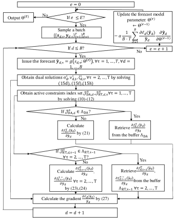
Figure 5: The flowchart of the algorithm for the training phase. Require: Learning rate $\alpha$, batch size $B$, initialized buffers $\Lambda_{\text{DA}},\Lambda_{\text{RT},\tau},\forall\tau=1,...,T$ for storing active constraint index set/derivative, and initialized forecast model parameters $\Theta^{(0)}$.

VI Case Study

We consider a modified version of IEEE 9-Bus system [23]. As shown in Fig. 6, the system consists of 3 loads, 2 wind farms, and 3 generators ($G_{1},G_{2},G_{3}$) whose generation needs to be settled in the DA market and can be adjusted for providing up- and down-regulation power in the RT market. The generators submit the marginal generation cost $\bm{\rho}$, the minimum generation power $\underline{\bm{p}}$, the maximum generation power $\overline{\bm{p}}$, the ramping limits $\underline{\bm{r}},\overline{\bm{r}}$ in the DA market, which are provided in Table I. The marginal generation cost $\bm{\rho}_{+},\bm{\rho}_{-}$ for the power adjustment, the marginal opportunity loss $\bm{\rho}_{+}-\bm{\rho},\bm{\rho}-\bm{\rho}_{-}$ and the adjustment limits $\overline{\bm{p}^{+}}$ and $\overline{\bm{p}^{-}}$, that generators submit in the RT market, are provided in Table I as well. The yearly demand consumption data is used, with a valley value of 210 MW, and a peak value of 265 MW. The hourly wind power production in the year of 2012 from GEFCom 2014 is used, whose range is from 0 to 1. The wind data is scaled by multiplying a constant according to the considered wind generation capacity, which will be discussed in the following sections. The demand and wind data can be found in [24].

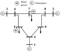
Figure 6: The illustration of IEEE 9-bus system.

Table I: Cost and technical data in DA and RT market.

		$G_{1}$	$G_{2}$	$G_{3}$
	Marginal generation cost $\bm{\rho}$ ($/MW)	20	22	24
	Minimum generation power $\underline{\bm{p}}$ (MW)	0	0	0
DA market	Maximum generation power $\overline{\bm{p}}$ (MW)	150	200	270
	Lower ramping limits $\underline{\bm{r}}$ (MW)	-90	-80	-70
	Upper ramping limits $\overline{\bm{r}}$ (MW)	90	80	70
	Marginal up-regulation cost $\bm{\rho}_{+}$ ($/MW)	50	52	54
	Marginal down-regulation cost $\bm{\rho}_{+}$ ($/MW)	18	16	14
	Marginal opportunity loss for up-regulation $\bm{\rho}_{+}-\bm{\rho}$ ($/MW)	30	30	30
RT Market	Marginal opportunity loss for down-regulation $\bm{\rho}-\bm{\rho}_{-}$ ($/MW)	2	6	10
	Up-regulation limit $\overline{\bm{p}^{+}}$ (MW)	60	60	60
	Down-regulation limit $\overline{\bm{p}^{-}}$ (MW)	60	60	60

We use a four-layer ResNet as the forecast model, which has 256 hidden layer units. Its structure is described in Figure 4. The input context consists of the numeric weather prediction (i.e., the predicted wind speed and direction at 10m and 100m altitude) of each wind farm in the system. We use Root Mean Squared Error (RMSE) on the test set for assessing the forecast quality, and the average overall operation cost on the test set, as defined in (4a), for evaluating the operation value. Four benchmark models are used for comparison: Two quality-oriented, one value-oriented forecasting approach, and a stochastic program. The two quality-oriented forecast models are trained using Mean Squared Error (MSE) and pinball loss (an asymmetric loss function), denoted as Qua-E and Qua-Q, respectively. Specifically, Qua-E provides predictions for expected wind power, while Qua-Q offers quantile predictions. Light Gradient Boosted Machine is used for issuing quantiles, which is the winner of GEFCom 2014 [25]. We consider the value-oriented forecast model trained via OptNet [15] as a benchmark, referred to as OptNet. Lastly, the stochastic program, with 50 wind power scenarios obtained by k-nearest-neighbors, is considered and denoted as Sto-OPT. For each sample on test set, the stochastic program is solved for settling the schedule of generators and wind power in DA. Then, the adjustment in (11) and (12) are performed in RT.

VI-A The Operational Advantage

The capacity of two wind farms is set as 105 MW, respectively, which takes up 79% of the maximum demand. The nominal level of Qua-Q issued quantile is chosen as $\frac{1}{16}$. Such nominal level is determined by $\frac{\bm{\rho}^{1}-\bm{\rho}_{-}^{1}}{\bm{\rho}_{+}^{1}-\bm{\rho}_{-}^{1}}$ [16], where $\bm{\rho}^{1},\bm{\rho}_{-}^{1},\bm{\rho}_{+}^{1}$ represent the marginal costs of $G_{1}$. The results of RMSE and average operation cost, along with training time per NN epoch and test time, are reported in Table II.

Since Sto-OPT does not need training or rely on a point forecast, its RMSE is not reported. Sto-OPT serves as the ideal benchmark [9], which has the least average operation cost. The proposed approach outperforms all other methods in terms of average operation cost on the test set, except for Sto-OPT. However, its test time is much shorter than Sto-OPT, demonstrating computational efficiency. Also, we observe that the performance of Sto-OPT is heavily influenced by the number of scenarios used. When fewer scenarios, such as 20, are employed, the average operation cost on the test set increases to $84,478, which is even worse than that achieved by the proposed approach.

The proposed approach exhibits a higher RMSE compared to Qua-E. This underscores the point that more accurate forecasts don’t always translate to better operational performance. Additionally, since the incremental bidding price $\bm{\rho}_{+}-\bm{\rho}$ is larger than $\bm{\rho}-\bm{\rho}_{-}$, the marginal opportunity loss of up-regulation is larger than that of down-regulation. Therefore, Qua-Q, which issues the quantile forecasts with a low proportion level ($\frac{1}{16}$), has better performance than Qua-E. As for the training time, the proposed approach requires a longer training time than Qua-E due to the more complex computation involved in calculating the gradient during the training process. But it is still acceptable, and much shorter than the value-oriented forecasting approach OptNet.

Table II: RMSE, average operation cost on the test set and the training/test time of the proposed approach and benchmarks.

	Proposed	Qua-E	Qua-Q	OptNet	Sto-OPT
RMSE (MW)	26	18	29	33	-
Average operation cost ($)	84449	86990	85154	86347	84362
Training time per epoch	25 s	0.08 s	-	136 s	-
Test time	5 s	5 s	5 s	5 s	64min

VI-B The Sensitivity Analysis

In this section, we compare the proposed approach against Qua-E under different wind power capacities and adjustment cost $\overline{\bm{\rho}^{+}}$ for up-regulation.

VI-B1 Performance under Different Wind Power Penetration

Here, different wind power capacities are considered, i.e., 85 MW, 95 MW, and 105 MW per wind farm. Fig. 7 shows the average operation cost of the proposed approach and Qua-E under different wind power capacities. Under large wind power capacity, the average cost reduction of the proposed approach is more obvious. For instance, such a reduction is 2.4% and 2.9%, respectively, under the wind power capacity of 85 MW and 105 MW. Therefore, the proposed approach has larger operation benefits under large penetration of wind power.

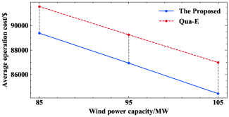
Figure 7: Average operation cost under different values of wind power capacity. Qua-E stands for quality-oriented forecast issuing expectation.

VI-B2 Performance under Different Up-regulation Cost in RT

The performance is further tested under various up-regulation costs, along with the marginal opportunity loss $\bm{\rho}_{+}-\bm{\rho}$ for up-regulation. The marginal opportunity loss $\bm{\rho}-\bm{\rho}_{-}$ for down-regulation is the same as in Table I. The capacity of wind power is set to 105 . The average operation cost of the proposed approach and Qua-E under two settings are listed in Table III. When the RT market lacks flexibility for up-regulation, the up-regulation cost is high, and the marginal opportunity loss for up-regulation is much larger than that for down-regulation. Therefore, the proposed approach tends to forecast less power than Qua-E to mitigate the risk of costly up-regulation, and results in a significant cost reduction (8%). When the up-regulation cost is similar to the DA marginal generation cost $\bm{\rho}$, the marginal opportunity loss for up-regulation is lower than that for down-regulation. Therefore, the proposed approach tends to forecast more power to mitigate the risk of costly down-regulation. In such case, since the marginal opportunity losses of up- and down-regulation is very similar, the cost reduction of the proposed approach is less significant. The forecast profiles for 6 days of wind farm at the node 5 under the two settings are given in Fig. 8.

To sum up, the operation advantage of the proposed approach is more evident, under large penetration of wind power, and high up-regulation cost.

Table III: Average operation cost in different settings of up-regulation costs in RT. The first column gives the RT up-regulation costs and marginal opportunity loss in each setting. Inside the parenthesis, the up-regulation costs are given on the left of the slash, and the marginal opportunity loss is given on the right.

Settings	Proposed ($)	Qua-E ($)	Cost reduction (%)
High up- regulation cost ($G_{1}$: 80/60, $G_{2}$: 82/60, $G_{3}$: 84/60)	85114	92486	8%
Low up- regulation cost ($G_{1}$: 21/1, $G_{2}$: 23/1, $G_{3}$: 25/1)	81517	81677	0.2%

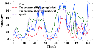
Figure 8: The 6-day wind power forecast profiles for a wind farm connected to Node 5 are provided by Qua-E and the proposed approach under both high and low up-regulation cost settings.

VII Conclusions

We propose a value-oriented renewable energy forecasting approach, for minimizing the expected overall operation cost in the existing deterministic market clearing framework. We analytically derive the loss function for value-oriented renewable energy forecasting in sequential market clearing. The loss function is proved to be piecewise linear when the market clearing is modeled by linear programs. Additionally, we provide the analytical gradient of the loss function with respect to the forecast, which leads to an efficient training strategy. In the case study, compared to quality-oriented forecasting approach trained by MSE, the proposed approach can reduce average operation cost on the test set to 2.9%. Such an advantage is more obvious under large wind power capacity and high up-regulation costs. Under high up-regulation costs, our approach can reduce the cost by up to 8%. Future work will include attempts to derive the loss function for market clearing modeled by other types of optimization programs, such as quadratic optimization or conic optimization.

Appendix A Details of Coefficients in Day-Ahead and Real-Time Clearings

We first provide the details of coefficients in DA clearing (10). For that, we turn each constraint in (1) into the compact form. Let $\tilde{\bm{H}}=[\bm{H},\bm{H}]$ denote the horizontal stack of the matrix $\bm{H}$, $\tilde{\bm{E}}=[\bm{E},\bm{O}]$, $\hat{\bm{E}}=[\bm{O},\bm{E}]$ be the stack of an identity matrix and an all-zero matrix. Next, we define the following matrices, which are used for forming the coefficients in (10),

$$\bm{D}_{1}=\begin{bmatrix}\bm{1}^{\top}&\bm{0}^{\top}&\dots&\bm{0}^{\top}\\ \bm{0}^{\top}&\bm{1}^{\top}&\dots&\bm{0}^{\top}\\ \vdots&\vdots&\ddots\\ \bm{0}^{\top}&\bm{0}^{\top}&\dots&\bm{1}^{\top}\end{bmatrix}\bm{D}_{2}=\begin{bmatrix}\tilde{\bm{H}}&\bm{O}&\dots&\bm{O}\\ \bm{O}&\tilde{\bm{H}}&\dots&\bm{O}\\ \vdots&\vdots&\ddots\\ \bm{O}&\bm{O}&\dots&\tilde{\bm{H}}\end{bmatrix}$$

$$\bm{D}_{3}=\begin{bmatrix}\tilde{\bm{E}}&\bm{O}&\dots&\bm{O}\\ \bm{O}&\tilde{\bm{E}}&\dots&\bm{O}\\ \vdots&\vdots&\ddots\\ \bm{O}&\bm{O}&\dots&\tilde{\bm{E}}\end{bmatrix}\bm{D}_{4}=\begin{bmatrix}-\tilde{\bm{E}}&\tilde{\bm{E}}&\dots&\bm{O}\\ \bm{O}&-\tilde{\bm{E}}&\dots&\bm{O}\\ \vdots&\vdots&\ddots\\ \bm{O}&\bm{O}&\dots&\tilde{\bm{E}}\end{bmatrix}$$

$$\bm{D}_{5}=\begin{bmatrix}\hat{\bm{E}}&\bm{O}&\dots&\bm{O}\\ \bm{O}&\hat{\bm{E}}&\dots&\bm{O}\\ \vdots&\vdots&\ddots\\ \bm{O}&\bm{O}&\dots&\hat{\bm{E}}\end{bmatrix}\bm{d}_{1}=\begin{bmatrix}\bm{1}^{\top}\bm{l}_{d,1}\\ \vdots\\ \bm{1}^{\top}\bm{l}_{d,T}\end{bmatrix}\bm{d}_{2}=\begin{bmatrix}\bar{\bm{f}}+\bm{H}\bm{l}_{d,1}\\ \vdots\\ \bar{\bm{f}}+\bm{H}\bm{l}_{d,T}\end{bmatrix}$$

$$\bm{d}_{3}=\begin{bmatrix}\bar{\bm{f}}-\bm{H}\bm{l}_{d,1}\\ \vdots\\ \bar{\bm{f}}-\bm{H}\bm{l}_{d,T}\end{bmatrix}\bm{d}_{4}=\begin{bmatrix}\bar{\bm{p}}\\ \vdots\\ \bar{\bm{p}}\end{bmatrix}\bm{d}_{5}=\begin{bmatrix}-\underline{\bm{p}}\\ \vdots\\ -\underline{\bm{p}}\end{bmatrix}\bm{d}_{6}=\begin{bmatrix}\bar{\bm{r}}\\ \vdots\\ \bar{\bm{r}}\end{bmatrix}\bm{d}_{7}=\begin{bmatrix}-\underline{\bm{r}}\\ \vdots\\ -\underline{\bm{r}}\end{bmatrix}$$

$\bm{G}_{\text{DA}}$ and $\bm{\psi}_{\text{DA},d}$ in (10) are the vertical stack of the matrices $\bm{D}_{1}$-$\bm{D}_{5}$ and the vectors of $\bm{d}_{1}$-$\bm{d}_{7}$, i.e., $\bm{G}_{\text{DA}}=[\bm{D}_{1};-\bm{D}_{1};\bm{D}_{2};-\bm{D}_{2};\bm{D}_{3};-\bm{D}_{3};\bm{D}_{4};-\bm{D}_{4};\bm{D}_{5};-\bm{D}_{5}]$ and $\bm{\psi}_{\text{DA},d}=[\bm{d}_{1};-\bm{d}_{1};\bm{d}_{2};\bm{d}_{3};\bm{d}_{4};\bm{d}_{5};\bm{d}_{6};\bm{d}_{7};\bm{0};\bm{0}]$. The matrix $\bm{F}_{\text{DA}}^{y}$ is the vertical stack of all-zero matrix and identity matrix, i.e., $\bm{F}_{\text{DA}}^{y}=[\bm{O};...;\bm{O};\bm{E};\bm{O}]$. Let $\tilde{\bm{\rho}}=[\bm{\rho};\bm{0}]$. Then, $\bm{\rho}_{\text{DA}}=[\tilde{\bm{\rho}};...;\tilde{\bm{\rho}}]$.

Next, the details of coefficients in RT clearing (11) are provided. We define the following matrices, which are used for forming the coefficients in (11),

$$\bm{R}_{1}=\begin{bmatrix}\bm{1}^{\top}&-\bm{1}^{\top}&-\bm{1}^{\top}\end{bmatrix},\bm{R}_{2}=\begin{bmatrix}\bm{H}&-\bm{H}&-\bm{H}\end{bmatrix}$$

$$\bm{R}_{3}=\begin{bmatrix}\bm{E}&\bm{O}&\bm{O}\end{bmatrix},\bm{R}_{4}=\begin{bmatrix}\bm{O}&\bm{E}&\bm{O}\end{bmatrix}$$

$$\bm{R}_{5}=\begin{bmatrix}\bm{O}&\bm{O}&\bm{E}\end{bmatrix},\bm{r}_{2}=\bar{\bm{f}}+\bm{H}(\bm{l}_{d,\tau}-\bm{y}_{d,\tau})$$

$$\bm{r}_{3}=\bar{\bm{f}}+\bm{H}(-\bm{l}_{d,\tau}+\bm{y}_{d,\tau}),\bm{r}_{4}=\overline{\bm{p}^{+}}$$

$$\bm{r}_{5}=\underline{\bm{p}^{-}},\bm{r}_{6}=\overline{\bm{p}}-\bm{p}_{d,\tau}^{*},\bm{r}_{7}=\bm{p}_{d,\tau}^{*}-\underline{\bm{p}},\bm{r}_{8}=\bm{y}_{d,\tau}$$

$\bm{G}_{\text{RT}}$ and $\bm{\psi}_{\text{RT},d,\tau}$ in (11) are the vertical stack of the matrices of $\bm{R}_{1}$-$\bm{R}_{5}$ and the vectors of $\bm{r}_{1}$-$\bm{r}_{8}$. $\bm{G}_{\text{RT}}=[\bm{R}_{1};-\bm{R}_{1};\bm{R}_{2};-\bm{R}_{2};\bm{R}_{3};-\bm{R}_{3};\bm{R}_{4};-\bm{R}_{4};\bm{R}_{3};-\bm{R}_{3};$ $\bm{R}_{4};-\bm{R}_{4};\bm{R}_{5};-\bm{R}_{5}]$ and $\bm{\psi}_{\text{RT},d,\tau}=[r_{1};-r_{1};\bm{r}_{2};\bm{r}_{3};\bm{r}_{4};\bm{0};$ $\bm{r}_{5};\bm{0};\bm{r}_{6};\bm{0};\bm{r}_{7};\bm{0};\bm{r}_{8};\bm{0}]$. Let $\bm{I}_{\text{RT}}=[\bm{0},\bm{1}^{\top}]$ and $\bm{H}_{\text{RT}}=[\bm{H},\bm{O}]$. Then, $\bm{F}_{\text{RT}}=[\bm{I}_{\text{RT}};-\bm{I}_{\text{RT}};\bm{H}_{\text{RT}};-\bm{H}_{\text{RT}};\bm{O};...;\bm{O};-\tilde{\bm{E}};\bm{O};\tilde{\bm{E}};\bm{O};\bm{O};\bm{O}]$. $\bm{\rho}_{\text{RT}}=[\bm{\rho}_{+};-\bm{\rho}_{-}]$.

Finally, the details of coefficients in RT clearing (12) are provided. $\bm{G}^{\prime}_{\text{RT}}=[\bm{R}_{1};-\bm{R}_{1};\bm{R}_{2};-\bm{R}_{2};\bm{R}_{3};-\bm{R}_{3};\bm{R}_{4};-\bm{R}_{4};$ $\bm{R}_{3};-\bm{R}_{3};\bm{R}_{4};-\bm{R}_{4};\bm{R}_{3};-\bm{R}_{3};\bm{R}_{4};-\bm{R}_{4};\bm{R}_{5};-\bm{R}_{5}]$ and $\bm{\psi}^{\prime}_{\text{RT},d,\tau}=[r_{1};-r_{1};\bm{r}_{2};\bm{r}_{3};\bm{r}_{4};\bm{0};\bm{r}_{5};\bm{0};\bm{r}_{6};\bm{0};\bm{r}_{7};\bm{0};\bar{\bm{r}};\bm{0};-\bar{\bm{r}};\bm{0};$ $\bm{r}_{8};\bm{0}]$. Then, $\bm{F}_{\text{RT}}^{\prime x}=[\bm{I}_{\text{RT}};-\bm{I}_{\text{RT}};\bm{H}_{\text{RT}};-\bm{H}_{\text{RT}};\bm{O};...;\bm{O};-\tilde{\bm{E}};\bm{O};$ $\tilde{\bm{E}};\bm{O};-\tilde{\bm{E}};\bm{O};\bm{O};\bm{O}]$. $\bm{F}_{\text{RT}}^{\prime p}=[\bm{O};...;\bm{E};\bm{O};-\bm{E};\bm{O};\bm{O};\bm{O}]$. Let $\bm{E}_{\text{RT}}=[\bm{E},-\bm{E}]$. Then, $\bm{F}_{\text{RT}}^{\prime+-}=[\bm{O};...;\bm{E}_{\text{RT}};\bm{O};-\bm{E}_{\text{RT}};\bm{O};\bm{O};\bm{O}]$.

References

- [1] J. M. Morales, A. J. Conejo, H. Madsen, P. Pinson, and M. Zugno, Integrating renewables in electricity markets: operational problems. Springer Science & Business Media, 2013, vol. 205.
- [2] “Share of renewables in electricity production,” https://yearbook.enerdata.net/renewables/renewable-in-electricity-production-share.html.
- [3] J. Kazempour and B. F. Hobbs, “Value of flexible resources, virtual bidding, and self-scheduling in two-settlement electricity markets with wind generation—part i: Principles and competitive model,” IEEE Transactions on Power Systems, vol. 33, no. 1, pp. 749–759, 2017.
- [4] J. M. Morales, A. J. Conejo, K. Liu, and J. Zhong, “Pricing electricity in pools with wind producers,” IEEE Transactions on Power Systems, vol. 27, no. 3, pp. 1366–1376, 2012.
- [5] V. M. Zavala, K. Kim, M. Anitescu, and J. Birge, “A stochastic electricity market clearing formulation with consistent pricing properties,” Operations Research, vol. 65, no. 3, pp. 557–576, 2017.
- [6] J. Kazempour, P. Pinson, and B. F. Hobbs, “A stochastic market design with revenue adequacy and cost recovery by scenario: Benefits and costs,” IEEE Transactions on Power Systems, vol. 33, no. 4, pp. 3531–3545, 2018.
- [7] W. B. Powell and S. Ghadimi, “The parametric cost function approximation: A new approach for multistage stochastic programming,” arXiv preprint arXiv:2201.00258, 2022.
- [8] J. Mays, “Quasi-stochastic electricity markets,” INFORMS Journal on Optimization, vol. 3, no. 4, pp. 350–372, 2021.
- [9] J. M. Morales, M. Zugno, S. Pineda, and P. Pinson, “Electricity market clearing with improved scheduling of stochastic production,” European Journal of Operational Research, vol. 235, no. 3, pp. 765–774, 2014.
- [10] D. Zhao, V. Dvorkin, S. Delikaraoglou, A. Botterud et al., “Uncertainty-informed renewable energy scheduling: A scalable bilevel framework,” arXiv preprint arXiv:2211.13905, 2022.
- [11] V. Dvorkin, S. Delikaraoglou, and J. M. Morales, “Setting reserve requirements to approximate the efficiency of the stochastic dispatch,” IEEE Transactions on Power Systems, vol. 34, no. 2, pp. 1524–1536, 2018.
- [12] A. Stratigakos, S. Camal, A. Michiorri, and G. Kariniotakis, “Prescriptive trees for integrated forecasting and optimization applied in trading of renewable energy,” IEEE Transactions on Power Systems, vol. 37, no. 6, pp. 4696–4708, 2022.
- [13] X. Chen, Y. Yang, Y. Liu, and L. Wu, “Feature-driven economic improvement for network-constrained unit commitment: A closed-loop predict-and-optimize framework,” IEEE Transactions on Power Systems, vol. 37, no. 4, pp. 3104–3118, 2021.
- [14] J. M. Morales, M. Muñoz, and S. Pineda, “Prescribing net demand for two-stage electricity generation scheduling,” Operations Research Perspectives, vol. 10, p. 100268, 2023.
- [15] P. Donti, B. Amos, and J. Z. Kolter, “Task-based end-to-end model learning in stochastic optimization,” Advances in neural information processing systems, vol. 30, 2017.
- [16] P. Pinson, C. Chevallier, and G. N. Kariniotakis, “Trading wind generation from short-term probabilistic forecasts of wind power,” IEEE transactions on Power Systems, vol. 22, no. 3, pp. 1148–1156, 2007.
- [17] A. N. Elmachtoub and P. Grigas, “Smart “predict, then optimize”,” Management Science, vol. 68, no. 1, pp. 9–26, 2022.
- [18] Y. Zhang, M. Jia, H. Wen, Y. Bian, and Y. Shi, “Toward value-oriented renewable energy forecasting: An iterative learning approach,” 2024.
- [19] D. S. Kirschen and G. Strbac, Fundamentals of power system economics. John Wiley & Sons, 2018.
- [20] R. D. Zimmerman, C. E. Murillo-Sánchez, and R. J. Thomas, “Matpower: Steady-state operations, planning, and analysis tools for power systems research and education,” IEEE Transactions on power systems, vol. 26, no. 1, pp. 12–19, 2010.
- [21] F. Borrelli, A. Bemporad, and M. Morari, “Geometric algorithm for multiparametric linear programming,” Journal of optimization theory and applications, vol. 118, pp. 515–540, 2003.
- [22] T. Gal, Postoptimal Analyses, Parametric Programming, and Related Topics. Berlin, New York: De Gruyter, 2010.
- [23] J. H. Chow, Time-scale modeling of dynamic networks with applications to power systems. Springer, 1982.
- [24] “Wind and load data,” https://github.com/yufan0157/Value-oriented-forecasting-for-sequential-market-clearing.
- [25] M. Landry, T. P. Erlinger, D. Patschke, and C. Varrichio, “Probabilistic gradient boosting machines for gefcom2014 wind forecasting,” International Journal of Forecasting, vol. 32, no. 3, pp. 1061–1066, 2016.