Cons-training tensor networks

Abstract

In this study, we introduce a novel family of tensor networks, termed constrained matrix product states (MPS), designed to incorporate exactly arbitrary linear constraints into sparse block structures. These tensor networks effectively bridge the gap between U(1) symmetric MPS and traditional, unconstrained MPS. Central to our approach is the concept of a quantum region, an extension of quantum numbers traditionally used in symmetric tensor networks, adapted to capture any linear constraint, including the unconstrained scenario. We further develop canonical forms for these new MPS, which allow for the merging and factorization of tensor blocks according to quantum region fusion rules. Utilizing this canonical form, we apply an unsupervised training strategy to optimize arbitrary cost functions subject to linear constraints. We use this to solve the quadratic knapsack problem and show a superior performance against a leading nonlinear integer programming solver, highlighting the potential of our method in tackling complex constrained combinatorial optimization problems.

I Introduction

Quantum physics has profoundly influenced the development of tensor network ansätze and algorithms by leveraging entanglement area laws Hastings (2006, 2007); Verstraete and Cirac (2004); Perez-Garcia et al. (2007); Shi et al. (2006) and internal symmetries Singh et al. (2011); Singh and Vidal (2012); Weichselbaum (2012); Silvi et al. (2019). Building on the connection between linear equations and $U(1)$ symmetric tensor networks as detailed in Ref. Lopez-Piqueres et al. (2022), this study introduces a novel class of constrained tensor networks designed to embed both equality and inequality linear constraints. These constraints are central to combinatorial optimization problems characterized by the goal to optimize cost functions under specified linear conditions:

$$\begin{split}&\text{min }C({\bm{x}}),\\ &{\bm{l}}\leq\mathbf{A}{\bm{x}}\leq{\bm{u}},\\ &{\bm{x}}\in\{0,1\}^{N}\text{, }{\bm{l}},{\bm{u}}\in\mathbb{Z}^{M}\text{, }\mathbf{A}\in\mathbb{Z}^{M\times N}.\end{split}$$ (1)

Our approach systematically handles these linear constraints using insights from constraint programming and the theory of $U(1)$ symmetric tensor networks, ensuring all subsequent optimizations remain strictly within the feasible solution space. This technique contrasts sharply with heuristic-based methods that often relax constraints through Lagrange multipliers or require post-processing to enforce constraints.

We specifically exploit the multi-linearity of tensor network models to ensure exact constraint embedding, enhancing computational efficiency through the exploitation of tensor block-sparsity. Furthermore, we introduce a novel canonical form, suitable for popular tensor network based optimization algorithms that preserve block-sparsity, such as the density matrix renormalization group (DMRG) algorithm Schollwöck (2011). In our case we use it in conjunction with a DMRG-inspired, gradient based approach originally proposed in Han et al. (2018) in the context of unsupervised learning, and extended in Lopez-Piqueres et al. (2022) for optimizing generic cost functions subject to linear equations.

The work is divided into the following sections. In Sec. II we give an introduction to $U(1)$ symmetric tensor networks, and how they can be used to embed arbitrary equality constraints. In Sec. III we extend the formalism of $U(1)$ symmetric matrix product states to encode arbitrary linear constraints, including inequalities. In Sec. IV we analyze the efficiency of the proposed tensor network. A key concept here is the charge complexity of the tensor network ansatz. In Sec. V we introduce a novel canonical form for the proposed tensor network. In Sec. VI we apply the constrained embedding step and the canonical form to optimize arbitrary cost functions subject to linear constraints. We present results of this algorithm in Sec. VII. We give conclusions and outlook for future work in Sec. VIII. An overview of the main results presented in this work is shown in Fig. 1.

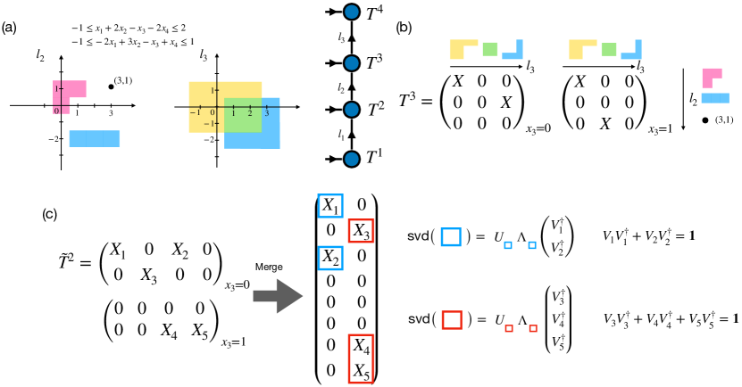
Figure 1: Overview of the main contributions of this work. (a): Given a set of $M$ linear constraints, we encode the entire space of feasible solutions in a new family of matrix product states (MPS), which we dub constrained MPS, and whose link indices are parameterized by $m\leq M$ dimensional regions, QRegions. Shown an example with two inequalities. (b): MPS tensors are quasi block-sparse with blocks arranged according to a fusion rule for QRegions (see main text). (c): Constrained MPS afford a novel canonical form where tensor blocks are factorized jointly according to the fusion rule (to be contrasted with $U(1)$ symmetric tensors whose blocks are factorized independently). Such canonical form allows for efficient optimization algorithms, such as the one developed in this work.

II Symmetric Tensor Networks and Quantum Numbers

In this section we give a brief introduction to $U(1)$ symmetric matrix product states (MPS) and explain how do they relate to linear equations of the form $\mathbf{A}{\bm{x}}={\bm{b}}$. We present two ways of viewing this encoding of linear equations into an MPS: a conceptual one based on finite state machines, and a more procedural one based on backtracking, a method widely used in constraint programming. For more details on the connection between linear equations and tensor networks we refer to Ref. Lopez-Piqueres et al. (2022), as well as the original work by Singh et al. on the general theory of $U(1)$ symmetric tensor networks Singh et al. (2011).

II.1 Introduction to $U(1)$ symmetric matrix product states

While a common perspective is to view tensors appearing in MPS as mere multidimensional arrays, for discussing block-sparse tensors that arise from equalities like the one above, it is helpful to take the perspective of representation theory. In this regard, we view each tensor as a linear map between an input $\mathbb{V}^{\rm in}$ and output vector space $\mathbb{V}^{\rm out}$. This can be visualized by assigning arrows to each index of each tensor, e.g.

A well-known result from representation theory dictates that, if such linear transformation is symmetric w.r.t. to a generic, compact group $\mathcal{G}$, it must map between states of fixed irrep. Each irrep is labeled by a well-defined charge or quantum number (QN), $n_{i}\in\mathbb{N}$. If tensor $T$ is symmetric w.r.t. $U(1)$, then

$$U_{\alpha}^{\dagger}\otimes U_{a}^{\dagger}\otimes U_{\beta}T=e^{-in\phi}T,$$ (2)

with $U_{x}=e^{-in_{x}\phi}$, with $\phi\in[0,2\pi)$, and $n_{x}\in\mathbb{N}$ denoting the charge of irrep $\mathbb{V}_{n_{x}}$ of $\mathbb{V}_{\rm in,out}$, and we are taking the transpose conjugate of the representation $U_{x}$ when acting on input states. The integer $n$ denotes the total charge of the tensor, which is an integer and satisfies $n_{\beta}-n_{a}-n_{\alpha}=n$. Because of this property, the total charge is also known as the flux: i.e. the sum of outgoing minus incoming charges must match the total charge. The upshot is that $U(1)$ symmetry induces a block-sparse structure on $T$, with blocks labeled by charges fulfilling the charge conservation condition. Moreover, each block can be of any dimension, since each irrep $n_{i}$ can be of dimension $d_{n_{i}}$.

This formalism can be applied to higher dimensional tensors, such as MPS. In particular, an MPS is $U(1)$ symmetric if each of its tensors transforms as in Fig. (2). When an MPS is charged, its global charge or flux is usually carried by one of the tensors alone, denoted as the flux tensor. Moreover, when the MPS is in canonical form Schollwöck (2011), it is also customary to assign such tensor as the canonical tensor.

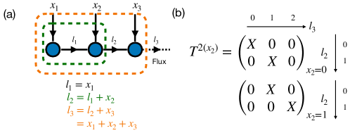
Figure 2: $U(1)$ symmetric MPS. (a) Charge conservation in $U(1)$ symmetric MPS. Each physical (vertical) index carries a charge $x_{i}\in\{0,1\}$. The charge conservation of the dashed green and orange regions can be guaranteed by local tensor conservation. The sum of all local charges must match the total charge or flux of the MPS, shown in dashed line. (b) The block structure of tensor at the second site, with each $X$ an unspecified block.

When tensors in an MPS collectively satisfy the charge conservation condition, contracting these tensors together maintains global conservation. As demonstrated in Fig. 2(a), the input charge equals the output charge across each local region, ensuring that the overall system respects $U(1)$ charge conservation.

All in all, by leveraging $U(1)$ symmetric tensor networks, we guarantee computational savings, since each tensor will be block-sparse (Fig. 2(b)).

II.2 Encoding arbitrary equality constraints in $U(1)$ symmetric matrix product states

Following our introduction to $U(1)$ symmetric matrix product states, we now explore their application in encoding the feasible solution space of linear equations. We transition from using specific charge indices $n_{i}$ to a more general labeling $l_{i}$ for link charges. Consider an equality constraint of fixed cardinality:

$$x_{1}+x_{2}+x_{3}=2,\quad x_{i}\in\{0,1\}$$ (3)

This constraint mirrors constraints in quantum many-body physics, such as particle number conservation in bosonic systems or magnetization in spin chains, where the total number or magnetization remains fixed.

To construct the MPS corresponding to this equation we set the flux of the MPS of value $2$ at the last site and set out to determine the charges on all links, $l_{i}$, consistent with charge conservation. This process can be conceptually likened to a finite state machine (FSM), where each link charge $l_{i}$ represents the state at step $i$, and each $x_{i}$ serves as the input at that step, see Fig. 3.

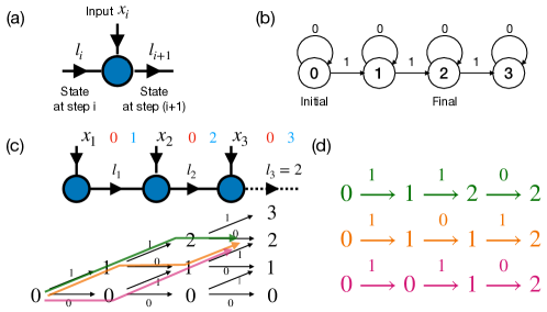
Figure 3: Charge conservation as a finite state machine (FSM). (a) The charge on each link is associated with a state. (b) We can view such states and their transitions as being part of a FSM. Shown here a FSM with final state 2. (c) (Top) MPS with flux 2 at the last link. Red/blue numbers on top of each link denote cumulative lower/upper bounds as we go left-to-right. (Bottom) If the finite state is constrained to $2$, there are in total three transition paths colored by green, orange and purple. (d) Each of these paths corresponds to one feasible solution bitstring to $x_{1}+x_{2}+x_{3}=2$.

The state transitions within this FSM are dictated by the conservation of charge:

• If $x_{i}=0$, the state remains unchanged ($l_{i+1}=l_{i}$).

• If $x_{i}=1$, the state advances ($l_{i+1}=l_{i}+1$).

To ensure the FSM concludes at $l_{3}=2$, various paths (colored in green, orange, and purple in Fig. 3(c)) represent all valid transitions from $l_{0}=0$ to $l_{3}=2$, corresponding to bit strings 110, 101, and 011.

We present now an effective method to derive link charges. This involves:

• Determining Bounds: Establish cumulative lower and upper bounds on the charge at each link, as illustrated in Fig. 3(c) in red and blue.

• Recursive Solution: Begin with the boundary condition $l_{3}=2$ and recursively solve backwards $l_{i}+x_{i+1}=l_{i+1}$. For instance, from $l_{3}=2$ and potential $x_{3}$ values, derive possible $l_{2}$ values within bounds.

• Consistency Check: In general, another forward pass from the left end is needed to remove all quantum numbers that are not consistent with the boundary condition $x_{1}=l_{1}$.

This analysis can be carried out for any type of linear equation, and in fact, for any number of them Lopez-Piqueres et al. (2022). This procedure bears resemblance to backtracking in the context of constraint programming, where solutions are explored systematically, reverting if constraints are violated. Crucially, however, our approach constructs the solution space indirectly by determining the relevant charges rather than directly computing all possible solutions. In the $U(1)$ symmetric MPS framework, this method involves defining link charges $l_{i}$ that are consistent with global charge conservation. Since the number of local unique charge configurations $\{l_{i}\}$ is generally fewer than the total number of potential solutions $\{{\bm{x}}|\mathbf{A}{\bm{x}}={\bm{b}}\}$, our method benefits from a more efficient encoding of the solution space, compared to traditional backtracking, which must consider each possible solution independently.

III Constrained Tensor Networks and Quantum Regions

In this section, we generalize the formalism of $U(1)$ symmetric MPS to inequality constraints by introducing the concept of QRegion, short for Quantum Region. This consists of a group of QNs in the $M$-dimensional hyperplane (for $M$ constraints) effectively describing each link charge in the MPS. We start with a one inequality example of cardinality type and explain the motivation and benefits of grouping QNs into QRegions. As in the equality case, we provide two perspectives to the QRegion finding process: one conceptual based on FSMs and a procedural one based on backtracking. We then show how can we generalize these results in the presence of multiple inequalities, and present one of the main results of this work, captured by Algorithms 1 and 2 for constructing MPS from arbitrary linear constraints. We dub this new family of MPS constrained MPS.

III.1 One inequality

Having demonstrated the computational advantages of utilizing $U(1)$ symmetric TNs for managing equality constraints, we now shift our focus to inequality constraints. A prevalent technique, widely used in the context of quadratic unconstrained binary optimization (QUBO) problems, involves transforming each inequality into an equality by incorporating slack binary variables Glover et al. (2019). Using this method, the number of extra binary variables grows with the number of inequalities, potentially increasing the complexity of the tensor network ansatz.

We propose here a more direct approach that encodes inequalities directly within the network’s architecture, thereby reducing both the number of binary variables and potentially the bond dimension of the tensor network. Our approach is inspired by $U(1)$ symmetric TNs. Consider the inequality:

$$2\leq x_{1}+x_{2}+\cdots+x_{6}\leq 4.$$ (4)

Rather than treating potential $U(1)$ fluxes separately for each case within the bounds, we encode them as a single interval $[2,4]$.

Finite State Machine Approach: We utilize a FSM strategy to dynamically manage the state transitions based on the sum $x_{1}+x_{2}+\cdots+x_{i}$. This approach, illustrated in Figure 4, allows for an early-stop strategy. This strategy halts computations when the constraints are definitively satisfied or violated, thereby avoiding unnecessary calculations. In our analysis, the cumulative lower and upper bounds correspond to setting all $x_{i}=0$ and $x_{i}=1$, respectively.

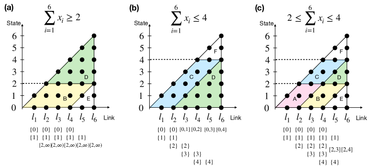
Figure 4: Possible states of FSM of each link index with different constraints. (a) Inequality $\sum_{i=1}^{6}x_{i}\geq 2$. (b) Inequality $\sum_{i=1}^{6}x_{i}\leq 4$. (c) Inequality $2\leq\sum_{i=1}^{6}x_{i}\leq 4$. In each of these panels we show the set of allowed QNs at each link, and group them into a segment if they fall within the region shaded in green. All regions fall within the cumulative lower and upper bounds, indicated by the right triangle. More details on the meaning of each colored region is provided in the main text.

In view of a FSM, $l_{0}=0$ is the initial state, and the transition between states satisfying $l_{i}=l_{i-1}+x_{i}$. Since each $x_{i}\in\{0,1\}$, we have $0\leq l_{i}\leq i$, which is in the triangular region with all values shown by points in Fig. 4. The boundary of which is provided by the cumulative upper and lower bound in Eq. 4 as we go from the first bit $x_{1}$ to the last $x_{6}$. In Fig. 4 we show three kinds of inequalities: Fig. 4(a) with only lower bound, 4(b) with only upper bound, and 4(c) with both lower and upper bound.

In (a) and following the early-stop policy, once the $l_{i}$ reaches $2$, the constraint is unconditionally fulfilled. So we group any quantum numbers larger than $2$ into one object, the segment $[2,\infty)$. The corresponding region in (a) is labelled by the green region and symbol D. In contrast, the points in white E region would violate the constraint whatever the remaining $x_{i},x_{i+1},\cdots,x_{6}$ values are. The yellow region in B consist of charges that may or may not end up fulfilling the global constraint as this will depend on the remaining bits, so we cannot resolve them and we need to keep them all separate.

Similarly, in (b) we plot the case when only the upper bond constraint is considered. As long as the charge $l_{i}\leq i-2$, we’re guaranteed to fulfill the constraints. If by any chance, it enters the white F region, then it would already violate the constraint. Analogous to the yellow B region in (a), blue C region consists of charges that may or may not fulfill the global constraint so we cannot a priori group them.

If we combine these two cases together, and consider both constraints at the same time, we get panel (c). In this case we get the same colored regions as in panels (a) and (b), as well as a new region A in red, which is the intersection of regions B and C and is composed by QNs that cannot automatically be grouped. The goal is the finite state $l_{6}$ to stay in the interval $[2,4]$. The color code means the same as (a) and (b). The B (C) region means the upper (lower) bound is guaranteed to fulfill whatever the following $x_{i}$, however the lower (upper) bound is undetermined. So in B and C region, half side of the constraints are fulfilled while the other half depends on the remaining $x_{i}$ inputs.

Backtracking Approach: Let us now show how these different regions are defined and segmented. Starting from the right-most link index $l_{6}$ and going to the first link index $l_{1}$, we call this step backward decomposition sweep, since the original segment $l_{6}=[2,4]$ is broken into smaller segments as we go left. To see this, we first resolve the relationship $l_{5}\subseteq l_{6}-x_{6}$. This computation yields two scenarios based on the values of $x_{5}$: for $x_{5}=0$, $l_{5}^{(x_{5}=0)}=[2,4]$; for $x_{5}=1$, $l_{5}^{(x_{5}=1)}=[1,3]$. So $[2,4]$ and $[1,3]$ have some overlaps, while also differences. So it’s reasonable to split the interval into a disjoint union of non-overlapping and overlapping segments. This guarantees computational savings by grouping overlapping terms. In this case, we get ${1}$, $[2,3]$, ${4}$. These belong to regions B (yellow), D (green) and C (blue) regions, respectively. These three items form $l_{5}$, i.e. $l_{5}=\{1,[2,3],4\}$. Hence the original segment $[2,4]$ has been broken into smaller pieces. In an analogous way we find the remaining links $l_{i<5}$.

A similar decomposition into colored regions occurs for arbitrary lower/upper bounds. Two edge cases are relevant. Let the range $\Delta=u-l$ with $u,l\geq 0$ the upper/lower bound. When $\Delta=0$ we recover the $U(1)$ symmetric case discussed in the previous section, and the B, C, D regions vanish, leaving only regions A, E, F. In that case, we need to keep track of each individual QN and cannot group them. On the opposite limit, when we enlarge the bounds and $\Delta=\infty$, then the D region absorbs the other regions (A through F). This means there is actually no constraint and the corresponding MPS is the trivial product state with effectively a single segment at each link (of value $[0,\infty)$). These sanity checks reinforce the idea that the presented approach is efficient.

This approach extends to any inequality of the form $l\leq\sum_{i}a_{i}x_{i}\leq u$, even with non-positive coefficients, where cumulative lower bounds might be negative. Each site index modifies the initial flux region, breaking it down into smaller segments as we move backward from the last tensor in the network. We will refer to these segments and the associated quantum numbers collectively as quantum regions, or QRegions. This terminology will become clearer as we explore scenarios involving multiple inequalities.

One remark which is not apparent in the inequality discussed above is that the backward decomposition sweep only gives a (super)set of potential QRegions. For generic inequalities a further forward validation sweep is needed starting from the left-most link. This guarantees that only those QRegions consistent with the relation $l_{i}+a_{i+1}x_{i+1}\subseteq l_{i+1}$ and the left boundary condition $l_{1}=a_{1}x_{1}$ are kept. This is because the backward decomposition sweep has only partial information about the left hand side (through the cumulative bounds), and a further sweep is needed to resolve those potential QRegions that could a priori appear from the backward sweep. The corresponding tensors in the MPS will be block-sparse with blocks labeled by QRegions satisfying $l_{i}+a_{i+1}x_{i+1}\subseteq l_{i+1}$.

Lastly, for context we compare the savings that result from our approach when compared with the slack variable approach. For concreteness we consider the inequality constraint $\sum_{i=1}^{6}x_{i}\leq 4$. Converting this to an equality necessarily involves the introduction of three slack variables $s_{i}$ so that the constraint becomes $\sum_{i=1}^{6}x_{i}+s_{1}+2s_{2}+4s_{3}=4$. A simple calculation reveals that the maximum set of QNs for the corresponding symmetric MPS is 5 and the total number of blocks summed over all tensors is 48. In contrast, the maximum set of QRegions in our approach is 3 (as shown in Fig. 4(b)) and the total number of blocks is 26.

III.2 Multiple inequalities.

In the presence of $M\geq 2$ inequalities of the form ${\bm{l}}\leq\mathbf{A}{\bm{x}}\leq{\bm{u}}$ a similar logic follows to that of the one inequality case. Each QN is represented by a tuple of integers $(q_{1},q_{2},\cdots,q_{M})$, which corresponds to a point in the $M$-dimensional hyperplane. The upper and lower constraints define a hyperrectangle or box $l_{N}=\{{\bm{v}}\in\mathbb{N}^{M}:l_{i}\leq v_{i}\leq u_{i}\}$. This is set to be the flux of the whole MPS. The QRegions are defined by a group of QNs in the $M$-dimensional plane, or alternatively, by a disjoint union of connected regions surrounding QNs. This latter perspective will be the one we will use as it requires less bookkeeping and is more intuitive.

In the backward decomposition process the goal is to find the set of potential QRegions at each link index that recursively satisfy $l_{i}\subseteq l_{i+1}-A_{i+1}x_{i+1}$, with $A_{i+1}$ the $i+1$’th column of $\mathbf{A}$ subject to the cumulative bounds constraint. Here the operand $\subseteq$ acts similar to the subset discussed in the one inequality example above: for any QRegion $q\in l_{i}$ there must exist a QRegion in $\tilde{q}\in l_{i+1}-A_{i+1}x_{i+1}$ s.t. $q\subseteq\tilde{q}$.

Initialization algorithm. To find the set of QRegions fulfilling the subset constraint, we introduce two operands acting on a pair of QRegions: the intersection $\cap$, and symmetric difference $\triangle$. A visual description on how they act is shown in Fig. 5 for two QRegions corresponding to boxes in $M=2$. The same operands can be straightforwardly generalized to any set of QRegions, and in higher dimensions, $M>2$.

Figure 5: Basic QRegion operations. Given QRegions $qr_{1}$ and $qr_{2}$, shown here their intersection $qr_{1}\cap qr_{2}$ and their symmetric difference $qr_{1}\triangle qr_{2}$. Together they give three new QRegions, $qr_{1}^{\prime}$, $qr_{2}^{\prime}$, $qr_{3}^{\prime}$.

The backward decomposition sweep is as follows. As in the inequality case above, we first extract the cumulative upper/lower bounds and store that as a vector, $\mathcal{B}$. This is achieved by the function Boundary. Next we compute the last link index, which is found by the intersection between the flux Box$({\bm{l}},{\bm{u}})$ and the cumulative upper/lower bound at the flux link, $\mathcal{B}_{N}$. Next, for $N-1$ iterations we extract $l_{N-i}$ from $l_{N-i+1}$ and $A_{N-i+1}$ as follows. Compute $l_{N-i}^{(0)}=l_{N-i+1}\cap\mathcal{B}_{N-i}$ and its shifted version, $l_{N-i}^{(1)}=(l_{N-i+1}-A_{N-i+1})\cap\mathcal{B}_{N-i}$. Compute the intersection of these two indices, $l_{\cap}=l_{N-i}^{(0)}\cap l_{N-i}^{(1)}$, and their symmetric difference $l_{\triangle}=l_{N-i}^{(0)}\triangle l_{N-i}^{(1)}$. Finally, append these two outcomes to extract the new index, $l_{N-i}=l_{\cap}\oplus l_{\triangle}$. Here we overload the $\oplus$ operand to indicate that under the hood, we are decomposing a space into the disjoint union of QRegions from $l_{\cap}$ and $l_{\triangle}$, analogous to how a vector space decomposes into a disjoint sum of irreps labeled by QNs in $U(1)$ symmetric tensors.

Next we perform a forward validation sweep and discard those QRegions found on the backward decomposition sweep that are not consistent with charge conservation. Specifically, starting from the leftmost index we check whether the quantum numbers $0$, $A_{1}$ belong to $l_{1}$ and keep the corresponding QRegions to which they belong as the new $l_{1}$. At the following steps we check which QRegions from $l_{i+1}$ fulfill $l_{i}\subseteq l_{i+1}$ or $(l_{i}+A_{i+1})\subseteq l_{i+1}$, and keep those as forming the new $l_{i+1}$. In this regard, it is useful to introduce the function $\chi(\cdot)$. For any pair of indices $A$ and $B$, $\chi(A\subseteq B)$ returns a new index $B$ with all QRegions in $B$ for which there exists at least one QRegion in $A$ s.t. $q_{A}\subseteq q_{B}$ with $q_{B}\in B$.

Algorithm 1: Constraints to Indices Constraints_to_Indices
Input     Linear constraints $\{\mathbf{A},{\bm{l}},{\bm{u}}\}$
Output     Indices $l_{i}$ 1:$\mathcal{B}_{i=1,2,\cdots,N}\leftarrow\textsc{Boundary}(\mathbf{A})\lx@algorithmicx@hfill\left(\triangleright\right)\text{Compute cumulative lower/upper bounds}$ 2:$l_{N}=\textsc{Box}({\bm{l}},{\bm{u}})\cap\mathcal{B}_{N}$ 3:for $1\leq i<N$ do $\lx@algorithmicx@hfill\left(\triangleright\right)\text{Backward decomposition sweep}$ 4:     $l_{N-i}^{(0)}\leftarrow l_{N-i+1}\cap\mathcal{B}_{N-i}$ 5:     $l_{N-i}^{(1)}\leftarrow(l_{N-i+1}-A_{N-i+1})\cap\mathcal{B}_{N-i}$ 6:     $l_{\cap}\leftarrow l_{N-i}^{(0)}\cap l_{N-i}^{(1)}$ 7:     $l_{\triangle}\leftarrow l_{N-i}^{(0)}\triangle l_{N-i}^{(1)}$ 8:     $l_{N-i}\leftarrow l_{\cap}\oplus l_{\triangle}$ 9:end for 10:$l_{1}\leftarrow\chi(0\subseteq l_{1})\oplus\chi(A_{1}\subseteq l_{1})$ 11:for $1\leq i<N$ do $\lx@algorithmicx@hfill\left(\triangleright\right)\text{Forward validation sweep}$ 12:     $l_{i+1}\leftarrow\chi(l_{i}\subseteq l_{i+1})\oplus\chi((l_{i}+A_{i+1})\subseteq l_{i+1})$ 13:end for Return     $l_{i}$.

Example. To illustrate the initialization algorithm for multiple inequalities, we consider the following two inequalities:

$$\begin{split}-1&\leq x_{1}+2x_{2}-x_{3}-2x_{4}\leq 2\\ -1&\leq-2x_{1}+3x_{2}-x_{3}+x_{4}\leq 1.\end{split}$$ (5)

The corresponding constrained MPS is depicted in Fig. 6, where, as before, we’ve denoted by red/blue numbers the cumulative lower/upper bounds of charge on $l_{i}$ w.r.t. each inequality. The backward decomposition sweep is illustrated in Fig. 7. It starts from the flux of the MPS at the last tensor, given by $l_{4}=[(-1,-1),(2,1)]$, which is a rectangle defined by the down-left and top-right corner in the format $[(x_{\text{1,min}},x_{\text{2,min}}),(x_{\text{1,max}},,x_{\text{2,max}})]$, plotted as a green rectangle in Fig. 7(a). We define $Q_{i}$ as the number of QRegions in $l_{i}$. So $Q_{4}=1$ since it contains only one QRegion. The link index $l_{3}$ is found by the intersection and symmetric differences from lines 6, 7 of Algorithm 1, with the boundary $\mathcal{B}_{3}=[(-1,-3),(3,3)]$. This results in $l_{\cap}=[(1,-1),(2,0)]$ and $l_{\triangle}=\{[(-1,-1),(0,0)]\cup[(-1,1),(2,1)],[(1,-2),(3,-2)]\cup[(3,-1),(3,0)]\}$. Using line 8 of Algorithm 1 we get $l_{3}=l_{\cap}\oplus l_{\triangle}=\{[(1,-1),(2,0)],[(-1,1),(2,1)],[(1,-2),(3,-2)]\cup[(3,-1),(3,0)]\}$, which is a link index with three QRegions, thus $Q_{3}\leq 3$. The upper bound being since some of these QRegions may ultimately not appear upon implementing the forward validation sweep. Visually $l_{3}$ corresponds to Fig. 7(b) where the different QRegions are shaded in yellow, blue (symmetric difference) and green (intersection). We note that QRegions such as the L-shape in yellow or blue can be represented as the union of disjoint boxes. This is in fact how we encode arbitrary QRegions in code.

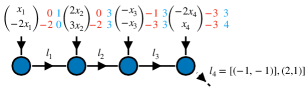
Figure 6: Constrained MPS with flux at last site. Corresponding to Eq. (5).

The remaining indices can be found in an analogous manner yielding visually Fig. 7(c-d). From (c) we see that $l_{2}$ consists of multiple pieces, most of which contains only one QN in its QRegion. For ease of exposition, we call these QNs as QRegions. These special QRegions are not colored for simplicity in (c) or (d). So $l_{2}$ contains three regular and nine special QRegions (QNs), with a total of twelve QRegions.

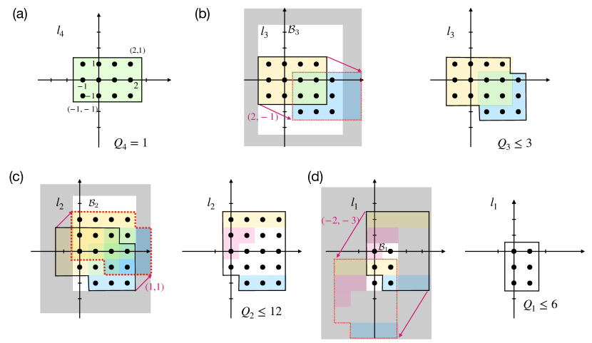
Figure 7: Backward decomposition sweep. Here shown for the two inequalities of Eq. 5. $Q_{i}$ is the number of QRegions for link index $l_{i}$. Since this is only the backward sweep, the actual number of QRegions can be smaller. (a) The feasible QRegion of $l_{4}$ is given by the green area. (b,c,d) QRegions at links $l_{3}$, $l_{2}$, $l_{1}$, respectively. The gray area is beyond the boundary $B_{i}$ of possible values. The pink arrow is given by $-A_{i}$, from step 5 of Algorithm 1.

Once the backward process is over the next step is to proceed with the forward validation process, lines 10-13 in Algorithm 1. Starting from the boundary condition $l_{1}=A_{1}x_{1}$, we check which QRegions in $l_{i+1}$ fulfill $l_{i}+A_{i+1}x_{i+1}\subseteq l_{i+1}$. This process selects the QRegions shown in Fig. 8(a-d), with max $Q_{i}=3$. The black dots correspond to the QNs that would be selected had we instead solved $\hat{l}_{i+1}=\hat{l}_{i}+A_{i+1}x_{i+1}$ subject to $\hat{l}_{i+1}\subseteq l_{i+1}$ with $\hat{l}_{1}=A_{1}x_{1}$. In that case the number of QNs at site 3 and 4 are $Q_{3}=Q_{4}=4$ which is greater than the maximum number of QRegions. Hence, by working with QRegions we guarantee the most compact representation of a constrained MPS. We remark that we are including QNs into each QRegion that are never part of the solution space (such as $(0,-1)$ at link index $l_{3}$). The reason for the introduction of these virtual QNs is to ease the representation of each QRegion. For instance, instead of considering $l_{4}$ as the union of the four black dots in Fig. 8(d), it is simpler to consider the green rectangle in its entirety, thereby storing only two coordinates for the corners of the rectangle, as opposed to four for the dots.

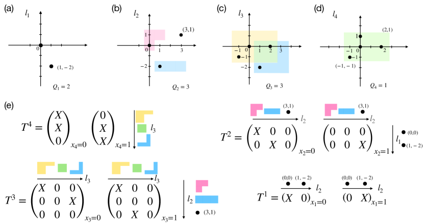
Figure 8: Forward validation sweep. Here shown for the two inequalities of Eq. 5. (a-d) QRegions extracted in the forward validation sweep solving using lines 10-13 of Algorithm 1. The dots denote the QNs within each QRegion that in actuality are selected – see main text. (f) The block-sparse tensor structures for all tensors in the MPS. Each column and row are labeled by its corresponding QRegion. The meaning of the color and shape is the same as in panels (a-d).

The above analysis assumed that the flux was placed at the last tensor. Moving the flux center in $U(1)$ MPS is straightforward and can be done dynamically by solving the equality constraint $qn_{\text{left}}+qn_{\text{right}}+\alpha x=\rm flux$, with $\alpha\in\mathbb{N}$ and $x\in\{0,1\}$ the site index QN. In particular, if we move the flux tensor from site $i$ to site $i+1$, we only need to solve for $qn_{\rm left}$; see Sec. II. In contrast, for constrained tensors involving arbitrary QRegions, the flux condition becomes $qr_{\text{left}}+qr_{\text{right}}+\alpha x\subseteq\rm flux$. This condition is ambiguous if we were to solve say for the set of QRegions on the left index. In order to determine it, we need to find the QRegions when fixing the flux at the first site, which results in the MPS of Fig. 9.

Letting $\tilde{l}_{i}$ the set of link indices resulting from placing the flux at the first site and applying Algorithm 1 with $\mathbf{A}$ reversed (so that $A_{i}\leftrightarrow A_{N-i+1}$), yields the following QRegions $\tilde{l}_{1}=\{[(-2,2),(1,3)]\cup[(-2,1),(-2,1)],[(-1,-1),(2,0)]\cup[(2,1),(2,1)]\}$, $\tilde{l}_{2}=\{[(0,-1),(0,0)],[(-1,-1),(-1,0)],[(-2,1),(-2,1)],[(-3,-1),(-2,0)]\}$, $\tilde{l}_{3}=\{[(0,0),(0,0)],[(-2,1),(-2,1)]\}$. Note in particular that $4=|\tilde{l}_{2}|\neq|l_{2}|=3$, and $2=|\tilde{l}_{3}|\neq|l_{3}|=3$.

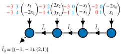
Figure 9: Constrained MPS with flux at first site. Corresponding to Eq. (5).

Away from the edges, the flux tensor will have blocks labeled by QRegions fulfilling $l_{i-1}+\tilde{l}_{i}+A_{i}x_{i}\subseteq\text{flux}=[(-1,-1),(2,1)]$, where the addition of QRegions is understood as follows. For two boxes appearing on each QRegion $\text{box}_{1}=[(x_{\text{1,min}},x_{\text{2,min}}),(x_{\text{1,max}},x_{\text{2,max}})]$ from QRegion 1 and $\text{box}_{2}=[(y_{\text{1,min}},y_{\text{2,min}}),(y_{\text{1,max}},y_{\text{2,max}})]$ from QRegion 2, their addition is done component wise, thus $\text{box}_{1}+\text{box}_{2}=[(x_{\text{1,min}}+y_{\text{1,min}},x_{\text{2,min}}+y_{\text{2,min}}),(x_{\text{1,max}}+y_{\text{1,max}},x_{\text{2,max}}+y_{\text{2,max}})]$.

Fixing the flux at site $m$, we can construct the MPS tensors as in Algorithm 2. For simplicity we set all nonzero blocks to the scalar value 1, corresponding to a uniform superposition of all feasible solutions to the associated set of constraints.

One striking consequence of constrained tensors labeled by QRegions is that in contrast to the $U(1)$ symmetric and vanilla cases (no constraints), the bond dimension at the last link can be of value 3 since the flux $l_{N}=\textsc{Box}({\bm{l}},{\bm{u}})$ and its shift by the last site index can be nonempty, $l_{N}\cap(l_{N}-A_{N})\neq\varnothing$. This can produce three new QRegions as in Fig. 5 for the last link.

Algorithm 2: Constraints to MPS Constraints_to_MPS
Input     Linear constraints $\{\mathbf{A},{\bm{l}},{\bm{u}}\}$, flux site $m$
Output     MPS $\psi\hfill\left(\triangleright\right)\text{Feasible solution space MPS}$ 1:$l_{i}\leftarrow\textsc{Constraints\_To\_Indices}(\mathbf{A},{\bm{l}},{\bm{u}})\lx@algorithmicx@hfill\left(\triangleright\right)\text{Extract MPS indices with flux at leftmost site}$ 2:$\tilde{l}_{i}\leftarrow\textsc{Constraints\_To\_Indices}(\text{reverse}(\mathbf{A}),{\bm{l}},{\bm{u}})\lx@algorithmicx@hfill\left(\triangleright\right)\text{Extract MPS indices with flux at rightmost site}$ 3:for $i<m$ do 4:     $T^{i}_{l_{i},l_{i+1}}\leftarrow 1\lx@algorithmicx@hfill\left(\triangleright\right)\text{Initialize tensor components satisfying }l_{i}+A_{i+1}x_{i+1}\subseteq l_{i+1}$ 5:end for 6:for $m<i<N$ do 7:     $\tilde{T}^{i}_{\tilde{l}_{i},\tilde{l}_{i+1}}\leftarrow 1\lx@algorithmicx@hfill\left(\triangleright\right)\text{Initialize tensor components satisfying }\tilde{l}_{i+1}+A_{i+1}x_{i+1}\subseteq\tilde{l}_{i}$ 8:end for 9:$\overline{T}^{m}_{l_{m-1},\tilde{l}_{m}}\leftarrow 1\lx@algorithmicx@hfill\left(\triangleright\right)\text{Initialize flux tensor with components satisfying }\tilde{l}_{m}+l_{m-1}+A_{m+1}x_{m+1}\subseteq\textsc{Box}({\bm{l}},{\bm{u}})$ Return     $\psi=T^{1}_{l_{1}}T^{2}_{l_{1},l_{2}}\cdots T^{m-1}_{l_{m-2},l_{m-1}}\overline{T}^{m}_{l_{m-1},\tilde{l}_{m}}\tilde{T}^{m+1}_{\tilde{l}_{m},\tilde{l}_{m+1}}\cdots\tilde{T}^{N-1}_{\tilde{l}_{N-2},\tilde{l}_{N-1}}\tilde{T}^{N}_{\tilde{l}_{N-1}}$.

IV Complexity of Constrained Tensor Networks

Having discussed the construction of constrained tensor networks for arbitrary linear constraints we study now the complexity of Algorithm 1. The bottleneck of the algorithm occurs at steps 6 and 7. Step 6 finds the intersections among all pairs of QRegions appearing on indices $l_{N-i}^{(0)}$ and $l_{N-i}^{(1)}$. Each QRegion is in turn composed of a disjoint union of boxes. Thus, at the most basic stack one performs the intersection of two boxes, which scales as $\mathcal{O}(M)$, with $M$ the number of constraints. Step 7 is also dominated by the intersection of pairs of QRegions. The number of such intersections will be ultimately determined by the specific constraints. In general, we do observe that the more structure there is in the constraints (as measured e.g. by the variance of coefficients), the fewer QRegions there will be. The dependence of the intersection step on the number of constraints has an impact on the complexity of the algorithm. The natural measure of complexity in this setup is the maximum number of QRegions across all tensors, and among both the MPS with flux at either end. We dub this quantity charge complexity, denoted by $Q$.

Note that each QRegion could be composed of multiple boxes, which adds complexity, but since the rank of each tensor is determined by the number of QRegions, we choose this quantity instead. In general we observe that for dense constraint matrices $\mathbf{A}$, the scaling of $Q$ is exponential in $M$, but polynomially in the number of bits $N$ for constraints with well enough structure. The dependence on both $N$ and $M$ is illustrated below for a family of constraints that arise in a version of the facility location problem.

Charge complexity for cardinality constraint. While we do not have guarantees that our constrained tensor network construction is optimal, we give an intuition that this is so for a simple constraint, given by $l\leq\sum_{i}x_{i}\leq u$. Suppose we want to describe the TN corresponding to an inequality with no lower or upper bounds (i.e. $l=-\infty$ and $u=\infty$, for lower and upper bounds, respectively). The smallest rank TN representation for this problem, corresponding to setting all TN blocks to be of size one, is given by a trivial product state. When $u=l=N/2$, the charge complexity is given by $Q=N/2+1$ Lopez-Piqueres et al. (2022). In between these two limits the charge complexity scales linearly with the range $\Delta=u-l$. In Fig. 10 we show this for a specific set of $\Delta$ parameterized as $\Delta_{i}=u_{i}-l_{i}$, $i=0,1,2,\cdots$, with $u_{i}=N/2+i$, $l_{i}=N/2-i$. In Fig. 10 we show via a scaling collapse that the complexity for this particular example in fact scales sublinearly as $Q<N$. In fact, the maximum complexity as a function of the range $\Delta$ corresponds to $Q(\Delta^{*})\approx 0.67N$, with $\Delta^{*}=0.36N$.

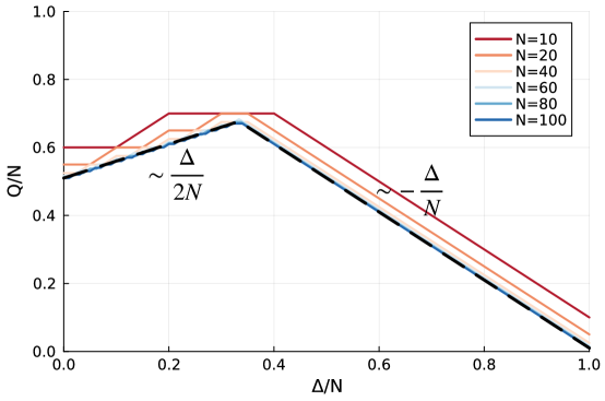
Figure 10: Charge complexity for cardinality constraint. Scaling collapse of charge complexity vs range for cardinality constraint. The maximum complexity occurs at a value roughly at $\Delta^{*}\approx 0.34N$ with complexity $Q\approx 0.67N$ (i.e. sublinear).

Charge complexity for facility location problem. The facility location problem is a classic optimization problem in operations research and supply chain management. The goal is to determine the most cost-effective locations for facilities (e.g., warehouses, factories, retail stores) and to allocate demand points (e.g., customer locations, market areas) to these facilities to minimize overall costs while satisfying service requirements. Here we model the set of constraints appearing in this problem by a set of inequality constraints of the form:

$$l\leq\sum_{j\in\text{Facilities}}x_{i,j}\leq u\text{, }i=1,2,\cdots,M.$$ (6)

Here $M$ is the number of demand points. For concreteness we fix $l=2$, i.e. two facilities must serve each demand point at any given time, and let the maximum number of facilities per demand point $u$ vary. Furthermore, each demand point is served by 10% of the facilities, chosen randomly. All in all, the constraint matrix $A$ is an $M\times N$ matrix whose entries are in $\{0,1\}$ such that $\sum_{j}A_{i,j}=\lfloor 0.1N\rfloor$. The locations of $A_{i,j}=1$ are chosen randomly.

In Fig. 11 we show the charge complexity as a function of the number of bits $N$ for different number of constraints $M$ for $u=2$ (minimum), $u=3$, and $u=10$ (maximum). For each tuple of $(N,M,u)$ we construct 5 different constraint matrices $A$ as above and extract the statistics of the charge complexity (mean and standard error), remarking that the results are not very sensitive to the specific choice of matrix $A$. The results show that the charge complexity scales polynomially as a function of $N$ for fixed set of constraints. Furthermore, the results for minimum number of facilities per demand point, $u=2$, show a similar charge complexity to that of the maximum number of facilities per demand point, $u=10$. This shows that our constrained tensor network ansatz captures efficiently inequality constraints of large range (to be contrasted with the slack variable method where the complexity as measured by the addition of slack bits increases with the range). We also show that the charge complexity increases exponentially as a function of number of constraints $M$ for fixed $N$. Finally we show the charge complexity as a function of the upper bound $u$ for fixed $N$ and $M$. The behavior is consistent with that of the cardinality example discussed above: the complexity increases polynomially up to some range $\Delta=u-l$, and decreases polynomially beyond that point.

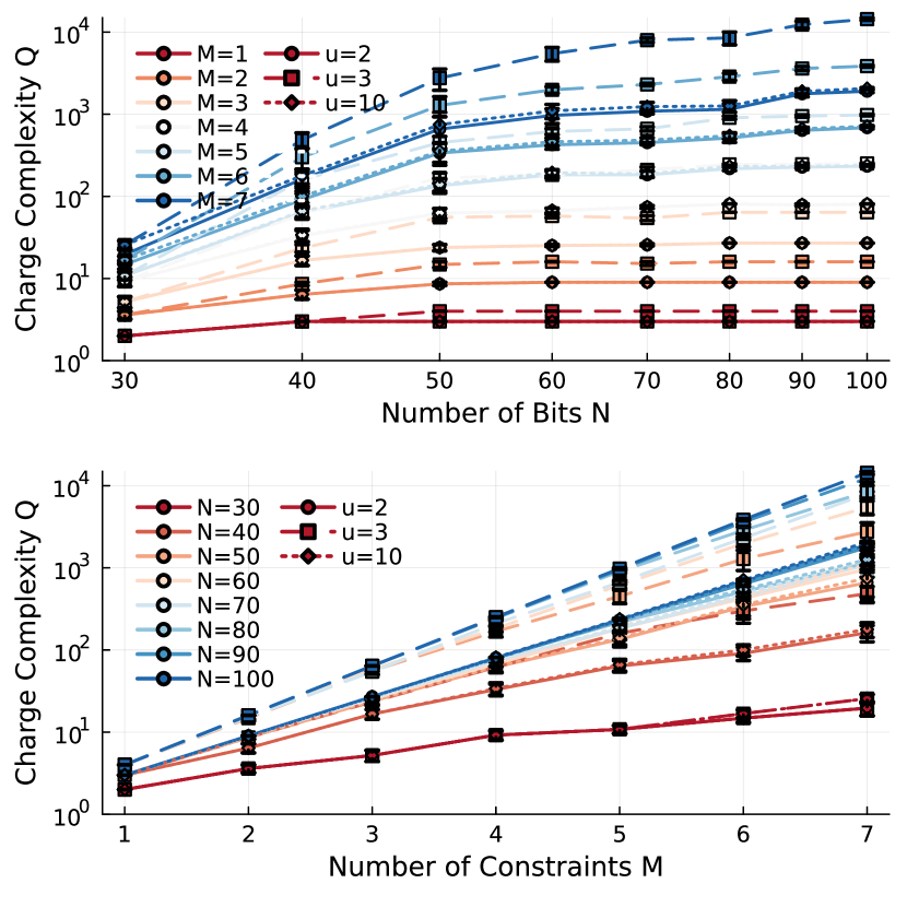
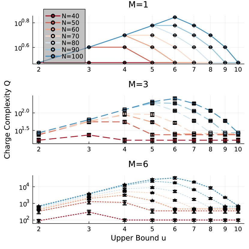
Figure 11: Charge complexity for facility constraints. Top left panel illustrates the charge complexity as a function of the number of bits $N$ for varying numbers of constraints $M$ with upper bounds $u$ set at 2 (minimum), 3, and 10 (maximum). We present data for 5 different constraint matrices $A$ per tuple $(N,M,u)$, showing mean charge complexity and standard error, indicating low sensitivity to the specific matrix $A$. The charge complexity generally exhibits polynomial scaling with $N$ for a fixed set of constraints. Bottom left panel shows the charge complexity as a function of number of constraints $M$ for fixed $N$ and $u$, showing exponential scaling. Right panel examines charge complexity as a function of the upper bound $u$ for constant $N$ and $M$, reflecting a polynomial increase up to a specific range $\Delta=u-l$, followed by a polynomial decrease. This trend parallels the cardinality results discussed previously.

V Canonical Form and Compression

Section III discussed how to find the set of QRegions for an arbitrary set of inequalities. These will be the labels of each block that appear on each tensor in the MPS. A nice property about MPS in general is that they afford a canonical form Schollwöck (2011). This fixes the gauge degree of freedom that arises from equivalent representations of the same MPS, a consequence of the fact that inserting any pair of invertible matrices $P$ and $P^{-1}$ at any link of the MPS leaves the resulting MPS invariant. Among the different choices of gauge, there exists a particular one so that the optimal truncation of the global MPS can be done directly on a single tensor, the canonical tensor.

Canonical forms exist for vanilla and $\mathcal{G}$ symmetric MPS (with $\mathcal{G}$ some arbitrary local or global symmetry group). Here we will show that constrained MPS afford a canonical form as well. Recall that an MPS is canonicalized with canonical center at site $i$ if all tensors to the left of this are left isometries, $\sum_{j=0,1}(T^{(j)})^{\dagger}T^{(j)}=\mathbbm{1}$, and all tensors to the right are right isometries, $\sum_{j=0,1}T^{(j)}(T^{(j)})^{\dagger}=\mathbbm{1}$. Such canonical forms can always be accomplished via a series of orthogonal factorizations such as QR or SVD, leaving the nonorthogonal tensor as the canonical tensor, and the rest being isometries.

In order to canonicalize one must be able to matricize each rank-3 tensor in the MPS, via fusing each site index with one of the virtual indices, followed by splitting after factorization is achieved. Fusing and splitting of indices can be done on $\mathcal{G}$ symmetric tensors via use of Clebsh-Gordan coefficients. For $\mathcal{G}=U(1)$ such coefficients become straightforward and amount to solving linear equations of the form $n_{1}+n_{2}=n_{12}$, with $n_{12}$ the merged index. For constrained tensors arising from inequality constraints fusion and splitting can’t be done in an analogous manner, as each subspace corresponding to a block is labeled by a QRegion and flux conservation dictates $qr_{1}+qr_{2}\subseteq qr_{12}$. Such an undetermined system requires a different strategy.

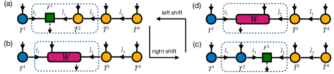
Figure 12: Canonicalization of an MPS. The (a)-(b)-(c) panels explain the right shift of canonical center while (c)-(d)-(a) panels show the left shift of the canonical center. (a) The MPS canonical form. The MPS contains three parts. The green tensor (matrix) is the canonical center defined on link between 1st and 2nd site, which carries the flux. All the blue tensors are the same tensors that appear on the left canonical MPS, while the orange tensors are from the right canonical MPS. (b) If we want to move the canonical center to the right, we first contract $F^{1}$ and $\tilde{T}^{2}$ and get $W$. (c) Then we try to factorize $W$ and get $T^{2}$ and $F^{2}$. At this stage we have successfully moved the canonical center one site to the right. (d) Shows the intermediate state when left shifting the canonical center. The $W$ tensor is the same as in (b), however, it is reshaped into a different matrix (see main text).

The approach taken here is to precompute all link indices by setting the flux of the mps at the first and the last sites, as explained before. This will determine all indices $\{l_{i}\}$ and $\{\tilde{l}_{i}\}$. Suppose we have canonicalized the mps to be at site $i$. It suffices to show how to shift the canonical center from site $i$ to site $i+1$, as depicted in Fig. 12. Here the canonical tensor is denoted in green, which is a flux matrix $F$ defined between $i$ and $i+1$. All tensors in blue on the left $T^{1},T^{2},\cdots,T^{i}$ are the same tensors appearing in the left canonical MPS, while those in orange on the right $\tilde{T}^{i+1},\tilde{T}^{i+2},\cdots,\tilde{T}^{N}$ tensors are the same ones appearing in the right canonical MPS. These tensors satisfy the following condition

In Fig. 12, we show the whole process of shifting the canonical center from $F^{1}$ to $F^{2}$. We first contract the $F^{1}$ and $\tilde{T}^{2}$ tensor into $W$ tensor in (b). Then we factorize and truncate into new tensors $T^{2}$ and $F^{2}$ in (c). The updates only happens locally in the dashed region, which can be captured by the conditions

$$F^{i-1}\tilde{T}^{i}=T^{i}F^{i},$$ (7)

subject to $$F^{0}=F^{N+1}=\mathbbm{1},$$ (8)

$$\sum_{j}\tilde{T}^{i(j)}(\tilde{T}^{i(j)})^{\dagger}=\mathbbm{1}\text{, }l_{i-1}+\tilde{l}_{i-1}\subseteq\phi,$$ (9)

$$\sum_{j}(T^{i(j)})^{\dagger}T^{i(j)}=\mathbbm{1}\text{, }l_{i}+\tilde{l}_{i}\subseteq\phi,$$ (10)

with $\phi$ the flux. These conditions are on top of the ones discussed earlier for each of the tensors away from the flux, i.e. $\tilde{l}_{i}+A_{i}x_{i}\subseteq\tilde{l}_{i-1}$ and $l_{i-1}+A_{i}x_{i}\subseteq l_{i}$. The upshot is that these constraints allow for the following features: 1) The number of blocks at a given tensor is not necessarily preserved when we move the canonical center; i.e. the number of blocks in $T^{i}$ and $\tilde{T}^{i}$ may differ. 2) Relatedly, factorizations may occur on joint blocks. This is a consequence of the fact that two merged indices may have multiple QRegions contained in a given QRegion of a third index. 3) In order to determine which blocks to factorize jointly we need to supplement the factorization with information from the new index that will result from merging. This may incur an increase in complexity, as shown in Fig. 10.

The three index tensor $W\in\mathbb{R}^{\chi_{L}\times d\times\chi_{R}}$ can be matricized by merging the site index with one of the link indices. Considering first the merging with the left index we get $W\in\mathbb{R}^{d\chi_{L}\times\chi_{R}}$, which can then be used to factorize, and if necessary, compress via singular value decomposition (svd). Factorization results in the product of $\bar{U}\in\mathbb{R}^{d\chi_{L}\times\chi}$ and $F\in\mathbb{R}^{\chi\times\chi_{R}}$. The new tensor $T^{2}$ would be the reshape of $\bar{U}$ here:

Notably, $\bar{U}$ is not a square matrix after truncation. $\chi\leq\text{min}(d\chi_{L},\chi_{R})$ is the dimension maintained after truncation. $\bar{U}$ does not carry flux, i.e. we have QRegion conservation and it corresponds to a block diagonal matrix and can be written as $\bar{U}=\oplus_{i=1}^{q}\bar{U}_{i}$, where $\bar{U}_{i}\in\mathbb{R}^{D_{i}\times{\bar{D}_{i}}}$ represent different blocks. The row dimension is not truncated $\sum_{i}D_{i}=\chi_{L}d$, while the column dimension satisfies $\sum_{i}\bar{D}_{i}=\chi$. The orthogonal condition of $\bar{U}$ would require that each $\bar{U}_{i}$ would be an isometry. Our goal is to factorize $W$ so that the norm-2 error is as minimal as possible subject to the canonical condition of $\bar{U}$ in Eq. 10.

$$\bar{U}_{i},\bar{F}=\text{argmin}(\left\|W-\bar{U}\bar{F}\right\|^{2})\quad\text{s.t.}\quad\bar{U}^{\dagger}_{i}\bar{U}_{i}=I_{i}\quad\forall i$$ (11)

For convenience, we use symbol with bars to represent truncated matrix or tensors in our discussion.

We will give the solution of the optimization directly in the following. The proof is provided in Appendix A.

Solution. We split $W\in\mathbb{R}^{d\chi_{L}\times\chi_{R}}$ along the row dimension, and get the vertical concatenation of $W_{i}\in\mathbb{R}^{D_{i}\times\chi_{R}}$

$$W=\begin{pmatrix}W_{1}\\ W_{2}\\ \vdots\\ W_{q}\end{pmatrix}$$ (12)

The division of the row dimension depends on row of $\bar{U}$. Then we factorize each $W_{i}$ by svd, and get

$$W_{i}=\bar{U}_{i}\bar{\Lambda}_{i}\bar{V}_{i}^{\dagger}$$ (13)

where $\bar{U}_{i}\in\mathbb{R}^{D_{i}\times\bar{D}_{i}}$, $\bar{\Lambda}_{i}\in\mathbb{R}^{\bar{D}_{i}\times\bar{D}_{i}}$ is diagonal matrix, $\bar{V}_{i}\in\mathbb{R}^{\chi_{R}\times\bar{D}_{i}}$ is a tall matrix in general. The decomposition happens independently, however, the truncation threshold is considered across all blocks. For example, before truncation, we use $\Lambda_{i}=(\lambda_{i}^{1},\lambda_{i}^{2},\cdots,\lambda_{i}^{D_{i}})$ to denote singular values before truncation for each $i$, we then sort different $\lambda_{i}^{j}$ in a descending order, and keep the largest $\chi$ values. Only the corresponding dimensions are kept during the truncation. In general, the accept ratio is dynamically adjusted based on different weights $\Lambda_{i}$.

The solution $T^{i}$ with $i=2$ in Fig. 12(c) would be the reshape of $\bar{U}$ given by

$$\bar{U} = \oplus_{i=1}^{q}\bar{U}_{i}$$ (14)

$$T^{i} = \text{reshape}(\bar{U},[\chi_{L},d,\chi_{\chi}])$$ (15)

And the $\bar{F}$ would be given by the vertical concatenation format as

$$\bar{F}=\begin{pmatrix}\bar{\Lambda}_{1}\bar{V}^{\dagger}_{1}\\ \bar{\Lambda}_{2}\bar{V}^{\dagger}_{2}\\ \vdots\\ \bar{\Lambda}_{q}\bar{V}^{\dagger}_{q}\\ \end{pmatrix}.$$ (16)

Example. We will illustrate the shift of canonical center with the example of two inequalities (5), illustrated in Fig. 12.

Right shifting of canonical center: Assume we’re given $F^{1}$ and $\tilde{T}^{2}$. Our goal is to determine $F^{2}$. We can calculate $W$ and get

$$W=\begin{pmatrix}A&0&B&0\\ 0&C&0&0\\ 0&0&0&0\\ 0&0&D&E\end{pmatrix}$$ (17)

We can split it into merged row blocks $W_{i}$ with $i=1,2,3,4$, and factorize them

$$W_{1} = \begin{pmatrix}A&0&B&0\end{pmatrix}=\bar{U}_{1}\bar{\Lambda}_{1}\bar{V}_{1}^{\dagger}$$ (18)

$$W_{2} = \begin{pmatrix}0&C&0&0\end{pmatrix}=\bar{U}_{2}\bar{\Lambda}_{2}\bar{V}_{2}^{\dagger}$$ (19)

$$W_{4} = \begin{pmatrix}0&0&D&E\end{pmatrix}=\bar{U}_{4}\bar{\Lambda}_{4}\bar{V}_{4}^{\dagger}$$ (20)

We omit $W_{3}$ because it’s zero matrix. Based on the block structure of $W_{i}$, we know that the $\bar{V}^{\dagger}_{i}$ has the structure

$$\bar{V}^{\dagger}_{1} = \begin{pmatrix}\bar{X}_{A}&0&\bar{X}_{B}&0\end{pmatrix}$$ (21)

$$\bar{V}^{\dagger}_{2} = \begin{pmatrix}0&\bar{X}_{C}&0&0\end{pmatrix}$$ (22)

$$\bar{V}^{\dagger}_{4} = \begin{pmatrix}0&0&\bar{X}_{D}&\bar{X}_{E}\end{pmatrix}$$ (23)

We can simplify the SVD of $W_{i}$ by ignoring the zero entries. For example,

$$\text{svd}(\begin{pmatrix}A&B\end{pmatrix})=\bar{U}_{1}\bar{\Lambda}_{1}\begin{pmatrix}\bar{X}_{A}&\bar{X}_{B}\end{pmatrix}$$ (24)

where $\bar{U}_{1}$, $\bar{\Lambda}_{1}$, $\bar{X}_{A}$ and $\bar{X}_{B}$ corresponding to those in Eq. (21). The $\bar{U}_{1}$ is extracted from a joint SVD decomposition by concatenating $A$ and $B$ block. Similarly we now have

$$\text{svd}(\begin{pmatrix}C\end{pmatrix}) = \bar{U}_{2}\bar{\Lambda}_{2}\begin{pmatrix}\bar{X}_{C}\end{pmatrix}$$ (25)

$$\text{svd}(\begin{pmatrix}D&E\end{pmatrix}) = \bar{U}_{4}\bar{\Lambda}_{4}\begin{pmatrix}\bar{X}_{D}&\bar{X}_{E}\end{pmatrix}$$ (26)

Finally we accomplish the factorization as

$$W=\begin{pmatrix}A&0&B&0\\ 0&C&0&0\\ 0&0&0&0\\ 0&0&D&E\end{pmatrix}=\begin{pmatrix}\bar{U}_{1}&0&0\\ 0&\bar{U}_{2}&0\\ 0&0&0\\ 0&0&\bar{U}_{4}\end{pmatrix}\times\begin{pmatrix}\bar{\Lambda}_{1}\bar{X}_{A}&0&\bar{\Lambda}_{1}\bar{X}_{B}&0\\ 0&\bar{\Lambda}_{2}\bar{X}_{C}&0&0\\ 0&0&\bar{\Lambda}_{3}X_{D}&\bar{\Lambda}_{3}\bar{X}_{E}\end{pmatrix}$$

and extract $T^{2}$

$${T}^{2}={\begin{pmatrix}\bar{U}_{1}&0&0\\ 0&\bar{U}_{2}&0\end{pmatrix}}_{x_{2}=0}{\begin{pmatrix}0&0&0\\ 0&0&\bar{U}_{4}\end{pmatrix}}_{x_{2}=1}$$

and

$$F^{2}=\begin{pmatrix}\bar{\Lambda}_{1}\bar{X}_{A}&0&\bar{\Lambda}_{1}\bar{X}_{B}&0\\ 0&\bar{\Lambda}_{2}\bar{X}_{C}&0&0\\ 0&0&\bar{\Lambda}_{3}X_{D}&\bar{\Lambda}_{3}\bar{X}_{E}\end{pmatrix}$$

The $T^{2}$ can be verified to satisfy the canonical condition:

$$\sum_{i}(T^{2(i)})^{\dagger}T^{2(i)}=\begin{pmatrix}\bar{U}_{1}^{\dagger}\bar{U}_{1}&&\\ &\bar{U}_{2}^{\dagger}\bar{U}_{2}&\\ &&\bar{U}_{3}^{\dagger}\bar{U}_{3}\end{pmatrix}=\mathbbm{1}$$

This is the decomposing algorithm of shifting the canonical center to the right. If we want to shift leftward, an analgous series of steps follow.

Left shifting of canonical center: We will illustrate the reverse process: Given $T^{2}$ and $M^{2}$, we can determine $\tilde{T}^{2}$ and $M^{1}$ shown from Fig. 12(c) (b) and (a).

The factorization would be represented by

After contraction of $\tilde{T}^{2}$ and $F^{1}$, we would reshape into $\tilde{W}\in\mathbb{R}^{d\chi_{R}\times\chi_{L}}$ as

$$\tilde{W}=\begin{pmatrix}A^{T}&0\\ 0&C^{T}\\ B^{T}&0\\ 0&0\\ 0&0\\ 0&0\\ 0&D^{T}\\ 0&E^{T}\end{pmatrix}$$

which is a reshape of $W$ matrix when merging the site index with the right link index. To simplify our notation, We can permute the rows so that they’re grouped based on the subspace structure of the merged index and whole empty rows are removed.

$$\tilde{W}=\begin{pmatrix}\tilde{W}_{1}\\ \tilde{W}_{2}\end{pmatrix}$$

with $\tilde{W}_{1}=\begin{pmatrix}A^{T}&0\\ B^{T}&0\end{pmatrix}$ and $\tilde{W}_{2}=\begin{pmatrix}0&C^{T}\\ 0&D^{T}\\ 0&E^{T}\end{pmatrix}$. The SVD of them would yield

$$\text{svd}(\begin{pmatrix}A^{T}\\ B^{T}\end{pmatrix}) \approx \begin{pmatrix}\bar{Y}_{A}\\ \bar{Y}_{B}\end{pmatrix}\times\bar{\Lambda}_{1}\bar{V}^{\dagger}_{1}$$ (27)

$$\text{svd}(\begin{pmatrix}C^{T}\\ D^{T}\\ E^{T}\end{pmatrix}) \approx \begin{pmatrix}\bar{Y}_{C}\\ \bar{Y}_{D}\\ \bar{Y}_{E}\end{pmatrix}\times\bar{\Lambda}_{2}\bar{V}^{\dagger}_{2}$$ (28)

The $\bar{Y}_{A}$ and $\bar{Y}_{B}$ are upper and lower part the corresponding truncated $\bar{U}_{1}$ after SVD. Similarly, $\bar{Y}_{C}$,$\bar{Y}_{D}$, $\bar{Y}_{E}$ are extracted of $\bar{U}_{2}$ from the SVD. The factorization of $\tilde{W}=\bar{U}\bar{F}^{\dagger}$ could be written as

$$\tilde{W}=\begin{pmatrix}A^{T}&0\\ 0&C^{T}\\ B^{T}&0\\ 0&0\\ 0&0\\ 0&0\\ 0&D^{T}\\ 0&E^{T}\end{pmatrix}=\begin{pmatrix}\bar{Y}_{A}&0\\ 0&\bar{Y}_{C}\\ \bar{Y}_{B}&0\\ 0&0\\ 0&0\\ 0&0\\ 0&\bar{Y}_{D}\\ 0&\bar{Y}_{E}\end{pmatrix}\times\begin{pmatrix}\bar{\Lambda}_{1}\bar{V}^{\dagger}_{1}&0\\ 0&\bar{\Lambda}_{2}\bar{V}^{\dagger}_{2}\end{pmatrix}$$

We can get the new $\tilde{T}^{2}$ by reshaping $\bar{U}$.

$$\tilde{T}^{2}={\begin{pmatrix}\bar{Y}_{A}^{\dagger}&0&\bar{Y}_{B}^{\dagger}&0\\ 0&\bar{Y}_{C}^{\dagger}&0&0\end{pmatrix}}_{x_{2}=0}{\begin{pmatrix}0&0&0&0\\ 0&0&\bar{Y}_{D}^{\dagger}&\bar{Y}_{E}^{\dagger}\end{pmatrix}}_{x_{2}=1}$$

and $F^{1}$ would be given by

$$F^{1}=\begin{pmatrix}\bar{V}_{1}\bar{\Lambda}_{1}&0\\ 0&\bar{V}_{2}\bar{\Lambda}_{2}\end{pmatrix}$$

We can verifiy that $\tilde{T}^{2}$ fullfills the canonical condition

$$\sum_{i}\tilde{T}^{2(i)}(\tilde{T}^{2(i)})^{\dagger}=\begin{pmatrix}\bar{Y}_{A}^{\dagger}\bar{Y}_{A}+\bar{Y}_{B}^{\dagger}\bar{Y}_{B}&\\ &\bar{Y}_{C}^{\dagger}\bar{Y}_{C}+\bar{Y}_{D}^{\dagger}\bar{Y}_{D}+\bar{Y}_{E}^{\dagger}\bar{Y}_{E}\end{pmatrix}=\begin{pmatrix}\bar{U}_{1}^{\dagger}\bar{U}_{1}&\\ &\bar{U}_{2}^{\dagger}\bar{U}_{2}\end{pmatrix}=\mathbbm{1}.$$

VI Constrained Optimization

The ability to factorize and compress tensors via SVD appears in many of the successful optimization algorithms used in many-body physics, and more recently machine learning. We will exploit this property of the MPS to employ an optimizer on top of it for the purpose of solving constrained combinatorial optimization problems of the form (1). The approach taken here is inspired by the work Lopez-Piqueres et al. (2022). There it was shown how to embed generic equality constraints into a $U(1)$ symmetric tensor network and use that as an initial ansatz to be used in conjunction with a variant of the generator-enhanced optimization (GEO) framework of Ref. Alcazar et al. (2024). While alternative optimizers like the density matrix renormalization group (DMRG) and imaginary time evolution (which requires numerous SWAP gates to overcome locality constraints) could also be employed, they necessitate conversion of the optimization function into QUBO format and generally apply only to local functions. The approach used here circumvents these limitations, while preserving the flux of each tensor - i.e. the optimization occurs within the feasible solution space. Our optimization strategy mirrors that of Algorithm 1 in Lopez-Piqueres et al. (2022), targeting arbitrary cost functions using a Born machine (BM) representation $p({\bm{x}})=|\psi({\bm{x}})|^{2}/Z$, where $\psi$ is the MPS and $Z$ normalizes the probability over all binary vector states in $\{0,1\}^{N}$. At every iteration the goal is to minimize the loss function

$$\mathcal{L}=-\sum_{{\bm{x}}\in\mathcal{T}}\log p({\bm{x}}),$$ (29)

where $\mathcal{T}$ comprises samples drawn from a Boltzmann distribution reflecting historical cost data, $p_{T}=e^{-C({\bm{x}})/T}/\sum_{{\bm{x}}\in\mathcal{T}_{\rm tot}}e^{-C({\bm{x}})/T}$, with $\mathcal{T}_{\rm tot}$ the set of samples extracted from the model distribution at all past iterations. The process begins by constructing a constrained MPS using Algorithm 2, followed by iterative training to refine this model via (29). We only use a single gradient step per iteration as in Lopez-Piqueres et al. (2022). Crucially, if the minimum cost of newly generated samples does not improve upon the previous iteration, the MPS is reset to its initial state to prevent overfitting and improve diversity of samples. Additionally, performance is enhanced by implementing a temperature annealing schedule within the Boltzmann distribution, effectively decreasing $T_{t}=T_{\rm ini}/t$, $t=1,2,\cdots,t_{\rm max}$, over iterations, with the initial temperature $T_{\rm ini}$ set according to the standard deviation of initial costs.

Training. To minimize Eq. (29) we use the training algorithm from Ref. Han et al. (2018), with a one site gradient update. This algorithm preserves block sparsity Lopez-Piqueres et al. (2022), so it can be used in the presence of constrained tensors in conjunction with the new canonical form from this work. Each gradient descent step on the MPS is comprised of a full forward and backward sweep applying one site gradient update on each tensor. Each gradient update is followed by a compression step to keep the resulting tensor low-rank. This is achieved by performing an SVD decomposition on joint blocks as detailed in the previous section, and dropping the singular values below a cutoff $\epsilon$. This can have the dramatic effect of removing QRegions that do not contribute significantly in the factorization process.

Sampling. One benefit of the optimization procedure used here is that it exploits the fast and perfect sampling property of MPS Ferris and Vidal (2012). Such sampling procedure preserves block sparsity as well.

Select. At every iteration one must sample from the dictionary of all collected samples according to the Boltzmann distribution. The number of samples is fixed throughout the iterations. Whenever we find that the minimum cost of collected samples is not lower than that of the previous iteration, $C_{\rm min}(t)\geq C_{\rm min}(t-1)$, we reset the MPS to its initial value. This is followed by sampling from it and replacing a small fraction of the training samples from the current iteration by samples from this new MPS.

Algorithm 3: Tensor network optimizer for linear constraints
Input     Callback cost function $y=C({\bm{x}})$, ${\bm{x}}\in\{0,1\}^{\otimes N}$, linear constraints $\{\mathbf{A},{\bm{l}},{\bm{u}}\}$, number iterations $t_{\text{max}}$, SVD cutoff $\epsilon$
Output     ${\bm{x}}^{*}\approx\mathrm{argmin}(C({\bm{x}}))$ 1:$\psi_{0}\leftarrow\textsc{Constraints\_to\_MPS}(\mathbf{A},{\bm{l}},{\bm{u}})\lx@algorithmicx@hfill\left(\triangleright\right)\text{Algorithm 2}$ 2:$t\leftarrow 0$ 3:$\psi\leftarrow\psi_{0}$ 4:$\mathcal{T}\leftarrow\textsc{Sample}(|\psi|^{2})\lx@algorithmicx@hfill\left(\triangleright\right)\text{Extract training set via perfect sampling from constrained MPS BM}$ 5:$\mathcal{T}_{\rm tot}\leftarrow\mathcal{T}\lx@algorithmicx@hfill\left(\triangleright\right)\text{Create a set of unique samples seen so far from training set}$ 6:$C_{\text{cum,min}}\leftarrow\mathbf{min}(\{C({\bm{x}})\text{: }{\bm{x}}\in\mathcal{T}\})\lx@algorithmicx@hfill\left(\triangleright\right)\text{Minimum cost observed so far}$ 7:$C_{\text{min}}(0)\leftarrow\infty$ 8:for $1\leq t\leq t_{\text{max}}$ do 9:     $D[{\bm{x}}]\leftarrow e^{-C({\bm{x}})/T_{t}}/\sum_{{\bm{x}}\in\mathcal{T}_{\rm tot}}e^{-C({\bm{x}})/T_{t}}\hskip 7.22743pt\forall{\bm{x}}\in\mathcal{T}_{\rm tot}\lx@algorithmicx@hfill\left(\triangleright\right)\text{Append samples to dictionary and their respective probabilities}$ 10:     $\mathcal{T}\leftarrow\text{sample}(D[{\bm{x}}])\lx@algorithmicx@hfill\left(\triangleright\right)\text{Sample from dictionary and construct training set}$ 11:     $C_{\text{min}}(t)\leftarrow\mathbf{min}(\{C({\bm{x}})\text{: }{\bm{x}}\in\mathcal{T}\})$ 12:     if $C_{\text{min}}(t)<C_{\text{min}}(t-1)$ then 13:         if $C_{\text{min}}(t)<C_{\text{cum,min}}$ then 14:              $C_{\text{cum,min}}\leftarrow C_{\text{min}}(t)$ 15:         end if 16:     else 17:         $\psi\leftarrow\psi_{0}\lx@algorithmicx@hfill\left(\triangleright\right)\text{Rebuild constrained MPS}$ 18:         $\mathcal{T}\leftarrow\textsc{Select}(\mathcal{T},\textsc{Sample}(|\psi|^{2}))\lx@algorithmicx@hfill\left(\triangleright\right)\text{Construct new training set from previous training set and samples from $\psi_{0}$}$ 19:     end if 20:     $\psi\leftarrow\textsc{Train}(\psi,\mathcal{T},\epsilon)$ 21:     $\mathcal{T}\leftarrow\textsc{Sample}(|\psi|^{2})$ 22:     $\mathcal{T}_{\rm tot}\leftarrow\mathcal{T}\lx@algorithmicx@hfill\left(\triangleright\right)\text{Append unique and unseen samples to $\mathcal{T}_{\rm tot}$}$ 23:end for Return     $\text{argmin}(C({\bm{x}})\text{: }{\bm{x}}\in\mathcal{T})\text{, }C_{\rm cum,min}$.

VII Results

To test the performance of our algorithm we consider the quadratic knapsack problem, which in its most general form can be formulated as minimizing a quadratic objective function subject to an inequality constraint of the following form:

$$\begin{split}\text{min }&{\bm{x}}\cdot\mathbf{Q}{\bm{x}},\\ &{\bm{w}}\cdot{\bm{x}}\leq W,\end{split}$$ (30)

where ${\bm{x}}\in\{0,1\}^{N}$ is a binary vector of length $N$, $\mathbf{Q}$ is a $N\times N$ matrix of integers, and ${\bm{w}}$ is a vector of nonnegative integers of length $N$, and $W$ is the knapsack capacity. For our benchmark, we employ the open-source SCIP solver, a premier tool for integer nonlinear programming that operates within the branch-cut-and-price framework Bestuzheva et al. (2023). This algorithm provides global solution optimality guarantees through primal (lower bound) and dual (upper bound) solutions, where the primal solution represents the most favorable solution identified thus far. Here we will use the SCIP solver through the JuMP.jl Julia package Lubin et al. (2023). Our tensor network simulations use a forked ITensor.jl Fishman et al. (2022) version as a backend. It can be found as a submodule in our project repository git . All numerical simulations were carried out on an Apple M2 Pro chip.

We examine a set of problems as specified by equation (30), in which the elements of $\mathbf{Q}$ and ${\bm{w}}$ are randomly selected from uniform distributions within the intervals $[-5,5]$ for $\mathbf{Q}$, and $[0,5]$ for ${\bm{w}}$. The knapsack capacity is chosen as $W=\lfloor N/4\rfloor$. We will carry out 10 such experiments for various problem sizes, $N=\{50,100,200,400\}$. The experiment setup consists of running Algorithm 3 for 75 iterations. For a given problem size, each of the 10 different runs might take different wall-clock times. Thus we average the time taken across those runs and use that time as the allotted time for the SCIP solver to solve each instance. The times used correspond to $230$ secs. for $N=50$, $500$ secs. for $N=100$, $1100$ secs. for $N=200$, and $2500$ secs. for $N=400$. Note that to make the comparison as direct as possible we used a single thread in both algorithms. The TN solver could benefit not only from multiple threads (used e.g. when computing $l_{i}$ and $\tilde{l}_{i}$ on independent threads, as well as for handling multiple data batches during training), but also the use of GPUs. The charge complexity of the knapsack constraint is low, sublinear in $N$ (e.g. for $N=400$, $Q\approx 100$). This results in relatively fast optimization times. Further, for all our experiments we choose the same optimization parameters: cutoff $\epsilon=1E-4$, learning rate $0.05$, and an initial temperature $T_{1}=2.5N$, corresponding roughly to the $\rm std$ of a set of feasible bitstrings randomly chosen. We also choose $|\mathcal{T}|=400$ corresponding to both number of training and output samples from the MPS. When $C_{\rm min}(t)\geq C_{\rm min}(t-1)$, we replace 40 samples in the current training set with 40 samples from $\psi_{0}$. See git for details on the implementation.

The performance analysis between our TN solver and SCIP on the quadratic knapsack problem, as illustrated in Figure 13, demonstrates the comparative efficiency and effectiveness of the TN solver across various problem sizes. The left panel of the figure presents a cumulative distribution of performance ratios, defined as the cost of the TN solver divided by the cost of SCIP. The ratios above one indicate instances where the TN solver achieves lower solution costs than SCIP, signifying better performance. Notably, the TN solver shows superior performance in larger problem instances ($N\geq 200$), where it consistently achieves lower costs than SCIP. This trend is reinforced by the inset plot, which quantifies the average performance improvement of the TN solver over SCIP, computed as the average of (SCIP cost - TN cost)/$|$(SCIP cost)$|$ * 100, highlighting its increasing advantage as problem size grows.

The right panel complements these findings by depicting the cost dynamics of both solvers over time across five randomly selected problem realizations. This time-based view provides insights into the operational behavior of the solvers, showing that the TN solver not only reaches lower cost solutions at larger problem sizes but also does so in a more stable and predictable manner. In particular, we’ve found that while the TN solver has a slow start at finding good candidate solutions, it quickly surpasses SCIP for all instances at $N=400$, and half of the instances at $N=100$. Moreover, SCIP would tend to get stuck and only find very few candidate solutions, while the TN solver would always produce feasible solutions at all times, and quite a few below the best solution found by SCIP. This is due to the fact that the TN solver works in a quasiadabatic regime, producing better and better solutions over time. Hence not only does the TN solver find better solutions for larger problems, it is also able to find a good variety of such good samples.

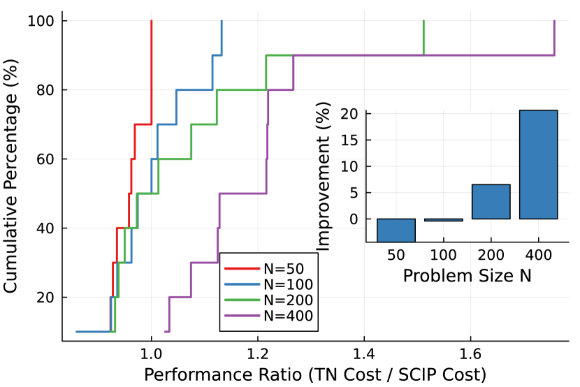
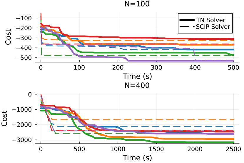
Figure 13: Performance comparison of our TN solver vs. SCIP on quadratic knapsack. (Left): Cumulative distribution of performance ratios (TN solver cost / SCIP cost), showcasing the percentage of instances where the TN algorithm outperforms SCIP (lower cost ratios indicate better performance). Inset corresponds to the average performance improvement of the TN solver over SCIP by problem size. The plot reveals that the TN solver consistently outperforms SCIP in larger problem instances ($N\geq 200$). (Right): Solver costs over time on five random problem realizations for problem sizes $N=100$, $N=400$.

VIII Conclusions and Outlook

In this work we have introduced a novel way of embedding arbitrary linear constraints into a tensor network using ideas from constraint programming and inspired by the theory of $U(1)$ symmetric tensor networks. While the connection between linear constraints and tensor networks is not new, see e.g. Biamonte et al. (2015); Kourtis et al. (2019); Liu et al. (2021); Hao et al. (2022); Ryzhakov and Oseledets (2022); Liu et al. (2023), our approach is not limited to local constraints, and scale well for reasonable constraints, including inequalities. Furthermore, we have introduced a new canonical form for constrained MPS and used it as part of an optimization algorithm, Algorithm 3, which is inspired by the GEO framework of Ref. Alcazar et al. (2024), and the constrained embedding and rebuild steps of Algorithm 1 of Ref. Lopez-Piqueres et al. (2022). The present approach is not limited to equality constraints, includes annealing in the selection of candidates, and the rebuild step is chosen judiciously based on the current samples’ costs.

Future work is directed both at applying some of these techniques to new domains, as well as on improving some of the steps developed here. The constraints discussed in this work are not just restricted to combinatorial optimization problems. One potential application of our constrained tensor network is precisely in the context of quantum many-body physics where the $U(1)$ global symmetry may be mildly broken. A classic example of $U(1)$ conservation is magnetization in spin chains: $\sum_{i}\hat{S}_{i}^{z}=M$, where $\hat{S}_{i}^{z}$ corresponds to the local magnetization of spin $i$ along the $z$ direction, with eigenvalues $s_{i}^{z}\in\{-1/2,1/2\}$. Such conservation laws, while physically motivated, are often an idealization. Various sources of noise in an experimental system can break, even if only mildly, such conservation laws. A relevant question in this context is under which setups one would have $M_{l}\leq\sum_{i}\hat{S}_{i}^{z}\leq M_{u}$, where $M_{l/u}$ are some fixed lower/upper bounds to the total magnetization. Such constraints could be easily handled by our tensor network approach.

Further improvements of this work involve better handling of multiple constraints. The scaling for this seems to be exponential in the number of constraints, by means of analyzing the facility location problem. Potential workarounds to this curse of constraints include constructing an ensemble of $M$ constrained MPS each handling a separate constraint and judiciously optimizing the ensemble (e.g. during the optimization process certain blocks on each MPS may disappear, which would make the composition of MPS easier upon optimizing). Relatedly, finding ways to extract QRegion blocks from data, similar to the way one can extract quantum numbers from data as proposed in Ref. Lopez-Piqueres et al. (2022), would certainly be a way to ameliorate the bottlenecks from embedding all the constraints exactly.

Appendix A Proof of optimal factorization

In this section, we will solve the optimal factorization in Eq. 11.

$$\text{min}_{\bar{U}_{i},\bar{F}}(\left\|W-\bar{U}\bar{F}\right\|^{2})\quad\text{s.t.}\quad\bar{U}^{\dagger}_{i}\bar{U}_{i}=I_{i}\quad\forall i$$ (31)

Due to the isometry constraint, we add Lagrange multipliers $\bar{\Lambda}_{i}$ into the target function $f\left(\bar{U}_{i},\bar{F}\right)$

$$f\left(\bar{U}_{i},\bar{F}\right) = \text{Tr}\left((W-\bar{U}\bar{F})(W-\bar{U}\bar{F})^{\dagger}\right)+\text{Tr}\left(\bar{\Lambda}_{i}(\bar{U}^{\dagger}_{i}\bar{U}_{i}-I_{i})\right)$$ (32)

In general, the Lagrange multipliers should be symmetric matrix. Since any unitary rotations in the subspace spanned by columns of $\bar{U}_{i}$ are equivalent. We choose the rotation so that the multiplers are diagonalized and represent by $\bar{\Lambda}_{i}$.

$$f\left(\bar{U}_{i},\bar{F}\right) = \text{Tr}\left(WW^{\dagger}-\bar{U}\bar{F}W^{\dagger}-W\bar{F}^{\dagger}\bar{U}^{\dagger}+\bar{U}\bar{F}\bar{F}^{\dagger}\bar{U}^{\dagger}\right)+\text{Tr}\left(\bar{\Lambda}_{i}(\bar{U}^{\dagger}_{i}\bar{U}_{i}-I_{i})\right)$$ (33)

$$= \text{Tr}\left(WW^{\dagger}-\bar{U}\bar{F}W^{\dagger}-W\bar{F}^{\dagger}\bar{U}^{\dagger}+\bar{F}\bar{F}^{\dagger}\bar{U}^{\dagger}\bar{U}\right)+\text{Tr}\left(\bar{\Lambda}_{i}(\bar{U}^{\dagger}_{i}\bar{U}_{i}-I_{i})\right)$$ (34)

$$= \text{Tr}\left(WW^{\dagger}-\bar{U}\bar{F}W^{\dagger}-W\bar{F}^{\dagger}\bar{U}^{\dagger}+\bar{F}\bar{F}^{\dagger}\right)+\text{Tr}\left(\bar{\Lambda}_{i}(\bar{U}^{\dagger}_{i}\bar{U}_{i}-I_{i})\right)$$ (35)

The second equal sign holds due to cyclic identity in the trace. The third equal sign holds due to the isometry constrain of $\bar{U}$. We can then split $\bar{U}=\oplus_{i}\bar{U}_{i}$ and insert identity $\bar{U}=\sum_{i}P_{i}\bar{U}P_{i}=\oplus_{i}\bar{U}_{i}$ and $\sum_{i}P_{i}=I$ into the loss.

$$f\left(\bar{U}_{i},\bar{F}\right) = \text{Tr}\left(WW^{\dagger}-\bar{U}\bar{F}W^{\dagger}-W\bar{F}^{\dagger}\bar{U}^{\dagger}+\bar{F}\bar{F}^{\dagger}\right)+\text{Tr}\left(\bar{\Lambda}_{i}(\bar{U}^{\dagger}_{i}\bar{U}_{i}-I_{i})\right)$$ (36)

$$= \text{Tr}\left(WW^{\dagger}-\sum_{i}P_{i}\bar{U}P_{i}\bar{F}W^{\dagger}-W\bar{F}^{\dagger}\sum_{i}P_{i}\bar{U}^{\dagger}P_{i}+\sum_{i}P_{i}\bar{F}\bar{F}^{\dagger}P_{i}\right)+\text{Tr}\left(\bar{\Lambda}_{i}(\bar{U}^{\dagger}_{i}\bar{U}_{i}-I_{i})\right)$$ (37)

where $P_{i}$ is the projector into subspace defined by row index block structure.

$$f\left(\bar{U}_{i},\bar{F}\right) = \text{Tr}\left(WW^{\dagger}-\sum_{i}\bar{U_{i}}\bar{F}_{i}W_{i}^{\dagger}-\sum_{i}W_{i}\bar{F}_{i}^{\dagger}\bar{U}_{i}^{\dagger}+\sum_{i}\bar{F_{i}}\bar{F_{i}}^{\dagger}\right)+\text{Tr}\left(\bar{\Lambda}_{i}(\bar{U}^{\dagger}_{i}\bar{U}_{i}-I_{i})\right)$$ (38)

where $W_{i}=P_{i}W$ are the rows of $W$, and $F_{i}=P_{i}F$, are projected on $i$-th subspace. To minimize $f\left(\bar{U}_{i},\bar{F}\right)$, we require

$$\frac{\partial f}{\partial\bar{U}_{i}^{\dagger}} =-W_{i}\bar{F}^{\dagger}+\bar{U}_{i}\bar{\Lambda}_{i} =0$$ (39)

$$\frac{\partial f}{\partial\bar{F}_{i}^{\dagger}} =-\bar{U}_{i}^{\dagger}W_{i}+\bar{F}_{i} =0$$ (40)

From Eq. 40, we can get

$$\bar{F}_{i}=\bar{U}_{i}^{\dagger}W_{i}$$ (41)

when substitution into Eq. 39 we get

$$W_{i}W_{i}^{\dagger}\bar{U}_{i}=\bar{U}_{i}\bar{\Lambda}_{i}$$ (42)

This is the eigenvalue decomposition of $W_{i}W_{i}^{\dagger}$, which is equivalent to SVD decomposition of $W_{i}$. Suppose

$$W_{i}=U_{i}\Lambda_{i}V^{\dagger}_{i}$$

The symbols without bar means no truncation has been applied.

$$\bar{F}_{i} = \bar{U}_{i}^{\dagger}W_{i}$$ (43)

$$= \bar{U}_{i}U_{i}\Lambda_{i}V^{\dagger}_{i}$$ (44)

$$= \bar{\Lambda}_{i}\bar{V}^{\dagger}_{i}$$ (45)

The loss would be given by

$$\sum_{i}(\Lambda_{i}-\bar{\Lambda}_{i})^{2}$$

So the optimal truncation is selecting the largest $\chi$ values among all $\lambda_{i}^{j}$ values.

References

- Hastings (2006) M. B. Hastings, “Solving gapped hamiltonians locally,” Phys. Rev. B 73, 085115 (2006).
- Hastings (2007) Matthew B Hastings, “An area law for one-dimensional quantum systems,” Journal of statistical mechanics: theory and experiment 2007, P08024 (2007).
- Verstraete and Cirac (2004) Frank Verstraete and J Ignacio Cirac, “Renormalization algorithms for quantum-many body systems in two and higher dimensions,” arXiv preprint cond-mat/0407066 (2004).
- Perez-Garcia et al. (2007) David Perez-Garcia, Frank Verstraete, J Ignacio Cirac, and Michael M Wolf, “Peps as unique ground states of local hamiltonians,” arXiv preprint arXiv:0707.2260 (2007).
- Shi et al. (2006) Y-Y Shi, L-M Duan, and Guifre Vidal, “Classical simulation of quantum many-body systems with a tree tensor network,” Physical review a 74, 022320 (2006).
- Singh et al. (2011) Sukhwinder Singh, Robert N. C. Pfeifer, and Guifre Vidal, “Tensor network states and algorithms in the presence of a global u(1) symmetry,” Phys. Rev. B 83, 115125 (2011).
- Singh and Vidal (2012) Sukhwinder Singh and Guifre Vidal, “Tensor network states and algorithms in the presence of a global su(2) symmetry,” Phys. Rev. B 86, 195114 (2012).
- Weichselbaum (2012) Andreas Weichselbaum, “Non-abelian symmetries in tensor networks: A quantum symmetry space approach,” Annals of Physics 327, 2972–3047 (2012).
- Silvi et al. (2019) Pietro Silvi, Ferdinand Tschirsich, Matthias Gerster, Johannes Jünemann, Daniel Jaschke, Matteo Rizzi, and Simone Montangero, “The Tensor Networks Anthology: Simulation techniques for many-body quantum lattice systems,” SciPost Phys. Lect. Notes , 8 (2019).
- Lopez-Piqueres et al. (2022) Javier Lopez-Piqueres, Jing Chen, and Alejandro Perdomo-Ortiz, “Symmetric tensor networks for generative modeling and constrained combinatorial optimization,” Machine Learning: Science and Technology 4 (2022).
- Schollwöck (2011) Ulrich Schollwöck, “The density-matrix renormalization group in the age of matrix product states,” Annals of physics 326, 96–192 (2011).
- Han et al. (2018) Zhao-Yu Han, Jun Wang, Heng Fan, Lei Wang, and Pan Zhang, “Unsupervised generative modeling using matrix product states,” Physical Review X 8, 031012 (2018).
- Glover et al. (2019) Fred Glover, Gary Kochenberger, and Yu Du, “A tutorial on formulating and using qubo models,” (2019), arXiv:1811.11538 [cs.DS] .
- Alcazar et al. (2024) Javier Alcazar, Mohammad Ghazi Vakili, Can B Kalayci, and Alejandro Perdomo-Ortiz, “Enhancing combinatorial optimization with classical and quantum generative models,” Nature Communications 15, 2761 (2024).
- Ferris and Vidal (2012) Andrew J. Ferris and Guifre Vidal, “Perfect sampling with unitary tensor networks,” Phys. Rev. B 85, 165146 (2012).
- Bestuzheva et al. (2023) Ksenia Bestuzheva, Antonia Chmiela, Benjamin Müller, Felipe Serrano, Stefan Vigerske, and Fabian Wegscheider, “Global optimization of mixed-integer nonlinear programs with scip 8,” Journal of Global Optimization , 1–24 (2023).
- Lubin et al. (2023) Miles Lubin, Oscar Dowson, Joaquim Dias Garcia, Joey Huchette, Benoît Legat, and Juan Pablo Vielma, “Jump 1.0: Recent improvements to a modeling language for mathematical optimization,” Mathematical Programming Computation 15, 581–589 (2023).
- Fishman et al. (2022) Matthew Fishman, Steven R. White, and E. Miles Stoudenmire, “Codebase release 0.3 for ITensor,” SciPost Phys. Codebases , 4–r0.3 (2022).
- (19) https://github.com/JaviLoPiq/ConstrainTNet.jl.git.
- Biamonte et al. (2015) Jacob D Biamonte, Jason Morton, and Jacob Turner, “Tensor network contractions for# sat,” Journal of Statistical Physics 160, 1389–1404 (2015).
- Kourtis et al. (2019) Stefanos Kourtis, Claudio Chamon, Eduardo R. Mucciolo, and Andrei E. Ruckenstein, “Fast counting with tensor networks,” SciPost Phys. 7, 060 (2019).
- Liu et al. (2021) Jin-Guo Liu, Lei Wang, and Pan Zhang, “Tropical tensor network for ground states of spin glasses,” Phys. Rev. Lett. 126, 090506 (2021).
- Hao et al. (2022) Tianyi Hao, Xuxin Huang, Chunjing Jia, and Cheng Peng, “A quantum-inspired tensor network algorithm for constrained combinatorial optimization problems,” Frontiers in Physics 10, 906590 (2022).
- Ryzhakov and Oseledets (2022) Gleb Ryzhakov and Ivan Oseledets, “Constructive tt-representation of the tensors given as index interaction functions with applications,” (2022), arXiv:2206.03832 [math.NA] .
- Liu et al. (2023) Jin-Guo Liu, Xun Gao, Madelyn Cain, Mikhail D Lukin, and Sheng-Tao Wang, “Computing solution space properties of combinatorial optimization problems via generic tensor networks,” SIAM Journal on Scientific Computing 45, A1239–A1270 (2023).