Nonparametric Inference on Dose-Response Curves Without the Positivity Condition

Supplement to “Nonparametric Inference on Dose-Response Curves Without the Positivity Condition”

Abstract

Existing statistical methods in causal inference often rely on the assumption that every individual has some chance of receiving any treatment level regardless of its associated covariates, which is known as the positivity condition. This assumption could be violated in observational studies with continuous treatments. In this paper, we present a novel integral estimator of the causal effects with continuous treatments (i.e., dose-response curves) without requiring the positivity condition. Our approach involves estimating the derivative function of the treatment effect on each observed data sample and integrating it to the treatment level of interest so as to address the bias resulting from the lack of positivity condition. The validity of our approach relies on an alternative weaker assumption that can be satisfied by additive confounding models. We provide a fast and reliable numerical recipe for computing our estimator in practice and derive its related asymptotic theory. To conduct valid inference on the dose-response curve and its derivative, we propose using the nonparametric bootstrap and establish its consistency. The practical performances of our proposed estimators are validated through simulation studies and an analysis of the effect of air pollution exposure (PM_2.5) on cardiovascular mortality rates.

, and

1 Introduction

In observational studies, the causal effect of interest does not always result from a standard binary intervention but rather comes as a consequence of a continuous treatment or exposure. Such a causal effect on the outcome variable $Y\in\mathcal{Y}\subset\mathbb{R}$ from a continuous treatment variable $T\in\mathcal{T}\subset\mathbb{R}$ is known as the (causal) dose-response curve or relationship due to its major application in studying biological effects (Waud, 1975). More precisely, a dose-response curve characterizes the average outcome if all units would have been assigned to a certain treatment level $T=t$. In practice, it is fairly common that an additional set of covariates $\bm{S}\in\mathcal{S}\subset\mathbb{R}^{d}$ is collected, which, to some extent, contains all the possible confounding variables that influence both the treatment $T$ and the outcome $Y$. Under regularity conditions (see Section 2.2), the dose-response curve coincides with the so-called covariate-adjusted regression function $t\mapsto m(t)=\mathbb{E}\left[\mu(t,\bm{S})\right]$ with $\mu(t,\bm{s})=\mathbb{E}\left(Y|T=t,\bm{S}=\bm{s}\right)$ and is thus identifiable from the observed data $\left\{(Y_{i},T_{i},\bm{S}_{i})\right\}_{i=1}^{n}$ for any $t\in\mathcal{T}$ (Robins et al., 2000; Neugebauer and van der Laan, 2007; Díaz and van der Laan, 2013; Kennedy et al., 2017). Alternatively, the covariate-adjusted regression function $m(t)$ can be viewed as a univariate summary function of the outcome against a continuous covariate $T$ when we average the regression function $\mu(t,\bm{s})$ over all other covariates $\bm{S}$ (Takatsu and Westling, 2022).

However, the regularity conditions for identifying and estimating the dose-response curve might not be verifiable or could even be violated in observational studies. In particular, it is commonly assumed that there is a sufficient amount of variability in the treatment assignment within each strata of the covariates, which is captured by the following positivity or overlapping condition.

Assumption A0 (Positivity).

The conditional density $p(t|\bm{s})$ is bounded above and away from zero almost surely for all $t\in\mathcal{T}$ and $\bm{s}\in\mathcal{S}$.

The positivity condition (A0) may be violated in observational studies for either of the following two reasons: (i) theoretically, it is impossible for some individuals with certain covariate values to receive some levels of the treatment, and (ii) practically, individuals at some levels of the treatment may not be collected in the finite data sample; see Cole and Hernán (2008); Westreich and Cole (2010); Petersen et al. (2012) for related discussions. These problems are particularly pervasive under the context of continuous treatments. For instance, air pollution levels can vary greatly across larger regions but remain relatively consistent within smaller and nearby areas. Therefore, individuals at the same location are typically only get exposed to one level of air pollution, i.e., spatial confounding variables may change at a finer scale than the variation of exposure, thereby violating the positivity condition (Paciorek, 2010; Schnell and Papadogeorgou, 2020; Keller and Szpiro, 2020). As a more concrete example, consider a single confounder model

$$Y=T^{2}+T+1+10S+\epsilon,\quad T=\sin(\pi S)+E,\quad\text{ and }\quad S\sim\text{Uniform}[-1,1]\subset\mathbb{R},$$ (1)

where $E\sim\text{Uniform}[-0.3,0.3]$ is an independent treatment variation and $\epsilon\sim\mathcal{N}(0,1)$ is an exogenous normal noise. The marginal supports of $T$ and $S$ are $\mathcal{T}=[-1.3,1.3]$ and $\mathcal{S}=[-1,1]$ respectively, while the joint support of $(T,S)$ only covers a thin band region of the product space $\mathcal{T}\times\mathcal{S}$; see the left panel of Fig 1. The conditional density $p(t|s)$ for any $s\in\mathcal{S}$ is 0 within the gray regions, and the positivity condition (A0) clearly fails. Without (A0), the existing approaches for estimating the dose-response curve $m(t)$ and its derivative $\theta(t)=m^{\prime}(t)$ can be very unstable at some specific treatment levels; see the usual regression adjustment estimators (defined in (6) and Remark 1 below) in the middle and right panels of Fig 1 for illustrations.

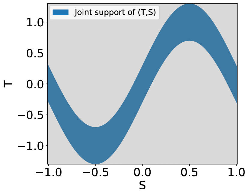
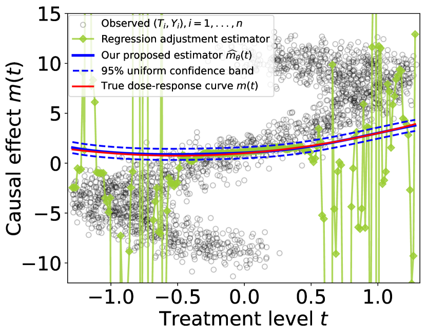
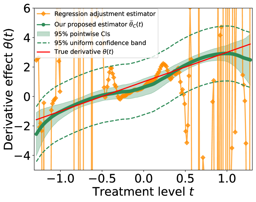
Figure 1: Simulation results under the single confounder model (1). Left: The support of the joint distribution of $(T,S)$. Middle: The estimated dose-response curves by usual regression adjustment and our proposed estimators overlain with the true one $m(t)$. Right: The estimated derivatives of the dose-response curve by usual regression adjustment and our proposed estimators overlain with the true one $\theta(t)$. The middle and right panels also present the 95% confidence intervals and/or uniform confidence bands from our proposed estimators as shaded regions and dashed lines, respectively.

In this paper, we propose a novel integral estimator that can consistently recover the entire dose-response curve $m(t)$ and a localized estimator of its derivative $\theta(t)=m^{\prime}(t)$ even when the positivity condition (A0) fails to hold in some regions of the product space $\mathcal{T}\times\mathcal{S}$; see the middle and right panels of Fig 1. Our main contributions are summarized as follows:

1. Methodology: After discussing the identification conditions of $m(t)$ as a causal dose-response curve in Section 2, we introduce our integral estimator of $m(t)$ in Section 3.1, which is constructed from a localized estimator of $\theta(t)$ around the observed data and extrapolate to any treatment level $t\in\mathcal{T}$ through the fundamental theorem of calculus. Such an integral estimator can also be efficiently computed in practice via the Riemann sum approximation in Section 3.2 and be reliably inferred through nonparametric bootstrap in Section 3.3.

2. Asymptotic Theory: We establish uniform consistencies of our proposed integral estimator and localized derivative estimator under the context of kernel smoothing methods in Section 4.2. We also prove the validity of nonparametric bootstrap inference in Section 4.3.

3. Experiments: We demonstrate the finite-sample performances of our proposed estimators through simulation studies and a case study of the effect of fine particulate matter (PM_2.5) on cardiovascular mortality rates in Section 5. All the code for our experiments is available at https://github.com/zhangyk8/NPDoseResponse/tree/main/Paper_Code.

1.1 Other Related Works

Estimating the dose-response curve $m(t)$ is a technically difficult problem in causal inference due to the fact that $m(t)$ is not pathwise differentiable and cannot be consistently estimated in a $\sqrt{n}$ rate (Chamberlain, 1986; van der Vaart, 1991). Parametrically, Robins et al. (2000) pioneered a marginal structural model to estimate $m(t)$, whose dependence on the correct specification of a parametric model was later relaxed by van der Laan and Robins (2003); Neugebauer and van der Laan (2007) through a projection of $m(t)$ to the parametric model space. Nonparametrically, a regression adjustment approach to estimating $m(t)=\mathbb{E}\left[\mu(t,\bm{S})\right]$ under a two-stage kernel smoothing estimator was first studied by Newey (1994) and later adapted to the estimation of dose-response curves by Flores (2007). However, the consistency and asymptotic normality of their kernel-based estimators rely on an undersmoothing bandwidth, which is asymptotically smaller than the one that attains the optimal asymptotic bias-variance trade-off and is difficult to select in practice; see Section 5.7 in Wasserman (2006). On the contrary, our proposed integral estimator of $m(t)$ under the context of kernel smoothing is based on the derivative estimation and require neither explicit undersmoothing nor bias correction (Calonico et al., 2018; Takatsu and Westling, 2022), permitting the use of any bandwidth selection method in nonparametric regression.

There are many existing works about the estimation of average derivative effects in the literature; see Härdle and Stoker (1989); Powell et al. (1989); Newey and Stoker (1993); Cattaneo et al. (2010); Hirshberg and Wager (2020) and references therein. Under some regularity conditions, average derivative effects are identical to the so-called incremental treatment effects, which are closely related to the derivatives $\theta(t)=m^{\prime}(t)$ of dose-response curves; see Proposition 1 in Rothenhäusler and Yu (2019) and Section 6.1 in Hines et al. (2023).

All the aforementioned methods for estimating $m(t)$ and $\theta(t)$ assume the positivity condition (A0). Under the context of binary treatments, there are previous researches studying the dependence of common estimators on (A0) from the perspectives of convergence rates (Khan and Tamer, 2010; D’Amour et al., 2021) and empirical performances (Busso et al., 2014; Léger et al., 2022). To address the violation of positivity, some approaches considered trimming the extreme values of (estimated) propensity scores (i.e., discrete versions of the conditional density $p(t|\bm{s})$; Dehejia and Wahba 1999; Crump et al. 2009; Yang and Ding 2018), while others proposed robust estimation methods against the violation (Rothe, 2017; Ma and Wang, 2020). In addition, Kennedy (2019) considered switching the causal estimand to the incremental treatment effect for discrete treatments, which can be nonparametrically estimated without positivity. Rothenhäusler and Yu (2019) later studied the same estimand for continuous treatments. To the best of our knowledge, none of existing works address the nonparametric inference on $m(t)$ and $\theta(t)$ without assuming (A0).

1.2 Notations

Throughout the paper, we consider a real-valued outcome variable $Y\in\mathcal{Y}\subset\mathbb{R}$, univariate continuous treatment $T\in\mathcal{T}\subset\mathbb{R}$, and a vector of covariates $\bm{S}=(S_{1},...,S_{d})\in\mathcal{S}\subset\mathbb{R}^{d}$ with a fixed dimension $d$. We write $Y{\perp\!\!\!\perp}X$ when the random variables $Y,X$ are independent. The data sample consists of independent and identically distributed (i.i.d.) observations $\bm{U}_{i}=(Y_{i},T_{i},\bm{S}_{i}),i=1,...,n$ with the common distribution $\mathrm{P}$ and Lebesgue density $p(y,t,\bm{s})=p(y|t,\bm{s})\cdot p(t|\bm{s})\cdot p_{S}(\bm{s})$. Here, $p_{T}(t)$ and $p_{S}(\bm{s})$ are the marginal densities of $T$ and $\bm{S}$, respectively, and $p(t|\bm{s})=\frac{\partial}{\partial t}\mbox{$\mathrm{P}$}\left(T\leq t|\bm{S}=\bm{s}\right)$ is the conditional density of $T$ given covariates $\bm{S}=\bm{s}$. We also denote the joint density of $(T,\bm{S})$ by $p(t,\bm{s})=p(t|\bm{s})\cdot p_{S}(\bm{s})=p(\bm{s}|t)\cdot p_{T}(t)$. Let $\mathbb{P}_{n}$ be the empirical distribution of the observed data so that $\mathbb{P}_{n}g=\int g(\bm{u})\,d\mathbb{P}_{n}(\bm{u})=\frac{1}{n}\sum_{i=1}^{n}g(\bm{U}_{i})$ for some measurable function $g$. At the population level, we denote $\mbox{$\mathrm{P}$}g=\mathbb{E}\left[g(\bm{U})\right]=\int g(\bm{u})\,d\mbox{$\mathrm{P}$}(\bm{u})$ for $\mathrm{P}$-integrable function $g$. In addition, we define the empirical process evaluated at a $\mathrm{P}$-integrable function $g$ as $\mathbb{G}_{n}(g)=\sqrt{n}\left(\mathbb{P}_{n}-\mbox{$\mathrm{P}$}\right)g=\frac{1}{\sqrt{n}}\sum_{i=1}^{n}\left[g(\bm{U}_{i})-\mathbb{E}\left(g(\bm{U}_{i})\right)\right]$. Finally, we use $\mathbbm{1}_{A}$ to denote the indicator function of a set $A$.

We use the big-$O$ notation $h_{n}=O(g_{n})$ if $|h_{n}|$ is upper bounded by a positive constant multiple of $g_{n}>0$ when $n$ is sufficiently large. In contrast, $h_{n}=o(g_{n})$ when $\lim_{n\to\infty}\frac{|h_{n}|}{g_{n}}=0$. For random variables, the notation $o_{P}(1)$ is short for a sequence of random variables converging to zero in probability, while the expression $O_{P}(1)$ denotes the sequence that is bounded in probability. We also use the notation $a_{n}\lesssim b_{n}$ or $b_{n}\gtrsim a_{n}$ when there exists an absolute constant $A>0$ such that $a_{n}\leq Ab_{n}$ when $n$ is large. If $a_{n}\gtrsim b_{n}$ and $a_{n}\lesssim b_{n}$, then $a_{n},b_{n}$ are asymptotically equal and it is denoted by $a_{n}\asymp b_{n}$.

2 Model Setups and Identification Conditions

We assume that $\bm{U}_{i}=(Y_{i},T_{i},\bm{S}_{i}),i=1,...,n$ are i.i.d. observations generated from the following model:

$$\begin{split}Y&=\mu(T,\bm{S})+\epsilon\quad\text{ and }\quad T=f(\bm{S})+E,\end{split}$$ (2)

where $E\in\mathbb{R}$ is the treatment variation with $\mathbb{E}(E)=0$, $E{\perp\!\!\!\perp}\bm{S}$, and $\epsilon\in\mathbb{R}$ is an exogenous noise variable with $\epsilon{\perp\!\!\!\perp}E,\epsilon{\perp\!\!\!\perp}\bm{S}$ and $\mathbb{E}(\epsilon)=0,\mathrm{Var}(\epsilon)=\sigma^{2}>0,\mathbb{E}(\epsilon^{4})<\infty$. The function $f$ determines how the covariates (or confounding variables) $\bm{S}$ influence the treatment $T$. Under model (2), the covariate-adjusted regression function (or the dose-response curve under identification conditions in Section 2.2) is given by

$$t\mapsto m(t)=\mathbb{E}\left[\mathbb{E}(Y|T=t,\bm{S})\right]=\mathbb{E}\left[\mu(t,\bm{S})\right],$$

and its derivative is written as $\theta(t)=m^{\prime}(t)=\frac{d}{dt}\mathbb{E}\left[\mu(t,\bm{S})\right]$. Notice that the derivative function $\theta(t)$ can be viewed as the continuous version of the average treatment effect in causal inference. In the presence of confounding variables $\bm{S}$, $m(t)$ cannot be identified by regressing $Y$ only with respect to $T$, because $m(t)=\mathbb{E}\left[\mu(t,\bm{S})\right]\neq\mathbb{E}\left(Y|T=t\right)=\mathbb{E}\left[\mu(T,\bm{S})|T=t\right]$.

2.1 Motivating Example: Additive Confounding Model

One important exemplification of model (2) that we will frequently refer to in this paper is the following additive confounding model:

$$\begin{split}Y&=\bar{m}(T)+\eta(\bm{S})+\epsilon\quad\text{ and }\quad T=f(\bm{S})+E,\end{split}$$ (3)

where $\bar{m}(t)$ is the primary treatment effect of interest and $\eta(\bm{s})$ is the random effect with $\mbox{$\mathbb{E}$}\left[\eta(\bm{S})\right]=0$. Such an additive form is a common working model in spatial confounding problems (Paciorek, 2010; Schnell and Papadogeorgou, 2020) and also known as the geoadditive structural equation model (Kammann and Wand, 2003; Thaden and Kneib, 2018; Wiecha and Reich, 2024), where $\bm{S}\in\mathbb{R}^{d}$ are the spatial locations (usually with $d=2$) or other spatially correlated covariates that affect both the treatment $T$ and the outcome $Y$. We summarize key properties of the additive confounding model (3) in the following proposition.

Proposition 1 (Properties of the additive confounding model (3)).

Let $\theta_{M}(t)=\mathbb{E}\left[\frac{\partial}{\partial t}\mu(t,\bm{S})\right]$ and $\theta_{C}(t)=\mathbb{E}\left[\frac{\partial}{\partial t}\mu(t,\bm{S})\big{|}T=t\right]$, where $\mu(t,\bm{s})=\mathbb{E}\left[Y|T=t,\bm{S}=\bm{s}\right]$. Under the additive confounding model (3) with $\mbox{$\mathbb{E}$}\left[\eta(\bm{S})\right]=0$, the following results hold for all $t\in\mathcal{T}$:

1. $m(t)=\bar{m}(t)$.

2. $m(t)\neq\mbox{$\mathbb{E}$}(Y|T=t)=\bar{m}(t)+\mbox{$\mathbb{E}$}\left[\eta(\bm{S})|T=t\right]$ when $\mbox{$\mathbb{E}$}\left[\eta(\bm{S})|T=t\right]\neq 0$.

3. $\theta(t)=\theta_{M}(t)=\theta_{C}(t)$.

4. $\theta(t)\neq\frac{d}{dt}\mbox{$\mathbb{E}$}\left[\mu(t,\bm{S})|T=t\right]=\theta(t)+\frac{d}{dt}\mbox{$\mathbb{E}$}\left[\eta(\bm{S})|T=t\right]$ when $\frac{d}{dt}\mbox{$\mathbb{E}$}\left[\eta(\bm{S})|T=t\right]\neq 0$.

5. $\mathbb{E}\left[\mu(T,\bm{S})\right]=\mathbb{E}\left[m(T)\right]$ even when $\mbox{$\mathbb{E}$}\left[\eta(\bm{S})\right]\neq 0$.

The above results hold even if the treatment variation $E=0$ almost surely.

The proof of Proposition 1 is in Section B.1. Note that in Proposition 1(e), the first expectation is taken with respect to the joint distribution of $(T,\bm{S})$ while the second expectation is taken with respect to the marginal distribution of $T$.

2.2 Identification Conditions

While $m(t)$ can be defined through model (2), we need some additional assumptions in order to express $m(t)$ as a causal effect of $T$ on $Y$ and identify it from the observed data $\left\{(Y_{i},T_{i},\bm{S}_{i})\right\}_{i=1}^{n}$. Following the potential outcome framework (Rubin, 1974), we let $Y(t,\bm{s})$ denote the potential outcome that would have been observed under treatment level $T=t$ and covariate vector $\bm{S}=\bm{s}$. We summarize the required assumptions as follows.

Assumption A1 (Identification conditions for $m(t)$).

1. (Treatment effect and consistency) $Y(t,\bm{s})=Y(t)=Y$ for any $t\in\mathcal{T}$ and $\bm{s}\in\mathcal{S}$.

2. (Ignorability or unconfoundingness) $Y(t){\perp\!\!\!\perp}T\,\big{|}\,\bm{S}$ for all $t\in\mathcal{T}$.

3. (Treatment variation) The treatment variation $E$ has nonzero variance, i.e., $\mathrm{Var}(E)>0$.

Assumption A1(a) is a continuous version of the stable unit treatment value assumption (SUTVA; Page 19 of Cox 1958 and Rubin 1980). The first equality ensures that the potential outcome $Y(t)$ under treatment level $T=t$ is well-defined whatever value the covariate vector $\bm{S}$ takes, while the second equality guarantees that the treatment level of any subject does not affect the potential outcomes of others (i.e., no interference) and there are no different versions of treatments. Given that both the treatment $T$ and the outcome $Y$ are continuous, the essential consistency condition that we need is the identity of conditional distributions $\mbox{$\mathrm{P}$}\left(Y(T)\leq y|T=t\right)=\mbox{$\mathrm{P}$}\left(Y(t)\leq|T=t\right)$ for any $t\in\mathcal{T}$ and $y\in\mathcal{Y}$; see Gill and Robins (2001) for details. The ignorability condition (Assumption A1(b)) was first generalized to continuous treatments by Hirano and Imbens (2004), stating that the potential outcome variable is independent of the treatment level within any specific strata of covariates. In the context of spatial confounding, the ignorability condition holds when the spatial locations are taken into account (Gilbert et al., 2023). It also implies that the mean potential outcome under $T=t$ remains the same across all treatment levels when we condition on $\bm{S}=\bm{s}$. Finally, the treatment variation condition (Assumption A1(c)) is crucial for identifying the conditional mean outcome (or regression) function $\mu(t,\bm{s})$ on a non-degenerate region of $\mathcal{T}\times\mathcal{S}$. When $\mathrm{Var}(E)=0$, $\mu(t,\bm{s})$ can only be identified on the lower dimensional surface $\left\{(t,\bm{s})\in\mathcal{T}\times\mathcal{S}:t=f(\bm{s})\right\}$, which is also the support of $(T,\bm{S})$. We derive nonparametric bounds on $m(t)=\mbox{$\mathbb{E}$}\left[\mu(t,\bm{S})\right]$ and its derivative $\theta(t)=\frac{d}{dt}\mbox{$\mathbb{E}$}\left[\mu(t,\bm{S})\right]$ in Section A. We also demonstrate how $\mathrm{Var}(E)=0$ can lead to ambiguous definitions of the associated dose-response curves in Example 1 below.

Example 1 (Necessity of $\mathrm{Var}(E)>0$).

Suppose that $\mathrm{Var}(E)=0$ and $T=f(\bm{S})+E=S_{1}$ almost surely, where $S_{1}$ is the first component of $\bm{S}\in\mathcal{S}\subset\mathbb{R}^{d}$. We further assume that $\mathbb{E}(S_{1})=0$. Now, consider two equivalent conditional mean outcome functions

$$\mu_{1}(T,\bm{S})\equiv T+2S_{1}\quad\text{ and }\quad\mu_{2}(T,\bm{S})\equiv 2T+S_{1},$$

both of which are equal to $3S_{1}$ and agree on the support $\left\{(t,\bm{s})\in\mathcal{T}\times\mathcal{S}:t=f(\bm{s})=s_{1}\right\}$. However, these two conditional mean outcome functions lead to two distinct treatment effects:

$$m_{1}(t)=\mbox{$\mathbb{E}$}\left[\mu_{1}(t,\bm{S})\right]=t\quad\text{ and }\quad m_{2}(t)=\mbox{$\mathbb{E}$}\left[\mu_{2}(t,\bm{S})\right]=2t,$$

whose derivatives are different as well.

Under Assumption A1, the dose-response curve $t\mapsto\mbox{$\mathbb{E}$}\left[Y(t)\right]$ is identical to the standard covariate-adjusted regression function $m(t)=\mbox{$\mathbb{E}$}\left[\mu(t,\bm{S})\right]=\int_{\mathcal{S}}\mu(t,\bm{s})\cdot p_{S}(\bm{s})\,d\bm{s}$ and can thus be estimated from the observed data $\left\{(Y_{i},T_{i},\bm{S}_{i})\right\}_{i=1}^{n}$. To estimate the derivative $\theta(t)=m^{\prime}(t)=\frac{d}{dt}\mbox{$\mathbb{E}$}\left[\mu(t,\bm{S})\right]$ of the dose-response curve from the observed data sample, we impose an additional assumption on the conditional mean outcome function $\mu(t,\bm{s})=\mbox{$\mathbb{E}$}(Y|T=t,\bm{S}=\bm{s})$ that enables us to bypass the positivity condition (A0).

Assumption A2 (Identification condition for $\theta(t)$).

The function $\mu(t,\bm{s})$ is continuously differentiable with respect to $t$ for any $(t,\bm{s})\in\mathcal{T}\times\mathcal{S}$ and the following two equalities hold true:

$$\theta(t)=\mbox{$\mathbb{E}$}\left[\frac{\partial}{\partial t}\mu(t,\bm{S})\right]=\mbox{$\mathbb{E}$}\left[\frac{\partial}{\partial t}\mu(t,\bm{S})\Big{|}T=t\right]$$ (4)

and

$$\mathbb{E}\left[\mu(T,\bm{S})\right]=\mathbb{E}\left[m(T)\right].$$ (5)

The first equality in (4) is a mild condition and can be satisfied under various settings. In particular, it holds when $\left|\frac{\partial}{\partial t}\mu(t,\bm{S})\right|$ is bounded by an integrable function $\bar{\mu}(\bm{S})$ with respect to the distribution of $\bm{S}$; see Theorem 1.1 and Example 1.8 in Shao (2003). The second equality in (4) as well as the equation (5) of Assumption A2 are stricter but still valid under the additive confounding model in Section 2.1; recall Proposition 1(c,e). Under Assumption A2, we can express $\theta(t)$ in three different but also equivalent ways

$$\theta(t)=\underbrace{\frac{d}{dt}\mathbb{E}\left[\mu(t,\bm{S})\right]}_{m^{\prime}(t)}=\underbrace{\mbox{$\mathbb{E}$}\left[\frac{\partial}{\partial t}\mu(t,\bm{S})\right]}_{\theta_{M}(t)}=\underbrace{\mbox{$\mathbb{E}$}\left[\frac{\partial}{\partial t}\mu(t,\bm{S})\Big{|}T=t\right]}_{\theta_{C}(t)}.$$

Estimating the derivative effect $\theta(t)$ through the form of $\theta_{C}(t)$ is our key technique to bypass the particularly strong positivity condition (A0) under the continuous treatment setting. After $\theta(t)$ is consistently recovered, we refer the estimation back to the dose-response curve $m(t)$ by (5) and the fundamental theorem of calculus; see Section 3.1 for details.

3 Nonparametric Inference Without the Positivity Condition

Under the positivity condition (A0), together with Assumption A1, the dose-response curve $m(t)=\mbox{$\mathbb{E}$}\left[Y(t)\right]$ can be identified through the covariate-adjusted regression function $\mbox{$\mathbb{E}$}\left[\mu(t,\bm{S})\right]$ from the observed data $\left\{(Y_{i},T_{i},\bm{S}_{i})\right\}_{i=1}^{n}$, suggesting the following regression adjustment (RA) or G-computation (Robins, 1986; Gill and Robins, 2001) estimator as:

$$\widehat{m}_{RA}(t)=\frac{1}{n}\sum_{i=1}^{n}\widehat{\mu}(t,\bm{S}_{i}),$$ (6)

where $\widehat{\mu}(t,\bm{s})$ is any consistent estimator of the conditional mean outcome function $\mu(t,\bm{s})$. However, when the positivity condition (A0) does not hold for some region in $\mathcal{T}\times\mathcal{S}$, the above estimator (6) will be unstable and even inconsistent. This is because without (A0), the joint density $p(t,\bm{S}_{i})=p(t|\bm{S}_{i})\cdot p_{S}(\bm{S}_{i})$ can be close to 0 for some $i=1,...,n$, and $\mu(t,\bm{s})$ cannot be consistently estimated for those query points $(t,\bm{S}_{i}),i=1,...,n$. Other existing methods for estimating $m(t)$, such as the inverse probability of treatment weighted (IPTW) or its augmented variants, also relies on the validity of (A0) for their consistency and empirical behaviors (Díaz and van der Laan, 2013; Kennedy et al., 2017; Huber et al., 2020; Colangelo and Lee, 2020). The same issue incurred by the failure of (A0) also applies to the estimation of $\theta(t)=m^{\prime}(t)$.

In this section, we introduce a novel integral estimator to resolve the inconsistency issues of existing estimators in recovering the dose-response curve $m(t)$ and its derivative $\theta(t)$ without the positivity condition (A0). On one hand, the estimation of $\theta(t)$ is based on the conditional expectation $\theta_{C}(t)\equiv\mbox{$\mathbb{E}$}\left[\frac{\partial}{\partial t}\mu(t,\bm{S})\Big{|}T=t\right]$ in (4), which only relies on the consistent estimation of $\frac{\partial}{\partial t}\mu(t,\bm{s})$ in the high density region of $p(\bm{s}|t)$. On the other hand, our proposed estimator of $m(t)$ generalizes the regression adjustment estimator (6) but remains consistent and numerically stable even when the conditional density $p(t|\bm{s})$ is zero for some values of $\bm{s}\in\mathcal{S}$ thanks to its integral formulation. We also provide a fast algorithm for computing our proposed estimator of $m(t)$ in practice and delineate the bootstrap inference procedures for both estimators of $\theta(t)$ and $m(t)$.

3.1 Proposed Integral Estimator of $m(t)$

Given the observed data $\left\{(Y_{i},T_{i},\bm{S}_{i})\right\}_{i=1}^{n}$, our proposal for removing the reliance of the positivity condition (A0) from (6) is based on three critical insights.

• Insight 1: Consistent estimation of $\mu(t,\bm{s})$ and $\frac{\partial}{\partial t}\mu(t,\bm{s})$ at each $(T_{i},\bm{S}_{i})$. Given that the observed data $(T_{i},\bm{S}_{i}),i=1,...,n$ generally appear in a high density region of $p(t,\bm{s})$, the conditional mean outcome function $\mu(t,\bm{s})$ can be well-estimated at each observation $(T_{i},\bm{S}_{i})$. As a result, one can expect that the partial derivative $\frac{\partial}{\partial t}\mu(t,\bm{s})$ can be consistently estimated at each observation $(T_{i},\bm{S}_{i})$ as well.

• Insight 2: Consistent estimation of $\theta(t)$ from a localized form $\theta_{C}(t)$. The equations (4) in Assumption A2 lead to two possible approaches to estimating the derivative effect $\theta(t)=\frac{d}{dt}\mathbb{E}\left[\mu(t,\bm{S})\right]$. One approach is via $\theta_{M}(t)=\mbox{$\mathbb{E}$}\left[\frac{\partial}{\partial t}\mu(t,\bm{S})\right]$, while the alternative is based on $\theta_{C}(t)=\mbox{$\mathbb{E}$}\left[\frac{\partial}{\partial t}\mu(t,\bm{S})\Big{|}T=t\right]$. Estimating $\theta(t)$ by $\theta_{C}(t)$ is preferable because $\theta_{M}(t)$ relies on a consistent estimator of $\frac{\partial}{\partial t}\mu(t,\bm{s})$ at each pair $(t,\bm{S}_{i})$, which is not possible when the positivity condition (A0) fails to hold at some $(t,\bm{S}_{i})$ for $i=1,...,n$. In contrast, the expression $\theta_{C}(t)$ only requires the estimator of $\frac{\partial}{\partial t}\mu(t,\bm{s})$ to be accurate at the covariate vector $\bm{s}$ with a high conditional density value $p(\bm{s}|t)$.

• Insight 3: Integral relation between $\theta(t)$ and $m(t)$. For any $t\in\mathcal{T}$, the fundamental theorem of calculus reveals that

  $$m(t)=m(T)+\int_{\widetilde{t}=T}^{\widetilde{t}=t}m^{\prime}(\widetilde{t})\,d\widetilde{t}=m(T)+\int_{\widetilde{t}=T}^{\widetilde{t}=t}\theta(\widetilde{t})\,d\widetilde{t}.$$

  Under Assumption A2, we take the expectation on both sides of the above equality to obtain that

  $$\begin{split}m(t)=\mbox{$\mathbb{E}$}\left[m(T)+\int_{\widetilde{t}=T}^{\widetilde{t}=t}\theta(\widetilde{t})\,d\widetilde{t}\right]&=\mbox{$\mathbb{E}$}\left[\mu(T,\bm{S})\right]+\mbox{$\mathbb{E}$}\left[\int_{\widetilde{t}=T}^{\widetilde{t}=t}\theta_{C}(\widetilde{t})\,d\widetilde{t}\right]\\ &=\mbox{$\mathbb{E}$}(Y)+\mbox{$\mathbb{E}$}\left\{\int_{\widetilde{t}=T}^{\widetilde{t}=t}\mbox{$\mathbb{E}$}\left[\frac{\partial}{\partial t}\mu(\widetilde{t},\bm{S})\Big{|}T=\widetilde{t}\right]\,d\widetilde{t}\right\}.\end{split}$$ (7)

  This expression suggests that as long as we have consistent estimators of $\mu(t,\bm{s})$ at $(T,\bm{S})$ and $\theta(t)$ near $T$, we can then use the integration to extrapolate the estimation to $\mu(t,\bm{S})$ and $m(t)$ for any $t\in\mathcal{T}$ even when $p(t,\bm{S})=0$.

According to the integral relation (7), we propose an integral estimator of the dose-response curve $m(t)$ as:

$$\widehat{m}_{\theta}(t)=\frac{1}{n}\sum_{i=1}^{n}\left[Y_{i}+\int_{\widetilde{t}=T_{i}}^{\widetilde{t}=t}\widehat{\theta}_{C}(\widetilde{t})\,d\widetilde{t}\right],$$ (8)

where $\widehat{\theta}_{C}(t)$ is a consistent estimator of $\theta_{C}(t)=\mbox{$\mathbb{E}$}\left[\frac{\partial}{\partial t}\mu(t,\bm{S})\Big{|}T=t\right]=\int\frac{\partial}{\partial t}\mu(t,\bm{s})\,d\mbox{$\mathrm{P}$}(\bm{s}|t)$. To construct an estimator of $\theta_{C}(t)$, we need to estimate two nuisance functions: (i) the partial derivative $\frac{\partial}{\partial t}\mu(t,\bm{s})$ of the conditional mean outcome function $\mu(t,\bm{s})$ and (ii) the conditional cumulative distribution function (CDF) $P(\bm{s}|t)$. In this paper, we leverage the following two kernel smoothing methods for estimating these two nuisance functions and leave other possibilities as a future direction.

3.1.1 Local Polynomial Regression Estimator of $\frac{\partial}{\partial t}\mu(t,\mathbf{s})$

We consider estimating $\frac{\partial}{\partial t}\mu(t,\bm{s})$ by the local polynomial regression (Fan and Gijbels, 1996) because of its robustness around the boundary of support (also known as the automatic kernel carpentry in Hastie and Loader 1993).

Let $K_{T}:\mathbb{R}\to[0,\infty),K_{S}:\mathbb{R}^{d}\to[0,\infty)$ be two symmetric kernel functions and $h,b>0$ be their corresponding smoothing bandwidth parameters. Some commonly used univariate kernel functions include the Epanechnikov kernel $K(u)=\frac{3}{4}\left(1-u^{2}\right)\cdot\mathbbm{1}_{\{|u|\leq 1\}}$ and Gaussian kernel $K(u)=\frac{1}{\sqrt{2\pi}}\exp\left(-\frac{u^{2}}{2}\right)$. For the multivariate kernel function, one often resorts to the product kernel technique as $K_{S}(\bm{u})=\prod_{i=1}^{d}K(u_{i})$ for $\bm{u}\in\mathbb{R}^{d}$. To estimate $\frac{\partial}{\partial t}\mu(t,\bm{s})$ from the observed data $\{(Y_{i},T_{i},\bm{S}_{i})\}_{i=1}^{n}$, we fit a partial local polynomial regression of order $q$ ($q\geq 1$) with monomials of $\{(T_{i}-t)\}_{i=1}^{n}$ as the polynomial basis in treatment variable $T$ and the local linear function in covariate vector $\bm{S}$ (Ruppert and Wand, 1994). Specifically, we let $\bm{X}_{i}(t,\bm{s})=\left(1,(T_{i}-t),...,(T_{i}-t)^{q},(S_{i,1}-s_{1}),...,(S_{i,d}-s_{d})\right)^{T}\in\mathbb{R}^{q+1+d}$ for $i=1,...,n$ and consider

$$\left(\widehat{\bm{\beta}}(t,\bm{s}),\widehat{\bm{\alpha}}(t,\bm{s})\right)^{T}$$ (9)

$$=\operatorname*{arg\,min}_{(\bm{\beta},\bm{\alpha})^{T}\in\mathbb{R}^{q+1}\times\mathbb{R}^{d}}\sum_{i=1}^{n}\left[Y_{i}-\sum_{j=0}^{q}\beta_{j}(T_{i}-t)^{q}-\sum_{\ell=1}^{d}\alpha_{\ell}(S_{i,\ell}-s_{\ell})\right]^{2}K_{T}\left(\frac{T_{i}-t}{h}\right)K_{S}\left(\frac{\bm{S}_{i}-\bm{s}}{b}\right)$$

$$=\operatorname*{arg\,min}_{(\bm{\beta},\bm{\alpha})^{T}\in\mathbb{R}^{q+1}\times\mathbb{R}^{d}}\sum_{i=1}^{n}\left(Y_{i}-\bm{X}_{i}(t,\bm{s})^{T}\begin{pmatrix}\bm{\beta}\\ \bm{\alpha}\end{pmatrix}\right)^{2}K_{T}\left(\frac{T_{i}-t}{h}\right)K_{S}\left(\frac{\bm{S}_{i}-\bm{s}}{b}\right).$$

For simplicity, we use the same bandwidth parameter $b$ for each coordinate in $K_{S}$ here. One can generalize the above method and related theoretical results to a general bandwidth matrix in $K_{S}$ with little effort. Let $\bm{X}(t,\bm{s})\in\mathbb{R}^{n\times(q+1+d)}$ be a matrix with the $j$-th row as $\bm{X}_{j}(t,\bm{s})^{T}$ and $\bm{Y}=(Y_{1},...,Y_{n})^{T}\in\mathbb{R}^{n}$. We also define a diagonal weight matrix as:

$$\bm{W}(t,\bm{s})=\mathtt{Diag}\left(K_{T}\left(\frac{T_{1}-t}{h}\right)K_{S}\left(\frac{\bm{S}_{1}-\bm{s}}{b}\right),...,K_{T}\left(\frac{T_{n}-t}{h}\right)K_{S}\left(\frac{\bm{S}_{n}-\bm{s}}{b}\right)\right)\in\mathbb{R}^{n\times n}.$$

Then, (9) has a closed-form solution from a weighted least square problem as:

$$\left(\widehat{\bm{\beta}}(t,\bm{s}),\widehat{\bm{\alpha}}(t,\bm{s})\right)^{T}=\left[\bm{X}^{T}(t,\bm{s})\bm{W}(t,\bm{s})\bm{X}(t,\bm{s})\right]^{-1}\bm{X}(t,\bm{s})^{T}\bm{W}(t,\bm{s})\bm{Y}.$$ (10)

Finally, the second component $\widehat{\beta}_{2}(t,\bm{s})$ of the fitted coefficient $\widehat{\bm{\beta}}(t,\bm{s})$ provides a natural estimator of $\beta_{2}(t,\bm{s})\equiv\frac{\partial}{\partial t}\mu(t,\bm{s})$. In practice, we recommend to choose $q$ to be an even number when estimating the first-order (partial) derivative $\frac{\partial}{\partial t}\mu(t,\bm{s})$ via (9), because there is an increment to the asymptotic variance of $\widehat{\beta}_{2}(t,\bm{s})$ when $q$ changes from an even number to the consecutive odd number. Additionally, fitting (partial) local polynomial regressions of higher orders often give rise to a possible reduction of bias but also a substantial increase of the variability; see Chapter 3.3 in Fan and Gijbels (1996). Therefore, we mainly focus on the (partial) local quadratic regression $q=2$ when constructing our derivative estimator $\widehat{\beta}_{2}(t,\bm{s})$ in the subsequent analysis.

3.1.2 Kernel-Based Conditional CDF Estimator of $\mbox{$\mathrm{P}$}(\mathbf{s}|t)$

We consider estimating $\mbox{$\mathrm{P}$}(\bm{s}|t)$ through a Nadaraya-Watson conditional CDF estimator (Hall et al., 1999) defined as:

$$\widehat{P}_{\hslash}(\bm{s}|t)=\frac{\sum_{i=1}^{n}\mathbbm{1}_{\{\bm{S}_{i}\leq\bm{s}\}}\cdot\bar{K}_{T}\left(\frac{T_{i}-t}{\hslash}\right)}{\sum_{j=1}^{n}\bar{K}_{T}\left(\frac{T_{j}-t}{\hslash}\right)},$$ (11)

where $\bar{K}_{T}:\mathbb{R}\to[0,\infty)$ is again a kernel function and $\hslash>0$ is the smoothing bandwidth parameter that needs not be the same as the bandwidth parameter $h>0$ for estimating $\beta_{2}(t,\bm{s})=\frac{\partial}{\partial t}\mu(t,\bm{s})$ by the local polynomial regression. Practically, there are several strategies for choosing the bandwidth $\hslash>0$ in (11) as described by Bashtannyk and Hyndman (2001); Holmes et al. (2012).

Combining the partial derivative estimator $\widehat{\beta}_{2}(t,\bm{s})$ in (10) with the conditional CDF estimator $\widehat{P}_{\hslash}(\bm{s}|t)$ in (11), we deduce the final localized estimator of $\theta_{C}(t)=\int\frac{\partial}{\partial t}\mu(t,\bm{s})\,d\mbox{$\mathrm{P}$}(\bm{s}|t)$ as:

$$\widehat{\theta}_{C}(t) =\int\widehat{\beta}_{2}(t,\bm{s})\,d\widehat{P}_{\hslash}(\bm{s}|t)=\frac{\sum_{i=1}^{n}\widehat{\beta}_{2}(t,\bm{S}_{i})\cdot\bar{K}_{T}\left(\frac{T_{i}-t}{\hslash}\right)}{\sum_{j=1}^{n}\bar{K}_{T}\left(\frac{T_{j}-t}{\hslash}\right)}.$$ (12)

In essence, $\widehat{\theta}_{C}(t)$ is a regression adjustment estimator with two nuisance functions: $\beta_{2}(t,\bm{s})=\frac{\partial}{\partial t}\mu(t,\bm{s})$ and $P(\bm{s}|t)$. Here, we have showcased how to use the (partial) local polynomial regression (9) to estimate $\beta_{2}(t,\bm{s})$ and Nadaraya-Watson conditional CDF estimator (11) to estimate $P(\bm{s}|t)$.

Remark 1 (Regression adjustment estimator of $\theta(t)$).

Under the additive confounding model (3), one can directly estimate $\theta(t)$ via $\widehat{\beta}_{2}(t,\bm{s})$ or the regression adjustment estimator $\widehat{\theta}_{RA}(t)=\frac{1}{n}\sum_{i=1}^{n}\widehat{\beta}_{2}(t,\bm{S}_{i})$, because by Proposition 1,

$$\theta(t)=\frac{d}{dt}\mathbb{E}\left[\mu(t,\bm{S})\right]=\frac{d}{dt}\mathbb{E}\left[\bar{m}(t)+\eta(\bm{S})\right]=\bar{m}^{\prime}(t)=\frac{\partial}{\partial t}\mu(t,\bm{s}).$$

The estimator $\widehat{\beta}_{2}(t,\bm{s})$ is suboptimal, because it only uses the value from a single location. Furthermore, $\widehat{\theta}_{RA}(t)$ will not be a stable and consistent estimator of $\theta(t)$ when the positivity condition fails to hold at those $(t,\bm{S}_{i})\in\mathcal{T}\times\mathcal{S}$; see Fig 1 for an illustration. In contrast, what we propose in (12) relies on the conditional CDF estimator and remains valid and consistent even without the positivity condition (A0).

Remark 2 (Linear smoother).

It is worth noting that our integral estimator (8) under the kernel-based estimator (12) is that it is a linear smoother. Let $\bm{e}_{2}=(0,1,0,...,0)^{T}\in\mathbb{R}^{q+1+d}$. Then, with (10) and $\widehat{\beta}_{2}(t,\bm{s})=\bm{e}_{2}^{T}\widehat{\bm{\beta}}(t,\bm{s})$, we know that $\widehat{\theta}(t)$ in (12) can also be written as:

$$\widehat{\theta}_{C}(t)=\left\{\int\bm{e}_{2}^{T}\left[\bm{X}^{T}(t,\bm{s})\bm{W}(t,\bm{s})\bm{X}(t,\bm{s})\right]^{-1}\bm{X}(t,\bm{s})^{T}\bm{W}(t,\bm{s})\,d\widehat{P}_{\hslash}(\bm{s}|t)\right\}\bm{Y}.$$

It implies that

$$\widehat{m}_{\theta}(t)$$

$$=\frac{1}{n}\sum_{i=1}^{n}Y_{i}+\left\{\frac{1}{n}\sum_{i=1}^{n}\int_{\widetilde{t}=T_{i}}^{\widetilde{t}=t}\int\bm{e}_{2}^{T}\left[\bm{X}^{T}(t,\bm{s})\bm{W}(t,\bm{s})\bm{X}(t,\bm{s})\right]^{-1}\bm{X}(t,\bm{s})^{T}\bm{W}(t,\bm{s})\,d\widehat{P}_{\hslash}(\bm{s}|t)\,d\widetilde{t}\right\}\bm{Y}$$

$$\equiv\sum_{i=1}^{n}l_{i}(t)Y_{i}.$$

As a consequence, we can also utilize the theory of linear smoothers to derive its effective degrees of freedom and fine-tune the smoothing bandwidth parameters (Buja et al., 1989; Wasserman, 2006).

3.2 A Fast Computing Algorithm for the Proposed Integral Estimator

Our proposed estimator $\widehat{m}_{\theta}(t)=\frac{1}{n}\sum_{i=1}^{n}\left[Y_{i}+\int_{T_{i}}^{t}\widehat{\theta}_{C}(\widetilde{t})\,d\widetilde{t}\right]$ of the dose-response curve $m(t)$ involves an integral that may be analytically difficult to compute in practice. Here, we propose a fast computing algorithm that can numerically approximate $\widehat{m}_{\theta}(t)$ with an error of the order at most $O_{P}\left(\frac{1}{n}\right)$. The key idea is to approximate the integral via a Riemann sum, evaluate $\widehat{m}_{\theta}(t)$ only at the data sample $T_{1},...,T_{n}$, and then use the linear interpolation to obtain the value at any arbitrary $t\in\mathcal{T}$.

Let $T_{(1)}\leq\cdots\leq T_{(n)}$ be the order statistics of $T_{1},...,T_{n}$ and $\Delta_{j}=T_{(j+1)}-T_{(j)}$ for $j=1,...,n-1$ be their consecutive differences. The integral estimator $\widehat{m}_{\theta}(t)$ in (8) can be rewritten as:

$$\widehat{m}_{\theta}(t)=\frac{1}{n}\sum_{i=1}^{n}Y_{i}+\frac{1}{n}\sum_{i=1}^{n}\int_{\widetilde{t}=T_{(i)}}^{\widetilde{t}=t}\widehat{\theta}_{C}(\widetilde{t})\,d\widetilde{t}.$$

To compute $\widehat{m}_{\theta}(T_{(j)})$ evaluated at the $j$-th order statistic, we consider approximating the second integral term $\frac{1}{n}\sum_{i=1}^{n}\int_{T_{(i)}}^{T_{(j)}}\widehat{\theta}_{C}(\widetilde{t})\,d\widetilde{t}$ as follows.

• When $i<j$, we have the following Riemann sum approximation as:

  $$\int_{\widetilde{t}=T_{(i)}}^{\widetilde{t}=T_{(j)}}\widehat{\theta}_{C}(\widetilde{t})d\widetilde{t} \approx\sum_{\ell=i}^{j-1}\widehat{\theta}_{C}(T_{(\ell)})\Delta_{\ell}.$$

• When $i>j$, we use another Riemann sum approximation as:

  $$\int_{\widetilde{t}=T_{(i)}}^{\widetilde{t}=T_{(j)}}\widehat{\theta}_{C}(\widetilde{t})d\widetilde{t} \approx-\sum_{\ell=j}^{i-1}\widehat{\theta}_{C}(T_{(\ell+1)})\Delta_{\ell}.$$

Plugging the above results into $\frac{1}{n}\sum_{i=1}^{n}\int_{T_{(i)}}^{T_{(j)}}\widehat{\theta}_{C}(\widetilde{t})\,d\widetilde{t}$, we obtain that for $1<j<n$,

$$\frac{1}{n}\sum_{i=1}^{n}\int_{\widetilde{t}=T_{(i)}}^{\widetilde{t}=T_{(j)}}\widehat{\theta}_{C}(\widetilde{t})d\widetilde{t} \approx\frac{1}{n}\left[\sum_{i=1}^{j-1}\sum_{\ell=i}^{j-1}\widehat{\theta}_{C}(T_{(\ell)})\Delta_{\ell}-\sum_{i=j}^{n}\sum_{\ell=j}^{i-1}\widehat{\theta}_{C}(T_{(\ell+1)})\Delta_{\ell}\right]$$

$$\stackrel{{\scriptstyle\text{(i)}}}{{=}}\frac{1}{n}\left[\sum_{\ell=1}^{j-1}\ell\cdot\widehat{\theta}_{C}(T_{(\ell)})\Delta_{\ell}-\sum_{\ell=j}^{n-1}(n-\ell)\cdot\widehat{\theta}_{C}(T_{(\ell+1)})\Delta_{\ell}\right]$$

$$=\frac{1}{n}\sum_{i=1}^{n-1}\Delta_{i}\left[i\cdot\widehat{\theta}_{C}(T_{(i)})\mathbbm{1}_{\{i<j\}}-(n-i)\cdot\widehat{\theta}_{C}(T_{(i+1)})\mathbbm{1}_{\{i\geq j\}}\right],$$

where the equality (i) follows from switching the orders of summations. Similarly, when $j=1$ or $j=n$, we also have that

$$\frac{1}{n}\sum_{i=1}^{n}\int_{\widetilde{t}=T_{(i)}}^{\widetilde{t}=T_{(j)}}\widehat{\theta}_{C}(\widetilde{t})d\widetilde{t} \approx\begin{cases}-\frac{1}{n}\sum_{i=2}^{n}\sum_{\ell=1}^{i-1}\widehat{\theta}_{C}(T_{(\ell+1)})\Delta_{\ell}&\text{ when }j=1,\\ \frac{1}{n}\sum_{i=1}^{n-1}\sum_{\ell=i}^{n-1}\widehat{\theta}_{C}(T_{(\ell)})\Delta_{\ell}&\text{ when }j=n,\end{cases}$$

$$=\begin{cases}-\frac{1}{n}\sum_{\ell=1}^{n-1}(n-\ell)\cdot\widehat{\theta}_{C}(T_{(\ell+1)})\Delta_{\ell}&\text{ when }j=1,\\ \frac{1}{n}\sum_{\ell=1}^{n-1}\ell\cdot\widehat{\theta}_{C}(T_{(\ell)})\Delta_{\ell}&\text{ when }j=n,\end{cases}$$

$$=\frac{1}{n}\sum_{i=1}^{n-1}\Delta_{i}\left[i\cdot\widehat{\theta}_{C}(T_{(i)})\mathbbm{1}_{\{i<j\}}-(n-i)\cdot\widehat{\theta}_{C}(T_{(i+1)})\mathbbm{1}_{\{i\geq j\}}\right].$$

Therefore, we propose the following approximation for $\widehat{m}_{\theta}(T_{(j)})$ as:

$$\widehat{m}_{\theta}(T_{(j)})\approx\frac{1}{n}\sum_{i=1}^{n}Y_{i}+\frac{1}{n}\sum_{i=1}^{n-1}\Delta_{i}\left[i\cdot\widehat{\theta}_{C}(T_{(i)})\mathbbm{1}_{\{i<j\}}-(n-i)\cdot\widehat{\theta}_{C}(T_{(i+1)})\mathbbm{1}_{\{i\geq j\}}\right].$$ (13)

Finally, to evaluate $\widehat{m}_{\theta}(t)$ at any arbitrary $t$, we conduct the linear interpolation between $\widehat{m}_{\theta}(T_{(j)})$ and $\widehat{m}_{\theta}(T_{(j+1)})$ on the interval $t\in\left[T_{(j)},T_{(j+1)}\right]$. One biggest advantage of using the approximation formula (13) is that we only need to compute the derivative estimator $\widehat{\theta}_{C}(t)$ at the order statistics $T_{(1)},...,T_{(n)}$. When $\widehat{m}_{\theta}(t)$ and its derivative $\widehat{\theta}_{C}(t)$ are Lipschitz and the marginal density $p_{T}(t)$ is uniformly bounded away from 0 on the region of interest, this approximation formula has at most $O_{P}\left(\frac{1}{n}\right)$ error, which is asymptotically negligible compared to the dominating estimation error of $\widehat{m}_{\theta}(t)$; see Theorem 4 for details.

3.3 Bootstrap Inference

Since it is complicated to derive consistent estimators of the (asymptotic) variances of our integral estimator (8) and localized derivative estimator (12), we consider conducting inference on $m(t)$ and $\theta(t)$ through the empirical bootstrap method (Efron, 1979) as follows. Other bootstrap methods, including residual bootstrap (Freedman, 1981) and wild bootstrap (Wu, 1986), also work under some modified conditions.

1. Compute the integral estimator $\widehat{m}_{\theta}(t)$ and localized derivative estimator $\widehat{\theta}_{C}(t)$ on the original data $\{(Y_{i},T_{i},\bm{S}_{i})\}_{i=1}^{n}$.

2. Generate $B$ bootstrap samples $\left\{\left(Y_{i}^{*(b)},T_{i}^{*(b)},\bm{S}_{i}^{*(b)}\right)\right\}_{i=1}^{n},b=1,...,B$ by sampling with replacement from the original data and compute the integral estimator $\widehat{m}_{\theta}^{*(b)}(t)$ and localized derivative estimator $\widehat{\theta}_{C}^{*(b)}(t)$ on each bootstrapped sample for $b=1,...,B$.

3. Let $\alpha\in(0,1)$ be a pre-specified significance level.

   • For a pointwise inference at $t_{0}\in\mathcal{T}$, we calculate the $1-\alpha$ quantiles $\zeta_{1-\alpha}^{*}(t_{0})$ and $\bar{\zeta}_{1-\alpha}^{*}(t_{0})$ of $\{D_{1}(t_{0}),...,D_{B}(t_{0})\}$ and $\{\bar{D}_{1}(t_{0}),...,\bar{D}_{B}(t_{0})\}$ respectively, where $D_{b}(t_{0})=\left|\widehat{m}_{\theta}^{*(b)}(t_{0})-\widehat{m}_{\theta}(t_{0})\right|$ and $\bar{D}_{b}(t_{0})=\left|\widehat{\theta}_{C}^{*(b)}(t_{0})-\widehat{\theta}_{C}(t_{0})\right|$ for $b=1,...,B$.

   • For an uniform inference on the entire dose-response curve $m(t)$ and its derivative $\theta(t)$, we compute the $1-\alpha$ quantiles $\xi_{1-\alpha}^{*}$ and $\bar{\xi}_{1-\alpha}^{*}$ of $\{D_{\sup,1},...,D_{\sup,B}\}$ and $\{\bar{D}_{\sup,1},...,\bar{D}_{\sup,B}\}$ respectively, where $D_{\sup,b}=\sup_{t\in\mathcal{T}}\left|\widehat{m}_{\theta}^{*(b)}(t)-\widehat{m}_{\theta}(t)\right|$ and $\bar{D}_{\sup,b}=\sup_{t\in\mathcal{T}}\left|\widehat{\theta}_{C}^{*(b)}(t)-\widehat{\theta}_{C}(t)\right|$ for $b=1,...,B$.

4. Define the $1-\alpha$ confidence intervals for $m(t_{0})$ and $\theta(t_{0})$ as:

   $$\left[\widehat{m}_{\theta}(t_{0})-\zeta_{1-\alpha}^{*}(t_{0}),\,\widehat{m}_{\theta}(t_{0})+\zeta_{1-\alpha}^{*}(t_{0})\right]\;\text{ and }\;\left[\widehat{\theta}_{C}(t_{0})-\bar{\zeta}_{1-\alpha}^{*}(t_{0}),\,\widehat{\theta}_{C}(t_{0})+\bar{\zeta}_{1-\alpha}^{*}(t_{0})\right]$$

   respectively, as well as the simultaneous $1-\alpha$ confidence bands as:

   $$\left[\widehat{m}_{\theta}(t)-\xi_{1-\alpha}^{*},\,\widehat{m}_{\theta}(t)+\xi_{1-\alpha}^{*}\right]\quad\text{ and }\quad\left[\widehat{\theta}_{C}(t)-\bar{\xi}_{1-\alpha}^{*},\,\widehat{\theta}_{C}(t)+\bar{\xi}_{1-\alpha}^{*}\right]$$

   for every $t\in\mathcal{T}$.

In Section 4.3, we will establish the consistency of the above bootstrap inference procedures.

4 Asymptotic Theory

In this section, we study the consistency results of our integral estimator (8) and localized derivative estimator (12) proposed in Section 3.1 and the validity of bootstrap inference described in Section 3.3.

4.1 Notations and Assumptions

We introduce the regularity conditions under the general confounding model (2) for our subsequent theoretical analysis. Let $\mathcal{E}\subset\mathcal{T}\times\mathcal{S}$ be the support of the joint density $p(t,\bm{s})$, $\mathcal{E}^{\circ}$ be the interior of $\mathcal{E}$, and $\partial\mathcal{E}$ be the boundary of $\mathcal{E}$.

Assumption A3 (Differentiability of the conditional mean outcome function).

For any $(t,\bm{s})\in\mathcal{T}\times\mathcal{S}$, the conditional mean outcome function $\mu(t,\bm{s})$ is at least $(q+1)$ times continuously differentiable with respect to $t$ and at least four times continuously differentiable with respect to $\bm{s}$, where $q$ is the order of (partial) local polynomial regression in (9). Furthermore, $\mu(t,\bm{s})$ and all of its partial derivatives are uniformly bounded on $\mathcal{T}\times\mathcal{S}$.

Assumption A4 (Differentiability of the joint density).

The joint density $p(t,\bm{s})$ is bounded and at least twice continuously differentiable with bounded partial derivatives up to the second order on $\mathcal{E}^{\circ}$. All these partial derivatives of $p(t,\bm{s})$ are continuous up to the boundary $\partial\mathcal{E}$. Furthermore, $\mathcal{E}$ is compact and $p(t,\bm{s})$ is uniformly bounded away from 0 on $\mathcal{E}$. Finally, the marginal density $p_{T}(t)$ of $T$ is non-degenerate, i.e., its support $\mathcal{T}$ has a nonempty interior.

Assumptions A3 and A4 are commonly assumed differentiability conditions in the literature of local polynomial regression (Ruppert and Wand, 1994; Fan and Gijbels, 1996), which can be slightly relaxed via the Hölder continuity condition. It ensures that the bias term of $\widehat{\beta}_{2}(t,\bm{s})$ from the local polynomial regression (10) is at least of the standard order $O(h^{q})+O(b^{2})$; see Lemma 2 below. Notice that the projection $\mathrm{proj}_{T}(\mathcal{E})$ of the joint density support $\mathcal{E}$ onto the domain of $T$ coincides with the marginal support $\mathcal{T}$. Hence, $\mathcal{T}$ will be compact as well under Assumption A4.

To control the boundary effects of the local polynomial regression, we impose the following conditions on $p(t,\bm{s})$, $\mu(t,\bm{s})$, and the geometric structure of $\mathcal{E}$ near the boundary $\partial\mathcal{E}$.

Assumption A5 (Boundary conditions).

1. There exists some constants $r_{1},r_{2}\in(0,1)$ such that for any $(t,\bm{s})\in\mathcal{E}$ and all $\delta\in(0,r_{1}]$, there is a point $(t^{\prime},\bm{s}^{\prime})\in\mathcal{E}$ satisfying

   $$\mathcal{B}\left((t^{\prime},\bm{s}^{\prime}),\,r_{2}\delta\right)\subset\mathcal{B}\left((t,\bm{s}),\,\delta\right)\cap\mathcal{E},$$

   where $\mathcal{B}((t,\bm{s}),\,r)=\left\{(t_{1},\bm{s}_{1})\in\mathbb{R}^{d+1}:\left|\left|(t_{1}-t,\bm{s}_{1}-\bm{s})\right|\right|_{2}\leq r\right\}$ with $\left|\left|\cdot\right|\right|_{2}$ being the standard Euclidean norm.

2. For any $(t,\bm{s})\in\partial\mathcal{E}$, the boundary of $\mathcal{E}$, it satisfies that $\frac{\partial}{\partial t}p(t,\bm{s})=\frac{\partial}{\partial s_{j}}p(t,\bm{s})=0$ and $\frac{\partial^{2}}{\partial s_{j}^{2}}\mu(t,\bm{s})=0$ for all $j=1,...,d$.

3. For any $\delta>0$, the Lebesgue measure of the set $\partial\mathcal{E}\oplus\delta$ satisfies $\left|\partial\mathcal{E}\oplus\delta\right|\leq A_{1}\cdot\delta$ for some absolute constant $A_{1}>0$, where $\partial\mathcal{E}\oplus\delta=\left\{\bm{z}\in\mathbb{R}^{d+1}:\inf_{\bm{x}\in\partial\mathcal{E}}\left|\left|\bm{z}-\bm{x}\right|\right|_{2}\leq\delta\right\}$.

Assumption A5(a) is adopted from the boundary condition (Assumption X) in Fan and Guerre (2015), whose primitive and stronger version also appeared as Assumption (A4) in Ruppert and Wand (1994). This is a relatively mild condition that holds when the boundary $\partial\mathcal{E}$ is smooth or only contains non-smooth vertices from some regular structures, such as $d+1$ dimensional cubes and convex cones. Indeed, Assumption A5(a) is valid as long as any ball centered at a point in $\mathcal{E}$ near a vertex of $\partial\mathcal{E}$ has its radius shrunk linearly when approaching the vertex. More examples and discussions about Assumption A5(b) can be found in Ruppert and Wand (1994); Fan and Guerre (2015). The main purpose of imposing this support condition is to ensure that there are enough observations near the boundary points so that the rate of convergence for our local polynomial estimator $\widehat{\beta}_{2}(t,\bm{s})$ remains the same order at the boundary points as the interior points of $\mathcal{E}$. Assumption A5(b) regularizes the slope of $p(t,\bm{s})$ and the curvature of $\mu(t,\bm{s})$ at the boundary point $(t,\bm{s})\in\partial\mathcal{E}$. Specifically, at the boundary $\partial\mathcal{E}$, the joint density $p(t,\bm{s})$ needs to be flat, while $\mu(t,\bm{s})$ should embrace zero curvatures. Similar to Assumption A4, the partial derivatives $\frac{\partial}{\partial t}p(t,\bm{s}),\frac{\partial}{\partial s_{j}}p(t,\bm{s})$ are defined by computing them at a nearby interior point $(t^{\prime},\bm{s}^{\prime})$ and taking the limit $(t^{\prime},\bm{s}^{\prime})\to(t,\bm{s})\in\partial\mathcal{E}$. This condition is another key requirement for the bias term from $\widehat{\beta}_{2}(t,\bm{s})$ in the local polynomial regression (10) to remain the same rate of convergence at the boundary points as the interior points of $\mathcal{E}$. Finally, Assumption A5(c) also regularizes the boundary $\partial\mathcal{E}$ so that it will not have any fractal or other peculiar structures leading to an infinite perimeter of $\partial\mathcal{E}$.

To establish the (uniform) consistency of our local polynomial regression estimator (10) and Nadaraya-Watson conditional CDF estimator (11), we rely on the following regularity conditions on the kernel functions.

Assumption A6 (Regular kernel and VC-type conditions).

1. The functions $K_{T}:\mathbb{R}\to[0,\infty)$ and $K_{S}:\mathbb{R}^{d}\to[0,\infty)$ are compactly supported and Lispchitz continuous kernels such that $\int_{\mathbb{R}}K_{T}(t)\,dt=\int_{\mathbb{R}^{d}}K_{S}(\bm{s})\,d\bm{s}=1$, $K_{T}(t)=K_{T}(-t)$, and $K_{S}$ is radially symmetric with $\int\bm{s}\cdot K_{S}(\bm{s})d\bm{s}=\bm{0}$. In addition, for all $j=1,2,...,$ and $\ell=1,...,d$, it holds that

   $$\kappa_{j}^{(T)}:=\int_{\mathbb{R}}u^{j}K_{T}(u)\,du<\infty,\quad\nu_{j}^{(T)}:=\int_{\mathbb{R}}u^{j}K_{T}^{2}(u)\,du<\infty,$$

   $$\kappa_{j,\ell}^{(S)}:=\int_{\mathbb{R}^{d}}u_{\ell}^{j}K_{S}(\bm{u})\,d\bm{u}<\infty,\quad\text{ and }\quad\nu_{j,k}^{(S)}:=\int_{\mathbb{R}^{d}}u_{\ell}^{j}K_{S}^{2}(\bm{u})\,d\bm{u}<\infty.$$

   Finally, both $K_{T}$ and $K_{S}$ are second-order kernels, i.e., $\kappa_{2}^{(T)}>0$ and $\kappa_{2,\ell}^{(S)}>0$ for all $\ell=1,...,d$.

2. Let $\mathcal{K}_{q,d}=\Big{\{}(y,\bm{z})\mapsto\left(\frac{y-t}{h}\right)^{\ell}\left(\frac{z_{i}-s_{i}}{b}\right)^{k_{1}}\left(\frac{z_{j}-s_{j}}{b}\right)^{k_{2}}K_{T}\left(\frac{y-t}{h}\right)K_{S}\left(\frac{\bm{z}-\bm{s}}{b}\right):(t,\bm{s})\in\mathcal{T}\times\mathcal{S};i,j=1,...,d;\ell=0,...,2q;k_{1},k_{2}=0,1;h,b>0\Big{\}}$. It holds that $\mathcal{K}_{q,d}$ is a bounded VC-type class of measurable functions on $\mathbb{R}^{d+1}$.

3. The function $\bar{K}_{T}:\mathbb{R}\to[0,\infty)$ is a second-order, Lipschitz continuous, and symmetric kernel with a compact support, i.e., $\int_{\mathbb{R}}\bar{K}_{T}(t)\,dt=1$, $\bar{K}_{T}(t)=\bar{K}_{T}(-t)$, and $\int_{\mathbb{R}}t^{2}\bar{K}_{T}(t)\,dt\in(0,\infty)$.

4. Let $\bar{\mathcal{K}}=\left\{y\mapsto\bar{K}_{T}\left(\frac{y-t}{\hslash}\right):t\in\mathcal{T},\hslash>0\right\}$. It holds that $\bar{\mathcal{K}}$ is a bounded VC-type class of measurable functions on $\mathbb{R}$.

Assumption A6(a,c) are indeed not the regularity conditions but rather properties of those commonly used kernel functions. Assumption A6(b,d) are critical conditions for the uniform consistency of kernel-based function estimators (Giné and Guillou, 2002; Einmahl and Mason, 2005) and can be satisfied by a wide range of kernel functions, including Gaussian and Epanechnikov kernels. For example, it is satisfied when the kernel is a composite function between a polynomial in $d\geq 1$ variables and a real-valued function of bounded variation; see Lemma 22 in Nolan and Pollard (1987). Given that the kernel functions are bounded, we can always take constant envelope functions for $\mathcal{K}_{q,d}$ and $\bar{\mathcal{K}}$ in Assumption A6(b,d).

Finally, we introduce some notations that will be used in proofs of the consistency results of $\widehat{\beta}_{2}(t,\bm{s})$ from the local polynomial regression (10) (Lemmas 2 and 3) and the asymptotic linearity results of our integral estimator and localized derivative estimator (Lemma 5). Under the notations in Assumption A6(a), we define a matrix

$$\bm{M}_{q}=\begin{pmatrix}\left(\kappa_{i+j-2}^{(T)}\right)_{1\leq i,j\leq q+1}&\bm{0}\\ \bm{0}&\left(\kappa_{2,i-q-1}^{(S)}\mathbbm{1}_{\{i=j\}}\right)_{q+1<i,j\leq q+1+d}\end{pmatrix}\in\mathbb{R}^{(q+1+d)\times(q+1+d)}.$$ (14)

Notice that $\bm{M}_{q}$ only depends on the kernel functions $K_{T},K_{S}$ in the local polynomial regression. For any $(t,\bm{s})\in\mathcal{T}\times\mathcal{S}$, we also define the functions $\bm{\Psi}_{t,\bm{s}},\bm{\psi}_{t,\bm{s}}:\mathbb{R}\times\mathbb{R}\times\mathbb{R}^{d}\to\mathbb{R}^{q+1+d}$ as:

$$\begin{split}\bm{\Psi}_{t,\bm{s}}(y,z,\bm{v})&=\begin{bmatrix}\left(y\cdot\left(\frac{z-t}{h}\right)^{j-1}K_{T}\left(\frac{z-t}{h}\right)K_{S}\left(\frac{\bm{v}-\bm{s}}{b}\right)\right)_{1\leq j\leq q+1}\\ \left(y\cdot\left(\frac{v_{j-q-1}-s_{j-q-1}}{b}\right)K_{T}\left(\frac{z-t}{h}\right)K_{S}\left(\frac{\bm{v}-\bm{s}}{b}\right)\right)_{q+1<j\leq q+1+d}\end{bmatrix}\\ &=y\cdot\begin{bmatrix}\left(\left(\frac{z-t}{h}\right)^{j-1}K_{T}\left(\frac{z-t}{h}\right)K_{S}\left(\frac{\bm{v}-\bm{s}}{b}\right)\right)_{1\leq j\leq q+1}\\ \left(\left(\frac{v_{j-q-1}-s_{j-q-1}}{b}\right)K_{T}\left(\frac{z-t}{h}\right)K_{S}\left(\frac{\bm{v}-\bm{s}}{b}\right)\right)_{q+1<j\leq q+1+d}\end{bmatrix}\equiv y\cdot\bm{\psi}_{t,\bm{s}}(z,\bm{v}).\end{split}$$ (15)

4.2 Consistency of the Integral Estimator

Before establishing the consistency of our proposed integral estimator (8) and localized derivative estimator (12), we first discuss the pointwise and uniform consistency results of $\widehat{\beta}_{2}(t,\bm{s})$ from the local polynomial regression (10) as building blocks.

Lemma 2 (Pointwise convergence of $\widehat{\beta}_{2}(t,\bm{s})$).

Suppose that Assumptions A3, A4, A5, and A6(a) hold under the confounding model (2). Let $\widehat{\beta}_{2}(t,\bm{s})$ be the second element of $\widehat{\bm{\beta}}(t,\bm{s})\in\mathbb{R}^{q+1}$ defined by (10) and $\beta_{2}(t,\bm{s})=\frac{\partial}{\partial t}\mu(t,\bm{s})$. Then, for any fixed $(t,\bm{s})\in\mathcal{E}$ and integer $q>0$, as $h,b,\frac{\max\{h,b\}^{4}}{h}\to 0$, and $nh^{3}b^{d}\to\infty$, we have that

$$\widehat{\beta}_{2}(t,\bm{s})-\beta_{2}(t,\bm{s})$$

$$=\begin{cases}O\left(h^{q+1}+b^{2}+\frac{b^{4}}{h}\right)+O_{P}\left(\sqrt{\frac{1}{nh^{3}b^{d}}}\right)&\text{ if }q\text{ is odd and }(t,\bm{s})\in\mathcal{E}^{\circ},\\ O\left(h^{q}+b^{2}+\frac{b^{4}}{h}\right)+O_{P}\left(\sqrt{\frac{1}{nh^{3}b^{d}}}\right)&\text{ if }q\text{ is even and }(t,\bm{s})\in\mathcal{E}^{\circ},\\ O\left(h^{q}+\frac{\max\{h,b\}^{4}}{h}\right)+O_{P}\left(\sqrt{\frac{1}{nh^{3}b^{d}}}\right)&\text{ if }q\text{ is an integer and }(t,\bm{s})\in\partial\mathcal{E}.\end{cases}$$

The complete statement of the asymptotic expressions for the conditional variances and bias of $\widehat{\beta}_{2}(t,\bm{s})$ and the proof of Lemma 2 are given in Section B.2. Notice that our (conditional) rates of convergence of $\widehat{\beta}_{2}(t,\bm{s})$ in Lemma 2 align with the standard results in the literature of local polynomial regression (Ruppert and Wand, 1994; Fan and Gijbels, 1996; Lu, 1996). The extra bias rate $O\left(\frac{b^{4}}{h}\right)$ or $O\left(\frac{\max\{h,b\}^{4}}{h}\right)$ comes from a higher order term in the Tyler’s expansion and will be asymptotically negligible when $h\asymp b$ as $n\to\infty$; see (26) and (28) in Section B.2 for an example. More importantly, when we utilize the (partial) local quadratic regression (i.e., $q=2$) to obtain $\widehat{\beta}_{2}(t,\bm{s})$, the order of $h\asymp b$ that optimally trades off the bias and variance in Lemma 2 will be $O\left(n^{-\frac{1}{d+7}}\right)$, which also leads to the optimal rate for derivative estimation established in Stone (1980, 1982). Conventional bandwidth selection methods generally will not yield $h,b$ with this optimal order. However, the validity of bootstrap inference in Section 4.3 requires bandwidths $h,b$ to be of a smaller order $O\left(n^{-\frac{1}{d+5}}\right)$ so that the asymptotic bias is negligible compared to the stochastic variation (Bjerve et al., 1985; Hall, 1992); see Lemma 5 below. Since $O\left(n^{-\frac{1}{d+5}}\right)$ is an optimal bandwidth order for estimating the regression function $\mu(t,\bm{s})$, we can then apply any off-the-shelf bandwidth selection method of multivariate local polynomial regression (Wand and Jones, 1994; Yang and Tschernig, 1999; Li and Racine, 2004) to obtain our bandwidth parameters $h\asymp b$; see also Remark 4 below.

We also strengthen the pointwise rate of convergence to the uniform one as follows.

Lemma 3 (Uniform convergence of $\widehat{\beta}_{2}(t,\bm{s})$).

Let $q>0$. Suppose that Assumptions A3, A4, A5, and A6(a,b) hold under the confounding model (2). Let $\widehat{\beta}_{2}(t,\bm{s})$ be the second element of $\widehat{\bm{\beta}}(t,\bm{s})\in\mathbb{R}^{q+1}$ and $\beta_{2}(t,\bm{s})=\frac{\partial}{\partial t}\mu(t,\bm{s})$. Then, as $h,b,\frac{\max\{h,b\}^{4}}{h}\to 0$ and $\frac{nh^{3}b^{d}}{|\log(hb^{d})|},\frac{|\log(hb^{d})|}{\log\log n}\to\infty$, we have that

$$\sup_{(t,\bm{s})\in\mathcal{E}}\left|\widehat{\beta}_{2}(t,\bm{s})-\beta_{2}(t,\bm{s})\right|=O\left(h^{q}+b^{2}+\frac{\max\{b,h\}^{4}}{h}\right)+O_{P}\left(\sqrt{\frac{|\log(hb^{d})|}{nh^{3}b^{d}}}\right).$$

The proof of Lemma 3 can be found in Section B.3. At a high level, the uniform rate of convergence for the bias term $\mathbb{E}\left[\widehat{\beta}_{2}(t,\bm{s})\right]-\beta_{2}(t,\bm{s})$ remains the same as in Lemma 2 under our regularity conditions. To handle the stochastic variation term $\widehat{\beta}_{2}(t,\bm{s})-\mathbb{E}\left[\widehat{\beta}_{2}(t,\bm{s})\right]$, we approximate it (up to a scaled factor $\sqrt{nh^{3}b^{d}}$) by an empirical process so that the upper bound for its uniform rate of convergence follows from the results in Einmahl and Mason (2005). This uniform rate of convergence in Lemma 3 is not only useful for deriving the asymptotic behaviors of our integral estimator (8) and localized derivative estimator (12) in Theorem 4 below but can also facilitate our study of the bootstrap consistency in Section 4.3.

With Lemma 3, we now present the uniform consistency results for our integral estimator (8) and localized derivative estimator (12).

Theorem 4 (Convergence of $\widehat{\theta}_{C}(t)$ and $\widehat{m}_{\theta}(t)$).

Let $q>0$ and $\mathcal{T}^{\prime}\subset\mathcal{T}$ be a compact set so that $p_{T}(t)$ is uniformly bounded away from 0 within $\mathcal{T}^{\prime}$. Suppose that Assumptions A1, A2, A3, A4, A5, and A6 hold. Then, as $h,b,\hslash,\frac{\max\{h,b\}^{4}}{h}\to 0$ and $\frac{nh^{3}b^{d}}{|\log(hb^{d})|},\frac{|\log(hb^{d})|}{\log\log n},\frac{n\hslash}{|\log\hslash|},\frac{|\log\hslash|}{\log\log n}\to\infty$, we know that

$$\sup_{t\in\mathcal{T}^{\prime}}\left|\widehat{\theta}_{C}(t)-\theta_{C}(t)\right| =O\left(h^{q}+b^{2}+\frac{\max\{b,h\}^{4}}{h}\right)+O_{P}\left(\sqrt{\frac{|\log(hb^{d})|}{nh^{3}b^{d}}}+\hslash^{2}+\sqrt{\frac{|\log\hslash|}{n\hslash}}\right)$$

and

$$\sup_{t\in\mathcal{T}^{\prime}}\left|\widehat{m}_{\theta}(t)-m(t)\right| =O_{P}\left(\frac{1}{\sqrt{n}}\right)+O\left(h^{q}+b^{2}+\frac{\max\{b,h\}^{4}}{h}\right)$$

$$\quad+O_{P}\left(\sqrt{\frac{|\log(hb^{d})|}{nh^{3}b^{d}}}+\hslash^{2}+\sqrt{\frac{|\log\hslash|}{n\hslash}}\right).$$

The pointwise rates of convergence for $\widehat{\theta}_{C}(t)$ and $\widehat{m}_{\theta}(t)$ will remain the same as stated in Theorem 4 due to the randomness of observations near the boundary of density support $\mathcal{E}$; see the proof of Theorem 4 in Section B.4 for detailed arguments. We restrict the uniform consistency results in Theorem 4 to a compact set $\mathcal{T}^{\prime}\subset\mathcal{T}$ in order to avoid the density decay of $p_{T}(t)$ near the boundary of its support $\mathcal{T}$. If $p_{T}(t)$ is uniformly bounded away from 0 in its support, we can take $\mathcal{T}^{\prime}=\mathcal{T}$. The (uniform) rate of convergence of $\widehat{m}_{\theta}(t)$ consists of two parts. The first part $O_{P}\left(\frac{1}{\sqrt{n}}\right)$ comes from the simple sample average of $Y_{i},i=1,...,n$ and is asymptotically negligible. The second dominant part is due to the integral component

$$\widehat{\Delta}_{h,b}(t)=\frac{1}{n}\sum_{i=1}^{n}\int_{\widetilde{t}=T_{i}}^{\widetilde{t}=t}\widehat{\theta}_{C}(\widetilde{t})d\widetilde{t},$$ (16)

whose rate of convergence is determined by $\widehat{\theta}_{C}(t)$. Furthermore, the (uniform) rate of convergence of $\widehat{\theta}_{C}(t)$ comprises the rate $O\left(h^{q}+b^{2}+\frac{\max\{b,h\}^{4}}{h}\right)+O_{P}\left(\sqrt{\frac{|\log(hb^{d})|}{nh^{3}b^{d}}}\right)$ for estimating the partial derivative $\frac{\partial}{\partial t}\mu(t,\bm{s})$ and the rate $O(\hslash^{2})+O_{P}\left(\sqrt{\frac{|\log\hslash|}{n\hslash}}\right)$ for estimating the conditional CDF $\mbox{$\mathrm{P}$}(\bm{s}|t)$.

4.3 Validity of the Bootstrap Inference

Before proving the consistency of our bootstrap procedure in Section 3.3, we first derive the asymptotic linearity of our integral estimator (8) and localized derivative estimator (12) as intermediate results.

Lemma 5 (Asymptotic linearity).

Let $q\geq 2$ in the local polynomial regression for estimating $\frac{\partial}{\partial t}\mu(t,\bm{s})$ and $\mathcal{T}^{\prime}\subset\mathcal{T}$ be a compact set so that $p_{T}(t)$ is uniformly bounded away from 0 within $\mathcal{T}^{\prime}$. Suppose that Assumptions A1, A2, A3, A4, A5, and A6 hold. Then, if $h\asymp b\asymp n^{-\frac{1}{\gamma}}$ and $\hslash\asymp n^{-\frac{1}{\varpi}}$ for some $\gamma\geq\varpi>0$ such that $\frac{nh^{d+5}}{\log n}\to c_{1}$ and $\frac{n\hslash^{5}}{\log n}\to c_{2}$ for some finite number $c_{1},c_{2}\geq 0$ and $\frac{\log n}{n\hslash^{2}},\frac{h^{d+3}\log n}{\hslash},\frac{h^{d+3}}{\hslash^{2}}\to 0$ as $n\to\infty$, then for any $t\in\mathcal{T}^{\prime}$, we have that

$$\sqrt{nh^{3}b^{d}}\left[\widehat{\theta}_{C}(t)-\theta_{C}(t)\right]=\mathbb{G}_{n}\bar{\varphi}_{t}+o_{P}(1)\quad\text{ and }\quad\sqrt{nh^{3}b^{d}}\left[\widehat{m}_{\theta}(t)-m(t)\right]=\mathbb{G}_{n}\varphi_{t}+o_{P}(1),$$

where $\bar{\varphi}_{t}(Y,T,\bm{S})=\mathbb{E}_{(T_{i_{3}},\bm{S}_{i_{3}})}\left[\frac{\bm{e}_{2}^{T}\bm{M}_{q}^{-1}\bm{\Psi}_{t,\bm{S}_{i_{3}}}\left(Y,T,\bm{S}\right)}{\sqrt{hb^{d}}\cdot p(t,\bm{S}_{i_{3}})\cdot p_{T}(t)}\cdot\frac{1}{\hslash}\bar{K}_{T}\left(\frac{t-T_{i_{3}}}{\hslash}\right)\right]$ and

$$\begin{split}\varphi_{t}\left(Y,T,\bm{S}\right)&=\mathbb{E}_{T_{i_{2}}}\left[\int_{T_{i_{2}}}^{t}\bar{\varphi}_{\widetilde{t}}(Y,T,\bm{S})\,d\widetilde{t}\right]\\ &=\mathbb{E}_{T_{i_{2}}}\left\{\int_{T_{i_{2}}}^{t}\mathbb{E}_{(T_{i_{3}},\bm{S}_{i_{3}})}\left[\frac{\bm{e}_{2}^{T}\bm{M}_{q}^{-1}\bm{\Psi}_{\widetilde{t},\bm{S}_{i_{3}}}\left(Y,T,\bm{S}\right)}{\sqrt{hb^{d}}\cdot p(\widetilde{t},\bm{S}_{i_{3}})\cdot p_{T}(\widetilde{t})}\cdot\frac{1}{\hslash}\bar{K}_{T}\left(\frac{\widetilde{t}-T_{i_{3}}}{\hslash}\right)\right]d\widetilde{t}\right\}.\end{split}$$ (17)

Furthermore, we have the following uniform results as:

$$\left|\sqrt{nh^{3}b^{d}}\sup_{t\in\mathcal{T}^{\prime}}\left|\widehat{\theta}_{C}(t)-\theta_{C}(t)\right|-\sup_{t\in\mathcal{T}^{\prime}}|\mathbb{G}_{n}\bar{\varphi}_{t}|\right|=O_{P}\left(\frac{\log n}{\sqrt{n\hslash}}+\sqrt{nh^{d+7}}+\sqrt{\frac{h^{d+3}\log n}{\hslash}}\right)$$

and

$$\left|\sqrt{nh^{3}b^{d}}\sup_{t\in\mathcal{T}^{\prime}}\left|\widehat{m}_{\theta}(t)-m(t)\right|-\sup_{t\in\mathcal{T}^{\prime}}|\mathbb{G}_{n}\varphi_{t}|\right|$$

$$=O_{P}\left(\sqrt{nh^{d+7}}+\sqrt{\frac{\log n}{n\hslash^{2}}}+\sqrt{\frac{h^{d+3}\log n}{\hslash}}+\sqrt{\frac{h^{d+3}}{\hslash^{2}}}\right).$$

The proof of Lemma 5 is in Section B.5, in which our key argument is to write $\widehat{m}_{\theta}(t)$ and $\widehat{\theta}_{C}(t)$ in the form of V-statistics (Shieh, 2014). We make two remarks to this crucial lemma.

Remark 3 (Non-degeneracy and validity of pointwise confidence intervals).

We prove in Lemma 13 of Section B.6 that the variances $\text{Var}\left[\varphi_{t}(Y,T,\bm{S})\right]$ and $\text{Var}\left[\bar{\varphi}_{t}(Y,T,\bm{S})\right]$ of the influence functions in (17) are positive for each $t\in\mathcal{T}^{\prime}$ as long as $\mathrm{Var}(\epsilon)=\sigma^{2}>0$ in model (2). Thus, the asymptotic linearity results in Lemma 5 are non-degenerate. Similarly, one can show that the bootstrap estimates $\widehat{m}_{\theta}^{*}(t)$ and $\widehat{\theta}_{C}^{*}(t)$ are also asymptotically linear given the observed data $\left\{(Y_{i},T_{i},\bm{S}_{i})\right\}_{i=1}^{n}$. It indicates that the pointwise bootstrap confidence intervals for $m(t)$ and $\theta(t)$ in Section 3.3 are asymptotically valid; see Lemma 23.3 in van der Vaart (1998) and related results in Arcones and Gine (1992); Tang and Westling (2024).

Remark 4 (Bandwidth selection).

In order for those remainder terms of the asymptotically linear forms in Lemma 5 to be of the order $o_{P}(1)$, we can choose the bandwidths $h\asymp b$ to be of the order $O\left(n^{-\frac{1}{d+5}}\right)$ and $\hslash$ to be of the order $O\left(n^{-\frac{1}{5}}\right)$, both of which match the outputs by the usual bandwidth selection methods for nonparametric regression (Wasserman, 2006; Schindler, 2011). In other words, we can tune $h,b,\hslash$ via the standard bandwidth selectors for estimating the regression function $\mu(t,\bm{s})$ and conditional CDF $p(\bm{s}|t)$ without any explicit undersmoothing.

Apart from asymptotic linearity, we establish couplings between $\sqrt{nh^{3}b^{d}}\sup_{t\in\mathcal{T}^{\prime}}\left|\widehat{m}_{\theta}(t)-m(t)\right|$ and $\sup_{t\in\mathcal{T}^{\prime}}\left|\mathbb{G}_{n}(\varphi_{t})\right|$ (and similarly, for $\widehat{\theta}_{C}(t)$) in Lemma 5. These coupling results serve as key ingredients for deriving the Gaussian approximations for $\widehat{m}_{\theta}(t)$ and $\widehat{\theta}_{C}(t)$ in Theorem 6 below and their bootstrap consistencies. Consider two function classes

$$\mathcal{F}=\left\{(v,x,\bm{z})\mapsto\varphi_{t}(v,x,\bm{z}):t\in\mathcal{T}^{\prime}\right\}\;\text{ and }\;\mathcal{F}_{\theta}=\left\{(v,x,\bm{z})\mapsto\bar{\varphi}_{t}(v,x,\bm{z}):t\in\mathcal{T}^{\prime}\right\}$$ (18)

with $\varphi_{t},\bar{\varphi}_{t}$ defined in (17) respectively. Let $\mathbb{B},\bar{\mathbb{B}}$ be two Gaussian processes indexed by $\mathcal{F}$ and $\mathcal{F}_{\theta}$ respectively with zero means and covariance functions

$$\mathrm{Cov}(\mathbb{B}(f_{1}),\mathbb{B}(f_{2}))=\mathbb{E}\left[f_{1}(\bm{U})\cdot f_{2}(\bm{U})\right]\;\text{ and }\;\mathrm{Cov}(\bar{\mathbb{B}}(g_{1}),\bar{\mathbb{B}}(g_{2}))=\mathbb{E}\left[g_{1}(\bm{U})\cdot g_{2}(\bm{U})\right]$$

with $\bm{U}=(Y,T,\bm{S})$ for any $f_{1},f_{2}\in\mathcal{F}$ and $g_{1},g_{2}\in\mathcal{F}_{\theta}$.

Theorem 6 (Gaussian approximation).

Let $q\geq 2$ in the local polynomial regression for estimating $\frac{\partial}{\partial t}\mu(t,\bm{s})$ and $\mathcal{T}^{\prime}\subset\mathcal{T}$ be a compact set so that $p_{T}(t)$ is uniformly bounded away from 0 within $\mathcal{T}^{\prime}$. Suppose that Assumptions A1, A2, A3, A4, A5, and A6 hold. If $h\asymp b\asymp n^{-\frac{1}{\gamma}}$ and $\hslash\asymp n^{-\frac{1}{\varpi}}$ for some $\gamma\geq\varpi>0$ such that $\frac{nh^{d+5}}{\log n}\to c_{1}$ and $\frac{n\hslash^{5}}{\log n}\to c_{2}$ for some finite number $c_{1},c_{2}\geq 0$ and $\frac{n\hslash^{2}}{\log n},\frac{\hslash}{h^{d+3}\log n},\hslash n^{\frac{1}{4}},\frac{\hslash^{2}}{h^{d+3}}\to\infty$ as $n\to\infty$, then there exist Gaussian processes $\mathbb{B},\bar{\mathbb{B}}$ such that

$$\sup_{u\geq 0}\left|\mbox{$\mathrm{P}$}\left(\sqrt{nh^{3}b^{d}}\cdot\sup_{t\in\mathcal{T}^{\prime}}\left|\widehat{m}_{\theta}(t)-m(t)\right|\leq u\right)-\mbox{$\mathrm{P}$}\left(\sup_{f\in\mathcal{F}}|\mathbb{B}(f)|\leq u\right)\right|=O\left(\left(\frac{\log^{5}n}{nh^{d+3}}\right)^{\frac{1}{8}}\right),$$

$$\sup_{u\geq 0}\left|\mbox{$\mathrm{P}$}\left(\sqrt{nh^{3}b^{d}}\cdot\sup_{t\in\mathcal{T}^{\prime}}\left|\widehat{\theta}_{C}(t)-\theta_{C}(t)\right|\leq u\right)-\mbox{$\mathrm{P}$}\left(\sup_{g\in\mathcal{F}_{\theta}}|\bar{\mathbb{B}}(g)|\leq u\right)\right|=O\left(\left(\frac{\log^{5}n}{nh^{d+3}}\right)^{\frac{1}{8}}\right),$$

where $\mathcal{F},\mathcal{F}_{\theta}$ are defined in (18).

The proof of Theorem 6 is in Section B.6. It demonstrates that the distributions of $\sqrt{nh^{3}b^{d}}\cdot\sup_{t\in\mathcal{T}^{\prime}}\left|\widehat{m}_{\theta}(t)-m(t)\right|$ and $\sqrt{nh^{3}b^{d}}\cdot\sup_{t\in\mathcal{T}^{\prime}}\left|\widehat{\theta}_{C}(t)-\theta_{C}(t)\right|$ can be asymptotically approximated by the suprema of two separate Gaussian processes respectively. To establish the consistency of our bootstrap inference procedure in Section 3.3, it remains to show that the bootstrap versions of the differences $\sqrt{nh^{3}b^{d}}\cdot\sup_{t\in\mathcal{T}^{\prime}}\left|\widehat{m}_{\theta}^{*}(t)-\widehat{m}_{\theta}(t)\right|$ and $\sqrt{nh^{3}b^{d}}\cdot\sup_{t\in\mathcal{T}^{\prime}}\left|\widehat{\theta}_{C}^{*}(t)-\widehat{\theta}_{C}(t)\right|$, conditioning on the observed data $\bm{U}_{n}=\left\{(Y_{i},T_{i},\bm{S}_{i})\right\}_{i=1}^{n}$, can be asymptotically approximated by the suprema of the same Gaussian processes, which are summarized in the following theorem.

Theorem 7 (Bootstrap consistency).

Let $\mathbb{U}_{n}=\left\{(Y_{i},T_{i},\bm{S}_{i})\right\}_{i=1}^{n}$ be the observed data. Under the same setup of Theorem 6, we have that

$$\sup_{u\geq 0}\left|\mbox{$\mathrm{P}$}\left(\sqrt{nh^{3}b^{d}}\cdot\sup_{t\in\mathcal{T}^{\prime}}\left|\widehat{m}_{\theta}^{*}(t)-\widehat{m}_{\theta}(t)\right|\leq u\Big{|}\mathbb{U}_{n}\right)-\mbox{$\mathrm{P}$}\left(\sup_{f\in\mathcal{F}}|\mathbb{B}(f)|\leq u\right)\right|=O_{P}\left(\left(\frac{\log^{5}n}{nh^{d+3}}\right)^{\frac{1}{8}}\right)$$

$$\sup_{u\geq 0}\left|\mbox{$\mathrm{P}$}\left(\sqrt{nh^{3}b^{d}}\cdot\sup_{t\in\mathcal{T}^{\prime}}\left|\widehat{\theta}_{C}^{*}(t)-\widehat{\theta}_{C}(t)\right|\leq u\Big{|}\mathbb{U}_{n}\right)-\mbox{$\mathrm{P}$}\left(\sup_{g\in\mathcal{F}_{\theta}}|\bar{\mathbb{B}}(g)|\leq u\right)\right|=O_{P}\left(\left(\frac{\log^{5}n}{nh^{d+3}}\right)^{\frac{1}{8}}\right),$$

where $\widehat{m}_{\theta}^{*}(t)$ and $\widehat{\theta}_{C}^{*}(t)$ are the integral estimator (8) and localized derivative estimator (12) based on a bootstrap sample $\mathbb{U}_{n}^{*}=\left\{\left(Y_{i}^{*},T_{i}^{*},\bm{S}_{i}^{*}\right)\right\}_{i=1}^{n}$.

The proof of Theorem 7 is in Section B.7. These results, together with Theorem 6, imply the asymptotic validity of bootstrap uniform confidence bands in Section 3.3; see Corollary 8 below with its proof in Section B.8.

Corollary 8 (Uniform confidence band).

Under the setup of Theorem 7, we have that

$$\mbox{$\mathrm{P}$}\left(\theta(t)\in\left[\widehat{\theta}_{C}(t)-\bar{\xi}_{1-\alpha}^{*},\widehat{\theta}_{C}(t)+\bar{\xi}_{1-\alpha}^{*}\right]\text{ for all }t\in\mathcal{T}^{\prime}\right)=1-\alpha+O\left(\left(\frac{\log^{5}n}{nh^{d+3}}\right)^{\frac{1}{8}}\right),$$

$$\mbox{$\mathrm{P}$}\left(m(t)\in\left[\widehat{m}_{\theta}(t)-\xi_{1-\alpha}^{*},\widehat{m}_{\theta}(t)+\xi_{1-\alpha}^{*}\right]\text{ for all }t\in\mathcal{T}^{\prime}\right)=1-\alpha+O\left(\left(\frac{\log^{5}n}{nh^{d+3}}\right)^{\frac{1}{8}}\right).$$

5 Experiments

In this section, we evaluate the finite-sample performances of our proposed integral estimator (8) and localized derivative estimator (12) through several simulation studies. We also apply them to analyzing the causal effects of fine particulate matter on the cardiovascular mortality rate as a case study.

5.1 Parameter Setup

Throughout the experiments, we use the Epanechnikov kernel for $K_{T}$ and $K_{S}$ (with the product kernel technique) in the (partial) local quadratic regression (10). To choose its default bandwidth parameters $h,b>0$, we implement the rule-of-thumb method in Appendix A of Yang and Tschernig (1999) as:

$$h_{ROT}=C_{h}\left[\frac{\left(\nu_{0}^{(T)}\right)^{2}\widehat{R}\left(T_{(n)}-T_{(1)}\right)}{4\left(\kappa_{2}^{(T)}\right)^{2}\widehat{C}_{\mu}}\right]^{\frac{1}{5}}n^{-\frac{1}{d+5}},\;\bm{b}_{ROT}=C_{b}\left[\frac{d\left(\nu_{0,1}^{(S)}\right)^{2d}\widehat{R}\left(\bm{S}_{(n)}-\bm{S}_{(1)}\right)}{4n\left(\kappa_{2,1}^{(S)}\right)^{2}\widehat{C}_{\mu}}\right]^{-\frac{1}{d+5}},$$

where $\nu_{0}^{(T)},\nu_{0,1}^{(S)},\kappa_{2}^{(T)},\kappa_{2,1}^{(S)}>0$ are defined in Assumption A6(a), $\widehat{R}=\frac{1}{n-5}\sum_{i=1}^{n}\left[Y-\widehat{m}(T_{i},\bm{S}_{i})\right]^{2}$ with $\widehat{m}(t,\bm{s})=\widehat{\beta}_{1}(t,\bm{s})$ from the local polynomial regression (10) with $q=4$ and $K_{T}=K_{S}\equiv 1$ (i.e., global (partial) forth-order polynomial fitting), $\bm{S}_{(n)}-\bm{S}_{(1)}$ are the differences between coordinatewise maxima and minima that approximate the integration ranges, and $\widehat{C}_{\mu,T},\widehat{C}_{\mu,\bm{S}}$ are the estimated density-weighted curvatures (or second-order partial derivatives) of $\mu$. We obtain $\widehat{C}_{\mu,T},\widehat{C}_{\mu,\bm{S}}$ by fitting coordinatewise global fourth-order polynomials and averaging the estimates over the observed data $\left\{(T_{i},\bm{S}_{i}),i=1,...,n\right\}$; see also Section 4.3 in García Portugués (2023). Here, we set $\bm{b}_{ROT}\in[0,\infty)^{d}$ as a bandwidth vector instead of a scalar $b>0$ so that it can be more adaptive to the scale of each covariate. In addition, unless stated otherwise, we set the scaling constants to be $C_{h}=7,C_{b}=3$ for all the experiments. Finally, to maintain fair comparisons between our proposed estimators and the usual regression adjustment estimators $\widehat{m}_{RA}(t)$ in (6) and $\widehat{\theta}_{RA}(t)$ in Remark 1, we obtain $\widehat{\mu}(t,\bm{s})$ and $\widehat{\beta}_{2}(t,\bm{s})$ using the (partial) local quadratic regression (10) with the same choices of bandwidth parameters $h,b$.

As for the conditional CDF estimator (11), we leverage the Gaussian kernel for $\bar{K}_{T}$ and set its default bandwidth parameter $\hslash$ to the normal reference rule in Chacón et al. (2011); Chen et al. (2016) as $\hslash_{NR}=\left(\frac{4}{3n}\right)^{\frac{1}{5}}\widehat{\sigma}_{T}$, where $\widehat{\sigma}_{T}$ is the sample standard deviation of $\{T_{i},i=1,...,n\}$. This rule is obtained by assuming a normal distribution of $p_{T}(t)$ and optimizing the asymptotic bias-variance trade-off, which could potentially oversmooth the conditional CDF estimator (Sheather, 2004). However, since our proposed estimators of $m(t)$ and $\theta(t)$ are not very sensitive to the choice of $\hslash$ and the order of $\hslash_{NR}$ aligns with our theoretical requirement (see Remark 4), we would stick to $\hslash_{NR}$ for $\hslash$ in the subsequent analysis.

As for the bootstrap inference, we set the resampling time $B=1000$ and the significance level $\alpha=0.05$, i.e., targeting at 95% confidence intervals and uniform bands for inferring the true dose-response curve $m(t)$ and its derivative $\theta(t)$.

5.2 Simulation Studies

We consider three different model settings under the additive confounding model (3) for our simulation studies. For each model setting, we generate $\{(Y_{i},T_{i},\bm{S}_{i})\}_{i=1}^{n}$ with $n=2000$ i.i.d. observations.

$\bullet$ Single Confounder Model: The data-generating model is described in (1).

$\bullet$ Linear Confounding Model: We consider the following linear effect model with

$$Y=T+6S_{1}+6S_{2}+\epsilon,\quad T=2S_{1}+S_{2}+E,\quad\text{and}\quad\bm{S}=(S_{1},S_{2})\sim\text{Uniform}[-1,1]^{2}\subset\mathbb{R}^{2},$$ (19)

where $E\sim\text{Uniform}[-0.5,0.5]$ and $\epsilon\sim\mathcal{N}(0,1)$. The marginal supports of $T$ and $\bm{S}$ are $\mathcal{T}=[-3.5,3.5]$ and $\mathcal{S}=[-1,1]^{2}$ respectively, and the support of conditional density $p(t|\bm{s})$ for any $\bm{s}\in\mathcal{S}$ is much narrower than $\mathcal{T}$.

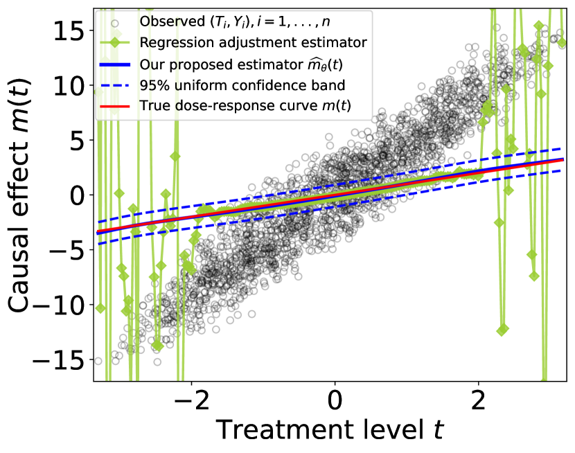
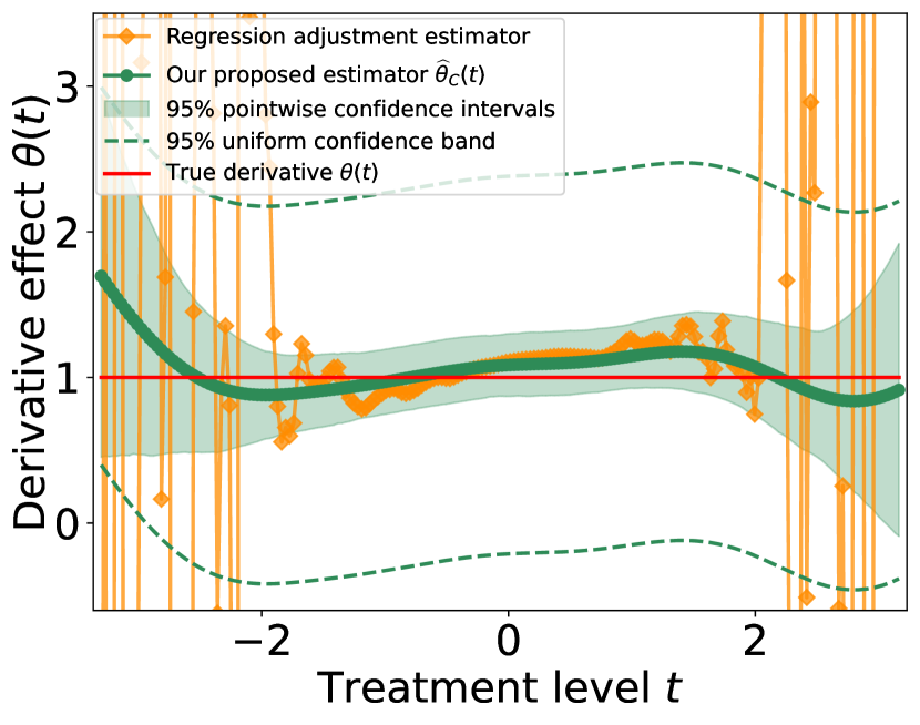
Figure 2: Simulation results under the linear confounding model (19). Left: The estimated dose-response curves by usual regression adjustment and our proposed estimators overlain with the true one $m(t)$. Right: The estimated derivatives of the dose-response curve by usual regression adjustment and our proposed estimators overlain with the true one $\theta(t)$. The middle and right panels also present the 95% confidence intervals and/or uniform confidence bands from our proposed estimators as shaded regions and dashed lines, respectively.

$\bullet$ Nonlinear Confounding Model: We consider the following nonlinear effect model with

$$\begin{split}&Y=T^{2}+T+10Z+\epsilon,\quad T=\cos\left(\pi Z^{3}\right)+\frac{Z}{4}+E,\quad Z=4S_{1}+S_{2},\\ &\quad\text{ and }\quad\bm{S}=(S_{1},S_{2})\sim\text{Uniform}[-1,1]^{2}\subset\mathbb{R}^{2},\end{split}$$ (20)

where $E\sim\text{Uniform}[-0.1,0.1]$ and $\epsilon\sim\mathcal{N}(0,1)$. Again, due to the nonlinear confounding effect $\cos(\pi Z)$ and small treatment variation $E$, the positivity condition (A0) fails on the generated data from (20). We also note that the debiased estimator of $m(t)$ proposed by Takatsu and Westling (2022) (and similarly, Kennedy et al. 2017) is incapable of recovering $m(t)$ under this data model, because some of their pseudo-outcomes have invalid values caused by nearly zero estimated conditional densities of $p(t|\bm{s})$.

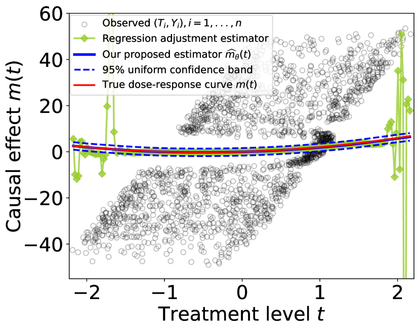
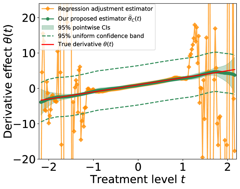
Figure 3: Simulation results under the nonlinear confounding model (20). See Fig 2 for the description of each panel.

Because of the presence of confounding variables, simply regressing $Y_{i}$’s to $T_{i}$’s in the generated data from each of the above models will give rise to biased estimates of $m(t)$. We apply both the proposed integral estimator $\widehat{m}_{\theta}(t)$ and localized derivative estimator $\widehat{\theta}_{C}(t)$ with bootstrap inferences in Section 3.3 to the generated data respectively. For comparisons, we also implement the usual regression adjustment estimators using the (partial) local quadratic regression (10) under the same choices of bandwidth parameters. The results are shown in Fig 1, Fig 2, and Fig 3. Note that the regression adjustment estimators are extremely unstable, especially around the boundary of the marginal support $\mathcal{T}$. Due to the failure of (A0), fine-tuning the bandwidth parameters $h,b$ will not ameliorate the stability and consistency of regression adjustment estimators. On the contrary, our proposed estimators can recover the true dose-response curves and its derivatives with relatively narrow pointwise confidence intervals and uniform bands.

5.3 Case Study: Effect of PM_2.5 on Cardiovascular Mortality Rate

Air pollution, especially fine particulate matter with diameters less than 2.5 $\unit{}$ (PM_2.5), is known to contribute to an increase in cardiovascular diseases (Brook et al., 2010; Krittanawong et al., 2023). Some recent studies also identify a positive association between the PM_2.5 level ($\unit{}/m^{3}$) and the county-level cardiovascular mortality rate (CMR; deaths/100,000 person-years) in the United States after controlling for socioeconomic factors (Wyatt et al., 2020a).

To showcase the applicability of our proposed integral and its derivative estimators, we apply them to analyzing the PM_2.5 and CMR data in Wyatt et al. (2020b). The data contain average annual CMR for outcome $Y$ and PM_2.5 concentration for treatment/exposure $T$ from 1990 to 2010 within $n=2132$ counties, which were obtained from the US National Center for Health Statistics and Community Multiscale Air Quality modeling system, respectively. Our covariate vector $\bm{S}\in\mathbb{R}^{10}$ comprises two parts of confounding variables. The first part consists of two spatial confounding variables, latitude and longitude of each county, that helps incorporate the spatial dependence. The second part includes eight county-level socioeconomic factors acquired from the US census: population in 2000, civilian unemployment rate, median household income, percentage of female households with no spouse, percentage of vacant housing units, percentage of owner occupied housing units, percentage of high school graduates or above, and percentage of households below poverty. For each county in a given year, we use the closest records from a US census year (1990, 2000, or 2010) as the values of its socioeconomic variables and then average the values of $Y,T,\bm{S}$ for each county over these 21 years as the final data. Finally, similar to Takatsu and Westling (2022), we focus on the values of PM_2.5 between 2.5 $\unit{}/m^{3}$ and 11.5 $\unit{}/m^{3}$ to avoid boundary effects.

We apply our proposed integral estimator (8) and localized derivative estimator (12) to the final data with the choices of bandwidth parameters in Section 5.1. To take the magnitude differences of treatment $T$ and covariates in $\bm{S}$ into consideration, we multiply the (coordinatewise) standard deviations of $T$ and $\bm{S}$ on the data to $h_{ROT},\bm{b}_{ROT}$ respectively and set $C_{h}=7,C_{b}=20$ to smooth out the estimated derivatives. To study the effects of confounding, we also consider regressing $Y$ on $T$ only via local quadratic regression estimators as well as fitting $Y$ on $T$ and spatial locations only via our proposed estimators. The results in the left panel of Fig 4 demonstrate that the effects of confounding. Before controlling any confounding variables, the fitted curve is not monotonic and peaks at around 8 $\unit{}/m^{3}$. After controlling for spatial locations, it becomes flatter but still decreases when PM_2.5 level is above 8 $\unit{}/m^{3}$. Only when we incorporate both spatial and socioeconomic covariates can the estimated relationship between PM_2.5 and CMR becomes monotonically increasing. The estimated changing rate of CMR with respect to PM_2.5 in the right panel of Fig 4 reveals the same conclusion from a different angle. More interestingly, after we adjust for all available confounding variables, the changing rate of CMR and its 95% confidence intervals flatten out and are unanimously above 0 when the PM_2.5 level is below 9 $\unit{}/m^{3}$. This indicates a strong signal of a positive association between the PM_2.5 level and CMR. However, when the PM_2.5 level is above 10 $\unit{}/m^{3}$, it is unclear whether PM_2.5 still positively contributes to cardiovascular mortality, possibly due to other competing risks (Leiser et al., 2019). Our findings generally align with the conclusions in Wyatt et al. (2020a); Takatsu and Westling (2022), but the superiority of our proposed estimators comes from two aspects. First, we estimate not only the relationship between PM_2.5 and CMR but also its derivative function, providing new insights into their association. Second, our proposed estimators are capable of resolving the potential violation of the positivity condition (A0) and thus lead to convincing conclusions in this observational study.

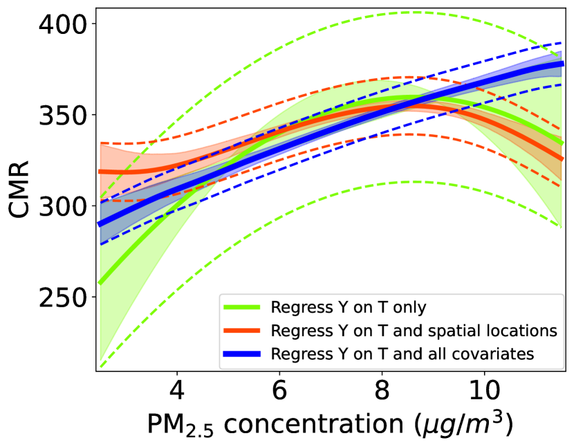
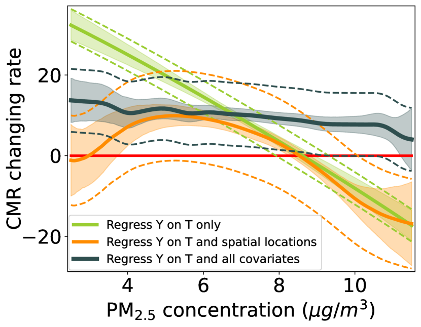
Figure 4: Estimated relationships between the PM_2.5 concentration and CMR or its changing rate at the county level. Left: The estimated CMR with respect to the PM_2.5 concentration. Right: The estimated changing rates of CMR with respect to the PM_2.5 concentration. We also present the 95% confidence intervals and uniform confidence bands as shaded regions and dashed lines respectively for each regression scenario.

6 Discussion

In summary, this paper studies nonparametric inference on the dose-response curve and its derivative function via innovative integral and localized derivative estimators. The main advantage of our proposed estimators is that they can consistently recover and infer the dose-response curve and its derivative without assuming the unrealistically strong positivity condition (A0) under the context of continuous treatments. We establish the consistency and bootstrap validity of the proposed estimators when nuisance functions are estimated by kernel smoothing methods but without requiring explicit undersmoothing on bandwidth parameters. Simulation studies and real-world applications demonstrate the effectiveness of our proposed estimators in addressing the failure of (A0). There are several future directions that can further advance the impacts of our proposed estimators.

1. Estimation of nuisance parameters/functions: The proposed integral estimator (8) and localized derivative estimator (12) require us to estimate two nuisance functions, the partial derivative $\frac{\partial}{\partial t}\mu(t,\bm{s})$ and the conditional CDF $P(\bm{s}|t)$. When we focus on the kernel smoothing methods, the finite-sample performances of our integral estimator (8) and localized derivative estimator (12) depend on the choices of three bandwidth parameters $h,b,\hslash>0$. We only consider the rule-of-thumb and normal reference bandwidth selection methods in this paper, but it would be of research interest to study how the bandwidth choices can be improved through the plug-in rule (Ruppert et al., 1995) or cross-validation (Li and Racine, 2004). More broadly, other estimators, such as regression splines for $\frac{\partial}{\partial t}\mu(t,\bm{s})$ (Friedman, 1991; Zhou and Wolfe, 2000) and nearest neighbor-type or local logistic approaches for $P(\bm{s}|t)$ (Stute, 1986; Hall et al., 1999), are also be applied to estimating the nuisance functions and may lead to better performances of our proposed estimators $\widehat{\theta}_{C}(t)$ and $\widehat{m}_{\theta}(t)$.

2. IPTW and doubly robust estimators: Our proposed estimators (8) and (12) are based on the idea of regression adjustment. Naturally, it would also be interesting to investigate how to leverage our integral and localized techniques to resolve the positivity requirement in the existing generalized propensity score-based approaches (Hirano and Imbens, 2004; Imai and van Dyk, 2004) and doubly robust methods (Kennedy et al., 2017; Westling et al., 2020; Colangelo and Lee, 2020; Semenova and Chernozhukov, 2021; Bonvini and Kennedy, 2022) for estimating the dose-response curve and its derivative function.

3. Additive model diagnostics: Assumption A2 is vital to the consistency of our proposed estimators, and it is unclear if this assumption holds beyond the additive confounding model (3). However, it is possible to utilize our estimators to test the correctness of the additive structure in (3). Under the positivity condition (A0), one can test (3) by estimating the absolute difference of $\left|\mathbb{E}\left[\frac{\partial}{\partial t}\mu(t,\bm{S})\right]-\mathbb{E}\left[\frac{\partial}{\partial t}\mu(t,\bm{S})\big{|}T=t\right]\right|$ from 0 via the regression adjustment estimator $\widehat{\theta}_{RA}(t)$ in Remark 1 and our estimator $\widehat{\theta}_{C}(t)$ in (12). Other testing procedures, such as the marginal integration regression method (Linton and Nielsen, 1995), are also applicable. When the positivity condition (A0) is violated, the partial derivative $\beta_{2}(t,\bm{s})=\frac{\partial}{\partial t}\mu(t,\bm{s})$ is still independent of $\bm{s}$ for any $t\in\mathcal{T}$ under (3), and our estimator $\widehat{\beta}_{2}(t,\bm{s})$ in (10) should not depend on $\bm{s}$ asymptotically. It suggests that statistical quantities, such as $\Theta(t)=\sup_{\bm{s}\in\mathcal{S}(t)}\left|\widehat{\beta}_{2}(t,\bm{s})-\widehat{\theta}_{C}(t)\right|$ and $\Theta=\int_{\mathcal{T}}\Theta(t)\,dt$, should converge to 0 as $n\to\infty$. Thus, one may derive the limiting distribution of $\Theta(t)$ or $\Theta$ to carry out a procedure for statistically testing the additive confounding model (3) without assuming (A0).

4. Violation of ignorability (Assumption A1(b)): In observational studies, there could be some unmeasured confounding variables that go beyond our covariate vector $\bm{S}\in\mathcal{S}\subset\mathbb{R}^{d}$ and bias our inference (VanderWeele, 2008). Hence, it is important to analyze the sensitivities of the dose-response curve and its derivative with respect to the violation of ignorability. In this scenario, the instrumental variable model (Kilbertus et al., 2020) and the Riesz-Frechet representation technique (Chernozhukov et al., 2022) might be useful for the analysis. As an alternative, one can also incorporate an additional high-dimensional covariate vector $\bm{Z}\in\mathbb{R}^{d^{\prime}}$ into our model (2) to avoid unmeasured confounding variables. However, since nonparametric estimations on $m(t)$ and $\theta(t)$ have slow rates of convergence when $d^{\prime}$ is large, one may consider imposing a linear form on $\bm{Z}$ so that

$$\mathbb{E}\left(Y|T=t,\bm{S}=\bm{s},\bm{Z}=\bm{z}\right)=m(t)+\eta(\bm{s})+\vartheta^{T}\bm{z}$$

or utilize some orthogonalization techniques in Section 4.3 of Rothenhäusler and Yu (2019) to conduct valid inference. We will leave them as future works.

Contents

[sections] [sections]l0

The supplementary material contains the proofs of main results in the paper and other auxiliary technical results.

Appendix A Nonparametric Bounds Under Zero Treatment Variations

In this section, we study nonparametric bounds on the dose-response curve $m(t)$ and its derivative function $\theta(t)$ under the additive confounding model (3) when the treatment variation $E$ has zero variance. We will leave the derivations of nonparametric bounds under the general model (2) as a future direction.

A.1 Nonparametric Bound on $m(t)$

Recall from Section 2.2 that when $\mathrm{Var}(E)=0$, the conditional mean outcome function $\mu(t,\bm{s})$ can only be identified on the lower dimensional surface $\left\{(t,\bm{s})\in\mathcal{T}\times\mathcal{S}:t=f(\bm{s})\right\}$ so that

$$\mu\left(f(\bm{s}),\bm{s}\right)=\bar{m}\left(f(\bm{s})\right)+\eta(\bm{s})=m\left(f(\bm{s})\right)+\eta(\bm{s}).$$ (21)

Given that $\mathrm{Var}(E)=0$, we can always fit the relation $T=f(\bm{S})$ from the observed data. Hence, we assume that the function $f$ is known for any $\bm{s}\in\mathcal{S}$ in the sequel. To obtain a nonparametric bound for all the possible values that $m(t)$ can take, we impose the following assumption on the magnitude of the random effect function $\eta:\mathcal{S}\to\mathbb{R}$ in (3); see Manski (1990) for related discussions.

Assumption A7 (Bounded random effect).

Let $L_{f}(t)=\left\{\bm{s}\in\mathcal{S}:f(\bm{s})=t\right\}$ be a level set of the function $f:\mathcal{S}\to\mathbb{R}$ at $t\in\mathcal{T}$. There exists a constant $\rho_{1}>0$ such that

$$\rho_{1}\geq\max\left\{\sup_{t\in\mathcal{T}}\sup_{\bm{s}\in L_{f}(t)}|\eta(\bm{s})|,\;\frac{\sup_{t\in\mathcal{T}}\sup_{\bm{s}\in L_{f}(t)}\mu(f(\bm{s}),\bm{s})-\inf_{t\in\mathcal{T}}\inf_{\bm{s}\in L_{f}(t)}\mu(f(\bm{s}),\bm{s})}{2}\right\}.$$

By (21) and the first lower on $\rho_{1}\geq\sup_{t\in\mathcal{T}}\sup_{\bm{s}\in L_{f}(t)}|\eta(\bm{s})|$ in Assumption A7, we know that

$$\left|\mu(f(\bm{s}),\bm{s})-m(t)\right|=|\eta(\bm{s})|\leq\rho_{1}$$

for any $\bm{s}\in L_{f}(t)$. It also implies that

$$\begin{split}m(t)&\in\bigcap_{\bm{s}\in L_{f}(t)}\left[\mu(f(\bm{s}),\bm{s})-\rho_{1},\,\mu(f(\bm{s}),\bm{s})+\rho_{1}\right]\\ &=\left[\sup_{\bm{s}\in L_{f}(t)}\mu(f(\bm{s}),\bm{s})-\rho_{1},\,\inf_{\bm{s}\in L_{f}(t)}\mu(f(\bm{s}),\bm{s})+\rho_{1}\right],\end{split}$$ (22)

which is the nonparametric bound on $m(t)$ that contains all the possible values of $m(t)$ for any fixed $t\in\mathcal{T}$ when $\mathrm{Var}(E)=0$. Notice that this bound (22) is well-defined and nonempty under the second lower bound on $\rho_{1}$ in Assumption A7.

A.2 Nonparametric Bound on $\theta(t)$

We already know that $\mu(f(\bm{s}),\bm{s})$ and $f(\bm{s})$ can be identified even when $\mathrm{Var}(E)=0$, so their derivatives with respect to $\bm{s}$ are also identifiable. Hence, we assume that the functions $\nabla_{\bm{s}}\mu(f(\bm{s}),\bm{s})$ and $\nabla f(\bm{s})$ are known for any $\bm{s}\in\mathcal{S}$ in the sequel. The nonparametric bound on the dose-response curve $m(t)$ involves an upper bound on the random effect function $\eta:\mathcal{S}\to\mathbb{R}$ (recall Assumption A7), while the nonparametric bound on the derivative function $\theta(t)$ requires some constraints on the gradient $\nabla\eta(\bm{s})$ of the random effect function as follows.

Assumption A8 (Constraints on the random effect gradient).

Let $L_{f}(t)=\left\{\bm{s}\in\mathcal{S}:f(\bm{s})=t\right\}$ be a level set of the function $f:\mathcal{S}\to\mathbb{R}$ at $t\in\mathcal{T}$. There exist constants $\rho_{2},\rho_{3}>0$ such that

$$\rho_{3}\leq\inf_{t\in\mathcal{T}}\inf_{\bm{s}\in L_{f}(t)}\left|\left|\nabla\eta(\bm{s})\right|\right|_{\min}\leq\sup_{t\in\mathcal{T}}\sup_{\bm{s}\in L_{f}(t)}\left|\left|\nabla\eta(\bm{s})\right|\right|_{\max}\leq\rho_{2}$$

and

$$\sup_{t\in\mathcal{T}}\sup_{\bm{s}\in L_{f}(t)}\max_{j=1,...,d}\left[\frac{v_{j}(\bm{s})-\mathrm{sign}(g_{j}(\bm{s}))\cdot\rho_{2}}{g_{j}(\bm{s})}\right]\leq\inf_{t\in\mathcal{T}}\inf_{\bm{s}\in L_{f}(t)}\min_{j=1,...,d}\left[\frac{v_{j}(\bm{s})+\mathrm{sign}(g_{j}(\bm{s}))\cdot\rho_{2}}{g_{j}(\bm{s})}\right],$$

where $\left|\left|\nabla\eta(\bm{s})\right|\right|_{\min}=\min_{j=1,...,d}\left|\frac{\partial}{\partial s_{j}}\eta(\bm{s})\right|$, $\left|\left|\nabla\eta(\bm{s})\right|\right|_{\max}=\max_{j=1,...,d}\left|\frac{\partial}{\partial s_{j}}\eta(\bm{s})\right|$, $v_{j}(\bm{s})=\frac{\partial}{\partial s_{j}}\mu(f(\bm{s}),\bm{s})$, and $g_{j}(\bm{s})=\frac{\partial}{\partial s_{j}}f(\bm{s})$ for $j=1,...,d$.

The first inequality in Assumption A8 ensures that we can derive a finite and meaningful nonparametric bound on $\theta(t)$ for any $t\in\mathcal{T}$. In particular, a direct calculation shows that

$$\nabla_{\bm{s}}\mu(f(\bm{s}),\bm{s}) =\nabla_{\bm{s}}m(f(\bm{s}))+\nabla\eta(\bm{s})$$

$$=m^{\prime}(f(\bm{s}))\cdot\nabla f(\bm{s})+\nabla\eta(\bm{s})$$

$$=\theta(t)\cdot\nabla f(\bm{s})+\nabla\eta(\bm{s})$$

for all $\bm{s}\in L_{f}(t)$. This indicates that

$$\left|\frac{\partial}{\partial s_{j}}\mu(f(\bm{s}),\bm{s})-\theta(t)\cdot\frac{\partial}{\partial s_{j}}f(\bm{s})\right|=\left|v_{j}(\bm{s})-\theta(t)\cdot g_{j}(\bm{s})\right|=\left|\frac{\partial}{\partial s_{j}}\eta(\bm{s})\right|\leq\rho_{2}$$

for $j=1,...,d$ and therefore, a nonparametric bound on $\theta(t)$ is given by

$$\theta(t)\in\bigcap_{j=1}^{d}\left[\frac{v_{j}(\bm{s})-\mathrm{sign}(g_{j}(\bm{s}))\cdot\rho_{2}}{g_{j}(\bm{s})},\;\frac{v_{j}(\bm{s})+\mathrm{sign}(g_{j}(\bm{s}))\cdot\rho_{2}}{g_{j}(\bm{s})}\right].$$ (23)

This bound is well-defined and nonempty under the second inequality in Assumption A8. More importantly, the nonparametric bound (23) sheds light on the critical role of the covariate effect function $f$ of $\bm{S}$ on treatment $T$ in bounding the possible value of $\theta(t)$. Specifically, when the variation of $f$ is higher (i.e., $\nabla f(\bm{s})$ is larger in its magnitude), the nonparametric bound (23) will be tighter.

Appendix B Proofs

This section consists of the proofs for theorems, lemmas, and propositions in the main paper as well as other auxiliary results.

B.1 Proof of Proposition 1

Proposition 1 (Properties of the additive confounding model (3)).

Let $\theta_{M}(t)=\mathbb{E}\left[\frac{\partial}{\partial t}\mu(t,\bm{S})\right]$ and $\theta_{C}(t)=\mathbb{E}\left[\frac{\partial}{\partial t}\mu(t,\bm{S})\big{|}T=t\right]$, where $\mu(t,\bm{s})=\mathbb{E}\left[Y|T=t,\bm{S}=\bm{s}\right]$. Under the additive confounding model (3) with $\mbox{$\mathbb{E}$}\left[\eta(\bm{S})\right]=0$, the following results hold for all $t\in\mathcal{T}$:

1. $m(t)=\bar{m}(t)$.

2. $m(t)\neq\mbox{$\mathbb{E}$}(Y|T=t)=\bar{m}(t)+\mbox{$\mathbb{E}$}\left[\eta(\bm{S})|T=t\right]$ when $\mbox{$\mathbb{E}$}\left[\eta(\bm{S})|T=t\right]\neq 0$.

3. $\theta(t)=\theta_{M}(t)=\theta_{C}(t)$.

4. $\theta(t)\neq\frac{d}{dt}\mbox{$\mathbb{E}$}\left[\mu(t,\bm{S})|T=t\right]=\theta(t)+\frac{d}{dt}\mbox{$\mathbb{E}$}\left[\eta(\bm{S})|T=t\right]$ when $\frac{d}{dt}\mbox{$\mathbb{E}$}\left[\eta(\bm{S})|T=t\right]\neq 0$.

5. $\mathbb{E}\left[\mu(T,\bm{S})\right]=\mathbb{E}\left[m(T)\right]$ even when $\mbox{$\mathbb{E}$}\left[\eta(\bm{S})\right]\neq 0$.

The above results hold even if the treatment variation $E=0$ almost surely.

Proof of Proposition 1.

All the results follow from some simple calculations and the fact that

$$\mu(t,\bm{s})=\mbox{$\mathbb{E}$}\left(Y|T=t,\bm{S}=\bm{s}\right)=\bar{m}(t)+\eta(\bm{s})$$

under the additive confounding model (3).

(a) Given that $\mbox{$\mathbb{E}$}\left[\eta(\bm{S})\right]=0$, we note that

$$m(t) =\mbox{$\mathbb{E}$}\left[\mu(t,\bm{S})\right]=\mbox{$\mathbb{E}$}\left[\mbox{$\mathbb{E}$}\left(Y|T=t,\bm{S}\right)\right]=\mbox{$\mathbb{E}$}\left[\bar{m}(t)+\eta(\bm{S})\right]=\bar{m}(t).$$

(b) By (a), we know that

$$\mbox{$\mathbb{E}$}\left(Y|T=t\right)=\bar{m}(t)+\mbox{$\mathbb{E}$}\left[\eta(\bm{S})|T=t\right]\neq\bar{m}(t)=m(t)$$

when $\mbox{$\mathbb{E}$}\left[\eta(\bm{S})|T=t\right]\neq 0$.

(c) First, we notice that

$$\theta_{M}(t)\equiv\mbox{$\mathbb{E}$}\left[\frac{\partial}{\partial t}\mu(t,\bm{S})\right]=\mbox{$\mathbb{E}$}\left[\bar{m}^{\prime}(t)\right]=\bar{m}^{\prime}(t)=m^{\prime}(t)=\theta(t).$$

In addition, we also have that

$$\theta_{C}(t) \equiv\mbox{$\mathbb{E}$}\left[\frac{\partial}{\partial t}\mu(t,\bm{S})\Big{|}T=t\right]=\mbox{$\mathbb{E}$}\left[\bar{m}^{\prime}(t)|T=t\right]=\bar{m}^{\prime}(t)=\theta(t).$$

(d) From (c), we know that

$$\frac{d}{dt}\mbox{$\mathbb{E}$}\left[\mu(t,\bm{S})|T=t\right]=\frac{d}{dt}\left[\bar{m}(t)+\mbox{$\mathbb{E}$}\left(\eta(\bm{S})|T=t\right)\right]=\bar{m}^{\prime}(t)+\frac{d}{dt}\mbox{$\mathbb{E}$}\left(\eta(\bm{S})|T=t\right)\neq\theta(t)$$

when $\frac{d}{dt}\mbox{$\mathbb{E}$}\left[\eta(\bm{S})|T=t\right]\neq 0$.

(e) We know that the left hand side is equal to

$$\mathbb{E}\left[\mu(T,\bm{S})\right]=\mathbb{E}\left[\bar{m}(T)+\eta(\bm{S})\right]=\mathbb{E}\left[\bar{m}(T)\right]+\mathbb{E}\left[\eta(\bm{S})\right],$$

while the right hand side is given by

$$\mathbb{E}\left[m(T)\right]=\mathbb{E}\left\{\bar{m}(T)+\mathbb{E}\left[\eta(\bm{S})\right]\right\}=\mathbb{E}\left[\bar{m}(T)\right]+\mathbb{E}\left[\eta(\bm{S})\right].$$

This result thus holds even when $\mathbb{E}\left[\eta(\bm{S})\right]\neq 0$.

Finally, when deriving (a)-(e), we do not impose any condition on the treatment variation $E$, the results hold no matter what distribution of $E$ is. ∎

B.2 Proof of Lemma 2

Before proving Lemma 2, we give a complete statement of the asymptotic expressions for the conditional variance and bias of $\widehat{\beta}_{2}(t,\bm{s})$ as follows.

Lemma 2 (Pointwise convergence of $\widehat{\beta}_{2}(t,\bm{s})$).

Suppose that Assumptions A3, A4, A5, and A6(a) hold under the confounding model (2). Let $\widehat{\beta}_{2}(t,\bm{s})$ be the second element of $\widehat{\bm{\beta}}(t,\bm{s})\in\mathbb{R}^{q+1}$, $\beta_{2}(t,\bm{s})=\frac{\partial}{\partial t}\mu(t,\bm{s})$, and $\mathbb{X}=\left\{(T_{i},\bm{S}_{i})\right\}_{i=1}^{n}$. Then, for any $(t,\bm{s})\in\mathcal{E}^{\circ}$ and $q>0$, as $h,b,\frac{b^{4}}{h}\to 0$ and $nh^{3}b^{d}\to\infty$, we know that the asymptotic conditional covariance of $\widehat{\beta}_{2}(t,\bm{s})\in\mathbb{R}$ is given by

$$\mathrm{Var}\left[\widehat{\beta}_{2}(t,\bm{s})\big{|}\mathbb{X}\right] =\frac{\sigma^{2}}{nh^{3}b^{d}\cdot p(t,\bm{s})}\left[\bm{e}_{2}^{T}\bm{M}_{q}^{-1}\bm{M}_{q}^{*}\bm{M}_{q}^{-1}\bm{e}_{2}+O\left(\max\{h,b\}\right)+O_{P}\left(\sqrt{\frac{1}{nhb^{d}}}\right)\right],$$

and the asymptotic conditional bias is given by

$$\mathrm{Bias}\left[\widehat{\beta}_{2}(t,\bm{s})\big{|}\mathbb{X}\right]=\begin{cases}\frac{1}{p(t,\bm{s})}\left[h^{q+1}\tau_{q}^{\text{odd}}+b^{2}\tau_{q}^{*}+O\left(\frac{b^{4}}{h}\right)+o_{P}\left(\sqrt{\frac{1}{nhb^{d}}}\right)\right]&q\text{ is odd},\\ \frac{1}{p(t,\bm{s})}\left[h^{q}\tau_{q}^{\text{even}}+b^{2}\tau_{q}^{*}+O\left(\frac{b^{4}}{h}\right)+o_{P}\left(\sqrt{\frac{1}{nhb^{d}}}\right)\right]&q\text{ is even}.\end{cases}$$

Here, $\mathcal{E}^{\circ}$ is the interior of the support $\mathcal{E}\subset\mathcal{T}\times\mathcal{S}$, $\bm{e}_{2}=(0,1,0,...,0)^{T}\in\mathbb{R}^{q+1}$, $\bm{M}_{q}=\left(\kappa_{i+j-2}^{(T)}\right)_{1\leq i,j\leq q+1}\in\mathbb{R}^{(q+1)\times(q+1)}$, $\bm{M}_{q}^{*}=\left(\nu_{i+j-2}^{(T)}\nu_{0}^{(S)}\right)_{1\leq i,j\leq q+1}\in\mathbb{R}^{(q+1)\times(q+1)}$, $\tau_{q}^{\text{odd}}=\frac{\bm{e}_{2}^{T}\bm{M}_{q}^{-1}\bm{\tau}_{q}}{h}$ when $q$ is odd and $\tau_{q}^{\text{even}}=\bm{e}_{2}^{T}\bm{M}_{q}^{-1}\bm{\tau}_{q}$ when $q$ is even, as well as $\tau_{q}^{*}=\frac{\bm{e}_{2}^{T}\bm{M}_{q}^{-1}\bm{\tau}_{q}^{*}}{b}$, where

$$\bm{\tau}_{q}=\left[\frac{\partial^{q+1}}{\partial t^{q+1}}\mu(t,\bm{s})\right]\frac{1}{(q+1)!}\begin{bmatrix}\begin{pmatrix}\kappa_{q+j}^{(T)}\cdot p(t,\bm{s})+h\cdot\kappa_{q+j+1}^{(T)}\cdot\frac{\partial}{\partial t}p(t,\bm{s})\end{pmatrix}_{1\leq j\leq q+1}\\ \begin{pmatrix}b\kappa_{q+1}^{(T)}\kappa_{2,j-q-1}^{(S)}\cdot\frac{\partial}{\partial s_{j-q-1}}p(t,\bm{s})\end{pmatrix}_{q+1<j\leq q+1+d}\end{bmatrix}\in\mathbb{R}^{(q+1+d)\times(q+1+d)},$$

$$\bm{\tau}_{q}^{*}=\begin{bmatrix}\begin{pmatrix}b\sum_{\ell=1}^{d}\left[\frac{\partial^{2}}{\partial t\partial s_{\ell}}\mu(t,\bm{s})\right]\kappa_{j}^{(T)}\kappa_{2,\ell}^{(S)}\cdot\frac{\partial}{\partial s_{\ell}}p(t,\bm{s})\end{pmatrix}_{1\leq j\leq q+1}\\ \begin{pmatrix}h\left[\frac{\partial^{2}}{\partial t\partial s_{j-q-1}}\mu(t,\bm{s})\right]\kappa_{2}^{(T)}\kappa_{2,j-q-1}^{(S)}\cdot\frac{\partial}{\partial t}p(t,\bm{s})\end{pmatrix}_{q+1<j\leq q+1+d}\end{bmatrix}\in\mathbb{R}^{(q+1+d)\times(q+1+d)},$$

and

$$\widetilde{\bm{\tau}}_{q}=\begin{bmatrix}\begin{pmatrix}\kappa_{j-1}^{(T)}p(t,\bm{s})\sum_{\ell=1}^{d}\frac{\kappa_{2,\ell}^{(S)}}{2}\left(\frac{\partial^{2}}{\partial s_{\ell}^{2}}\mu(t,\bm{s})\right)\end{pmatrix}_{1\leq j\leq q+1}\\ \begin{pmatrix}b\sum_{\ell=1}^{d}\frac{\kappa_{2,j-q-1,\ell}^{(S)}}{2}\left[\frac{\partial^{2}}{\partial s_{\ell}^{2}}\mu(t,\bm{s})\right]\cdot\frac{\partial}{\partial s_{j-q-1}}p(t,\bm{s})\end{pmatrix}_{q+1<j\leq q+1+d}\end{bmatrix}\in\mathbb{R}^{(q+1+d)\times(q+1+d)}.$$

Furthermore, as $h,b,\frac{\max\{h,b\}^{4}}{h}\to 0$, and $nh^{3}b^{d}\to\infty$, we have that

$$\widehat{\beta}_{2}(t,\bm{s})-\beta_{2}(t,\bm{s})$$

$$=\begin{cases}O\left(h^{q+1}+b^{2}+\frac{b^{4}}{h}\right)+O_{P}\left(\sqrt{\frac{1}{nh^{3}b^{d}}}\right)&\text{ if }q\text{ is odd and }(t,\bm{s})\in\mathcal{E}^{\circ},\\ O\left(h^{q}+b^{2}+\frac{b^{4}}{h}\right)+O_{P}\left(\sqrt{\frac{1}{nh^{3}b^{d}}}\right)&\text{ if }q\text{ is even and }(t,\bm{s})\in\mathcal{E}^{\circ},\\ O\left(h^{q}+\frac{\max\{h,b\}^{4}}{h}\right)+O_{P}\left(\sqrt{\frac{1}{nh^{3}b^{d}}}\right)&\text{ if }q\text{ is an integer and }(t,\bm{s})\in\partial\mathcal{E}.\end{cases}$$

Proof of Lemma 2.

Recall from (10) that

$$\left(\widehat{\bm{\beta}}(t,\bm{s}),\widehat{\bm{\alpha}}(t,\bm{s})\right)^{T} =\left[\bm{X}^{T}(t,\bm{s})\bm{W}(t,\bm{s})\bm{X}(t,\bm{s})\right]^{-1}\bm{X}(t,\bm{s})^{T}\bm{W}(t,\bm{s})\bm{Y}$$

$$\equiv\left(\bm{X}^{T}\bm{W}\bm{X}\right)^{-1}\bm{X}^{T}\bm{W}\bm{Y}.$$

The proof of Lemma 2 has two major components, where we consider the cases when $(t,\bm{s})$ is an interior point or a boundary point of the support $\mathcal{E}$. When $(t,\bm{s})$ is an interior point of $\mathcal{E}$, we also divide the arguments into three steps that deal with the rates of convergence for the term $\bm{X}^{T}\bm{W}\bm{X}$, the conditional covariance term $\mathrm{Cov}\left[\left(\widehat{\bm{\beta}}(t,\bm{s}),\widehat{\bm{\alpha}}(t,\bm{s})\right)^{T}\right]$, and the conditional bias term $\mathrm{Bias}\left[\left(\widehat{\bm{\beta}}(t,\bm{s}),\widehat{\bm{\alpha}}(t,\bm{s})\right)^{T}\Big{|}\mathbb{X}\right]$ separately.
 

We first consider the case when $(t,\bm{s})$ is an interior point of the support $\mathcal{E}$, i.e., for any $(t_{1},\bm{s}_{1})\in\mathcal{T}\times\mathcal{S}$, $\frac{t_{1}-t}{h}$ and $\frac{\bm{s}_{1}-\bm{s}}{b}$ lie in the supports of $K_{T}$ and $K_{S}$ respectively when $h,b$ are small. Notice that under the confounding model (2), we have that

$$\mathrm{Cov}\left[\left(\widehat{\bm{\beta}}(t,\bm{s}),\widehat{\bm{\alpha}}(t,\bm{s})\right)^{T}\Big{|}\mathbb{X}\right] =\left(\bm{X}^{T}\bm{W}\bm{X}\right)^{-1}\bm{X}^{T}\bm{\Sigma}\bm{X}\left(\bm{X}^{T}\bm{W}\bm{X}\right)^{-1}$$

and

$$\mathrm{Bias}\left[\left(\widehat{\bm{\beta}}(t,\bm{s}),\widehat{\bm{\alpha}}(t,\bm{s})\right)^{T}\Big{|}\mathbb{X}\right] =\mathbb{E}\left[\left(\widehat{\bm{\beta}}(t,\bm{s}),\widehat{\bm{\alpha}}(t,\bm{s})\right)^{T}\right]-\left(\bm{\beta}(t,\bm{s}),\bm{\alpha}(t,\bm{s})\right)^{T}$$

$$=\left(\bm{X}^{T}\bm{W}\bm{X}\right)^{-1}\bm{X}^{T}\bm{W}\left[\begin{pmatrix}\mu(T_{1},\bm{S}_{1})\\ \vdots\\ \mu(T_{n},\bm{S}_{n})\end{pmatrix}-\bm{X}\begin{pmatrix}\bm{\beta}(t,\bm{s})\\ \bm{\alpha}(t,\bm{s})\end{pmatrix}\right],$$

where $\bm{\Sigma}\in\mathbb{R}^{n\times n}$ is a diagonal matrix as $\mathtt{Diag}\Big{(}\sigma^{2}K_{T}^{2}\left(\frac{T_{1}-t}{h}\right)K_{S}^{2}\left(\frac{\bm{S}_{1}-\bm{s}}{b}\right),...,\sigma^{2}K_{T}^{2}\left(\frac{T_{n}-t}{h}\right)K_{S}^{2}\left(\frac{\bm{S}_{n}-\bm{s}}{b}\right)\Big{)}$ and by Assumption A3 and Taylor’s expansion,

$$\left(\bm{\beta}(t,\bm{s}),\bm{\alpha}(t,\bm{s})\right)^{T}\equiv\left(\mu(t,\bm{s}),\frac{\partial}{\partial t}\mu(t,\bm{s}),...,\frac{1}{q!}\cdot\frac{\partial^{q}}{\partial t^{q}}\mu(t,\bm{s}),\frac{\partial}{\partial s_{1}}\mu(t,\bm{s}),...,\frac{\partial}{\partial s_{d}}\mu(t,\bm{s})\right)^{T}.$$

Step 1: Common term $\bm{X}^{T}\bm{W}\bm{X}$. Before deriving the asymptotic behaviors of the above conditional covariance matrix and bias, we first study the rates of convergence of $\bm{X}^{T}\bm{W}\bm{X}\in\mathbb{R}^{(q+1+d)\times(q+1+d)}$.

By direct calculations, we know that

$$\begin{split}&\left(\bm{X}^{T}\bm{W}\bm{X}\right)_{i,j}\\ &=\begin{cases}\sum\limits_{k=1}^{n}(T_{k}-t)^{i+j-2}K_{T}\left(\frac{T_{k}-t}{h}\right)K_{S}\left(\frac{\bm{S}_{k}-\bm{s}}{b}\right),\quad\quad 1\leq i,j\leq q+1,\\ \sum\limits_{k=1}^{n}(T_{k}-t)^{i-1}\left(S_{k,j-q-1}-s_{j-q-1}\right)K_{T}\left(\frac{T_{k}-t}{h}\right)K_{S}\left(\frac{\bm{S}_{k}-\bm{s}}{b}\right),\quad 1\leq i\leq q+1\text{ and }q+1<j\leq q+1+d,\\ \sum\limits_{k=1}^{n}\left(S_{k,i-q-1}-s_{i-q-1}\right)(T_{k}-t)^{j-1}K_{T}\left(\frac{T_{k}-t}{h}\right)K_{S}\left(\frac{\bm{S}_{k}-\bm{s}}{b}\right),\quad q+1<i\leq q+1+d\text{ and }1\leq j\leq q+1,\\ \sum\limits_{k=1}^{n}\left(S_{k,i-q-1}-s_{i-q-1}\right)\left(S_{k,j-q-1}-s_{j-q-1}\right)K_{T}\left(\frac{T_{k}-t}{h}\right)K_{S}\left(\frac{\bm{S}_{k}-\bm{s}}{b}\right),\quad q+1<i,j\leq q+1+d.\end{cases}\end{split}$$ (24)

Here, each sample $\bm{S}_{k}\in\mathcal{S}\subset\mathbb{R}^{d}$ is written as $\bm{S}_{k}=\left(S_{k,1},...,S_{k,d}\right)^{T}\in\mathbb{R}^{d}$. We now derive the asymptotic rates of convergence of the expectation and variance for each term in (24) under Assumptions A3, A4, and A6.

$\bullet$ Case I: $1\leq i,j\leq q+1$. We compute that

$$\mathbb{E}\left[\left(\bm{X}^{T}\bm{W}\bm{X}\right)_{i,j}\right]$$

$$=n\int_{\mathbb{R}\times\mathbb{R}^{d}}\left(\widetilde{t}-t\right)^{i+j-2}K_{T}\left(\frac{\widetilde{t}-t}{h}\right)K_{S}\left(\frac{\widetilde{\bm{s}}-\bm{s}}{b}\right)p(\widetilde{t},\widetilde{\bm{s}})\,d\widetilde{t}d\widetilde{\bm{s}}$$

$$\stackrel{{\scriptstyle\text{(i)}}}{{=}}nh^{i+j-1}b^{d}\int_{\mathbb{R}\times\mathbb{R}^{d}}u^{i+j-2}K_{T}(u)K_{S}(\bm{v})\cdot p(t+uh,\bm{s}+b\bm{v})\,dud\bm{v}$$

$$\stackrel{{\scriptstyle\text{(ii)}}}{{=}}nh^{i+j-1}b^{d}\int_{\mathbb{R}\times\mathbb{R}^{d}}u^{i+j-2}K_{T}(u)K_{S}(\bm{v})\left[p(t,\bm{s})+uh\cdot\frac{\partial}{\partial t}p(t,\bm{s})+b\bm{v}^{T}\frac{\partial}{\partial\bm{s}}p(t,\bm{s})+O\left(\max\{h,b\}^{2}\right)\right]dud\bm{v}$$

$$\stackrel{{\scriptstyle\text{(iii)}}}{{=}}nh^{i+j-1}b^{d}\left[\kappa_{i+j-2}^{(T)}\cdot p(t,\bm{s})+h\cdot\kappa_{i+j-1}^{(T)}\cdot\frac{\partial}{\partial t}p(t,\bm{s})+O\left(\max\{h,b\}^{2}\right)\right],$$

where (i) utilizes the changes of variables $u=\frac{\widetilde{t}-t}{h}$ and $\bm{v}=\frac{\widetilde{\bm{s}}-\bm{s}}{b}$, (ii) leverages the differentiability of $p(t,\bm{s})$ and apply Taylor’s expansion, as well as (iii) uses the symmetric properties of $K_{T},K_{S}$ with notations in Assumption A6(a). In addition, we calculate that

$$\mathrm{Var}\left[\left(\bm{X}^{T}\bm{W}\bm{X}\right)_{i,j}\right]$$

$$=n\cdot\mathrm{Var}\left[(T_{1}-t)^{i+j-2}K_{T}\left(\frac{T_{1}-t}{h}\right)K_{S}\left(\frac{\bm{S}_{1}-\bm{s}}{b}\right)\right]$$

$$\leq n\int_{\mathbb{R}\times\mathbb{R}^{d}}(\widetilde{t}-t)^{2i+2j-4}K_{T}^{2}\left(\frac{\widetilde{t}-t}{h}\right)K_{S}^{2}\left(\frac{\widetilde{\bm{s}}-\bm{s}}{b}\right)p(\widetilde{t},\widetilde{\bm{s}})\,d\widetilde{t}d\widetilde{\bm{s}}$$

$$=nh^{2i+2j-3}b^{d}\int_{\mathbb{R}\times\mathbb{R}^{d}}u^{2i+2j-4}K_{T}^{2}(u)K_{S}^{2}(v)p(t+uh,\bm{s}+b\bm{v})\,dud\bm{v}$$

$$=nh^{2i+2j-3}b^{d}\int_{\mathbb{R}\times\mathbb{R}^{d}}u^{2i+2j-4}K_{T}^{2}(u)K_{S}^{2}(v)\left[p(t,\bm{s})+uh\cdot\frac{\partial}{\partial t}p(t,\bm{s})+b\bm{v}^{T}\frac{\partial}{\partial\bm{s}}p(t,\bm{s})+O\left(\max\{h,b\}^{2}\right)\right]dud\bm{v}$$

$$=nh^{2i+2j-3}b^{d}\left[\nu_{2i+2j-4}^{(T)}\nu_{0}^{(S)}\cdot p(t,\bm{s})+h\cdot\nu_{2i+2j-3}^{(T)}\nu_{0}^{(S)}\cdot\frac{\partial}{\partial t}p(t,\bm{s})+O\left(\max\{h,b\}^{2}\right)\right].$$

The above calculations on $\mathbb{E}\left[\left(\bm{X}^{T}\bm{W}\bm{X}\right)_{i,j}\right]$ and $\mathrm{Var}\left[\left(\bm{X}^{T}\bm{W}\bm{X}\right)_{i,j}\right]$ imply that

$$\left(\bm{X}^{T}\bm{W}\bm{X}\right)_{i,j}$$

$$=\mathbb{E}\left[\left(\bm{X}^{T}\bm{W}\bm{X}\right)_{i,j}\right]+O_{P}\left(\sqrt{\mathrm{Var}\left[\left(\bm{X}^{T}\bm{W}\bm{X}\right)_{i,j}\right]}\right)$$

$$=nh^{i+j-1}b^{d}\left[\kappa_{i+j-2}^{(T)}\cdot p(t,\bm{s})+h\cdot\kappa_{i+j-1}^{(T)}\cdot\frac{\partial}{\partial t}p(t,\bm{s})+O\left(\max\{h,b\}^{2}\right)+O_{P}\left(\sqrt{\frac{1}{nhb^{d}}}\right)\right]$$

for any $1\leq i,j\leq q+1$.

$\bullet$ Case II: $1\leq i\leq q+1$ and $q+1<j\leq q+1+d$. We compute that

$$\mathbb{E}\left[\left(\bm{X}^{T}\bm{W}\bm{X}\right)_{i,j}\right]$$

$$=n\int_{\mathbb{R}\times\mathbb{R}^{d}}\left(\widetilde{t}-t\right)^{i-1}(\widetilde{s}_{j-q-1}-s_{j-q-1})K_{T}\left(\frac{\widetilde{t}-t}{h}\right)K_{S}\left(\frac{\widetilde{\bm{s}}-\bm{s}}{b}\right)p(\widetilde{t},\widetilde{\bm{s}})\,d\widetilde{t}d\widetilde{\bm{s}}$$

$$=nh^{i}b^{d+1}\int_{\mathbb{R}\times\mathbb{R}^{d}}u^{i-1}v_{j-q-1}K_{T}(u)K_{S}(\bm{v})p(t+hu,\bm{s}+b\bm{v})\,dud\bm{v}$$

$$=nh^{i}b^{d+1}\int_{\mathbb{R}\times\mathbb{R}^{d}}u^{i-1}v_{j-q-1}K_{T}(u)K_{S}(\bm{v})\left[p(t,\bm{s})+uh\cdot\frac{\partial}{\partial t}p(t,\bm{s})+b\bm{v}^{T}\frac{\partial}{\partial\bm{s}}p(t,\bm{s})+O\left(\max\{h,b\}^{2}\right)\right]dud\bm{v}$$

$$=nh^{i}b^{d+1}\left[b\cdot\kappa_{i-1}^{(T)}\kappa_{2,j-q-1}^{(S)}\cdot\frac{\partial}{\partial s_{j-q-1}}p(t,\bm{s})+O\left(\max\{h,b\}^{2}\right)\right]$$

and

$$\mathrm{Var}\left[\left(\bm{X}^{T}\bm{W}\bm{X}\right)_{i,j}\right]$$

$$=n\cdot\mathrm{Var}\left[(T_{1}-t)^{i-1}(S_{1,j-q-1}-s_{j-q-1})K_{T}\left(\frac{T_{1}-t}{h}\right)K_{S}\left(\frac{\bm{S}_{1}-\bm{s}}{b}\right)\right]$$

$$\leq n\int_{\mathbb{R}\times\mathbb{R}^{d}}(\widetilde{t}-t)^{2i-2}(\widetilde{s}_{j-q-1}-s_{j-q-1})^{2}K_{T}^{2}\left(\frac{\widetilde{t}-t}{h}\right)K_{S}^{2}\left(\frac{\widetilde{\bm{s}}-\bm{s}}{b}\right)p(\widetilde{t},\widetilde{\bm{s}})\,d\widetilde{t}d\widetilde{\bm{s}}$$

$$=nh^{2i-1}b^{d+2}\int_{\mathbb{R}\times\mathbb{R}^{d}}u^{2i-2}v_{j-q-1}^{2}K_{T}^{2}(u)K_{S}^{2}(\bm{v})\left[p(t,\bm{s})+uh\cdot\frac{\partial}{\partial t}p(t,\bm{s})+b\bm{v}^{T}\frac{\partial}{\partial\bm{s}}p(t,\bm{s})+O\left(\max\{h,b\}^{2}\right)\right]dud\bm{v}$$

$$=nh^{2i-1}b^{d+2}\left[\nu_{2i-2}^{(T)}\nu_{2,j-q-1}^{(S)}\cdot p(t,\bm{s})+O(h)+O\left(\max\{h,b\}^{2}\right)\right].$$

These two terms indicate that

$$\left(\bm{X}^{T}\bm{W}\bm{X}\right)_{i,j} =\mathbb{E}\left[\left(\bm{X}^{T}\bm{W}\bm{X}\right)_{i,j}\right]+O_{P}\left(\sqrt{\mathrm{Var}\left[\left(\bm{X}^{T}\bm{W}\bm{X}\right)_{i,j}\right]}\right)$$

$$=nh^{i}b^{d+1}\left[b\cdot\kappa_{i-1}^{(T)}\kappa_{2,j-q-1}^{(S)}\cdot\frac{\partial}{\partial s_{j-q-1}}p(t,\bm{s})+O\left(\max\{h,b\}^{2}\right)+O_{P}\left(\sqrt{\frac{1}{nhb^{d}}}\right)\right]$$

for any $1\leq i\leq q+1$ and $q+1<j\leq q+1+d$.

$\bullet$ Case III: $q+1<i\leq q+1+d$ and $1\leq j\leq q+1$. By swapping the roles of $i$ and $j$ in our calculations for Case 2, we obtain that

$$\left(\bm{X}^{T}\bm{W}\bm{X}\right)_{i,j} =nh^{j}b^{d+1}\left[b\cdot\kappa_{j-1}^{(T)}\kappa_{2,i-q-1}^{(S)}\cdot\frac{\partial}{\partial s_{i-q-1}}p(t,\bm{s})+O\left(\max\{h,b\}^{2}\right)+O_{P}\left(\sqrt{\frac{1}{nhb^{d}}}\right)\right]$$

for any $q+1<i\leq q+1+d$ and $1\leq j\leq q+1$.

$\bullet$ Case IV: $q+1<i,j\leq q+1+d$. We compute that

$$\mathbb{E}\left[\left(\bm{X}^{T}\bm{W}\bm{X}\right)_{i,j}\right]$$

$$=n\int_{\mathbb{R}\times\mathbb{R}^{d}}(\widetilde{s}_{i-q-1}-s_{i-q-1})(\widetilde{s}_{j-q-1}-s_{j-q-1})K_{T}\left(\frac{\widetilde{t}-t}{h}\right)K_{S}\left(\frac{\widetilde{\bm{s}}-\bm{s}}{b}\right)p(\widetilde{t},\widetilde{\bm{s}})\,d\widetilde{t}d\widetilde{\bm{s}}$$

$$=nhb^{d+2}\int_{\mathbb{R}\times\mathbb{R}^{d}}v_{i-q-1}\cdot v_{j-q-1}K_{T}(u)K_{S}(\bm{v})\cdot p(t+uh,\bm{s}+b\bm{v})\,dud\bm{v}$$

$$=nhb^{d+2}\int_{\mathbb{R}\times\mathbb{R}^{d}}v_{i-q-1}\cdot v_{j-q-1}K_{T}(u)K_{S}(\bm{v})\left[p(t,\bm{s})+uh\cdot\frac{\partial}{\partial t}p(t,\bm{s})+b\bm{v}^{T}\frac{\partial}{\partial\bm{s}}p(t,\bm{s})+O\left(\max\{h,b\}^{2}\right)\right]dud\bm{v}$$

$$=nhb^{d+2}\left[\kappa_{2,i-q-1}^{(S)}\mathbbm{1}_{\{i=j\}}\cdot p(t,\bm{s})+O\left(\max\{h,b\}^{2}\right)\right]$$

and

$$\mathrm{Var}\left[\left(\bm{X}^{T}\bm{W}\bm{X}\right)_{i,j}\right]$$

$$=n\cdot\mathrm{Var}\left[(S_{1,i-q-1}-s_{i-q-1})(S_{1,j-q-1}-s_{j-q-1})K_{T}\left(\frac{T_{1}-t}{h}\right)K_{S}\left(\frac{\bm{S}_{1}-\bm{s}}{b}\right)\right]$$

$$\leq n\int_{\mathbb{R}\times\mathbb{R}^{d}}(\widetilde{s}_{i-q-1}-s_{i-q-1})^{2}(\widetilde{s}_{j-q-1}-s_{j-q-1})^{2}K_{T}^{2}\left(\frac{\widetilde{t}-t}{h}\right)K_{S}^{2}\left(\frac{\widetilde{\bm{s}}-\bm{s}}{b}\right)p(\widetilde{t},\widetilde{\bm{s}})\,d\widetilde{t}d\widetilde{\bm{s}}$$

$$=nhb^{d+4}\int_{\mathbb{R}\times\mathbb{R}^{d}}v_{i-q-1}^{2}v_{j-q-1}^{2}K_{T}^{2}(u)K_{S}^{2}(\bm{v})\left[p(t,\bm{s})+uh\cdot\frac{\partial}{\partial t}p(t,\bm{s})+b\bm{v}^{T}\frac{\partial}{\partial\bm{s}}p(t,\bm{s})+O\left(\max\{h,b\}^{2}\right)\right]dud\bm{v}$$

$$=nhb^{d+4}\left[\nu_{2,i-q-1}^{(S)}\nu_{2,j-q-1}^{(S)}\cdot p(t,\bm{s})+O\left(\max\{h,b\}^{2}\right)\right].$$

The above calculations imply that

$$\left(\bm{X}^{T}\bm{W}\bm{X}\right)_{i,j} =\mathbb{E}\left[\left(\bm{X}^{T}\bm{W}\bm{X}\right)_{i,j}\right]+O_{P}\left(\sqrt{\mathrm{Var}\left[\left(\bm{X}^{T}\bm{W}\bm{X}\right)_{i,j}\right]}\right)$$

$$=nhb^{d+2}\left[\kappa_{2,i-q-1}^{(S)}\mathbbm{1}_{\{i=j\}}\cdot p(t,\bm{s})+O\left(\max\{h,b\}^{2}\right)+O_{P}\left(\sqrt{\frac{1}{nhb^{d}}}\right)\right]$$

for any $q+1<i,j\leq q+1+d$.

Therefore, we summarize all the above cases as:

$$\left(\bm{X}^{T}\bm{W}\bm{X}\right)_{i,j}$$

$$=\begin{cases}nh^{i+j-1}b^{d}\left[\kappa_{i+j-2}^{(T)}\cdot p(t,\bm{s})+h\cdot\kappa_{i+j-1}^{(T)}\cdot\frac{\partial}{\partial t}p(t,\bm{s})+O\left(\max\{h,b\}^{2}\right)+O_{P}\left(\sqrt{\frac{1}{nhb^{d}}}\right)\right],\\ \hskip 199.16928pt\quad 1\leq i,j\leq q+1,\\ nh^{i}b^{d+1}\left[b\cdot\kappa_{i-1}^{(T)}\kappa_{2,j-q-1}^{(S)}\cdot\frac{\partial}{\partial s_{j-q-1}}p(t,\bm{s})+O\left(\max\{h,b\}^{2}\right)+O_{P}\left(\sqrt{\frac{1}{nhb^{d}}}\right)\right],\\ \hskip 199.16928pt\quad 1\leq i\leq q+1\text{ and }q+1<j\leq q+1+d,\\ nh^{j}b^{d+1}\left[b\cdot\kappa_{j-1}^{(T)}\kappa_{2,i-q-1}^{(S)}\cdot\frac{\partial}{\partial s_{i-q-1}}p(t,\bm{s})+O\left(\max\{h,b\}^{2}\right)+O_{P}\left(\sqrt{\frac{1}{nhb^{d}}}\right)\right],\\ \hskip 199.16928pt\quad q+1<i\leq q+1+d\text{ and }1\leq j\leq q+1,\\ nhb^{d+2}\left[\kappa_{2,i-q-1}^{(S)}\mathbbm{1}_{\{i=j\}}\cdot p(t,\bm{s})+O\left(\max\{h,b\}^{2}\right)+O_{P}\left(\sqrt{\frac{1}{nhb^{d}}}\right)\right],\quad q+1<i,j\leq q+1+d.\end{cases}$$

Let $\bm{H}=\mathtt{Diag}(1,h,...,h^{q},b,...,b)\in\mathbb{R}^{(q+1+d)\times(q+1+d)}$. We also denote

$$\bm{M}_{q}=\begin{pmatrix}\left(\kappa_{i+j-2}^{(T)}\right)_{1\leq i,j\leq q+1}&\bm{0}\\ \bm{0}&\left(\kappa_{2,i-q-1}^{(S)}\mathbbm{1}_{\{i=j\}}\right)_{q+1<i,j\leq q+1+d}\end{pmatrix}\in\mathbb{R}^{(q+1+d)\times(q+1+d)}$$

and

$$\widetilde{\bm{M}}_{q,h,b}$$

$$=\begin{pmatrix}h\cdot\frac{\partial}{\partial t}p(t,\bm{s})\left(\kappa_{i+j-1}^{(T)}\right)_{1\leq i,j\leq q+1}&b\cdot\mathtt{Diag}\left(\frac{\partial}{\partial\bm{s}}p(t,\bm{s})\right)\left(\kappa_{i-1}^{(T)}\kappa_{2,j-q-1}^{(S)}\right)_{1\leq i\leq q+1,q+1<j\leq q+1+d}\\ b\cdot\mathtt{Diag}\left(\frac{\partial}{\partial\bm{s}}p(t,\bm{s})\right)\left(\kappa_{j-1}^{(T)}\kappa_{2,i-q-1}^{(S)}\right)_{q+1<i\leq q+1+d,1\leq j\leq q+1}&\bm{0}\end{pmatrix}$$

$$\in\mathbb{R}^{(q+1+d)\times(q+1+d)}.$$

Then, we can rewrite the asymptotic behaviors of $\bm{X}^{T}\bm{W}\bm{X}$ in its matrix form as:

$$\begin{split}&\bm{X}^{T}\bm{W}\bm{X}=nhb^{d}\cdot p(t,\bm{s})\cdot\bm{H}\left[\bm{M}_{q}+\frac{\widetilde{\bm{M}}_{q,h,b}}{p(t,\bm{s})}+O\left(\max\{h,b\}^{2}\right)+O_{P}\left(\sqrt{\frac{1}{nhb^{d}}}\right)\right]\bm{H},\end{split}$$ (25)

where an abuse of notation is applied when we use $O\left(\max\{h,b\}^{2}\right)+O_{P}\left(\sqrt{\frac{1}{nhb}}\right)$ to denote a matrix whose entries are of this order. By the matrix inversion formula

$$(A+\max\{h,b\}\cdot B)^{-1}=A^{-1}-\max\{h,b\}\cdot A^{-1}BA^{-1}+O\left(\max\{h,b\}^{2}\right),$$

we know that

$$\left(\bm{X}^{T}\bm{W}\bm{X}\right)^{-1}$$

$$=\frac{1}{nhb^{d}\cdot p(t,\bm{s})}\cdot\bm{H}^{-1}\Bigg{[}\bm{M}_{q}^{-1}-\bm{M}_{q}^{-1}\cdot\frac{\widetilde{\bm{M}}_{q,h,b}}{p(t,\bm{s})}\cdot\bm{M}_{q}^{-1}+O\left(\max\{h,b\}^{2}\right)+O_{P}\left(\sqrt{\frac{1}{nhb^{d}}}\right)\Bigg{]}\bm{H}^{-1}.$$

Step 2: Conditional covariance term $\mathrm{Cov}\left[\left(\widehat{\bm{\beta}}(t,\bm{s}),\widehat{\bm{\alpha}}(t,\bm{s})\right)^{T}\right]$. Following our calculations for $\left(\bm{X}^{T}\bm{W}\bm{X}\right)_{i,j}$ for $1\leq i,j\leq q+1+d$, we can similarly derive that

$$\left(\bm{X}^{T}\bm{\Sigma}\bm{X}\right)_{i,j}$$

$$=\begin{cases}\sigma^{2}\sum\limits_{k=1}^{n}(T_{k}-t)^{i+j-2}K_{T}^{2}\left(\frac{T_{k}-t}{h}\right)K_{S}^{2}\left(\frac{\bm{S}_{k}-\bm{s}}{b}\right),\quad\quad 1\leq i,j\leq q+1,\\ \sigma^{2}\sum\limits_{k=1}^{n}(T_{k}-t)^{i-1}\left(S_{k,j-q-1}-s_{j-q-1}\right)K_{T}^{2}\left(\frac{T_{k}-t}{h}\right)K_{S}^{2}\left(\frac{\bm{S}_{k}-\bm{s}}{b}\right),\quad 1\leq i\leq q+1\text{ and }q+1<j\leq q+1+d,\\ \sigma^{2}\sum\limits_{k=1}^{n}\left(S_{k,i-q-1}-s_{i-q-1}\right)(T_{k}-t)^{j-1}K_{T}^{2}\left(\frac{T_{k}-t}{h}\right)K_{S}^{2}\left(\frac{\bm{S}_{k}-\bm{s}}{b}\right),\quad q+1<i\leq q+1+d\text{ and }1\leq j\leq q+1,\\ \sigma^{2}\sum\limits_{k=1}^{n}\left(S_{k,i-q-1}-s_{i-q-1}\right)\left(S_{k,j-q-1}-s_{j-q-1}\right)K_{T}^{2}\left(\frac{T_{k}-t}{h}\right)K_{S}^{2}\left(\frac{\bm{S}_{k}-\bm{s}}{b}\right),\quad q+1<i,j\leq q+1+d,\end{cases}$$

and its asymptotic behaviors become

$$\left(\bm{X}^{T}\bm{\Sigma}\bm{X}\right)_{i,j}$$

$$=\begin{cases}\sigma^{2}nh^{i+j-1}b^{d}\left[\nu_{i+j-2}^{(T)}\nu_{0}^{(S)}\cdot p(t,\bm{s})+h\cdot\nu_{i+j-1}^{(T)}\nu_{0}^{(S)}\cdot\frac{\partial}{\partial t}p(t,\bm{s})+O\left(\max\{h,b\}^{2}\right)+O_{P}\left(\sqrt{\frac{1}{nhb^{d}}}\right)\right],\\ \quad\hskip 284.52756pt1\leq i,j\leq q+1,\\ nh^{i}b^{d+1}\left[b\cdot\nu_{i-1}^{(T)}\nu_{2,j-q-1}^{(S)}\cdot\frac{\partial}{\partial s_{j-q-1}}p(t,\bm{s})+O\left(\max\{h,b\}^{2}\right)+O_{P}\left(\sqrt{\frac{1}{nhb^{d}}}\right)\right],\\ \quad\hskip 256.0748pt1\leq i\leq q+1\text{ and }q+1<j\leq q+1+d,\\ nh^{j}b^{d+1}\left[b\cdot\nu_{j-1}^{(T)}\nu_{2,i-q-1}^{(S)}\cdot\frac{\partial}{\partial s_{i-q-1}}p(t,\bm{s})+O\left(\max\{h,b\}^{2}\right)+O_{P}\left(\sqrt{\frac{1}{nhb^{d}}}\right)\right],\\ \quad\hskip 256.0748ptq+1<i\leq q+1+d\text{ and }1\leq j\leq q+1,\\ nhb^{d+2}\left[\nu_{0}^{(T)}\nu_{2,i-q-1}^{(S)}\mathbbm{1}_{\{i=j\}}\cdot p(t,\bm{s})+O\left(\max\{h,b\}^{2}\right)+O_{P}\left(\sqrt{\frac{1}{nhb^{d}}}\right)\right],\quad q+1<i,j\leq q+1+d.\end{cases}$$

If we denote

$$\bm{M}_{q}^{*}=\begin{pmatrix}\left(\nu_{i+j-2}^{(T)}\nu_{0}^{(S)}\right)_{1\leq i,j\leq q+1}&\bm{0}\\ \bm{0}&\left(\nu_{0}^{(T)}\nu_{2,i-q-1}^{(S)}\mathbbm{1}_{\{i=j\}}\right)_{q+1<i,j\leq q+1+d}\end{pmatrix}\in\mathbb{R}^{(q+1+d)\times(q+1+d)}$$

and

$$\widetilde{\bm{M}}_{q,h,b}^{*}$$

$$=\begin{pmatrix}h\cdot\frac{\partial}{\partial t}p(t,\bm{s})\cdot\left(\nu_{i+j-1}^{(T)}\nu_{0}^{(S)}\right)_{1\leq i,j\leq q+1}&b\cdot\mathtt{Diag}\left(\frac{\partial}{\partial\bm{s}}p(t,\bm{s})\right)\left(\nu_{i-1}^{(T)}\nu_{2,j-q-1}^{(S)}\right)_{1\leq i\leq q+1,q+1<j\leq q+1+d}\\ b\cdot\mathtt{Diag}\left(\frac{\partial}{\partial\bm{s}}p(t,\bm{s})\right)\left(\nu_{j-1}^{(T)}\nu_{2,i-q-1}^{(S)}\right)_{q+1<i\leq q+1+d,1\leq j\leq q+1}&\bm{0}\end{pmatrix}$$

$$\in\mathbb{R}^{(q+1+d)\times(q+1+d)},$$

then the asymptotic behavior of $\bm{X}^{T}\bm{\Sigma}\bm{X}$ in its matrix form is

$$\bm{X}^{T}\bm{\Sigma}\bm{X}=nhb^{d}\sigma^{2}\cdot p(t,\bm{s})\bm{H}\left[\bm{M}_{q}^{*}+\frac{\widetilde{\bm{M}}_{q,h,b}^{*}}{p(t,\bm{s})}+O\left(\max\{h,b\}^{2}\right)+O_{P}\left(\sqrt{\frac{1}{nhb^{d}}}\right)\right]\bm{H}.$$

With our results for $\bm{X}^{T}\bm{W}\bm{X}$ in (25) and Assumption A4, we conclude that the asymptotic conditional covariance matrix of $\left(\widehat{\bm{\beta}}(t,\bm{s}),\widehat{\bm{\alpha}}(t,\bm{s})\right)^{T}\in\mathbb{R}^{q+1+d}$ is

$$\mathrm{Cov}\left[\left(\widehat{\bm{\beta}}(t,\bm{s}),\widehat{\bm{\alpha}}(t,\bm{s})\right)^{T}\Big{|}\mathbb{X}\right]$$

$$=\left(\bm{X}^{T}\bm{W}\bm{X}\right)^{-1}\bm{X}^{T}\bm{\Sigma}\bm{X}\left(\bm{X}^{T}\bm{W}\bm{X}\right)^{-1}$$

$$=\frac{\sigma^{2}}{nhb^{d}\cdot p(t,\bm{s})}\cdot\bm{H}^{-1}\Bigg{[}\bm{M}_{q}^{-1}-\bm{M}_{q}^{-1}\cdot\frac{\widetilde{\bm{M}}_{q,h,b}}{p(t,\bm{s})}\cdot\bm{M}_{q}^{-1}+O\left(\max\{h,b\}^{2}\right)+O_{P}\left(\sqrt{\frac{1}{nhb^{d}}}\right)\Bigg{]}$$

$$\quad\times\left[\bm{M}_{q}^{*}+\widetilde{\bm{M}}_{q,h,b}^{*}+O\left(\max\{h,b\}^{2}\right)+O_{P}\left(\sqrt{\frac{1}{nhb^{d}}}\right)\right]$$

$$\quad\times\left[\bm{M}_{q}^{-1}-\bm{M}_{q}^{-1}\cdot\frac{\widetilde{\bm{M}}_{q,h,b}}{p(t,\bm{s})}\cdot\bm{M}_{q}^{-1}+O\left(\max\{h,b\}^{2}\right)+O_{P}\left(\sqrt{\frac{1}{nhb^{d}}}\right)\right]\bm{H}^{-1}$$

$$=\frac{\sigma^{2}}{nhb^{d}\cdot p(t,\bm{s})}\cdot\bm{H}^{-1}\left[\bm{M}_{q}^{-1}\bm{M}_{q}^{*}\bm{M}_{q}^{-1}+O\left(\max\{h,b\}\right)+O_{P}\left(\sqrt{\frac{1}{nhb^{d}}}\right)\right]\bm{H}^{-1}.$$

In particular, we know that the asymptotic conditional variance of $\widehat{\beta}_{2}(t,\bm{s})$ is given by

$$\mathrm{Var}\left[\widehat{\beta}_{2}(t,\bm{s})\big{|}\mathbb{X}\right] =\frac{\sigma^{2}}{nh^{3}b^{d}\cdot p(t,\bm{s})}\left[\bm{e}_{2}^{T}\bm{M}_{q}^{-1}\bm{M}_{q}^{*}\bm{M}_{q}^{-1}\bm{e}_{2}+O\left(\max\{h,b\}\right)+O_{P}\left(\sqrt{\frac{1}{nhb^{d}}}\right)\right],$$

where $\left\{\bm{e}_{1},...,\bm{e}_{q+1+d}\right\}$ is the standard basis in $\mathbb{R}^{q+1+d}$. Since the only entries in $\bm{M}_{q},\bm{M}_{q}^{*}$ that affects $\mathrm{Var}\left[\widehat{\beta}_{2}(t,\bm{s})\big{|}\mathbb{X}\right]$ are those in the first $(q+1+d)$ rows and columns, the results follow by restricting $\bm{M}_{q},\bm{M}_{q}^{*}$ to their first $(q+1)\times(q+1)$ block matrices and taking $\bm{e}_{2}=(0,1,0,...,0)^{T}\in\mathbb{R}^{q+1}$.

Step 3: Conditional bias term $\mathrm{Bias}\left[\left(\widehat{\bm{\beta}}(t,\bm{s}),\widehat{\bm{\alpha}}(t,\bm{s})\right)^{T}\Big{|}\mathbb{X}\right]$. By Assumption A3 and Taylor’s expansion, we have that

$$\mu(T,\bm{S})=\mu(t,\bm{s})+\sum_{j=1}^{q}\frac{1}{q!}\cdot\frac{\partial^{j}}{\partial t^{j}}\mu(t,\bm{s})\cdot(T-t)^{j}+\sum_{\ell=1}^{d}\frac{\partial}{\partial s_{\ell}}\mu(t,\bm{s})\cdot(S_{\ell}-s_{\ell})+r(T,\bm{S}),$$ (26)

where the reminder term $r(T,\bm{S})$ is given by

$$r(T,\bm{S}) =\frac{(T-t)^{q+1}}{(q+1)!}\left[\frac{\partial^{q+1}}{\partial t^{q+1}}\mu(t,\bm{s})\right]+\sum_{\ell=1}^{d}\left[\frac{\partial^{2}}{\partial t\partial s_{\ell}}\mu(t,\bm{s})\right](T-t)(S_{\ell}-s_{\ell})$$

$$\quad+\frac{1}{2}(\bm{S}-\bm{s})^{T}\left[\frac{\partial^{2}}{\partial\bm{s}\partial\bm{s}^{T}}\mu(t,\bm{s})\right](\bm{S}-\bm{s})+o\left(|T-t|^{q+1}+|T-t|\left|\left|\bm{S}-\bm{s}\right|\right|_{2}+\left|\left|\bm{S}-\bm{s}\right|\right|_{2}^{2}\right).$$

Thus, the conditional bias can be written as:

$$\mathrm{Bias}\left[\left(\widehat{\bm{\beta}}(t,\bm{s}),\widehat{\bm{\alpha}}(t,\bm{s})\right)^{T}\Big{|}\mathbb{X}\right] =\left(\bm{X}^{T}\bm{W}\bm{X}\right)^{-1}\bm{X}^{T}\bm{W}\left[\begin{pmatrix}\mu(T_{1},\bm{S}_{1})\\ \vdots\\ \mu(T_{n},\bm{S}_{n})\end{pmatrix}-\bm{X}\begin{pmatrix}\bm{\beta}(t,\bm{s})\\ \bm{\alpha}(t,\bm{s})\end{pmatrix}\right]$$

$$=\left(\bm{X}^{T}\bm{W}\bm{X}\right)^{-1}\bm{X}^{T}\bm{W}\begin{pmatrix}r(T_{1},\bm{S}_{1})\\ \vdots\\ r(T_{n},\bm{S}_{n})\end{pmatrix}.$$

Now, we note that

$$\bm{X}^{T}\bm{W}\begin{pmatrix}r(T_{1},\bm{S}_{1})\\ \vdots\\ r(T_{n},\bm{S}_{n})\end{pmatrix}$$

$$=\begin{bmatrix}\begin{pmatrix}\sum\limits_{k=1}^{n}\left[\frac{\partial^{q+1}}{\partial t^{q+1}}\mu(t,\bm{s})\right]\frac{(T_{k}-t)^{q+j}}{(q+1)!}\cdot K_{T}\left(\frac{T_{k}-t}{h}\right)K_{S}\left(\frac{\bm{S}_{k}-\bm{s}}{b}\right)\\ +\sum\limits_{k=1}^{n}\sum\limits_{\ell=1}^{d}\left[\frac{\partial^{2}}{\partial t\partial s_{\ell}}\mu(t,\bm{s})\right](T_{k}-t)^{j}(S_{k,\ell}-s_{\ell})K_{T}\left(\frac{T_{k}-t}{h}\right)K_{S}\left(\frac{\bm{S}_{k}-\bm{s}}{b}\right)\\ +\sum\limits_{k=1}^{n}(T_{k}-t)^{j-1}\cdot\frac{1}{2}(\bm{S}_{k}-\bm{s})^{T}\left[\frac{\partial^{2}}{\partial\bm{s}\partial\bm{s}^{T}}\mu(t,\bm{s})\right](\bm{S}_{k}-\bm{s})K_{T}\left(\frac{T_{k}-t}{h}\right)K_{S}\left(\frac{\bm{S}_{k}-\bm{s}}{b}\right)\end{pmatrix}_{1\leq j\leq q+1}\\ \begin{pmatrix}\sum\limits_{k=1}^{n}\left[\frac{\partial^{q+1}}{\partial t^{q+1}}\mu(t,\bm{s})\right]\frac{(T_{k}-t)^{q+1}}{(q+1)!}\cdot(S_{k,j-q-1}-s_{j-q-1})\cdot K_{T}\left(\frac{T_{k}-t}{h}\right)K_{S}\left(\frac{\bm{S}_{k}-\bm{s}}{b}\right)\\ +\sum\limits_{k=1}^{n}\sum\limits_{\ell=1}^{d}\left[\frac{\partial^{2}}{\partial t\partial s_{\ell}}\mu(t,\bm{s})\right](T_{k}-t)(S_{k,\ell}-s_{\ell})(S_{k,j-q-1}-s_{j-q-1})K_{T}\left(\frac{T_{k}-t}{h}\right)K_{S}\left(\frac{\bm{S}_{k}-\bm{s}}{b}\right)\\ +\sum\limits_{k=1}^{n}(S_{k,j-q-1}-s_{j-q-1})\cdot\frac{1}{2}(\bm{S}_{k}-\bm{s})^{T}\left[\frac{\partial^{2}}{\partial\bm{s}\partial\bm{s}^{T}}\mu(t,\bm{s})\right](\bm{S}_{k}-\bm{s})K_{T}\left(\frac{T_{k}-t}{h}\right)K_{S}\left(\frac{\bm{S}_{k}-\bm{s}}{b}\right)\end{pmatrix}_{q+1<j\leq q+1+d}\end{bmatrix}$$

$$=\begin{bmatrix}\begin{pmatrix}nh^{q+1+j}b^{d}\left[\frac{\partial^{q+1}}{\partial t^{q+1}}\mu(t,\bm{s})\right]\frac{1}{(q+1)!}\left[\kappa_{q+j}^{(T)}p(t,\bm{s})+\kappa_{q+j+1}^{(T)}h\frac{\partial}{\partial t}p(t,\bm{s})+O\left(\max\{h,b\}^{2}\right)+O_{P}\left(\sqrt{\frac{1}{nhb^{d}}}\right)\right]\\ +nh^{j+1}b^{d+1}\left[b\cdot\sum_{\ell=1}^{d}\left[\frac{\partial^{2}}{\partial t\partial s_{\ell}}\mu(t,\bm{s})\right]\kappa_{j}^{(T)}\kappa_{2,\ell}^{(S)}\cdot\frac{\partial}{\partial s_{\ell}}p(t,\bm{s})+O\left(\max\{h,b\}^{2}\right)+O_{P}\left(\sqrt{\frac{1}{nhb^{d}}}\right)\right]\\ +nh^{j}b^{d+2}\left[\kappa_{j-1}^{(T)}p(t,\bm{s})\sum_{\ell=1}^{d}\frac{\kappa_{2,\ell}^{(S)}}{2}\left(\frac{\partial^{2}}{\partial s_{\ell}^{2}}\mu(t,\bm{s})\right)+O\left(\max\{h,b\}^{2}\right)+O_{P}\left(\sqrt{\frac{1}{nhb^{d}}}\right)\right]\end{pmatrix}_{1\leq j\leq q+1}\\ \begin{pmatrix}nh^{q+2}b^{d+1}\left[\frac{\partial^{q+1}}{\partial t^{q+1}}\mu(t,\bm{s})\right]\frac{1}{(q+1)!}\left[b\kappa_{q+1}^{(T)}\kappa_{2,j-q-1}^{(S)}\frac{\partial}{\partial s_{j-q-1}}p(t,\bm{s})+O\left(\max\{h,b\}^{2}\right)+O_{P}\left(\sqrt{\frac{1}{nhb^{d}}}\right)\right]\\ +nh^{2}b^{d+2}\left[\frac{\partial^{2}}{\partial t\partial s_{j-q-1}}\mu(t,\bm{s})\right]\left[h\kappa_{2}^{(T)}\kappa_{2,j-q-1}^{(S)}\cdot\frac{\partial}{\partial t}p(t,\bm{s})+O\left(\max\{h,b\}^{2}\right)+O_{P}\left(\sqrt{\frac{1}{nhb^{d}}}\right)\right]\\ +nhb^{d+3}\left[b\sum_{\ell=1}^{d}\frac{\kappa_{2,j-q-1,\ell}^{(S)}}{2}\left(\frac{\partial^{2}}{\partial s_{\ell}^{2}}\mu(t,\bm{s})\right)\cdot\frac{\partial}{\partial s_{j-q-1}}p(t,\bm{s})+O\left(\max\{h,b\}^{2}\right)+O_{P}\left(\sqrt{\frac{1}{nhb^{d}}}\right)\right]\end{pmatrix}_{q+1<j\leq q+1+d}\end{bmatrix}$$

$$=nhb^{d}\bm{H}\begin{bmatrix}\begin{pmatrix}h^{q+1}\left[\frac{\partial^{q+1}}{\partial t^{q+1}}\mu(t,\bm{s})\right]\frac{1}{(q+1)!}\left[\kappa_{q+j}^{(T)}p(t,\bm{s})+\kappa_{q+j+1}^{(T)}h\frac{\partial}{\partial t}p(t,\bm{s})+O\left(\max\{h,b\}^{2}\right)+O_{P}\left(\sqrt{\frac{1}{nhb^{d}}}\right)\right]\\ +hb\left[b\cdot\sum_{\ell=1}^{d}\left(\frac{\partial^{2}}{\partial t\partial s_{\ell}}\mu(t,\bm{s})\right)\kappa_{j}^{(T)}\kappa_{2,\ell}^{(S)}\cdot\frac{\partial}{\partial s_{\ell}}p(t,\bm{s})+O\left(\max\{h,b\}^{2}\right)+O_{P}\left(\sqrt{\frac{1}{nhb^{d}}}\right)\right]\\ +b^{2}\left[\kappa_{j-1}^{(T)}p(t,\bm{s})\sum_{\ell=1}^{d}\frac{\kappa_{2,\ell}^{(S)}}{2}\left(\frac{\partial^{2}}{\partial s_{\ell}^{2}}\mu(t,\bm{s})\right)+O\left(\max\{h,b\}^{2}\right)+O_{P}\left(\sqrt{\frac{1}{nhb^{d}}}\right)\right]\end{pmatrix}_{1\leq j\leq q+1}\\ \begin{pmatrix}h^{q+1}\left[\frac{\partial^{q+1}}{\partial t^{q+1}}\mu(t,\bm{s})\right]\frac{1}{(q+1)!}\left[b\kappa_{q+1}^{(T)}\kappa_{2,j-q-1}^{(S)}\frac{\partial}{\partial s_{j-q-1}}p(t,\bm{s})+O\left(\max\{h,b\}^{2}\right)+O_{P}\left(\sqrt{\frac{1}{nhb^{d}}}\right)\right]\\ +hb\left[\frac{\partial^{2}}{\partial t\partial s_{j-q-1}}\mu(t,\bm{s})\right]\left[h\kappa_{2}^{(T)}\kappa_{2,j-q-1}^{(S)}\cdot\frac{\partial}{\partial t}p(t,\bm{s})+O\left(\max\{h,b\}^{2}\right)+O_{P}\left(\sqrt{\frac{1}{nhb^{d}}}\right)\right]\\ +b^{2}\left[b\sum_{\ell=1}^{d}\frac{\kappa_{2,j-q-1,\ell}^{(S)}}{2}\left(\frac{\partial^{2}}{\partial s_{\ell}^{2}}\mu(t,\bm{s})\right)\cdot\frac{\partial}{\partial s_{j-q-1}}p(t,\bm{s})+O\left(\max\{h,b\}^{2}\right)+O_{P}\left(\sqrt{\frac{1}{nhb^{d}}}\right)\right]\end{pmatrix}_{q+1<j\leq q+1+d}\end{bmatrix}.$$

Therefore, we know from the above display and (25) that

$$\mathrm{Bias}\left[\left(\widehat{\bm{\beta}}(t,\bm{s}),\widehat{\bm{\alpha}}(t,\bm{s})\right)^{T}\Big{|}\mathbb{X}\right]$$

$$=\left(\bm{X}^{T}\bm{W}\bm{X}\right)^{-1}\bm{X}^{T}\bm{W}\begin{pmatrix}r(T_{1},\bm{S}_{1})\\ \vdots\\ r(T_{n},\bm{S}_{n})\end{pmatrix}$$

$$=\frac{1}{p(t,\bm{s})}\cdot\bm{H}^{-1}\Bigg{[}\bm{M}_{q}^{-1}+O\left(\max\{h,b\}\right)+O_{P}\left(\sqrt{\frac{1}{nhb^{d}}}\right)\Bigg{]}$$

$$\quad\times\begin{bmatrix}\begin{pmatrix}h^{q+1}\left[\frac{\partial^{q+1}}{\partial t^{q+1}}\mu(t,\bm{s})\right]\frac{1}{(q+1)!}\left[\kappa_{q+j}^{(T)}p(t,\bm{s})+\kappa_{q+j+1}^{(T)}h\frac{\partial}{\partial t}p(t,\bm{s})+O\left(\max\{h,b\}^{2}\right)+O_{P}\left(\sqrt{\frac{1}{nhb^{d}}}\right)\right]\\ +hb\left[b\cdot\sum_{\ell=1}^{d}\left[\frac{\partial^{2}}{\partial t\partial s_{\ell}}\mu(t,\bm{s})\right]\kappa_{j}^{(T)}\kappa_{2,\ell}^{(S)}\cdot\frac{\partial}{\partial s_{\ell}}p(t,\bm{s})+O\left(\max\{h,b\}^{2}\right)+O_{P}\left(\sqrt{\frac{1}{nhb^{d}}}\right)\right]\\ +b^{2}\left[\kappa_{j-1}^{(T)}p(t,\bm{s})\sum_{\ell=1}^{d}\frac{\kappa_{2,\ell}^{(S)}}{2}\left(\frac{\partial^{2}}{\partial s_{\ell}^{2}}\mu(t,\bm{s})\right)+O\left(\max\{h,b\}^{2}\right)+O_{P}\left(\sqrt{\frac{1}{nhb^{d}}}\right)\right]\end{pmatrix}_{1\leq j\leq q+1}\\ \begin{pmatrix}h^{q+1}\left[\frac{\partial^{q+1}}{\partial t^{q+1}}\mu(t,\bm{s})\right]\frac{1}{(q+1)!}\left[b\kappa_{q+1}^{(T)}\kappa_{2,j-q-1}^{(S)}\frac{\partial}{\partial s_{j-q-1}}p(t,\bm{s})+O\left(\max\{h,b\}^{2}\right)+O_{P}\left(\sqrt{\frac{1}{nhb^{d}}}\right)\right]\\ +hb\left[\frac{\partial^{2}}{\partial t\partial s_{j-q-1}}\mu(t,\bm{s})\right]\left[h\kappa_{2}^{(T)}\kappa_{2,j-q-1}^{(S)}\cdot\frac{\partial}{\partial t}p(t,\bm{s})+O\left(\max\{h,b\}^{2}\right)+O_{P}\left(\sqrt{\frac{1}{nhb^{d}}}\right)\right]\\ +b^{2}\left[b\sum_{\ell=1}^{d}\frac{\kappa_{2,j-q-1,\ell}^{(S)}}{2}\left(\frac{\partial^{2}}{\partial s_{\ell}^{2}}\mu(t,\bm{s})\right)\cdot\frac{\partial}{\partial s_{j-q-1}}p(t,\bm{s})+O\left(\max\{h,b\}^{2}\right)+O_{P}\left(\sqrt{\frac{1}{nhb^{d}}}\right)\right]\end{pmatrix}_{q+1<j\leq q+1+d}\end{bmatrix}$$

$$=\frac{1}{p(t,\bm{s})}\bm{H}^{-1}\left[\bm{M}_{q}^{-1}+O\left(\max\{h,b\}\right)+O_{P}\left(\sqrt{\frac{1}{nhb^{d}}}\right)\right]$$

$$\quad\times\left[h^{q+1}\bm{\tau}_{q}+hb\bm{\tau}_{q}^{*}+b^{2}\widetilde{\bm{\tau}}_{q}+O\left(\max\{h,b\}^{4}\right)+o_{P}\left(\sqrt{\frac{1}{nhb^{d}}}\right)\right],$$

where

$$\bm{\tau}_{q}=\left[\frac{\partial^{q+1}}{\partial t^{q+1}}\mu(t,\bm{s})\right]\frac{1}{(q+1)!}\begin{bmatrix}\begin{pmatrix}\kappa_{q+j}^{(T)}\cdot p(t,\bm{s})+h\cdot\kappa_{q+j+1}^{(T)}\cdot\frac{\partial}{\partial t}p(t,\bm{s})\end{pmatrix}_{1\leq j\leq q+1}\\ \begin{pmatrix}b\kappa_{q+1}^{(T)}\kappa_{2,j-q-1}^{(S)}\cdot\frac{\partial}{\partial s_{j-q-1}}p(t,\bm{s})\end{pmatrix}_{q+1<j\leq q+1+d}\end{bmatrix}\in\mathbb{R}^{(q+1+d)\times(q+1+d)},$$

$$\bm{\tau}_{q}^{*}=\begin{bmatrix}\begin{pmatrix}b\sum_{\ell=1}^{d}\left[\frac{\partial^{2}}{\partial t\partial s_{\ell}}\mu(t,\bm{s})\right]\kappa_{j}^{(T)}\kappa_{2,\ell}^{(S)}\cdot\frac{\partial}{\partial s_{\ell}}p(t,\bm{s})\end{pmatrix}_{1\leq j\leq q+1}\\ \begin{pmatrix}h\left[\frac{\partial^{2}}{\partial t\partial s_{j-q-1}}\mu(t,\bm{s})\right]\kappa_{2}^{(T)}\kappa_{2,j-q-1}^{(S)}\cdot\frac{\partial}{\partial t}p(t,\bm{s})\end{pmatrix}_{q+1<j\leq q+1+d}\end{bmatrix}\in\mathbb{R}^{(q+1+d)\times(q+1+d)},$$

and

$$\widetilde{\bm{\tau}}_{q}=\begin{bmatrix}\begin{pmatrix}\kappa_{j-1}^{(T)}p(t,\bm{s})\sum_{\ell=1}^{d}\frac{\kappa_{2,\ell}^{(S)}}{2}\left(\frac{\partial^{2}}{\partial s_{\ell}^{2}}\mu(t,\bm{s})\right)\end{pmatrix}_{1\leq j\leq q+1}\\ \begin{pmatrix}b\sum_{\ell=1}^{d}\frac{\kappa_{2,j-q-1,\ell}^{(S)}}{2}\left[\frac{\partial^{2}}{\partial s_{\ell}^{2}}\mu(t,\bm{s})\right]\cdot\frac{\partial}{\partial s_{j-q-1}}p(t,\bm{s})\end{pmatrix}_{q+1<j\leq q+1+d}\end{bmatrix}\in\mathbb{R}^{(q+1+d)\times(q+1+d)}.$$

Since $\kappa_{2j-1}^{(T)}=0$ for all $j=1,2,...,q+1$ by Assumption A6(a), we know that

$$\begin{split}\bm{M}_{q}&=\begin{pmatrix}\left(\kappa_{i+j-2}^{(T)}\right)_{1\leq i,j\leq q+1}&\bm{0}\\ \bm{0}&\left(\kappa_{2,i-q-1}^{(S)}\mathbbm{1}_{\{i=j\}}\right)_{q+1<i,j\leq q+1+d}\end{pmatrix}\\ &=\begin{pmatrix}\kappa_{0}^{(T)}&0&\kappa_{2}^{(T)}&0&\cdots&\kappa_{q}^{(T)}&\\ 0&\kappa_{2}^{(T)}&0&\kappa_{4}^{(T)}&\cdots&\kappa_{q+1}^{(T)}&\\ \vdots&\lx@intercol\hfil\ddots\hfil\lx@intercol&\vdots&\bm{0}\\ \kappa_{q}^{(T)}&\lx@intercol\hfil\cdots\hfil\lx@intercol&\kappa_{2q}^{(T)}&\\ &&\bm{0}&&&&\left(\kappa_{2,i-q-1}^{(S)}\mathbbm{1}_{\{i=j\}}\right)_{q+1<i,j\leq q+1+d}\end{pmatrix},\end{split}$$ (27)

i.e., each row/column of the upper $(q+1)\times(q+1)$ submatrix of $M_{q}$ has interleaving nonzero and zero entries. More importantly, given that

$$\bm{M}_{q}^{-1}=\frac{1}{\det(\bm{M}_{q})}\cdot\mathrm{adj}(\bm{M}_{q})$$

with $\mathrm{adj}(\bm{M}_{q})\in\mathbb{R}^{(q+1+d)\times(q+1+d)}$ being the adjugate of $\bm{M}_{q}$, it can be shown that $\bm{M}_{q}^{-1}$ has the identical sparsity structures as $\bm{M}_{q}$. In more details, any $(i,j)$-minor of $\bm{M}_{q}$ with $i+j$ being odd has two rows/columns that share an identical sparsity structure. Recalling the formula of calculating a determinant

$$\det(A)=\sum_{\sigma_{q}}\left(\text{sign}(\sigma_{q})\prod_{i=1}^{q+1+d}A_{i\sigma_{q}(i)}\right),$$

where the sum is over all $(q+1+d)!$ permutations $\sigma_{q}$, we know that each summand is zero when we compute the determinant of $(i,j)$-minor of $\bm{M}_{q}$ with $i+j$ being odd through the above formula. Hence, the determinant of $(i,j)$-minor of $\bm{M}_{q}$ with $i+j$ being odd is zero. A similar argument can be found in the proof of Theorem 2 in Fan et al. (1996).

Using this result, we derive the bias term $\mathrm{Bias}\left[\widehat{\beta}_{2}(t,\bm{s})\big{|}\mathbb{X}\right]$ when $q$ is either odd or even (recommended) as follows.

$\bullet$ Case I: $q$ is odd. Then,

$$\bm{e}_{2}^{T}\bm{M}_{q}^{-1}=\left(\underbrace{0,\star,0,\star,...,0,\star}_{1\leq j\leq q+1},\underbrace{\bm{0}}_{q+1<j\leq q+1+d}\right)\in\mathbb{R}^{q+1+d},$$

where $\star\in\mathbb{R}$ stands for some nonzero bounded value (not necessarily equal for each entry). This implies that

$$\bm{e}_{2}^{T}\bm{M}_{q}^{-1}\bm{\tau}_{q}$$

$$=\left(\underbrace{0,\star,0,\star,...,0,\star}_{1\leq j\leq q+1},\underbrace{\bm{0}}_{q+1<j\leq q+1+d}\right)\left[\frac{\partial^{q+1}}{\partial t^{q+1}}\mu(t,\bm{s})\right]\frac{1}{(q+1)!}\begin{bmatrix}\begin{pmatrix}\kappa_{q+1}^{(T)}\cdot p(t,\bm{s})\\ h\cdot\kappa_{q+3}^{(T)}\cdot\frac{\partial}{\partial t}p(t,\bm{s})\\ \vdots\\ h\cdot\kappa_{2q+2}^{(T)}\cdot\frac{\partial}{\partial t}p(t,\bm{s})\end{pmatrix}_{1\leq j\leq q+1}\\ \begin{pmatrix}b\cdot\kappa_{q+1}^{(T)}\kappa_{2,j-q-1}^{(S)}\cdot\frac{\partial}{\partial s_{j-q-1}}p(t,\bm{s})\end{pmatrix}_{q+1<j\leq q+1+d}\end{bmatrix}$$

$$=h\cdot\tau_{q}^{\text{odd}},$$

where $\tau_{q}^{\text{odd}}=\frac{\bm{e}_{2}^{T}\bm{M}_{q}^{-1}\bm{\tau}_{q}}{h}$ is a dominating term independent of $h,b$. Similarly, we know that

$$\bm{e}_{2}^{T}\bm{M}_{q}^{-1}\bm{\tau}_{q}^{*}=b\cdot\tau_{q}^{*},\quad\bm{e}_{2}^{T}\bm{M}_{q}^{-1}\widetilde{\tau}_{q}=0,$$

where $\tau_{q}^{*}=\frac{\bm{e}_{2}^{T}\bm{M}_{q}^{-1}\bm{\tau}_{q}^{*}}{b}$ is a constant independent of $b,h$. Hence, when $q$ is odd and $h,b\to 0,nhb^{d}\to\infty$, we obtain that the asymptotic conditional bias of $\widehat{\beta}_{2}(t,\bm{s})$ is given by

$$\begin{split}&\mathrm{Bias}\left[\widehat{\beta}_{2}(t,\bm{s})\big{|}\mathbb{X}\right]\\ &=\frac{1}{h\cdot p(t,\bm{s})}\left[h^{q+1}\bm{e}_{2}^{T}\bm{M}_{q}^{-1}\bm{\tau}_{q}+hb\bm{e}_{2}^{T}\bm{M}_{q}^{-1}\bm{\tau}_{q}^{*}+b^{2}\bm{e}_{2}^{T}\bm{M}_{q}^{-1}\widetilde{\bm{\tau}}_{q}+o_{P}\left(\sqrt{\frac{1}{nhb^{d}}}\right)\right]\\ &=\frac{1}{p(t,\bm{s})}\left[h^{q+1}\tau_{q}^{\text{odd}}+b^{2}\tau_{q}^{*}+O\left(\frac{b^{4}}{h}\right)+o_{P}\left(\sqrt{\frac{1}{nhb^{d}}}\right)\right].\end{split}$$ (28)

$\bullet$ Case II: $q$ is even. Then,

$$\bm{e}_{2}^{T}\bm{M}_{q}^{-1}=\left(\underbrace{0,\star,0,\star,...,0,\star,0}_{1\leq j\leq q+1},\underbrace{\bm{0}}_{q+1<j\leq q+1+d}\right)\in\mathbb{R}^{q+1+d},$$

where $\star\in\mathbb{R}$ stands for some nonzero bounded value (not necessarily equal for each entry). This indicates that

$$\bm{e}_{2}^{T}\bm{M}_{q}^{-1}\bm{\tau}_{q}$$

$$=\left(\underbrace{0,\star,0,\star,...,0,\star,0}_{1\leq j\leq q+1},\underbrace{\bm{0}}_{q+1<j\leq q+1+d}\right)\left[\frac{\partial^{q+1}}{\partial t^{q+1}}\mu(t,\bm{s})\right]\frac{1}{(q+1)!}\begin{bmatrix}\begin{pmatrix}h\cdot\kappa_{q+2}^{(T)}\cdot\frac{\partial}{\partial t}p(t,\bm{s})\\ \kappa_{q+2}^{(T)}\cdot p(t,\bm{s})\\ \vdots\\ h\cdot\kappa_{2q+2}^{(T)}\cdot\frac{\partial}{\partial t}p(t,\bm{s})\end{pmatrix}_{1\leq j\leq q+1}\\ \bm{0}_{q+1<j\leq q+1+d}\end{bmatrix}$$

$$=\tau_{q}^{\text{even}},$$

where $\tau_{q}^{\text{even}}=\bm{e}_{2}^{T}\bm{M}_{q}^{-1}\bm{\tau}_{q}$ is a dominating constant independent of $h,b$. Similarly, we know that

$$\bm{e}_{2}^{T}\bm{M}_{q}^{-1}\bm{\tau}_{q}^{*}=b\cdot\tau_{q}^{*},\quad\bm{e}_{2}^{T}\bm{M}_{q}^{-1}\widetilde{\tau}_{q}=0,$$

where $\tau_{q}^{*}=\frac{\bm{e}_{2}^{T}\bm{M}_{q}^{-1}\bm{\tau}_{q}^{*}}{b}$ is a constant independent of $b,h$. Hence, when $q$ is even and $h,b\to 0,nhb^{d}\to\infty$, we obtain that the asymptotic conditional bias of $\widehat{\beta}_{2}(t,\bm{s})$ is given by

$$\mathrm{Bias}\left[\widehat{\beta}_{2}(t,\bm{s})\big{|}\mathbb{X}\right]$$

$$=\frac{1}{h\cdot p(t,\bm{s})}\left[h^{q+1}\bm{e}_{2}^{T}\bm{M}_{q}^{-1}\bm{\tau}_{q}+hb\bm{e}_{2}^{T}\bm{M}_{q}^{-1}\bm{\tau}_{q}^{*}+b^{2}\bm{e}_{2}^{T}\bm{M}_{q}^{-1}\widetilde{\bm{\tau}}_{q}+O\left(\max\{h,b\}^{4}\right)+o_{P}\left(\sqrt{\frac{1}{nhb^{d}}}\right)\right]$$

$$=\frac{1}{p(t,\bm{s})}\left[h^{q}\tau_{q}^{\text{even}}+b^{2}\tau_{q}^{*}+O\left(\frac{b^{4}}{h}\right)+o_{P}\left(\sqrt{\frac{1}{nhb^{d}}}\right)\right].$$

In summary, as $h,b\to 0$ and $nh^{3}b^{d}\to\infty$, we know that

$$\mathrm{Bias}\left[\widehat{\beta}_{2}(t,\bm{s})\big{|}\mathbb{X}\right]=\begin{cases}\frac{1}{p(t,\bm{s})}\left[h^{q+1}\tau_{q}^{\text{odd}}+b^{2}\tau_{q}^{*}+O\left(\frac{b^{4}}{h}\right)+o_{P}\left(\sqrt{\frac{1}{nhb^{d}}}\right)\right]&q\text{ is odd},\\ \frac{1}{p(t,\bm{s})}\left[h^{q}\tau_{q}^{\text{even}}+b^{2}\tau_{q}^{*}+O\left(\frac{b^{4}}{h}\right)+o_{P}\left(\sqrt{\frac{1}{nhb^{d}}}\right)\right]&q\text{ is even}.\end{cases}$$

Now, we consider the case when $(t,\bm{s})$ lies in the boundary region of $\mathcal{E}$. In this case, those dominating constants in $\mathrm{Var}\left[\widehat{\beta}_{2}(t,\bm{s})\big{|}\mathbb{X}\right]$ and $\mathrm{Bias}\left[\widehat{\beta}_{2}(t,\bm{s})\big{|}\mathbb{X}\right]$ would be different but the asymptotic rates remain the same due to Assumption A5(a). In more details, $\kappa_{j}^{(T)},\nu_{j}^{(T)},\kappa_{j,\ell}^{(S)},\nu_{j,k}^{(S)}$ are now defined as:

$$\begin{split}&\kappa_{j}^{(T)}=\int_{\left\{u\in\mathbb{R}:(t+hu,\bm{s}+b\bm{v})\in\mathcal{E}\text{ for some }\bm{v}\in\mathbb{R}^{d}\right\}}u^{j}K_{T}(u)\,du<\infty,\\ &\nu_{j}^{(T)}=\int_{\left\{u\in\mathbb{R}:(t+hu,\bm{s}+b\bm{v})\in\mathcal{E}\text{ for some }\bm{v}\in\mathbb{R}^{d}\right\}}u^{j}K_{T}^{2}(u)\,du<\infty,\\ &\kappa_{j,\ell}^{(S)}=\int_{\left\{\bm{v}\in\mathbb{R}^{d}:(t+hu,\bm{s}+b\bm{v})\in\mathcal{E}\text{ for some }u\in\mathbb{R}\right\}}u_{\ell}^{j}K_{S}(\bm{u})\,d\bm{u}<\infty,\\ &\text{ and }\quad\nu_{j,k}^{(S)}=\int_{\left\{\bm{v}\in\mathbb{R}^{d}:(t+hu,\bm{s}+b\bm{v})\in\mathcal{E}\text{ for some }u\in\mathbb{R}\right\}}u_{\ell}^{j}K_{S}^{2}(\bm{u})\,d\bm{u}<\infty.\end{split}$$ (29)

These terms are again bounded even when $h,b\to 0$. Under the above new definitions, we can redefine $\bm{M}_{q},\widetilde{\bm{M}}_{q,h,b},\bm{M}_{q}^{*},\widetilde{\bm{M}}_{q,h,b}^{*},\bm{\tau}_{q},\bm{\tau}_{q}^{*},\widetilde{\bm{\tau}}_{q}$ accordingly, where those partial derivatives of $p(t,\bm{s})$ and the corresponding Taylor’s expansion are defined at a nearby interior point by Assumption A5(a) and taking the limit to the boundary $\partial\mathcal{E}$. More importantly, the matrix $\bm{M}_{q}$ remains non-singular as $h,b\to 0$ due to Assumption A5(a) and Lemma 7.1 in Fan and Guerre (2015). A similar argument can also be found in Theorem 2.2 in Ruppert and Wand (1994).

However, the matrices $\bm{M}_{q}$ and $\bm{M}_{q}^{-1}$ no longer have the interleaving zero structures as in (27) because of the asymmetric integrated ranges for those terms in (29). Nevertheless, by our Assumption A5(b), we know that both $\bm{\tau}_{q}^{*}=\widetilde{\bm{\tau}}_{q}=\bm{0}$. Thus, no matter $q>0$ is odd or even, the asymptotic conditional bias of $\widehat{\beta}_{2}(t,\bm{s})$ is given by

$$\mathrm{Bias}\left[\widehat{\beta}_{2}(t,\bm{s})\big{|}\mathbb{X}\right]$$

$$=\frac{1}{h\cdot p(t,\bm{s})}\left[h^{q+1}\bm{e}_{2}^{T}\bm{M}_{q}^{-1}\bm{\tau}_{q}+hb\bm{e}_{2}^{T}\bm{M}_{q}^{-1}\bm{\tau}_{q}^{*}+b^{2}\bm{e}_{2}^{T}\bm{M}_{q}^{-1}\widetilde{\bm{\tau}}_{q}+O\left(\max\{h,b\}^{4}\right)+o_{P}\left(\sqrt{\frac{1}{nhb^{d}}}\right)\right]$$

$$=\frac{1}{p(t,\bm{s})}\left[h^{q}\bm{e}_{2}^{T}\bm{M}_{q}^{-1}\bm{\tau}_{q}+O\left(\frac{\max\{h,b\}^{4}}{h}\right)+o_{P}\left(\sqrt{\frac{1}{nhb^{d}}}\right)\right].$$

Finally, for any $(t,\bm{s})\in\mathcal{E}$, the unconditional asymptotic rate of convergence of $\widehat{\beta}_{2}(t,\bm{s})$ can be derived by noting that

$$\mathbb{E}\left[\widehat{\beta}_{2}(t,\bm{s})\right]=\mathbb{E}\left[\mathbb{E}\left(\widehat{\beta}_{2}(t,\bm{s})\big{|}\mathbb{X}\right)\right]\quad\text{ and }\quad\mathrm{Var}\left[\widehat{\beta}_{2}(t,\bm{s})\right]=\mathbb{E}\left[\mathrm{Var}\left(\widehat{\beta}_{2}(t,\bm{s})\big{|}\mathbb{X}\right)\right]+\mathrm{Var}\left[\mathbb{E}\left(\widehat{\beta}_{2}(t,\bm{s})\big{|}\mathbb{X}\right)\right].$$

Therefore, if $(t,\bm{s})$ is an interior point of $\mathcal{E}$, then we have that

$$\widehat{\beta}_{2}(t,\bm{s})-\frac{\partial}{\partial t}\mu(t,\bm{s})=\begin{cases}O\left(h^{q+1}+b^{2}+\frac{b^{4}}{h}\right)+O_{P}\left(\sqrt{\frac{1}{nh^{3}b^{d}}}\right)&q\text{ is odd},\\ O\left(h^{q}+b^{2}+\frac{b^{4}}{h}\right)+O_{P}\left(\sqrt{\frac{1}{nh^{3}b^{d}}}\right)&q\text{ is even},\end{cases}$$

as $h,b\to 0$ and $nh^{3}b^{d}\to\infty$. Otherwise, if $(t,\bm{s})\in\partial\mathcal{E}$, then we have that

$$\widehat{\beta}_{2}(t,\bm{s})-\frac{\partial}{\partial t}\mu(t,\bm{s})=O\left(h^{q}+\frac{\max\{h,b\}^{4}}{h}\right)+O_{P}\left(\sqrt{\frac{1}{nh^{3}b^{d}}}\right)$$

as $h,b\to 0$ and $nh^{3}b^{d}\to\infty$. The results follow. ∎

B.3 Proof of Lemma 3

Lemma 3 (Uniform convergence of $\widehat{\beta}_{2}(t,\bm{s})$).

Let $q>0$. Suppose that Assumptions A3, A4, A5, and A6(a,b) hold under the confounding model (2). Let $\widehat{\beta}_{2}(t,\bm{s})$ be the second element of $\widehat{\bm{\beta}}(t,\bm{s})\in\mathbb{R}^{q+1}$ and $\beta_{2}(t,\bm{s})=\frac{\partial}{\partial t}\mu(t,\bm{s})$. Then, as $h,b,\frac{\max\{h,b\}^{4}}{h}\to 0$ and $\frac{nh^{3}b^{d}}{|\log(hb^{d})|},\frac{|\log(hb^{d})|}{\log\log n}\to\infty$, we know that

$$\sup_{(t,\bm{s})\in\mathcal{E}}\left|\widehat{\beta}_{2}(t,\bm{s})-\beta_{2}(t,\bm{s})\right|=O\left(h^{q}\right)+O\left(b^{2}\right)+O\left(\frac{\max\{h,b\}^{4}}{h}\right)+O_{P}\left(\sqrt{\frac{|\log(hb^{d})|}{nh^{3}b^{d}}}\right).$$

Proof of Lemma 3.

The proof of Lemma 3 is partially inspired by the proof of Lemma 7 in Cheng and Chen (2019). Recall from (10) that

$$\left(\widehat{\bm{\beta}}(t,\bm{s}),\widehat{\bm{\alpha}}(t,\bm{s})\right)^{T} =\left[\bm{X}^{T}(t,\bm{s})\bm{W}(t,\bm{s})\bm{X}(t,\bm{s})\right]^{-1}\bm{X}(t,\bm{s})^{T}\bm{W}(t,\bm{s})\bm{Y}\equiv\left(\bm{X}^{T}\bm{W}\bm{X}\right)^{-1}\bm{X}^{T}\bm{W}\bm{Y}.$$

By direct calculations with $\bm{H}=\mathtt{Diag}(1,h,...,h^{q},b,...,b)\in\mathbb{R}^{(q+1+d)\times(q+1+d)}$, we have that

$$\begin{split}\left(\widehat{\bm{\beta}}(t,\bm{s}),\widehat{\bm{\alpha}}(t,\bm{s})\right)^{T}&=\left(\bm{X}^{T}\bm{W}\bm{X}\right)^{-1}\bm{X}^{T}\bm{W}\bm{Y}\\ &=\frac{1}{nhb^{d}}\cdot\bm{H}^{-1}\left[\frac{1}{nhb^{d}}(\bm{X}\bm{H}^{-1})^{T}\bm{W}(\bm{X}\bm{H}^{-1})\right]^{-1}\bm{H}^{-1}\bm{X}^{T}\bm{W}\bm{Y}\\ &=\bm{H}^{-1}\left[\frac{1}{nhb^{d}}(\bm{X}\bm{H}^{-1})^{T}\bm{W}(\bm{X}\bm{H}^{-1})\right]^{-1}\left[\frac{1}{nhb^{d}}(\bm{X}\bm{H}^{-1})^{T}\bm{W}\bm{Y}\right].\end{split}$$ (30)

We first derive the uniform rate of convergence for $\frac{1}{nhb^{d}}(\bm{X}\bm{H}^{-1})^{T}\bm{W}(\bm{X}\bm{H}^{-1})$. Recall from (24) in the proof of Lemma 2 that

$$\begin{split}&\left[\frac{1}{nhb^{d}}(\bm{X}\bm{H}^{-1})^{T}\bm{W}(\bm{X}\bm{H}^{-1})\right]_{i,j}\\ &=\begin{cases}\frac{1}{nhb^{d}}\sum\limits_{k=1}^{n}\left(\frac{T_{k}-t}{h}\right)^{i+j-2}K_{T}\left(\frac{T_{k}-t}{h}\right)K_{S}\left(\frac{\bm{S}_{k}-\bm{s}}{b}\right),\quad\quad 1\leq i,j\leq q+1,\\ \frac{1}{nhb^{d}}\sum\limits_{k=1}^{n}\left(\frac{T_{k}-t}{h}\right)^{i-1}\left(\frac{S_{k,j-q-1}-s_{j-q-1}}{b}\right)K_{T}\left(\frac{T_{k}-t}{h}\right)K_{S}\left(\frac{\bm{S}_{k}-\bm{s}}{b}\right),\quad 1\leq i\leq q+1\text{ and }q+1<j\leq q+1+d,\\ \frac{1}{nhb^{d}}\sum\limits_{k=1}^{n}\left(\frac{S_{k,i-q-1}-s_{i-q-1}}{b}\right)\left(\frac{T_{k}-t}{h}\right)^{j-1}K_{T}\left(\frac{T_{k}-t}{h}\right)K_{S}\left(\frac{\bm{S}_{k}-\bm{s}}{b}\right),\quad q+1<i\leq q+1+d\text{ and }1\leq j\leq q+1,\\ \frac{1}{nhb^{d}}\sum\limits_{k=1}^{n}\left(\frac{S_{k,i-q-1}-s_{i-q-1}}{b}\right)\left(\frac{S_{k,j-q-1}-s_{j-q-1}}{b}\right)K_{T}\left(\frac{T_{k}-t}{h}\right)K_{S}\left(\frac{\bm{S}_{k}-\bm{s}}{b}\right),\quad q+1<i,j\leq q+1+d.\end{cases}\end{split}$$ (31)

By our notation in (14), we can obtain from (25) in the proof of Lemma 2 that

$$\frac{1}{nhb^{d}}(\bm{X}\bm{H}^{-1})^{T}\bm{W}(\bm{X}\bm{H}^{-1})$$

$$=p(t,\bm{s})\bm{M}_{q}+O\left(\max\{h,b\}\right)+\underbrace{\frac{1}{nhb^{d}}(\bm{X}\bm{H}^{-1})^{T}\bm{W}(\bm{X}\bm{H}^{-1})-\mathbb{E}\left[\frac{1}{nhb^{d}}(\bm{X}\bm{H}^{-1})^{T}\bm{W}(\bm{X}\bm{H}^{-1})\right]}_{\textbf{Term A}},$$

where we apply an abuse of notation when using $O\left(\max\{h,b\}\right)$ to denote a matrix whose entries are of this order.

By (31), each entry of the matrix in Term A is a mean-zero empirical process (scaled by $\frac{1}{\sqrt{nhb^{d}}}$) over a function in the class $\mathcal{K}_{q,d}$ defined in Assumption A6(b). By Theorem 2.3 in Giné and Guillou (2002) or Theorem 1 in Einmahl and Mason (2005), we know that

$$\sup_{(t,\bm{s})\in\mathcal{E}}\left|\left|\frac{1}{nhb^{d}}(\bm{X}\bm{H}^{-1})^{T}\bm{W}(\bm{X}\bm{H}^{-1})-\mathbb{E}\left[\frac{1}{nhb^{d}}(\bm{X}\bm{H}^{-1})^{T}\bm{W}(\bm{X}\bm{H}^{-1})\right]\right|\right|_{\max}=O_{P}\left(\sqrt{\frac{|\log(hb^{d})|}{nhb^{d}}}\right),$$

where $\left|\left|\bm{A}\right|\right|_{\max}=\max_{i,j}|\bm{A}_{ij}|$ for $\bm{A}\in\mathbb{R}^{(q+1+d)\times(q+1+d)}$. Therefore, we conclude that

$$\sup_{(t,\bm{s})\in\mathcal{E}}\left|\left|\frac{1}{nhb^{d}}(\bm{X}\bm{H}^{-1})^{T}\bm{W}(\bm{X}\bm{H}^{-1})-p(t,\bm{s})\bm{M}_{q}\right|\right|_{\max}=O\left(\max\{h,b\}\right)+O_{P}\left(\sqrt{\frac{|\log(hb^{d})|}{nhb^{d}}}\right)$$

and

$$\sup_{(t,\bm{s})\in\mathcal{E}}\left|\left|\left[\frac{1}{nhb^{d}}\left(\bm{X}\bm{H}^{-1}\right)^{T}\bm{W}\left(\bm{X}\bm{H}^{-1}\right)\right]^{-1}-\frac{\bm{M}_{q}^{-1}}{p(t,\bm{s})}\right|\right|_{\max}=O\left(\max\{h,b\}\right)+O_{P}\left(\sqrt{\frac{|\log(hb^{d})|}{nhb^{d}}}\right).$$

Based on the above result and (30), we have that

$$\begin{split}\widehat{\beta}_{2}(t,\bm{s})&=\bm{e}_{2}^{T}\begin{bmatrix}\widehat{\bm{\beta}}(t,\bm{s})\\ \widehat{\bm{\alpha}}(t,\bm{s})\end{bmatrix}\\ &=\frac{1}{h}\cdot\bm{e}_{2}^{T}\left[\frac{1}{nhb^{d}}(\bm{X}\bm{H}^{-1})^{T}\bm{W}(\bm{X}\bm{H}^{-1})\right]^{-1}\left[\frac{1}{nhb^{d}}(\bm{X}\bm{H}^{-1})^{T}\bm{W}\bm{Y}\right]\\ &=\frac{1}{h\cdot p(t,\bm{s})}\cdot\bm{e}_{2}^{T}\left[\bm{M}_{q}^{-1}+\bm{A}_{h,b}\right]\left[\frac{1}{nhb^{d}}(\bm{X}\bm{H}^{-1})^{T}\bm{W}\bm{Y}\right],\end{split}$$ (32)

where each entry of $\bm{A}_{h,b}\in\mathbb{R}^{(q+1+d)\times(q+1+d)}$ is uniformly of the order $O\left(\max\{h,b\}\right)+O_{P}\left(\sqrt{\frac{|\log(hb^{d})|}{nhb^{d}}}\right)$. Notice also that

$$\frac{1}{nhb^{d}}(\bm{X}\bm{H}^{-1})^{T}\bm{W}\bm{Y} =\begin{bmatrix}\left(\frac{1}{nhb^{d}}\sum_{k=1}^{n}Y_{k}\left(\frac{T_{k}-t}{h}\right)^{j-1}K_{T}\left(\frac{T_{k}-t}{h}\right)K_{S}\left(\frac{\bm{S}_{k}-\bm{s}}{b}\right)\right)_{1\leq j\leq q+1}\\ \left(\frac{1}{nhb^{d}}\sum_{k=1}^{n}Y_{k}\left(\frac{S_{k,j-q-1}-s_{j-q-1}}{b}\right)K_{T}\left(\frac{T_{k}-t}{h}\right)K_{S}\left(\frac{\bm{S}_{k}-\bm{s}}{b}\right)\right)_{q+1<j\leq q+1+d}\end{bmatrix}$$

$$=\mathbb{P}_{n}\left(\frac{1}{hb^{d}}\bm{\Psi}_{t,\bm{s}}\right),$$

where $\mathbb{P}_{n}$ is the empirical measure associated with observations $\left\{(Y_{k},T_{k},\bm{S}_{k})\right\}_{k=1}^{n}$ and $\bm{\Psi}_{t,\bm{s}}(y,z,\bm{v})=y\cdot\bm{\psi}_{t,\bm{s}}(z,\bm{v})$ defined in (15). Plugging this result back into (32), we obtain that

$$\widehat{\beta}_{2}(t,\bm{s}) =\frac{1}{h}\cdot\bm{e}_{2}^{T}\left[\bm{M}_{q}^{-1}+\bm{A}_{h,b}\right]\mathbb{P}_{n}\left(\frac{1}{hb^{d}}\bm{\Psi}_{t,\bm{s}}\right)$$

$$=\frac{1}{h\cdot p(t,\bm{s})}\cdot\mathbb{P}_{n}\left(\frac{1}{hb^{d}}\bm{e}_{2}^{T}\bm{M}_{q}^{-1}\bm{\Psi}_{t,\bm{s}}\right)+\frac{1}{h\cdot p(t,\bm{s})}\cdot\mathbb{P}_{n}\left(\frac{1}{hb^{d}}\bm{e}_{2}^{T}\bm{A}_{h,b}\bm{\Psi}_{t,\bm{s}}\right).$$

Equivalently, we can scale and center $\widehat{\beta}_{2}(t,\bm{s})$ as:

$$\begin{split}&\sqrt{nh^{3}b^{d}}\left\{\widehat{\beta}_{2}(t,\bm{s})-\mathbb{E}\left[\widehat{\beta}_{2}(t,\bm{s})\right]\right\}\\ &=\sqrt{nhb^{d}}\left[\mathbb{P}_{n}\left(\frac{1}{hb^{d}\cdot p(t,\bm{s})}\bm{e}_{2}^{T}\bm{M}_{q}^{-1}\bm{\Psi}_{t,\bm{s}}\right)-\mbox{$\mathrm{P}$}\left(\frac{1}{hb^{d}\cdot p(t,\bm{s})}\bm{e}_{2}^{T}\bm{M}_{q}^{-1}\bm{\Psi}_{t,\bm{s}}\right)\right]\\ &\quad+\sqrt{nhb^{d}}\left[\mathbb{P}_{n}\left(\frac{1}{hb^{d}\cdot p(t,\bm{s})}\bm{e}_{2}^{T}\bm{A}_{h,b}\bm{\Psi}_{t,\bm{s}}\right)-\mbox{$\mathrm{P}$}\left(\frac{1}{hb^{d}\cdot p(t,\bm{s})}\bm{e}_{2}^{T}\bm{A}_{h,b}\bm{\Psi}_{t,\bm{s}}\right)\right]\\ &=\sqrt{hb^{d}}\cdot\mathbb{G}_{n}\left(\frac{1}{hb^{d}\cdot p(t,\bm{s})}\bm{e}_{2}^{T}\bm{M}_{q}^{-1}\bm{\Psi}_{t,\bm{s}}\right)+\sqrt{hb^{d}}\cdot\mathbb{G}_{n}\left(\frac{1}{hb^{d}\cdot p(t,\bm{s})}\bm{e}_{2}^{T}\bm{A}_{h,b}\bm{\Psi}_{t,\bm{s}}\right),\end{split}$$ (33)

where $\mathbb{G}_{n}f=\sqrt{n}\left(\mathbb{P}_{n}-\mbox{$\mathrm{P}$}\right)f=\frac{1}{\sqrt{n}}\sum_{k=1}^{n}\left\{f(Y_{k},T_{k},\bm{S}_{k})-\mathbb{E}\left[f(Y_{k},T_{k},\bm{S}_{k})\right]\right\}$. One auxiliary result that we derive here is a form of the uniform Bahadur representation (Bahadur, 1966; Kong et al., 2010) as:

$$\sup_{(t,\bm{s})\in\mathcal{E}}\left|\frac{\sqrt{nh^{3}b^{d}}\left\{\widehat{\beta}_{2}(t,\bm{s})-\mathbb{E}\left[\widehat{\beta}_{2}(t,\bm{s})\right]\right\}-\sqrt{hb^{d}}\cdot\mathbb{G}_{n}\left(\frac{1}{hb^{d}\cdot p(t,\bm{s})}\bm{e}_{2}^{T}\bm{M}_{q}^{-1}\bm{\Psi}_{t,\bm{s}}\right)}{\sqrt{hb^{d}}\cdot\mathbb{G}_{n}\left(\frac{1}{hb^{d}\cdot p(t,\bm{s})}\bm{e}_{2}^{T}\bm{\Psi}_{t,\bm{s}}\right)}\right|$$

$$=O\left(\max\{h,b\}\right)+O_{P}\left(\sqrt{\frac{|\log(hb^{d})|}{nhb^{d}}}\right),$$

because each entry of $\bm{A}_{h,b}\in\mathbb{R}^{(q+1+d)\times(q+1+d)}$ is uniformly of the order $O\left(\max\{h,b\}\right)+O_{P}\left(\sqrt{\frac{|\log(hb^{d})|}{nhb^{d}}}\right)$.

We remain to derive the uniform rate of convergence for $\sqrt{hb^{d}}\cdot\mathbb{G}_{n}\left(\frac{1}{hb^{d}\cdot p(t,\bm{s})}\cdot\bm{e}_{2}^{T}\bm{M}_{q}^{-1}\bm{\Psi}_{t,\bm{s}}\right)$ and $\sqrt{hb^{d}}\cdot\mathbb{G}_{n}\left(\frac{1}{hb^{d}\cdot p(t,\bm{s})}\cdot\bm{e}_{2}^{T}\bm{\Psi}_{t,\bm{s}}\right)$. Recall from our notation in (15) that

$$\sqrt{hb^{d}}\cdot\mathbb{G}_{n}\left(\frac{1}{hb^{d}\cdot p(t,\bm{s})}\cdot\bm{e}_{2}^{T}\bm{M}_{q}^{-1}\bm{\Psi}_{t,\bm{s}}\right)$$

$$=\frac{1}{\sqrt{nhb^{d}}\cdot p(t,\bm{s})}\sum_{k=1}^{n}\left\{\bm{e}_{2}^{T}\bm{M}_{q}^{-1}\bm{\Psi}_{t,\bm{s}}(Y_{k},T_{k},\bm{S}_{k})-\mathbb{E}\left[\bm{e}_{2}^{T}\bm{M}_{q}^{-1}\bm{\Psi}_{t,\bm{s}}(Y_{k},T_{k},\bm{S}_{k})\right]\right\}$$

$$=\frac{1}{\sqrt{nhb^{d}}\cdot p(t,\bm{s})}\sum_{k=1}^{n}\left\{Y_{k}\cdot\bm{e}_{2}^{T}\bm{M}_{q}^{-1}\bm{\psi}_{t,\bm{s}}(T_{k},\bm{S}_{k})-\mathbb{E}\left[Y_{k}\cdot\bm{e}_{2}^{T}\bm{M}_{q}^{-1}\bm{\psi}_{t,\bm{s}}(T_{k},\bm{S}_{k})\right]\right\}.$$

Since each entry of $(z,\bm{v})\mapsto\bm{\psi}_{t,\bm{s}}(z,\bm{v})$ is simply a linear combination of functions in $\mathcal{K}_{q,d}$ defined in Assumption A6(b), we can apply Theorem 4 in Einmahl and Mason (2005) to establish that

$$\begin{split}&\sup_{(t,\bm{s})\in\mathcal{E}}\left|\sqrt{hb^{d}}\cdot\mathbb{G}_{n}\left(\frac{1}{hb^{d}\cdot p(t,\bm{s})}\cdot\bm{e}_{2}^{T}\bm{M}_{q}^{-1}\bm{\Psi}_{t,\bm{s}}\right)\right|\\ &=\sup_{(t,\bm{s})\in\mathcal{E}}\left|\frac{1}{\sqrt{nhb^{d}}\cdot p(t,\bm{s})}\sum_{k=1}^{n}\left\{Y_{k}\cdot\bm{e}_{2}^{T}\bm{M}_{q}^{-1}\bm{\psi}_{t,\bm{s}}(T_{k},\bm{S}_{k})-\mathbb{E}\left[Y_{k}\cdot\bm{e}_{2}^{T}\bm{M}_{q}^{-1}\bm{\psi}_{t,\bm{s}}(T_{k},\bm{S}_{k})\right]\right\}\right|\\ &=O_{P}\left(\sqrt{|\log(hb^{d})|}\right)\end{split}$$ (34)

when $\frac{|\log(hb^{d})|}{\log\log n}\to\infty$. Similarly, we have that

$$\sup_{(t,\bm{s})\in\mathcal{E}}\left|\sqrt{hb^{d}}\cdot\mathbb{G}_{n}\left(\frac{1}{hb^{d}\cdot p(t,\bm{s})}\cdot\bm{e}_{2}^{T}\bm{\Psi}_{t,\bm{s}}\right)\right|=O_{P}\left(\sqrt{|\log(hb^{d})|}\right).$$

Plugging these two rates of convergence back into (33), we obtain that as $h,b\to 0$ and $\frac{nh^{3}b^{d}}{|\log(hb^{d})|}\to\infty$,

$$\begin{split}&\sup_{(t,\bm{s})\in\mathcal{E}}\left|\widehat{\beta}_{2}(t,\bm{s})-\mathbb{E}\left[\widehat{\beta}_{2}(t,\bm{s})\right]\right|\\ &=\sup_{(t,\bm{s})\in\mathcal{E}}\left|\frac{\sqrt{hb^{d}}\cdot\mathbb{G}_{n}\left(\frac{1}{hb^{d}\cdot p(t,\bm{s})}\cdot\bm{e}_{2}^{T}\bm{M}_{q}^{-1}\bm{\Psi}_{t,\bm{s}}\right)+\sqrt{hb^{d}}\cdot\mathbb{G}_{n}\left(\frac{1}{hb^{d}\cdot p(t,\bm{s})}\cdot\bm{e}_{2}^{T}\bm{A}_{h,b}\bm{\Psi}_{t,\bm{s}}\right)}{\sqrt{nh^{3}b^{d}}}\right|\\ &\leq\sup_{(t,\bm{s})\in\mathcal{E}}\left|\frac{\sqrt{hb^{d}}\cdot\mathbb{G}_{n}\left(\frac{1}{hb^{d}\cdot p(t,\bm{s})}\cdot\bm{e}_{2}^{T}\bm{M}_{q}^{-1}\bm{\Psi}_{t,\bm{s}}\right)}{\sqrt{nh^{3}b^{d}}}\right|+\sup_{(t,\bm{s})\in\mathcal{E}}\left|\frac{\sqrt{hb^{d}}\cdot\mathbb{G}_{n}\left(\frac{1}{hb^{d}\cdot p(t,\bm{s})}\cdot\bm{e}_{2}^{T}\bm{A}_{h,b}\bm{\Psi}_{t,\bm{s}}\right)}{\sqrt{nh^{3}b^{d}}}\right|\\ &=O_{P}\left(\sqrt{\frac{|\log(hb^{d})|}{nh^{3}b^{d}}}\right)+O_{P}\left(\sqrt{\frac{|\log(hb^{d})|}{nh^{3}b^{d}}}\right)\left[O\left(\max\{h,b\}\right)+O_{P}\left(\sqrt{\frac{|\log(hb^{d})|}{nhb^{d}}}\right)\right]\\ &=O_{P}\left(\sqrt{\frac{|\log(hb^{d})|}{nh^{3}b^{d}}}\right).\end{split}$$ (35)

Together with the rate of convergence for the bias term $\mathbb{E}\left[\widehat{\beta}_{2}(t,\bm{s})\right]-\beta_{2}(t,\bm{s})$ in Lemma 2, we conclude that

$$\sup_{(t,\bm{s})\in\mathcal{E}}\left|\widehat{\beta}_{2}(t,\bm{s})-\beta_{2}(t,\bm{s})\right|=O\left(h^{q}+b^{2}+\frac{\max\{b,h\}^{4}}{h}\right)+O_{P}\left(\sqrt{\frac{|\log(hb^{d})|}{nh^{3}b^{d}}}\right),$$

where we combine the odd and even cases for $q>0$ by arguing that $O(h^{q+1})$ is dominated by $O(h^{q})$ when $h$ is small. The proof is thus completed. ∎

B.4 Proof of Theorem 4

Theorem 4 (Convergence of $\widehat{\theta}_{C}(t)$ and $\widehat{m}_{\theta}(t)$).

Let $q>0$ and $\mathcal{T}^{\prime}\subset\mathcal{T}$ be a compact set so that $p_{T}(t)$ is uniformly bounded away from 0 within $\mathcal{T}^{\prime}$. Suppose that Assumptions A1, A2, A3, A4, A5, and A6 hold. Then, as $h,b,\hslash,\frac{\max\{h,b\}^{4}}{h}\to 0$ and $\frac{nh^{3}b^{d}}{|\log(hb^{d})|},\frac{|\log(hb^{d})|}{\log\log n},\frac{n\hslash}{|\log\hslash|},\frac{|\log\hslash|}{\log\log n}\to\infty$, we know that

$$\sup_{t\in\mathcal{T}^{\prime}}\left|\widehat{\theta}_{C}(t)-\theta_{C}(t)\right| =O\left(h^{q}+b^{2}+\frac{\max\{b,h\}^{4}}{h}\right)+O_{P}\left(\sqrt{\frac{|\log(hb^{d})|}{nh^{3}b^{d}}}+\hslash^{2}+\sqrt{\frac{|\log\hslash|}{n\hslash}}\right)$$

and

$$\sup_{t\in\mathcal{T}^{\prime}}\left|\widehat{m}_{\theta}(t)-m(t)\right| =O_{P}\left(\frac{1}{\sqrt{n}}\right)+O\left(h^{q}+b^{2}+\frac{\max\{b,h\}^{4}}{h}\right)$$

$$\quad+O_{P}\left(\sqrt{\frac{|\log(hb^{d})|}{nh^{3}b^{d}}}+\hslash^{2}+\sqrt{\frac{|\log\hslash|}{n\hslash}}\right).$$

Proof of Theorem 4.

Assume, without loss of generality, that the set $\mathcal{T}^{\prime}$ is connected. Otherwise, we focus our analysis on a connected component of $\mathcal{T}^{\prime}$ and take the union afterwards.

Recall from (8) and (16) that the integral estimator is defined as:

$$\widehat{m}_{\theta}(t)=\frac{1}{n}\sum_{i=1}^{n}\left[Y_{i}+\int_{\widetilde{t}=T_{i}}^{\widetilde{t}=t}\widehat{\theta}_{C}(\widetilde{t})\,d\widetilde{t}\right]=\frac{1}{n}\sum_{i=1}^{n}Y_{i}+\widehat{\Delta}_{h,b}(t).$$

Moreover, under Assumption A2,

$$m(t)=\mathbb{E}\left[\mu(t,\bm{S})\right]=\mathbb{E}\left[\mu(T,\bm{S})\right]+\Delta(t),$$

where we define

$$\Delta(t)\equiv\mbox{$\mathbb{E}$}\left[\int_{\widetilde{t}=T}^{\widetilde{t}=t}\theta(\widetilde{t})d\widetilde{t}\right]=\int\int_{\widetilde{t}=\tau}^{\widetilde{t}=t}\theta(\widetilde{t})\,d\widetilde{t}\,d\mbox{$\mathrm{P}$}_{T}(\tau)=\int\int_{\widetilde{t}=\tau}^{\widetilde{t}=t}\theta_{C}(\widetilde{t})\,d\widetilde{t}\,d\mbox{$\mathrm{P}$}_{T}(\tau)$$

as the population version of $\widehat{\Delta}_{h,b}(t)$ in (16) under Assumption A2. Here, $\mbox{$\mathrm{P}$}_{T}$ is the marginal probability distribution function of $T$. Under the boundedness of $\mu(t,\bm{s})$ by Assumption A3, we know that

$$\frac{1}{n}\sum_{i=1}^{n}Y_{i}-\mathbb{E}\left[\mu(T,\bm{S})\right]=O_{P}\left(\frac{1}{\sqrt{n}}\right).$$

Recall from (12) that $\widehat{\theta}_{C}(t)=\int\widehat{\beta}_{2}(t,\bm{s})d\widehat{P}(\bm{s}|t)$ and $\theta(t)=\theta_{C}(t)=\int\beta_{2}(t,\bm{s})dP(\bm{s}|t)$ with $\beta_{2}(t,\bm{s})=\frac{\partial}{\partial t}\mu(t,\bm{s})$. Then, we have the following decomposition as:

$$\widehat{\Delta}_{h,b}(t)-\Delta(t) =\frac{1}{n}\sum_{i=1}^{n}\int_{\widetilde{t}=T_{i}}^{\widetilde{t}=t}\widehat{\theta}_{C}(\widetilde{t})d\widetilde{t}-\int\int_{\widetilde{t}=\tau}^{\widetilde{t}=t}\theta_{C}(\widetilde{t})d\widetilde{t}d\mbox{$\mathrm{P}$}_{T}(\tau)$$ (36)

$$=\underbrace{\int\int_{\widetilde{t}=\tau}^{\widetilde{t}=t}\theta_{C}(\widetilde{t})d\widetilde{t}\left[d\mathbb{P}_{n,T}(\tau)-d\mbox{$\mathrm{P}$}_{T}(\tau)\right]}_{\textbf{Term (I)}}+\underbrace{\int\int_{\widetilde{t}=\tau}^{\widetilde{t}=t}\left[\widehat{\theta}_{C}(\widetilde{t})-\theta_{C}(\widetilde{t})\right]d\widetilde{t}d\mathbb{P}_{n,T}(\tau)}_{\textbf{Term (II)}},$$

where $\mathbb{P}_{n,T}$ is the empirical measure associated with $\{T_{1},...,T_{n}\}$.

$\bullet$ Term (I): By Dvoretzky-Kiefer-Wolfowitz inequality (Dvoretzky et al., 1956; Massart, 1990), we know that

$$\sup_{t\in\mathcal{T}^{\prime}}\left|\mathbb{P}_{n,T}(t)-\mbox{$\mathrm{P}$}_{T}(t)\right|=O_{P}\left(\frac{1}{\sqrt{n}}\right).$$

In addition, under Assumption A3 and the compactness of the support $\mathcal{T}^{\prime}$, we have that

$$\int\left[\int_{\widetilde{t}=\tau}^{\widetilde{t}=t}\theta_{C}(\widetilde{t})d\widetilde{t}\right]^{2}d\mbox{$\mathrm{P}$}_{T}(\tau)\leq\int|t-\tau|^{2}\sup_{t\in\mathcal{T}}\left|\theta_{C}(t)\right|^{2}d\mbox{$\mathrm{P}$}_{T}(\tau)<\infty$$

for any $t\in\mathcal{T}$. Thus, the (uniform) rate of convergence of Term (I) in (36) is

$$\sup_{t\in\mathcal{T}^{\prime}}\int\int_{\widetilde{t}=\tau}^{\widetilde{t}=t}\theta_{C}(\widetilde{t})d\widetilde{t}\left[d\mathbb{P}_{n,T}(\tau)-d\mbox{$\mathrm{P}$}_{T}(\tau)\right]=O_{P}\left(\frac{1}{\sqrt{n}}\right).$$

$\bullet$ Term (II): We first focus on establishing the (uniform) rate of convergence for $\widehat{\theta}_{C}(t)-\theta_{C}(t)$. For any $t\in\mathcal{T}$, we note that

$$\widehat{\theta}_{C}(t)-\theta_{C}(t)$$

$$=\int\widehat{\beta}_{2}(t,\bm{s})d\widehat{P}(\bm{s}|t)-\int\beta_{2}(t,\bm{s})dP(\bm{s}|t)$$

$$=\frac{\sum_{i=1}^{n}\left[\widehat{\beta}_{2}(t,\bm{S}_{i})-\beta_{2}(t,\bm{S}_{i})\right]\bar{K}_{T}\left(\frac{t-T_{i}}{\hslash}\right)}{\sum_{j=1}^{n}\bar{K}_{T}\left(\frac{t-T_{j}}{\hslash}\right)}+\frac{\sum_{i=1}^{n}\beta_{2}(t,\bm{S}_{i})\cdot\bar{K}_{T}\left(\frac{t-T_{i}}{\hslash}\right)}{\sum_{j=1}^{n}\bar{K}_{T}\left(\frac{t-T_{j}}{\hslash}\right)}-\int\beta_{2}(t,\bm{s})dP(\bm{s}|t)$$

$$=\underbrace{\sum_{(t,\bm{S}_{i})\in\mathcal{E}\cap\left(\partial\mathcal{E}\ominus\hslash\right)}\frac{\left[\widehat{\beta}_{2}(t,\bm{S}_{i})-\beta_{2}(t,\bm{S}_{i})\right]\bar{K}_{T}\left(\frac{t-T_{i}}{\hslash}\right)}{\sum_{j=1}^{n}\bar{K}_{T}\left(\frac{t-T_{j}}{\hslash}\right)}}_{\textbf{Term A}}+\underbrace{\sum_{(t,\bm{S}_{i})\in\partial\mathcal{E}\oplus\hslash}\frac{\left[\widehat{\beta}_{2}(t,\bm{S}_{i})-\beta_{2}(t,\bm{S}_{i})\right]\bar{K}_{T}\left(\frac{t-T_{i}}{\hslash}\right)}{\sum_{j=1}^{n}\bar{K}_{T}\left(\frac{t-T_{j}}{\hslash}\right)}}_{\textbf{Term B}}$$

$$\quad+\underbrace{\int\beta_{2}(t,\bm{s})\left[d\widehat{P}(\bm{s}|t)-dP(\bm{s}|t)\right]}_{\textbf{Term C}},$$

where $\partial\mathcal{E}\ominus\hslash=\left\{\bm{z}\in\mathbb{R}^{d+1}:\inf_{\bm{x}\in\partial\mathcal{E}}\left|\left|\bm{z}-\bm{x}\right|\right|_{2}\geq\hslash\right\}$ and $\partial\mathcal{E}\oplus\hslash=\left\{\bm{z}\in\mathbb{R}^{d+1}:\inf_{\bm{x}\in\partial\mathcal{E}}\left|\left|\bm{z}-\bm{x}\right|\right|_{2}\leq\hslash\right\}$.

As for Term A, we know from Lemma 3 that

$$\sup_{(t,\bm{s})\in\mathcal{E}}\left|\widehat{\beta}_{2}(t,\bm{s})-\beta_{2}(t,\bm{s})\right|=O\left(h^{q}+b^{2}+\frac{\max\{b,h\}^{4}}{h}\right)+O_{P}\left(\sqrt{\frac{|\log(hb^{d})|}{nh^{3}b^{d}}}\right)$$

when $q>0$ is even. Hence, it has the uniform rate of convergence as:

Term A $$\leq\left[\sup_{(t,\bm{s})\in\mathcal{E}}\left|\widehat{\beta}_{2}(t,\bm{s})-\beta_{2}(t,\bm{s})\right|\right]\sum_{(t,\bm{S}_{i})\in\mathcal{E}\cap\left(\partial\mathcal{E}\ominus\hslash\right)}\frac{\bar{K}_{T}\left(\frac{t-T_{i}}{\hslash}\right)}{\sum_{j=1}^{n}\bar{K}_{T}\left(\frac{t-T_{j}}{\hslash}\right)}$$

$$=O\left(h^{q}+b^{2}+\frac{\max\{b,h\}^{4}}{h}\right)+O_{P}\left(\sqrt{\frac{|\log(hb^{d})|}{nh^{3}b^{d}}}\right)$$

when $q>0$ is even, $h,b,\hslash,\frac{\max\{b,h\}^{4}}{h}\to 0$, and $\frac{nh^{3}b^{d}}{|\log(hb^{d})|},\frac{|\log(hb^{d})|}{\log\log n},\frac{n\hslash}{|\log\hslash|},\frac{|\log\hslash|}{\log\log n}\to\infty$.

As for Term B, we leverage the compact support of $\bar{K}_{T}$ (Assumption A6(c)) to argue that $|t-T_{i}|=O(\hslash)$ for any $(t,\bm{S}_{i})\in\partial\mathcal{E}\oplus\hslash$. Then, under Assumptions A3 and A6(a), we know that both $\widehat{\beta}_{2}(t,\bm{s})$ and $\beta_{2}(t,\bm{s})$ are Lipschitz so that

$$\left|\widehat{\beta}_{2}(t,\bm{S}_{i})-\beta_{2}(t,\bm{S}_{i})\right| \leq\left|\widehat{\beta}_{2}(t,\bm{S}_{i})-\widehat{\beta}_{2}(T_{i},\bm{S}_{i})\right|+\left|\widehat{\beta}_{2}(T_{i},\bm{S}_{i})-\beta_{2}(T_{i},\bm{S}_{i})\right|+\left|\beta_{2}(T_{i},\bm{S}_{i})-\beta_{2}(t,\bm{S}_{i})\right|$$

$$\leq O_{P}\left(\hslash\right)+O\left(h^{q}+b^{2}+\frac{\max\{b,h\}^{4}}{h}\right)+O_{P}\left(\sqrt{\frac{|\log(hb^{d})|}{nh^{3}b^{d}}}\right)$$

when $q>0$ is even under Lemma 3. This upper bound continues to hold if we take the supremum over $\partial\mathcal{E}\oplus\hslash$. In addition, by Assumption A5(c), we know that the proportion of $(t,\bm{S}_{i}),i=1,...,n$ that lie in $\partial\mathcal{E}\oplus\hslash$ is of order $O_{P}(\hslash)$. Thus, $\sum\limits_{(t,\bm{S}_{i})\in\partial\mathcal{E}\oplus\hslash}\frac{\bar{K}_{T}\left(\frac{t-T_{i}}{\hslash}\right)}{\sum_{j=1}^{n}\bar{K}_{T}\left(\frac{t-T_{j}}{\hslash}\right)}=O_{P}(\hslash)$ and

Term B $$\leq\sum_{(t,\bm{S}_{i})\in\partial\mathcal{E}\oplus\hslash}\frac{\left|\widehat{\beta}_{2}(t,\bm{S}_{i})-\beta_{2}(t,\bm{S}_{i})\right|\bar{K}_{T}\left(\frac{t-T_{i}}{\hslash}\right)}{\sum_{j=1}^{n}\bar{K}_{T}\left(\frac{t-T_{j}}{\hslash}\right)}$$

$$\leq\left[O_{P}\left(\hslash\right)+O\left(h^{q}+b^{2}+\frac{\max\{b,h\}^{4}}{h}\right)+O_{P}\left(\sqrt{\frac{|\log(hb^{d})|}{nh^{3}b^{d}}}\right)\right]\cdot O_{P}(\hslash)$$

$$=O_{P}\left(\hslash^{2}+h^{q}\hslash+b^{2}\hslash+\frac{\max\{b,h\}^{4}\hslash}{h}+\sqrt{\frac{|\log(hb^{d})|\hslash}{nh^{3}b^{d}}}\right)$$

when $q>0$ is even, $h,b,\hslash,\frac{\max\{b,h\}^{4}}{h}\to 0$, and $\frac{nh^{3}b^{d}}{|\log(hb^{d})|},\frac{|\log(hb^{d})|}{\log\log n},\frac{n\hslash}{|\log\hslash|},\frac{|\log\hslash|}{\log\log n}\to\infty$.

As for Term C, under Assumptions A3 and A6(d), we utilize Theorem 3 in Einmahl and Mason (2005) to derive its uniform rate of convergence as:

$$\textbf{Term C}\leq\sup_{(t,\bm{s})\in\mathcal{T}\times\mathcal{S}}|\beta_{2}(t,\bm{s})|\cdot\sup_{(t,\bm{s})\in\mathcal{T}^{\prime}\times\mathcal{S}}\left|\widehat{P}(\bm{s}|t)-P(\bm{s}|t)\right|=O(\hslash^{2})+O_{P}\left(\sqrt{\frac{|\log\hslash|}{n\hslash}}\right).$$

Therefore,

$$\sup_{t\in\mathcal{T}^{\prime}}\left|\widehat{\theta}_{C}(t)-\theta_{C}(t)\right|$$

$$=O\left(h^{q}+b^{2}+\frac{\max\{b,h\}^{4}}{h}\right)+O_{P}\left(\sqrt{\frac{|\log(hb^{d})|}{nh^{3}b^{d}}}+\hslash^{2}+\sqrt{\frac{|\log\hslash|}{n\hslash}}\right)$$

when $q$ is even, $h,b,\hslash,\frac{\max\{b,h\}^{4}}{h}\to 0$, and $\frac{nh^{3}b^{d}}{|\log(hb^{d})|},\frac{|\log(hb^{d})|}{\log\log n},\frac{n\hslash}{|\log\hslash|},\frac{|\log\hslash|}{\log\log n}\to\infty$.

Finally, plugging the results back into (36), we obtain that

$$\sup_{t\in\mathcal{T}^{\prime}}\left|\widehat{\Delta}_{h,b,\hslash}(t)-\Delta(t)\right|$$

$$\leq\sup_{t\in\mathcal{T}^{\prime}}\left|\int\int_{\widetilde{t}=\tau}^{\widetilde{t}=t}\theta_{C}(\widetilde{t})d\widetilde{t}\left[d\mathbb{P}_{n,T}(\tau)-d\mbox{$\mathrm{P}$}_{T}(\tau)\right]\right|+\sup_{t\in\mathcal{T}^{\prime}}\left|\frac{1}{n}\sum_{i=1}^{n}\int_{T_{i}}^{t}\left[\widehat{\theta}_{C}(\widetilde{t})-\theta_{C}(\widetilde{t})\right]d\widetilde{t}\right|$$

$$\leq\sup_{t\in\mathcal{T}^{\prime}}\left|\int\int_{\widetilde{t}=\tau}^{\widetilde{t}=t}\theta_{C}(\widetilde{t})d\widetilde{t}\left[d\mathbb{P}_{n,T}(\tau)-d\mbox{$\mathrm{P}$}_{T}(\tau)\right]\right|+\sup_{t_{1},t_{2}\in\mathcal{T}}|t_{1}-t_{2}|\cdot\sup_{\widetilde{t}\in\mathcal{T}^{\prime}}\left|\widehat{\theta}_{C}(\widetilde{t})-\theta_{C}(\widetilde{t})\right|$$

$$=O_{P}\left(\frac{1}{\sqrt{n}}\right)+O\left(h^{q}+b^{2}+\frac{\max\{b,h\}^{4}}{h}\right)+O_{P}\left(\sqrt{\frac{|\log(hb^{d})|}{nh^{3}b^{d}}}+\hslash^{2}+\sqrt{\frac{|\log\hslash|}{n\hslash}}\right),$$

where $\sup_{t_{1},t_{2}\in\mathcal{T}}|t_{1}-t_{2}|<\infty$ due to the compactness of $\mathcal{T}=\mathrm{proj}_{T}(\mathcal{E})$. The result follows. ∎

B.5 Proof of Lemma 5

Lemma 5 (Asymptotic linearity).

Let $q\geq 2$ in the local polynomial regression for estimating $\frac{\partial}{\partial t}\mu(t,\bm{s})$ and $\mathcal{T}^{\prime}\subset\mathcal{T}$ be a compact set so that $p_{T}(t)$ is uniformly bounded away from 0 within $\mathcal{T}^{\prime}$. Suppose that Assumptions A1, A2, A3, A4, A5, and A6 hold. Then, if $h\asymp b\asymp n^{-\frac{1}{\gamma}}$ and $\hslash\asymp n^{-\frac{1}{\varpi}}$ for some $\gamma\geq\varpi>0$ such that $\frac{nh^{d+5}}{\log n}\to c_{1}$ and $\frac{n\hslash^{5}}{\log n}\to c_{2}$ for some finite number $c_{1},c_{2}\geq 0$ and $\frac{\log n}{n\hslash^{2}},\frac{h^{d+3}\log n}{\hslash},\frac{h^{d+3}}{\hslash^{2}}\to 0$ as $n\to\infty$, then for any $t\in\mathcal{T}^{\prime}$, we have that

$$\sqrt{nh^{3}b^{d}}\left[\widehat{\theta}_{C}(t)-\theta_{C}(t)\right]=\mathbb{G}_{n}\bar{\varphi}_{t}+o_{P}(1)\quad\text{ and }\quad\sqrt{nh^{3}b^{d}}\left[\widehat{m}_{\theta}(t)-m(t)\right]=\mathbb{G}_{n}\varphi_{t}+o_{P}(1),$$

where $\bar{\varphi}_{t}(Y,T,\bm{S})=\mathbb{E}_{(T_{i_{3}},\bm{S}_{i_{3}})}\left[\frac{\bm{e}_{2}^{T}\bm{M}_{q}^{-1}\bm{\Psi}_{t,\bm{S}_{i_{3}}}\left(Y,T,\bm{S}\right)}{\sqrt{hb^{d}}\cdot p(t,\bm{S}_{i_{3}})\cdot p_{T}(t)}\cdot\frac{1}{\hslash}\bar{K}_{T}\left(\frac{t-T_{i_{3}}}{\hslash}\right)\right]$ and

$$\varphi_{t}\left(Y,T,\bm{S}\right) =\mathbb{E}_{T_{i_{2}}}\left[\int_{T_{i_{2}}}^{t}\bar{\varphi}_{\widetilde{t}}(Y,T,\bm{S})\,d\widetilde{t}\right]$$

$$=\mathbb{E}_{T_{i_{2}}}\left\{\int_{T_{i_{2}}}^{t}\mathbb{E}_{(T_{i_{3}},\bm{S}_{i_{3}})}\left[\frac{\bm{e}_{2}^{T}\bm{M}_{q}^{-1}\bm{\Psi}_{\widetilde{t},\bm{S}_{i_{3}}}\left(Y,T,\bm{S}\right)}{\sqrt{hb^{d}}\cdot p(\widetilde{t},\bm{S}_{i_{3}})\cdot p_{T}(\widetilde{t})}\cdot\frac{1}{\hslash}\bar{K}_{T}\left(\frac{\widetilde{t}-T_{i_{3}}}{\hslash}\right)\right]d\widetilde{t}\right\}.$$

Furthermore, we have the following uniform results as:

$$\left|\sqrt{nh^{3}b^{d}}\sup_{t\in\mathcal{T}^{\prime}}\left|\widehat{\theta}_{C}(t)-\theta_{C}(t)\right|-\sup_{t\in\mathcal{T}^{\prime}}|\mathbb{G}_{n}\bar{\varphi}_{t}|\right|=O_{P}\left(\frac{\log n}{\sqrt{n\hslash}}+\sqrt{nh^{d+7}}+\sqrt{\frac{h^{d+3}\log n}{\hslash}}\right)$$

and

$$\left|\sqrt{nh^{3}b^{d}}\sup_{t\in\mathcal{T}^{\prime}}\left|\widehat{m}_{\theta}(t)-m(t)\right|-\sup_{t\in\mathcal{T}^{\prime}}|\mathbb{G}_{n}\varphi_{t}|\right|$$

$$=O_{P}\left(\sqrt{nh^{d+7}}+\sqrt{\frac{\log n}{n\hslash^{2}}}+\sqrt{\frac{h^{d+3}\log n}{\hslash}}+\sqrt{\frac{h^{d+3}}{\hslash^{2}}}\right).$$

Proof of Lemma 5.

The entire proof consists of three steps, where we first tackle the asymptotic linearity of $\widehat{m}_{\theta}(t)$ and then inherit the arguments to establish the simpler asymptotic linearity of $\widehat{\theta}_{C}(t)$. Step 1 establishes the asymptotic linearity of $\sqrt{nh^{3}b^{d}}\left[\widehat{m}_{\theta}(t)-m(t)\right]$ for any $t\in\mathcal{T}^{\prime}$ by writing it as a V-statistic. Step 2 derives the exact rate of convergence for the coupling between $\sqrt{nh^{3}b^{d}}\sup\limits_{t\in\mathcal{T}^{\prime}}\left|\widehat{m}_{\theta}(t)-m(t)\right|$ and $\sup\limits_{t\in\mathcal{T}^{\prime}}\left|\mathbb{G}_{n}\varphi_{t}\right|$. Step 3 adopts the arguments in previous two steps to prove the asymptotic linearity of $\sqrt{nh^{3}b^{d}}\left[\widehat{\theta}_{C}(t)-\theta_{C}(t)\right]$.

$\bullet$ Step 1: Recalling from (8) and (16) for the definition of the integral estimator $\widehat{m}_{\theta}(t)$, we know that

$$\widehat{m}_{\theta}(t)-m(t) =\frac{1}{n}\sum_{i=1}^{n}\left[Y_{i}+\int_{\widetilde{t}=T_{i}}^{\widetilde{t}=t}\widehat{\theta}_{C}(\widetilde{t})d\widetilde{t}\right]-\mathbb{E}\left[\mu(t,\bm{S})\right]$$

$$=\underbrace{\frac{1}{n}\sum_{i=1}^{n}Y_{i}-\mathbb{E}\left[\mu(T,\bm{S})\right]}_{\textbf{Term I}}+\underbrace{\widehat{\Delta}_{h,b}(t)-\mathbb{E}\left[\int_{T}^{t}\theta_{C}(\widetilde{t})\,d\widetilde{t}\right]}_{\textbf{Term II}},$$

where we use (5) in Assumption A2 to obtain the second equality above.

As for Term I, we know that its rate of convergence is $O_{P}\left(\frac{1}{\sqrt{n}}\right)$ under the boundedness of $\mu(t,\bm{s})$ by Assumption A3 and will be asymptotically negligible compared with Term II. Furthermore, Term I is independent of the choice of $t\in\mathcal{T}^{\prime}$.

As for Term II, recall the notations from (15) and (33) in the proof of Lemma 3 that

Term II

$$=\frac{1}{n}\sum_{i=1}^{n}\int_{T_{i}}^{t}\widehat{\theta}_{C}(\widetilde{t})\,d\widetilde{t}-\mathbb{E}\left[\int_{T}^{t}\theta_{C}(\widetilde{t})\,d\widetilde{t}\right]$$

$$=\frac{1}{n}\sum_{i=1}^{n}\int_{T_{i}}^{t}\frac{\sum_{k=1}^{n}\widehat{\beta}_{2}(\widetilde{t},\bm{S}_{k})\cdot\bar{K}_{T}\left(\frac{\widetilde{t}-T_{k}}{\hslash}\right)}{\sum_{j=1}^{n}\bar{K}_{T}\left(\frac{\widetilde{t}-T_{j}}{\hslash}\right)}\,d\widetilde{t}-\mathbb{E}\left[\int_{T}^{t}\theta_{C}(\widetilde{t})\,d\widetilde{t}\right]$$

$$\stackrel{{\scriptstyle\text{(i)}}}{{=}}\frac{1}{n^{2}}\sum_{i=1}^{n}\int_{T_{i}}^{t}\sum_{k=1}^{n}\frac{\mathbb{P}_{n}\left(\frac{1}{hb^{d}}\bm{e}_{2}^{T}\bm{M}_{q}^{-1}\bm{\Psi}_{\widetilde{t},\bm{S}_{k}}\right)}{h\cdot p(\widetilde{t},\bm{S}_{k})}\cdot\frac{\frac{1}{\hslash}\bar{K}_{T}\left(\frac{\widetilde{t}-T_{k}}{\hslash}\right)}{\frac{1}{n\hslash}\sum_{j=1}^{n}\bar{K}_{T}\left(\frac{\widetilde{t}-T_{j}}{\hslash}\right)}\,d\widetilde{t}-\mathbb{E}\left[\int_{T}^{t}\theta_{C}(\widetilde{t})\,d\widetilde{t}\right]$$

$$\stackrel{{\scriptstyle\text{(ii)}}}{{=}}\frac{1}{n^{2}}\sum_{i=1}^{n}\int_{T_{i}}^{t}\sum_{k=1}^{n}\frac{\mathbb{P}_{n}\left(\frac{1}{hb^{d}}\bm{e}_{2}^{T}\bm{M}_{q}^{-1}\bm{\Psi}_{\widetilde{t},\bm{S}_{k}}\right)}{h\cdot p(\widetilde{t},\bm{S}_{k})\cdot p_{T}(\widetilde{t})}\cdot\frac{1}{\hslash}\bar{K}_{T}\left(\frac{\widetilde{t}-T_{k}}{\hslash}\right)\,d\widetilde{t}-\mathbb{E}\left[\int_{T}^{t}\theta_{C}(\widetilde{t})\,d\widetilde{t}\right]$$

$$\quad+\left[O_{P}(\hslash^{2})+O_{P}\left(\sqrt{\frac{\log n}{n\hslash}}\right)\right]\Bigg{[}O_{P}(1)+O_{P}\left(\frac{1}{\sqrt{n}}\right)+O\left(h^{q}+b^{2}+\frac{\max\{h,b\}^{4}}{h}\right)$$

$$\quad\hskip 142.26378pt+O_{P}\left(\sqrt{\frac{\log n}{nh^{3}b^{d}}}+\hslash^{2}+\sqrt{\frac{\log n}{n\hslash}}\right)\Bigg{]}$$

$$=\frac{1}{n^{3}}\sum_{i_{1}=1}^{n}\sum_{i_{2}=1}^{n}\sum_{i_{3}=1}^{n}\int_{T_{i_{1}}}^{t}\frac{\bm{e}_{2}^{T}\bm{M}_{q}^{-1}\bm{\Psi}_{\widetilde{t},\bm{S}_{i_{2}}}\left(Y_{i_{3}},T_{i_{3}},\bm{S}_{i_{3}}\right)}{h^{2}b^{d}\cdot p(\widetilde{t},\bm{S}_{i_{2}})\cdot p_{T}(\widetilde{t})}\cdot\frac{1}{\hslash}\bar{K}_{T}\left(\frac{\widetilde{t}-T_{i_{2}}}{\hslash}\right)\,d\widetilde{t}-\mathbb{E}\left[\int_{T}^{t}\theta_{C}(\widetilde{t})\,d\widetilde{t}\right]$$

$$\quad+O_{P}\left(\hslash^{2}+\sqrt{\frac{\log n}{n\hslash}}\right),$$

where the equality (i) only keeps the dominating term $\frac{1}{h}\mathbb{P}_{n}\left(\frac{1}{hb^{d}}\bm{e}_{2}^{T}\bm{M}_{q}^{-1}\bm{\Psi}_{\widetilde{t},\bm{S}_{k}}\right)$ from (33) and uses the result (35), the equality (ii) leverages the standard (uniform) rate of convergence for the kernel density estimator $\frac{1}{n\hslash}\sum_{j=1}^{n}\bar{K}_{T}\left(\frac{t-T_{j}}{\hslash}\right)=O\left(\hslash^{2}\right)+O_{P}\left(\sqrt{\frac{\log n}{n\hslash}}\right)$ for all $t\in\mathcal{T}^{\prime}$ as well as uses our condition $h\asymp b\asymp n^{-\frac{1}{\gamma}}$ and Theorem 4 to argue that the rate of convergence for the first term in (ii) is given by

$$O_{P}(1)+O_{P}\left(\frac{1}{\sqrt{n}}\right)+O\left(h^{q}+b^{2}+\frac{\max\{h,b\}^{4}}{h}\right)+O_{P}\left(\sqrt{\frac{\log n}{nh^{3}b^{d}}}+\hslash^{2}+\sqrt{\frac{\log n}{n\hslash}}\right).$$

Recall that we denote the data sample by $\bm{U}_{i}=(Y_{i},T_{i},\bm{S}_{i}),i=1,...,n$ with $\mathbb{P}_{n}$ as the empirical measure. To deal with the triple summation term in the above display, we define via notations in (15) that

$$\lambda_{t}(\bm{U}_{i_{1}},\bm{U}_{i_{2}},\bm{U}_{i_{3}}) \equiv\int_{T_{i_{1}}}^{t}\frac{\bm{e}_{2}^{T}\bm{M}_{q}^{-1}\bm{\Psi}_{\widetilde{t},\bm{S}_{i_{2}}}\left(Y_{i_{3}},T_{i_{3}},\bm{S}_{i_{3}}\right)}{h^{2}b^{d}\cdot p(\widetilde{t},\bm{S}_{i_{2}})\cdot p_{T}(\widetilde{t})}\cdot\frac{1}{\hslash}\bar{K}_{T}\left(\frac{\widetilde{t}-T_{i_{2}}}{\hslash}\right)\,d\widetilde{t}$$

$$=\int_{T_{i_{1}}}^{t}\frac{Y_{i_{3}}\cdot\bm{e}_{2}^{T}\bm{M}_{q}^{-1}\bm{\psi}_{\widetilde{t},\bm{S}_{i_{2}}}\left(T_{i_{3}},\bm{S}_{i_{3}}\right)}{h^{2}b^{d}\cdot p(\widetilde{t},\bm{S}_{i_{2}})\cdot p_{T}(\widetilde{t})}\cdot\frac{1}{\hslash}\bar{K}_{T}\left(\frac{\widetilde{t}-T_{i_{2}}}{\hslash}\right)\,d\widetilde{t}$$

for any $t\in\mathcal{T}$. We also symmetrize it by considering

$$\Lambda_{t}(\bm{U}_{i_{1}},\bm{U}_{i_{2}},\bm{U}_{i_{3}}) \equiv\frac{1}{6}\Big{[}\lambda_{t}(\bm{U}_{i_{1}},\bm{U}_{i_{2}},\bm{U}_{i_{3}})+\lambda_{t}(\bm{U}_{i_{1}},\bm{U}_{i_{3}},\bm{U}_{i_{2}})+\lambda_{t}(\bm{U}_{i_{2}},\bm{U}_{i_{1}},\bm{U}_{i_{3}})+\lambda_{t}(\bm{U}_{i_{2}},\bm{U}_{i_{3}},\bm{U}_{i_{1}})$$

$$\quad\quad+\lambda_{t}(\bm{U}_{i_{3}},\bm{U}_{i_{1}},\bm{U}_{i_{2}})+\lambda_{t}(\bm{U}_{i_{3}},\bm{U}_{i_{2}},\bm{U}_{i_{1}})\Big{]}.$$

Under this notation, we know that Term II is a V-statistic with some small bias terms under a symmetric “kernel” $(\bm{U}_{i_{1}},\bm{U}_{i_{2}},\bm{U}_{i_{3}})\mapsto\Lambda_{t}(\bm{U}_{i_{1}},\bm{U}_{i_{2}},\bm{U}_{i_{3}})$. By Pascal’s rule, we obtain that

$$\begin{split}&\widehat{m}_{\theta}(t)-m(t)\\ &=\mathbb{P}_{n}^{3}\Lambda_{t}-\mathbb{E}\left[\int_{T}^{t}\theta_{C}(\widetilde{t})\,d\widetilde{t}\right]+O_{P}\left(\hslash^{2}+\sqrt{\frac{\log n}{n\hslash}}\right)\\ &=\mbox{$\mathrm{P}$}^{3}\Lambda_{t}+3\left(\mathbb{P}_{n}-\mbox{$\mathrm{P}$}\right)\mbox{$\mathrm{P}$}^{2}\Lambda_{t}+3\left(\mathbb{P}_{n}-\mbox{$\mathrm{P}$}\right)^{2}\mbox{$\mathrm{P}$}\Lambda_{t}+\left(\mathbb{P}_{n}-\mbox{$\mathrm{P}$}\right)^{3}\Lambda_{t}-\mathbb{E}\left[\int_{T}^{t}\theta_{C}(\widetilde{t})\,d\widetilde{t}\right]\\ &\quad+O_{P}\left(\hslash^{2}+\sqrt{\frac{\log n}{n\hslash}}\right),\end{split}$$ (37)

where we use the shorthand notations $\mbox{$\mathrm{P}$}\Lambda_{t}$ and $\mbox{$\mathrm{P}$}^{2}\Lambda_{t}$ to refer to the functions

$$(\bm{U}_{i_{1}},\bm{U}_{i_{2}})\mapsto\int\Lambda_{t}(\bm{U}_{i_{1}},\bm{U}_{i_{2}},\bm{u}_{i_{3}})\,d\mbox{$\mathrm{P}$}(\bm{u}_{i_{3}})\quad\text{ and }\quad\bm{U}_{i_{1}}\mapsto\int\int\Lambda_{t}(\bm{U}_{i_{1}},\bm{u}_{i_{2}},\bm{u}_{i_{3}})\,d\mbox{$\mathrm{P}$}(\bm{u}_{i_{2}})d\mbox{$\mathrm{P}$}(\bm{u}_{i_{3}}),$$

respectively. In addition, based on the bias terms in the proof of Lemma 3, we know that

$$\mbox{$\mathrm{P}$}^{3}\Lambda_{t}-\mathbb{E}\left[\int_{T}^{t}\theta_{C}(\widetilde{t})\,d\widetilde{t}\right]$$

$$=\mathbb{E}_{T_{i_{1}}}\left\{\int_{T_{i_{1}}}^{t}\mathbb{E}_{(T_{i_{2}},\bm{S}_{i_{2}})}\left[\frac{\bm{e}_{2}^{T}\bm{M}_{q}^{-1}\mathbb{E}_{\bm{U}_{i_{3}}}\left[\bm{\Psi}_{\widetilde{t},\bm{S}_{i_{2}}}\left(Y_{i_{3}},T_{i_{3}},\bm{S}_{i_{3}}\right)\right]}{h^{2}b^{d}\cdot p(\widetilde{t},\bm{S}_{i_{2}})\cdot p_{T}(\widetilde{t})}\cdot\frac{1}{\hslash}\bar{K}_{T}\left(\frac{\widetilde{t}-T_{i_{2}}}{\hslash}\right)\right]d\widetilde{t}\right\}-\mathbb{E}\left[\int_{T}^{t}\theta_{C}(\widetilde{t})\,d\widetilde{t}\right]$$

$$=\mathbb{E}_{T_{i_{1}}}\left\{\int_{T_{i_{1}}}^{t}\mathbb{E}_{(T_{i_{2}},\bm{S}_{i_{2}})}\left[\frac{\left[\beta_{2}(\widetilde{t},\bm{S}_{i_{2}})+O\left(h^{q}+b^{2}+\frac{\max\{b,h\}^{4}}{h}\right)\right]}{p_{T}(\widetilde{t})}\cdot\frac{1}{\hslash}\bar{K}_{T}\left(\frac{\widetilde{t}-T_{i_{2}}}{\hslash}\right)\right]d\widetilde{t}\right\}$$

$$\quad-\mathbb{E}\left[\int_{T}^{t}\theta_{C}(\widetilde{t})\,d\widetilde{t}\right]+O(\hslash^{2})$$

$$=\mathbb{E}_{T_{i_{1}}}\left\{\int_{T_{i_{1}}}^{t}\mathbb{E}_{(T_{i_{2}},\bm{S}_{i_{2}})}\left[\frac{\beta_{2}(\widetilde{t},\bm{S}_{i_{2}})}{p_{T}(\widetilde{t})}\cdot\frac{1}{\hslash}\bar{K}_{T}\left(\frac{\widetilde{t}-T_{i_{2}}}{\hslash}\right)\right]d\widetilde{t}\right\}$$

$$\quad+\mathbb{E}_{T_{i_{1}}}\left\{\int_{T_{i_{1}}}^{t}\mathbb{E}_{(T_{i_{2}},\bm{S}_{i_{2}})}\left[\frac{O\left(h^{q}+b^{2}+\frac{\max\{b,h\}^{4}}{h}\right)}{p_{T}(\widetilde{t})}\cdot\frac{1}{\hslash}\bar{K}_{T}\left(\frac{\widetilde{t}-T_{i_{2}}}{\hslash}\right)\right]d\widetilde{t}\right\}$$

$$\quad-\mathbb{E}\left[\int_{T}^{t}\theta_{C}(\widetilde{t})\,d\widetilde{t}\right]+O(\hslash^{2})$$

$$\stackrel{{\scriptstyle\text{(iv)}}}{{=}}\mathbb{E}_{T_{i_{1}}}\left[\int_{T_{i_{1}}}^{t}\frac{\int_{\mathcal{S}(\widetilde{t})}\beta_{2}(\widetilde{t},\bm{s})\cdot p(\widetilde{t},\bm{s})d\bm{s}+O(\hslash^{2})}{p_{T}(\widetilde{t})}\,d\widetilde{t}\right]$$

$$\quad+\left[O\left(h^{q}+b^{2}+\frac{\max\{b,h\}^{4}}{h}\right)\right]\mathbb{E}_{T_{i_{1}}}\left[\int_{T_{i_{1}}}^{t}\frac{p_{T}(\widetilde{t})+O(\hslash^{2})}{p_{T}(\widetilde{t})}\,d\widetilde{t}\right]-\mathbb{E}\left[\int_{T}^{t}\theta_{C}(\widetilde{t})\,d\widetilde{t}\right]+O(\hslash^{2})$$

$$=\mathbb{E}\left\{\int_{T}^{t}\mathbb{E}\left[\beta_{2}(\widetilde{t},\bm{S})|T=\widetilde{t}\right]d\widetilde{t}\right\}+O\left(\hslash^{2}+h^{q}+b^{2}+\frac{\max\{b,h\}^{4}}{h}\right)-\mathbb{E}\left[\int_{T}^{t}\theta_{C}(\widetilde{t})\,d\widetilde{t}\right]$$

$$=O\left(\hslash^{2}+h^{q}+b^{2}+\frac{\max\{b,h\}^{4}}{h}\right)$$

where (iv) leverages the following argument. For any fixed $\widetilde{t}\in\mathcal{T}^{\prime}$, we compute via a similar argument in the proof of Theorem 4 that

$$\mathbb{E}_{(T_{i_{2}},\bm{S}_{i_{2}})}\left[\frac{\beta_{2}(\widetilde{t},\bm{S}_{i_{2}})}{p_{T}(\widetilde{t})}\cdot\frac{1}{\hslash}\bar{K}_{T}\left(\frac{\widetilde{t}-T_{i_{2}}}{\hslash}\right)\right]$$

$$=\mathbb{E}_{(T_{i_{2}},\bm{S}_{i_{2}})}\left[\frac{\beta_{2}(\widetilde{t},\bm{S}_{i_{2}})}{p_{T}(\widetilde{t})}\cdot\frac{1}{\hslash}\bar{K}_{T}\left(\frac{\widetilde{t}-T_{i_{2}}}{\hslash}\right)\mathbbm{1}_{\left\{(\widetilde{t},s_{2})\in\mathcal{E}\cap\left(\partial\mathcal{E}\ominus\hslash\right)\right\}}\right]$$

$$\quad+\mathbb{E}_{(T_{i_{2}},\bm{S}_{i_{2}})}\left[\frac{\beta_{2}(\widetilde{t},\bm{S}_{i_{2}})}{p_{T}(\widetilde{t})}\cdot\frac{1}{\hslash}\bar{K}_{T}\left(\frac{\widetilde{t}-T_{i_{2}}}{\hslash}\right)\mathbbm{1}_{\left\{(\widetilde{t},s_{2})\in\partial\mathcal{E}\oplus\hslash\right\}}\right]$$

$$=\int_{\mathcal{T}\times\mathcal{S}}\frac{\beta_{2}(\widetilde{t},\bm{s}_{2})}{p_{T}(\widetilde{t})}\cdot\frac{1}{\hslash}\bar{K}_{T}\left(\frac{\widetilde{t}-t_{2}}{\hslash}\right)\cdot p(t_{2},\bm{s}_{2})\cdot\mathbbm{1}_{\left\{(\widetilde{t},s_{2})\in\mathcal{E}\cap\left(\partial\mathcal{E}\ominus\hslash\right)\right\}}dt_{2}d\bm{s}_{2}$$

$$\quad+\mathbb{E}_{(T_{i_{2}},\bm{S}_{i_{2}})}\left[\frac{\beta_{2}(T_{i_{2}},\bm{S}_{i_{2}})}{p_{T}(\widetilde{t})}\cdot\frac{1}{\hslash}\bar{K}_{T}\left(\frac{\widetilde{t}-T_{i_{2}}}{\hslash}\right)\mathbbm{1}_{\left\{(\widetilde{t},s_{2})\in\partial\mathcal{E}\oplus\hslash\right\}}\right]$$

$$\quad+\mathbb{E}_{(T_{i_{2}},\bm{S}_{i_{2}})}\left\{\frac{\left[\beta_{2}(T_{i_{2}},\bm{S}_{i_{2}})-\beta_{2}(\widetilde{t},\bm{S}_{i_{2}})\right]}{p_{T}(\widetilde{t})}\cdot\frac{1}{\hslash}\bar{K}_{T}\left(\frac{\widetilde{t}-T_{i_{2}}}{\hslash}\right)\mathbbm{1}_{\left\{(\widetilde{t},s_{2})\in\partial\mathcal{E}\oplus\hslash\right\}}\right\}$$

$$\leq\int_{\mathbb{R}\times\mathcal{S}}\frac{\beta_{2}(\widetilde{t},\bm{s}_{2})}{p_{T}(\widetilde{t})}\cdot\bar{K}_{T}(u)\cdot p(\widetilde{t}+u\hslash,\bm{s}_{2})\cdot\mathbbm{1}_{\left\{(\widetilde{t},s_{2})\in\mathcal{E}\cap\left(\partial\mathcal{E}\ominus\hslash\right)\right\}}\,dud\bm{s}_{2}$$

$$\quad+\int_{\mathbb{R}\times\mathcal{S}}\frac{\beta_{2}(\widetilde{t}+u\hslash,\bm{s}_{2})}{p_{T}(\widetilde{t})}\cdot\bar{K}_{T}(u)\cdot p(\widetilde{t}+u\hslash,\bm{s}_{2})\cdot\mathbbm{1}_{\left\{(\widetilde{t},s_{2})\in\partial\mathcal{E}\oplus\hslash\right\}}dud\bm{s}_{2}$$

$$\quad+\mathbb{E}_{(T_{i_{2}},\bm{S}_{i_{2}})}\left[\frac{C_{\mu}|T_{i_{2}}-\widetilde{t}|}{p_{T}(\widetilde{t})}\cdot\frac{1}{\hslash}\bar{K}_{T}\left(\frac{\widetilde{t}-T_{i_{2}}}{\hslash}\right)\mathbbm{1}_{\left\{(\widetilde{t},s_{2})\in\partial\mathcal{E}\oplus\hslash\right\}}\right]$$

$$\leq\int_{\mathbb{R}\times\mathcal{S}}\frac{\beta_{2}(\widetilde{t},\bm{s}_{2})}{p_{T}(\widetilde{t})}\cdot\bar{K}_{T}(u)\left[p(\widetilde{t},\bm{s}_{2})+\hslash u\cdot\frac{\partial}{\partial t}p(t,\bm{s})+O(\hslash^{2})\right]\mathbbm{1}_{\left\{(\widetilde{t},s_{2})\in\mathcal{E}\cap\left(\partial\mathcal{E}\ominus\hslash\right)\right\}}\,dud\bm{s}_{2}$$

$$\quad+\int_{\mathbb{R}\times\mathcal{S}}\frac{\beta_{2}(\widetilde{t},\bm{s}_{2})}{p_{T}(\widetilde{t})}\cdot\bar{K}_{T}(u)\cdot p(\widetilde{t}+u\hslash,\bm{s}_{2})\cdot\mathbbm{1}_{\left\{(\widetilde{t},s_{2})\in\partial\mathcal{E}\oplus\hslash\right\}}\,dud\bm{s}_{2}$$

$$\quad+\int_{\mathbb{R}\times\mathcal{S}}\frac{C_{\mu}\hslash|u|}{p_{T}(\widetilde{t})}\cdot\bar{K}_{T}(u)\cdot p(\widetilde{t}+u\hslash,\bm{s}_{2})\cdot\mathbbm{1}_{\left\{(\widetilde{t},s_{2})\in\partial\mathcal{E}\oplus\hslash\right\}}dud\bm{s}_{2}$$

$$\quad+\int_{\mathcal{T}\times\mathcal{S}}\frac{C_{\mu}|t_{2}-\widetilde{t}|}{p_{T}(\widetilde{t})}\cdot\frac{1}{\hslash}\bar{K}_{T}\left(\frac{\widetilde{t}-t_{2}}{\hslash}\right)\mathbbm{1}_{\left\{(\widetilde{t},s_{2})\in\partial\mathcal{E}\oplus\hslash\right\}}\,dt_{2}d\bm{s}_{2}$$

$$\stackrel{{\scriptstyle\text{(v)}}}{{=}}\int_{\mathbb{R}\times\mathcal{S}}\frac{\beta_{2}(\widetilde{t},\bm{s}_{2})}{p_{T}(\widetilde{t})}\cdot\bar{K}_{T}(u)\cdot p(\widetilde{t},\bm{s}_{2})\cdot\mathbbm{1}_{\left\{(\widetilde{t},s_{2})\in\mathcal{E}\oplus\hslash\right\}}\,dud\bm{s}_{2}$$

$$\quad+\int_{\mathbb{R}\times\mathcal{S}}\frac{\beta_{2}(\widetilde{t},\bm{s}_{2})}{p_{T}(\widetilde{t})}\cdot\bar{K}_{T}(u)\left[\bar{p}(\widetilde{t}+u\hslash,\bm{s}_{2})-\bar{p}(\widetilde{t},\bm{s}_{2})\right]\mathbbm{1}_{\left\{(\widetilde{t},s_{2})\in\partial\mathcal{E}\oplus\hslash\right\}}\,dud\bm{s}_{2}+O(\hslash^{2})$$

$$=\int_{\mathcal{S}(\widetilde{t})}\beta_{2}(\widetilde{t},\bm{s}_{2})\cdot p(\bm{s}_{2}|\widetilde{t})\,d\bm{s}_{2}+O(\hslash^{2}),$$

where $C_{\mu}=\sup_{(t,\bm{s})\in\mathcal{T}\times\mathcal{S}}\left|\frac{\partial}{\partial t}\beta_{2}(t,\bm{s})\right|=\sup_{(t,\bm{s})\in\mathcal{T}\times\mathcal{S}}\left|\frac{\partial^{2}}{\partial t^{2}}\mu(t,\bm{s})\right|<\infty$ by Assumption A3 and the equality (v) follows from Assumption A4(d) with the Lebesgue measure $|\partial\mathcal{E}\oplus\hslash|=O(\hslash)$. Here, we introduce a smooth density $\bar{p}(\widetilde{t},\bm{s})$ that shares the same value with $p(\widetilde{t},\bm{s})$ within the support $\mathcal{E}$ but smoothly decays to 0 outside of $\mathcal{E}$.

Therefore, under our choices of $h,b,\hslash>0$ and $q\geq 2$, we proceed (37) as:

$$\begin{split}&\sup_{t\in\mathcal{T}}\left|\widehat{m}_{\theta}(t)-m(t)\right|\\ &=\sup_{t\in\mathcal{T}}\left|3\left(\mathbb{P}_{n}-\mbox{$\mathrm{P}$}\right)\mbox{$\mathrm{P}$}^{2}\Lambda_{t}+3\left(\mathbb{P}_{n}-\mbox{$\mathrm{P}$}\right)^{2}\mbox{$\mathrm{P}$}\Lambda_{t}+\left(\mathbb{P}_{n}-\mbox{$\mathrm{P}$}\right)^{3}\Lambda_{t}\right|\\ &\quad+O_{P}\left(\hslash^{2}+\sqrt{\frac{\log n}{n\hslash}}\right)+O\left(\hslash^{2}+h^{q}+b^{2}+\frac{\max\{b,h\}^{4}}{h}\right)\\ &=\sup_{t\in\mathcal{T}}\left|3\left(\mathbb{P}_{n}-\mbox{$\mathrm{P}$}\right)\mbox{$\mathrm{P}$}^{2}\Lambda_{t}+3\left(\mathbb{P}_{n}-\mbox{$\mathrm{P}$}\right)^{2}\mbox{$\mathrm{P}$}\Lambda_{t}+\left(\mathbb{P}_{n}-\mbox{$\mathrm{P}$}\right)^{3}\Lambda_{t}\right|\\ &\quad+O_{P}\left(\hslash^{2}+\sqrt{\frac{\log n}{n\hslash}}\right)+O(\hslash^{2}+h^{2}).\end{split}$$ (38)

According to the above calculations, we can also compute that $\mbox{$\mathrm{P}$}\Lambda_{t}$ is equal to the function

$$\left(\bm{U}_{i_{1}},\bm{U}_{i_{2}}\right) \mapsto\frac{1}{6}\int_{T_{i_{1}}}^{t}\frac{\bm{e}_{2}^{T}\bm{M}_{q}^{-1}\mathbb{E}_{\bm{U}_{i_{3}}}\left[\bm{\Psi}_{\widetilde{t},\bm{S}_{i_{2}}}\left(Y_{i_{3}},T_{i_{3}},\bm{S}_{i_{3}}\right)\right]}{h^{2}b^{d}\cdot p(\widetilde{t},\bm{S}_{i_{2}})\cdot p_{T}(\widetilde{t})}\cdot\frac{1}{\hslash}\bar{K}_{T}\left(\frac{\widetilde{t}-T_{i_{2}}}{\hslash}\right)d\widetilde{t}$$

$$\quad+\frac{1}{6}\int_{T_{i_{2}}}^{t}\frac{\bm{e}_{2}^{T}\bm{M}_{q}^{-1}\mathbb{E}_{\bm{U}_{i_{3}}}\left[\bm{\Psi}_{\widetilde{t},\bm{S}_{i_{1}}}\left(Y_{i_{3}},T_{i_{3}},\bm{S}_{i_{3}}\right)\right]}{h^{2}b^{d}\cdot p(\widetilde{t},\bm{S}_{i_{2}})\cdot p_{T}(\widetilde{t})}\cdot\frac{1}{\hslash}\bar{K}_{T}\left(\frac{\widetilde{t}-T_{i_{1}}}{\hslash}\right)d\widetilde{t}$$

$$\quad+\frac{1}{6}\int_{T_{i_{1}}}^{t}\mathbb{E}_{\bm{U}_{i_{3}}}\left[\frac{\bm{e}_{2}^{T}\bm{M}_{q}^{-1}\bm{\Psi}_{\widetilde{t},\bm{S}_{i_{3}}}\left(Y_{i_{2}},T_{i_{2}},\bm{S}_{i_{2}}\right)}{h^{2}b^{d}\cdot p(\widetilde{t},\bm{S}_{i_{3}})\cdot p_{T}(\widetilde{t})}\cdot\frac{1}{\hslash}\bar{K}_{T}\left(\frac{\widetilde{t}-T_{i_{3}}}{\hslash}\right)\right]d\widetilde{t}$$

$$\quad+\frac{1}{6}\int_{T_{i_{2}}}^{t}\mathbb{E}_{\bm{U}_{i_{3}}}\left[\frac{\bm{e}_{2}^{T}\bm{M}_{q}^{-1}\bm{\Psi}_{\widetilde{t},\bm{S}_{i_{3}}}\left(Y_{i_{1}},T_{i_{1}},\bm{S}_{i_{1}}\right)}{h^{2}b^{d}\cdot p(\widetilde{t},\bm{S}_{i_{3}})\cdot p_{T}(\widetilde{t})}\cdot\frac{1}{\hslash}\bar{K}_{T}\left(\frac{\widetilde{t}-T_{i_{3}}}{\hslash}\right)\right]d\widetilde{t}$$

$$\quad+\frac{1}{6}\cdot\mathbb{E}_{\bm{U}_{i_{3}}}\left[\int_{T_{i_{3}}}^{t}\frac{\bm{e}_{2}^{T}\bm{M}_{q}^{-1}\bm{\Psi}_{\widetilde{t},\bm{S}_{i_{1}}}\left(Y_{i_{2}},T_{i_{2}},\bm{S}_{i_{2}}\right)}{h^{2}b^{d}\cdot p(\widetilde{t},\bm{S}_{i_{1}})\cdot p_{T}(\widetilde{t})}\cdot\frac{1}{\hslash}\bar{K}_{T}\left(\frac{\widetilde{t}-T_{i_{1}}}{\hslash}\right)d\widetilde{t}\right]$$

$$\quad+\frac{1}{6}\cdot\mathbb{E}_{\bm{U}_{i_{3}}}\left[\int_{T_{i_{3}}}^{t}\frac{\bm{e}_{2}^{T}\bm{M}_{q}^{-1}\bm{\Psi}_{\widetilde{t},\bm{S}_{i_{2}}}\left(Y_{i_{1}},T_{i_{1}},\bm{S}_{i_{1}}\right)}{h^{2}b^{d}\cdot p(\widetilde{t},\bm{S}_{i_{2}})\cdot p_{T}(\widetilde{t})}\cdot\frac{1}{\hslash}\bar{K}_{T}\left(\frac{\widetilde{t}-T_{i_{2}}}{\hslash}\right)d\widetilde{t}\right]$$

$$=\frac{1}{6}\int_{T_{i_{1}}}^{t}\frac{\beta_{2}(\widetilde{t},\bm{S}_{i_{2}})}{p_{T}(\widetilde{t})}\cdot\frac{1}{\hslash}\bar{K}_{T}\left(\frac{\widetilde{t}-T_{i_{2}}}{\hslash}\right)d\widetilde{t}+\frac{1}{6}\int_{T_{i_{2}}}^{t}\frac{\beta_{2}(\widetilde{t},\bm{S}_{i_{1}})}{p_{T}(\widetilde{t})}\cdot\frac{1}{\hslash}\bar{K}_{T}\left(\frac{\widetilde{t}-T_{i_{1}}}{\hslash}\right)d\widetilde{t}$$

$$\quad+O_{P}\left(h^{q}+b^{2}+\frac{\max\{b,h\}^{4}}{h}\right)$$

$$\quad+\frac{1}{6}\int_{T_{i_{1}}}^{t}\mathbb{E}_{\bm{U}_{i_{3}}}\left[\frac{\bm{e}_{2}^{T}\bm{M}_{q}^{-1}\bm{\Psi}_{\widetilde{t},\bm{S}_{i_{3}}}\left(Y_{i_{2}},T_{i_{2}},\bm{S}_{i_{2}}\right)}{h^{2}b^{d}\cdot p(\widetilde{t},\bm{S}_{i_{3}})\cdot p_{T}(\widetilde{t})}\cdot\frac{1}{\hslash}\bar{K}_{T}\left(\frac{\widetilde{t}-T_{i_{3}}}{\hslash}\right)\right]d\widetilde{t}$$

$$\quad+\frac{1}{6}\int_{T_{i_{2}}}^{t}\mathbb{E}_{\bm{U}_{i_{3}}}\left[\frac{\bm{e}_{2}^{T}\bm{M}_{q}^{-1}\bm{\Psi}_{\widetilde{t},\bm{S}_{i_{3}}}\left(Y_{i_{1}},T_{i_{1}},\bm{S}_{i_{1}}\right)}{h^{2}b^{d}\cdot p(\widetilde{t},\bm{S}_{i_{3}})\cdot p_{T}(\widetilde{t})}\cdot\frac{1}{\hslash}\bar{K}_{T}\left(\frac{\widetilde{t}-T_{i_{3}}}{\hslash}\right)\right]d\widetilde{t}$$

$$\quad+\frac{1}{6}\cdot\mathbb{E}_{\bm{U}_{i_{3}}}\left[\int_{T_{i_{3}}}^{t}\frac{\bm{e}_{2}^{T}\bm{M}_{q}^{-1}\bm{\Psi}_{\widetilde{t},\bm{S}_{i_{1}}}\left(Y_{i_{2}},T_{i_{2}},\bm{S}_{i_{2}}\right)}{h^{2}b^{d}\cdot p(\widetilde{t},\bm{S}_{i_{1}})\cdot p_{T}(\widetilde{t})}\cdot\frac{1}{\hslash}\bar{K}_{T}\left(\frac{\widetilde{t}-T_{i_{1}}}{\hslash}\right)d\widetilde{t}\right]$$

$$\quad+\frac{1}{6}\cdot\mathbb{E}_{\bm{U}_{i_{3}}}\left[\int_{T_{i_{3}}}^{t}\frac{\bm{e}_{2}^{T}\bm{M}_{q}^{-1}\bm{\Psi}_{\widetilde{t},\bm{S}_{i_{2}}}\left(Y_{i_{1}},T_{i_{1}},\bm{S}_{i_{1}}\right)}{h^{2}b^{d}\cdot p(\widetilde{t},\bm{S}_{i_{2}})\cdot p_{T}(\widetilde{t})}\cdot\frac{1}{\hslash}\bar{K}_{T}\left(\frac{\widetilde{t}-T_{i_{2}}}{\hslash}\right)d\widetilde{t}\right],$$

and $\mbox{$\mathrm{P}$}^{2}\Lambda_{t}$ is equal to the function

$$\bm{U}_{i_{1}} \mapsto\frac{1}{3}\int_{T_{i_{1}}}^{t}\mathbb{E}_{\bm{U}_{i_{2}}}\left[\frac{\beta_{2}(\widetilde{t},\bm{S}_{i_{2}})}{p_{T}(\widetilde{t})}\cdot\frac{1}{\hslash}\bar{K}_{T}\left(\frac{\widetilde{t}-T_{i_{2}}}{\hslash}\right)\right]d\widetilde{t}+\frac{1}{3}\cdot\mathbb{E}_{\bm{U}_{i_{2}}}\left[\int_{T_{i_{2}}}^{t}\frac{\beta_{2}(\widetilde{t},\bm{S}_{i_{1}})}{p_{T}(\widetilde{t})}\cdot\frac{1}{\hslash}\bar{K}_{T}\left(\frac{\widetilde{t}-T_{i_{1}}}{\hslash}\right)d\widetilde{t}\right]$$

$$\quad+\frac{1}{3}\cdot\mathbb{E}_{\bm{U}_{i_{2}}}\left\{\int_{T_{i_{2}}}^{t}\mathbb{E}_{\bm{U}_{i_{3}}}\left[\frac{\bm{e}_{2}^{T}\bm{M}_{q}^{-1}\bm{\Psi}_{\widetilde{t},\bm{S}_{i_{3}}}\left(Y_{i_{1}},T_{i_{1}},\bm{S}_{i_{1}}\right)}{h^{2}b^{d}\cdot p(\widetilde{t},\bm{S}_{i_{3}})\cdot p_{T}(\widetilde{t})}\cdot\frac{1}{\hslash}\bar{K}_{T}\left(\frac{\widetilde{t}-T_{i_{3}}}{\hslash}\right)\right]d\widetilde{t}\right\}$$

$$=\frac{1}{3}\int_{T_{i_{1}}}^{t}\mathbb{E}\left[\beta_{2}(\widetilde{t},\bm{S})|T=\widetilde{t}\right]d\widetilde{t}+\frac{1}{3}\cdot\mathbb{E}_{\bm{U}_{i_{2}}}\left[\int_{T_{i_{2}}}^{t}\frac{\beta_{2}(\widetilde{t},\bm{S}_{i_{1}})}{p_{T}(\widetilde{t})}\cdot\frac{1}{\hslash}\bar{K}_{T}\left(\frac{\widetilde{t}-T_{i_{1}}}{\hslash}\right)d\widetilde{t}\right]$$

$$\quad+\frac{1}{3}\cdot\mathbb{E}_{\bm{U}_{i_{2}}}\left\{\int_{T_{i_{2}}}^{t}\mathbb{E}_{\bm{U}_{i_{3}}}\left[\frac{\bm{e}_{2}^{T}\bm{M}_{q}^{-1}\bm{\Psi}_{\widetilde{t},\bm{S}_{i_{3}}}\left(Y_{i_{1}},T_{i_{1}},\bm{S}_{i_{1}}\right)}{h^{2}b^{d}\cdot p(\widetilde{t},\bm{S}_{i_{3}})\cdot p_{T}(\widetilde{t})}\cdot\frac{1}{\hslash}\bar{K}_{T}\left(\frac{\widetilde{t}-T_{i_{3}}}{\hslash}\right)\right]d\widetilde{t}\right\}$$

$$\quad+O_{P}\left(\hslash^{2}+h^{q}+b^{2}+\frac{\max\{b,h\}^{4}}{h}\right)$$

$$=\frac{1}{3}\int_{T_{i_{1}}}^{t}\theta_{C}(\widetilde{t})\,d\widetilde{t}+\frac{1}{3}\cdot\mathbb{E}_{\bm{U}_{i_{2}}}\left[\int_{T_{i_{2}}}^{t}\frac{\beta_{2}(\widetilde{t},\bm{S}_{i_{1}})}{p_{T}(\widetilde{t})}\cdot\frac{1}{\hslash}\bar{K}_{T}\left(\frac{\widetilde{t}-T_{i_{1}}}{\hslash}\right)d\widetilde{t}\right]$$

$$\quad+\frac{1}{3}\cdot\mathbb{E}_{\bm{U}_{i_{2}}}\left\{\int_{T_{i_{2}}}^{t}\mathbb{E}_{\bm{U}_{i_{3}}}\left[\frac{\bm{e}_{2}^{T}\bm{M}_{q}^{-1}\bm{\Psi}_{\widetilde{t},\bm{S}_{i_{3}}}\left(Y_{i_{1}},T_{i_{1}},\bm{S}_{i_{1}}\right)}{h^{2}b^{d}\cdot p(\widetilde{t},\bm{S}_{i_{3}})\cdot p_{T}(\widetilde{t})}\cdot\frac{1}{\hslash}\bar{K}_{T}\left(\frac{\widetilde{t}-T_{i_{3}}}{\hslash}\right)\right]d\widetilde{t}\right\}$$

$$\quad+O_{P}\left(\hslash^{2}+h^{q}+b^{2}+\frac{\max\{b,h\}^{4}}{h}\right).$$

Now, focusing on $\mbox{$\mathrm{P}$}^{2}\Lambda_{t}$ above, we know from Assumptions A2 and A3 that $\text{Var}\left[\int_{T}^{t}\theta_{C}(\widetilde{t})\,d\widetilde{t}\right]=\text{Var}\left[m(T)\right]<\infty$ and hence,

$$\begin{split}\sqrt{nh^{3}b^{d}}\left(\mathbb{P}_{n}-\mbox{$\mathrm{P}$}\right)\int_{T_{i_{1}}}^{t}\theta_{C}(\widetilde{t})\,d\widetilde{t}&=\sqrt{nh^{3}b^{d}}\left[\frac{1}{n}\sum_{i=1}^{n}\int_{T_{i}}^{t}\theta_{C}(\widetilde{t})\,d\widetilde{t}-\mathbb{E}\left(\int_{T_{i}}^{t}\theta_{C}(\widetilde{t})\,d\widetilde{t}\right)\right]\\ &=O_{P}\left(\sqrt{h^{3}b^{d}}\right)=o_{P}(1).\end{split}$$ (39)

Furthermore, under Assumptions A3 and A6(c), we also have that

$$\left|\mathbb{E}_{\bm{U}_{i_{2}}}\left[\int_{T_{i_{2}}}^{t}\frac{\beta_{2}(\widetilde{t},\bm{S}_{i_{1}})}{p_{T}(\widetilde{t})}\cdot\frac{1}{\hslash}\bar{K}_{T}\left(\frac{\widetilde{t}-T_{i_{1}}}{\hslash}\right)d\widetilde{t}\right]\right|\lesssim\frac{1}{\hslash}\cdot\mathbb{E}|t-T_{i_{2}}|=O\left(\frac{1}{\hslash}\right)$$

so that

$$\sqrt{nh^{3}b^{d}}\left(\mathbb{P}_{n}-\mbox{$\mathrm{P}$}\right)\left\{\mathbb{E}_{\bm{U}_{i_{2}}}\left[\int_{T_{i_{2}}}^{t}\frac{\beta_{2}(\widetilde{t},\cdot)}{p_{T}(\widetilde{t})}\cdot\frac{1}{\hslash}\bar{K}_{T}\left(\frac{\widetilde{t}-\cdot}{\hslash}\right)d\widetilde{t}\right]\right\}=O_{P}\left(\frac{\sqrt{h^{3}b^{d}}}{\hslash}\right)=o_{P}(1).$$ (40)

Let

$$\varphi_{t}\left(Y_{i_{1}},T_{i_{1}},\bm{S}_{i_{1}}\right)=\mathbb{E}_{\bm{U}_{i_{2}}}\left\{\int_{T_{i_{2}}}^{t}\mathbb{E}_{\bm{U}_{i_{3}}}\left[\frac{\bm{e}_{2}^{T}\bm{M}_{q}^{-1}\bm{\Psi}_{\widetilde{t},\bm{S}_{i_{3}}}\left(Y_{i_{1}},T_{i_{1}},\bm{S}_{i_{1}}\right)}{\sqrt{hb^{d}}\cdot p(\widetilde{t},\bm{S}_{i_{3}})\cdot p_{T}(\widetilde{t})}\cdot\frac{1}{\hslash}\bar{K}_{T}\left(\frac{\widetilde{t}-T_{i_{3}}}{\hslash}\right)\right]d\widetilde{t}\right\}.$$

By (39) and (40), we know that the linear term $3\left(\mathbb{P}_{n}-\mbox{$\mathrm{P}$}\right)\mbox{$\mathrm{P}$}^{2}\Lambda_{t}$ is dominated by $\left(\mathbb{P}_{n}-\mbox{$\mathrm{P}$}\right)\left(\frac{\varphi_{t}}{\sqrt{hb^{d}}}\right)$. Then, we can proceed (38) as:

$$\widehat{m}_{\theta}(t)-m(t)$$

$$=3\left(\mathbb{P}_{n}-\mbox{$\mathrm{P}$}\right)\mbox{$\mathrm{P}$}^{2}\Lambda_{t}+3\left(\mathbb{P}_{n}-\mbox{$\mathrm{P}$}\right)^{2}\mbox{$\mathrm{P}$}\Lambda_{t}+\left(\mathbb{P}_{n}-\mbox{$\mathrm{P}$}\right)^{3}\Lambda_{t}+O_{P}(\hslash^{2})+O_{P}\left(\sqrt{\frac{\log n}{n\hslash}}\right)$$

$$\quad+O_{P}(h^{2})+O_{P}(\hslash^{2})+O_{P}\left(\frac{1}{\sqrt{n}}\right)+O_{P}\left(\frac{1}{\hslash\sqrt{n}}\right)$$

$$=\left(\mathbb{P}_{n}-\mbox{$\mathrm{P}$}\right)\left(\frac{\varphi_{t}}{\sqrt{h^{3}b^{d}}}\right)+3\left(\mathbb{P}_{n}-\mbox{$\mathrm{P}$}\right)^{2}\mbox{$\mathrm{P}$}\Lambda_{t}+\left(\mathbb{P}_{n}-\mbox{$\mathrm{P}$}\right)^{3}\Lambda_{t}+O_{P}(\hslash^{2})+O_{P}\left(\sqrt{\frac{\log n}{n\hslash}}\right)$$

$$\quad+O_{P}(h^{2})+O_{P}(\hslash^{2})+O_{P}\left(\frac{1}{\hslash\sqrt{n}}\right)$$

and

$$\begin{split}&\sup_{t\in\mathcal{T}^{\prime}}\left|\sqrt{nh^{3}b^{d}}\left[\widehat{m}_{\theta}(t)-m(t)\right]\right|\\ &=\sup_{t\in\mathcal{T}^{\prime}}\left|3\sqrt{nh^{3}b^{d}}\left(\mathbb{P}_{n}-\mbox{$\mathrm{P}$}\right)\mbox{$\mathrm{P}$}^{2}\Lambda_{t}+3\sqrt{nh^{3}b^{d}}\left(\mathbb{P}_{n}-\mbox{$\mathrm{P}$}\right)^{2}\mbox{$\mathrm{P}$}\Lambda_{t}+\sqrt{nh^{3}b^{d}}\left(\mathbb{P}_{n}-\mbox{$\mathrm{P}$}\right)^{3}\Lambda_{t}\right|\\ &\quad+\sqrt{nh^{3}b^{d}}\cdot\left[O_{P}(\hslash^{2})+O_{P}\left(\sqrt{\frac{\log n}{n\hslash}}\right)\right]+O\left(\sqrt{nh^{7}b^{d}}\right)+O\left(\sqrt{nh^{3}b^{d}\hslash^{4}}\right)+O_{P}\left(\sqrt{\frac{h^{3}b^{d}}{\hslash^{2}}}\right)\\ &\leq\sup_{t\in\mathcal{T}^{\prime}}\left|\mathbb{G}_{n}\varphi_{t}\right|+\sup_{t\in\mathcal{T}^{\prime}}\left|3\sqrt{nh^{3}b^{d}}\left(\mathbb{P}_{n}-\mbox{$\mathrm{P}$}\right)^{2}\mbox{$\mathrm{P}$}\Lambda_{t}\right|+\sup_{t\in\mathcal{T}^{\prime}}\left|\sqrt{nh^{3}b^{d}}\left(\mathbb{P}_{n}-\mbox{$\mathrm{P}$}\right)^{3}\Lambda_{t}\right|\\ &\quad+O_{P}\left(\sqrt{\frac{h^{d+3}\log n}{\hslash}}\right)+O\left(\sqrt{nh^{d+7}}\right)+O\left(\sqrt{nh^{d+3}\hslash^{4}}\right)+O_{P}\left(\sqrt{\frac{h^{d+3}}{\hslash^{2}}}\right).\end{split}$$ (41)

To complete Step 1, it remains to show that $3\left(\mathbb{P}_{n}-\mbox{$\mathrm{P}$}\right)^{2}\mbox{$\mathrm{P}$}\Lambda_{t}+\left(\mathbb{P}_{n}-\mbox{$\mathrm{P}$}\right)^{3}\Lambda_{t}=o_{P}\left(\frac{1}{\sqrt{nh^{3}b^{d}}}\right)$. This can be achieved in Step 2 below, where we derive the rates of convergence for $\sup_{t\in\mathcal{T}^{\prime}}\left|3\sqrt{nh^{3}b^{d}}\left(\mathbb{P}_{n}-\mbox{$\mathrm{P}$}\right)^{2}\mbox{$\mathrm{P}$}\Lambda_{t}\right|$ and $\sup_{t\in\mathcal{T}^{\prime}}\left|\sqrt{nh^{3}b^{d}}\left(\mathbb{P}_{n}-\mbox{$\mathrm{P}$}\right)^{3}\Lambda_{t}\right|$, respectively.

$\bullet$ Step 2: Based on (34) and the symmetry of $\Lambda_{t}$, we know that

$$\sup_{t\in\mathcal{T}^{\prime}}\left|\sqrt{nh^{3}b^{d}}\left(\mathbb{P}_{n}-\mbox{$\mathrm{P}$}\right)^{3}\Lambda_{t}\right|$$

$$=\sup_{t\in\mathcal{T}^{\prime}}\left|\left(\mathbb{P}_{n}-\mbox{$\mathrm{P}$}\right)^{2}\left\{\int_{T_{i_{1}}}^{t}\frac{\sqrt{hb^{d}}}{p_{T}(\widetilde{t})}\cdot\mathbb{G}_{n}\left[\frac{\bm{e}_{2}^{T}\bm{M}_{q}^{-1}\bm{\Psi}_{\widetilde{t},\bm{S}_{i_{2}}}}{p(\widetilde{t},\bm{S}_{i_{2}})\cdot hb^{d}}\right]\cdot\frac{1}{\hslash}\bar{K}_{T}\left(\frac{\widetilde{t}-T_{i_{2}}}{\hslash}\right)d\widetilde{t}\right\}\right|$$

$$\leq\sup_{t\in\mathcal{T}^{\prime}}\left|\left(\mathbb{P}_{n}-\mbox{$\mathrm{P}$}\right)^{2}\int_{T_{i_{1}}}^{t}\frac{C_{h,b}}{p_{T}(\widetilde{t})}\cdot\frac{1}{\hslash}\bar{K}_{T}\left(\frac{\widetilde{t}-T_{i_{2}}}{\hslash}\right)d\widetilde{t}\right|,$$

where $C_{h,b}=O_{P}\left(\sqrt{|\log(hb^{d})|}\right)=O_{P}\left(\sqrt{\log n}\right)$ under our choices of $h,b$ and we keep the symbols of those random variables $T_{i_{1}},T_{i_{2}},\bm{S}_{i_{2}}$ to which $\left(\mathbb{P}_{n}-\mbox{$\mathrm{P}$}\right)^{2}$ applies for clarity. Furthermore, by Assumption A6(d) and Theorem 2 in Einmahl and Mason (2005), $\mathbb{G}_{n}\left[\frac{1}{\sqrt{\hslash}}\bar{K}_{T}\left(\frac{\widetilde{t}-T_{i_{2}}}{\hslash}\right)\right]=O_{P}\left(\sqrt{|\log\hslash|}\right)$, and we proceed the above display as:

$$\sup_{t\in\mathcal{T}^{\prime}}\left|\sqrt{nh^{3}b^{d}}\left(\mathbb{P}_{n}-\mbox{$\mathrm{P}$}\right)^{3}\Lambda_{t}\right|$$

$$\leq\sup_{t\in\mathcal{T}^{\prime}}\left|\left(\mathbb{P}_{n}-\mbox{$\mathrm{P}$}\right)\left\{\int_{T_{i_{1}}}^{t}\frac{1}{p_{T}(\widetilde{t})\sqrt{n\hslash}}\cdot\mathbb{G}_{n}\left[\frac{C_{h,b}}{\sqrt{\hslash}}\cdot\bar{K}_{T}\left(\frac{\widetilde{t}-T_{i_{2}}}{\hslash}\right)\right]d\widetilde{t}\right\}\right|$$

$$\leq\sup_{t\in\mathcal{T}^{\prime}}\left|\left(\mathbb{P}_{n}-\mbox{$\mathrm{P}$}\right)\int_{T_{i_{1}}}^{t}\frac{C_{h,b}^{\prime}}{p_{T}(\widetilde{t})\sqrt{n\hslash}}d\widetilde{t}\right|,$$

where $C_{h,b}^{\prime}=O_{P}\left(\sqrt{|\log(hb^{d})|\cdot|\log\hslash|}\right)=O_{P}\left(\log n\right)$ under our choices of $h,b,\hslash$. Thus, we obtain that

$$\sup_{t\in\mathcal{T}^{\prime}}\left|\sqrt{nh^{3}b^{d}}\left(\mathbb{P}_{n}-\mbox{$\mathrm{P}$}\right)^{3}\Lambda_{t}\right|=O_{P}\left(\frac{\log n}{n\sqrt{\hslash}}\right).$$

Following the similar arguments, we also have that

$$\sup_{t\in\mathcal{T}^{\prime}}\left|3\sqrt{nh^{3}b^{d}}\left(\mathbb{P}_{n}-\mbox{$\mathrm{P}$}\right)^{2}\mbox{$\mathrm{P}$}\Lambda_{t}\right|$$

$$\stackrel{{\scriptstyle\text{(vi)}}}{{=}}\sup_{t\in\mathcal{T}^{\prime}}\left|\sqrt{h^{3}b^{d}}\left(\mathbb{P}_{n}-\mbox{$\mathrm{P}$}\right)\int_{T_{i_{1}}}^{t}\frac{1}{p_{T}(\widetilde{t})}\cdot\mathbb{G}_{n}\left[\frac{\beta_{2}(\widetilde{t},\bm{S}_{i_{2}})}{\hslash}\bar{K}_{T}\left(\frac{\widetilde{t}-T_{i_{2}}}{\hslash}\right)\right]d\widetilde{t}\right|$$

$$\quad+\sup_{t\in\mathcal{T}^{\prime}}\left|\left(\mathbb{P}_{n}-\mbox{$\mathrm{P}$}\right)\left\{\int_{T_{i_{1}}}^{t}\mathbb{E}_{\bm{U}_{i_{3}}}\left[\frac{\sqrt{hb^{d}}}{p_{T}(\widetilde{t})}\cdot\mathbb{G}_{n}\left[\frac{\bm{e}_{2}^{T}\bm{M}_{q}^{-1}\bm{\Psi}_{\widetilde{t},\bm{S}_{i_{3}}}}{p(\widetilde{t},\bm{S}_{i_{3}})\cdot hb^{d}}\right]\cdot\frac{1}{\hslash}\bar{K}_{T}\left(\frac{\widetilde{t}-T_{i_{3}}}{\hslash}\right)\right]d\widetilde{t}\right\}\right|$$

$$\quad+\sup_{t\in\mathcal{T}^{\prime}}\left|\left(\mathbb{P}_{n}-\mbox{$\mathrm{P}$}\right)\left\{\mathbb{E}_{\bm{U}_{i_{3}}}\left[\int_{T_{i_{3}}}^{t}\frac{\sqrt{hb^{d}}}{p_{T}(\widetilde{t})}\cdot\mathbb{G}_{n}\left[\frac{\bm{e}_{2}^{T}\bm{M}_{q}^{-1}\bm{\Psi}_{\widetilde{t},\bm{S}_{i_{1}}}}{p(\widetilde{t},\bm{S}_{i_{1}})\cdot hb^{d}}\right]\cdot\frac{1}{\hslash}\bar{K}_{T}\left(\frac{\widetilde{t}-T_{i_{1}}}{\hslash}\right)d\widetilde{t}\right]\right\}\right|$$

$$\quad+\sqrt{nh^{3}b^{d}}\left[O_{P}\left(h^{q}+b^{2}+\frac{\max\{b,h\}^{4}}{h}\right)\right]$$

$$=\sup_{t\in\mathcal{T}^{\prime}}\left|\sqrt{h^{3}b^{d}}\left(\mathbb{P}_{n}-\mbox{$\mathrm{P}$}\right)\int_{T_{i_{1}}}^{t}\frac{C_{\hslash}}{p_{T}(\widetilde{t})\cdot\sqrt{\hslash}}\,d\widetilde{t}\right|$$

$$\quad+\sup_{t\in\mathcal{T}^{\prime}}\left|\left(\mathbb{P}_{n}-\mbox{$\mathrm{P}$}\right)\left\{\int_{T_{i_{1}}}^{t}\mathbb{E}_{\bm{U}_{i_{3}}}\left[\frac{C_{h,b}}{p_{T}(\widetilde{t})}\cdot\frac{1}{\hslash}\bar{K}_{T}\left(\frac{\widetilde{t}-T_{i_{3}}}{\hslash}\right)\right]d\widetilde{t}\right\}\right|$$

$$\quad+\sup_{t\in\mathcal{T}^{\prime}}\left|\left(\mathbb{P}_{n}-\mbox{$\mathrm{P}$}\right)\left\{\mathbb{E}_{\bm{U}_{i_{3}}}\left[\int_{T_{i_{3}}}^{t}\frac{C_{h,b}}{p_{T}(\widetilde{t})}\cdot\frac{1}{\hslash}\bar{K}_{T}\left(\frac{\widetilde{t}-T_{i_{1}}}{\hslash}\right)d\widetilde{t}\right]\right\}\right|$$

$$\quad+O_{P}\left(\sqrt{nh^{7}b^{d}}+\sqrt{nhb^{d}\cdot\max\{b,h\}^{8}}\right)$$

$$=O_{P}\left(\sqrt{\frac{h^{3}b^{d}\log n}{n\hslash}}+\sqrt{\frac{\log n}{n\hslash}}+\sqrt{\frac{\log n}{n\hslash^{2}}}+\sqrt{nh^{d+7}}\right)$$

$$=O_{P}\left(\sqrt{\frac{\log n}{n\hslash}}+\sqrt{\frac{\log n}{n\hslash^{2}}}+\sqrt{nh^{d+7}}\right),$$

where $C_{\hslash}=O_{P}\left(\sqrt{|\log\hslash|}\right)=O_{P}\left(\sqrt{\log n}\right)$ and $h\asymp b\asymp n^{-\frac{1}{\gamma}}$. Here, the equality (vi) utilizes Fubini’s theorem to argue the interchangeability of $\left(\mathbb{P}_{n}-\mbox{$\mathrm{P}$}\right)$ with respect to $\bm{U}_{i_{2}}$ and the expectation $\mathbb{E}_{\bm{U}_{i_{3}}}$. Thus, together with (41), we conclude that

$$\sqrt{nh^{3}b^{d}}\cdot\sup_{t\in\mathcal{T}^{\prime}}\left|\widehat{m}_{\theta}(t)-m(t)\right|$$

$$\leq\sup_{t\in\mathcal{T}^{\prime}}\left|\mathbb{G}_{n}\varphi_{t}\right|+\sup_{t\in\mathcal{T}^{\prime}}\left|3\sqrt{nh^{3}b^{d}}\left(\mathbb{P}_{n}-\mbox{$\mathrm{P}$}\right)^{2}\mbox{$\mathrm{P}$}\Lambda_{t}\right|+\sup_{t\in\mathcal{T}}\left|\sqrt{nh^{3}b^{d}}\left(\mathbb{P}_{n}-\mbox{$\mathrm{P}$}\right)^{3}\Lambda_{t}\right|$$

$$\quad+O_{P}\left(\sqrt{\frac{h^{d+3}\log n}{\hslash}}+\sqrt{nh^{d+7}}+\sqrt{nh^{d+3}\hslash^{4}}+\sqrt{\frac{h^{d+3}}{\hslash^{2}}}\right)$$

$$=\sup_{t\in\mathcal{T}^{\prime}}\left|\mathbb{G}_{n}\varphi_{t}\right|+O_{P}\left(\sqrt{\frac{\log n}{n\hslash}}+\sqrt{\frac{\log n}{n\hslash^{2}}}+\sqrt{nh^{d+7}}+\frac{\log n}{n\sqrt{\hslash}}\right)$$

$$\quad+O_{P}\left(\sqrt{\frac{h^{d+3}\log n}{\hslash}}+\sqrt{nh^{d+7}}+\sqrt{nh^{d+3}\hslash^{4}}+\sqrt{\frac{h^{d+3}}{\hslash^{2}}}\right)$$

$$=\sup_{t\in\mathcal{T}^{\prime}}\left|\mathbb{G}_{n}\varphi_{t}\right|+O_{P}\left(\sqrt{nh^{d+7}}+\sqrt{\frac{\log n}{n\hslash^{2}}}+\sqrt{\frac{h^{d+3}\log n}{\hslash}}+\sqrt{\frac{h^{d+3}}{\hslash^{2}}}\right),$$

where $O_{P}\left(\sqrt{nh^{d+7}}\right)$ asymptotically dominates $O_{P}\left(\sqrt{nh^{d+3}\hslash^{4}}\right)$, as well as $O_{P}\left(\sqrt{\frac{\log n}{n\hslash^{2}}}\right)$ dominates $O_{P}\left(\sqrt{\frac{\log n}{n\hslash}}\right)$ and $O_{P}\left(\frac{\log n}{n\sqrt{\hslash}}\right)$ when $h\asymp b\asymp n^{-\frac{1}{\gamma}}$ and $\hslash\asymp n^{-\frac{1}{\varpi}}$ for some $\gamma\geq\varpi>0$ such that $\frac{nh^{d+5}}{\log n}\to c_{1}$ and $\frac{n\hslash^{5}}{\log n}\to c_{2}$ for some finite number $c_{1},c_{2}\geq 0$ and $\frac{\log n}{n\hslash^{2}},\frac{h^{d+3}\log n}{\hslash},\frac{h^{d+3}}{\hslash^{2}}\to 0$ as $n\to\infty$. This concludes the proof of the asymptotic linearity of $\sqrt{nh^{3}b^{d}}\left[\widehat{m}_{\theta}(t)-m(t)\right]$.

$\bullet$ Step 3: Following the analogous but simpler arguments in Step 1, we know that

$$\widehat{\theta}_{C}(t)-\theta_{C}(t)$$

$$=\sum_{i=1}^{n}\frac{\mathbb{P}_{n}\left(\frac{1}{hb^{d}}\bm{e}_{2}^{T}\bm{M}_{q}^{-1}\bm{\Psi}_{t,\bm{S}_{i}}\right)\cdot\bar{K}_{T}\left(\frac{t-T_{i}}{\hslash}\right)}{h\cdot p(t,\bm{S}_{i})\cdot\sum_{j=1}^{n}\bar{K}_{T}\left(\frac{t-T_{j}}{\hslash}\right)}-\mathbb{E}\left[\beta_{2}(t,\bm{s})\big{|}T=t\right]$$

$$=\frac{1}{n}\sum_{i=1}^{n}\frac{\mathbb{P}_{n}\left(\frac{1}{hb^{d}}\bm{e}_{2}^{T}\bm{M}_{q}^{-1}\bm{\Psi}_{t,\bm{S}_{i}}\right)\cdot\frac{1}{\hslash}\bar{K}_{T}\left(\frac{t-T_{i}}{\hslash}\right)}{h\cdot p(t,\bm{S}_{i})\cdot p_{T}(t)}-\mathbb{E}\left[\beta_{2}(t,\bm{s})\big{|}T=t\right]+O_{P}\left(\hslash^{2}+\sqrt{\frac{\log n}{n\hslash}}\right)$$

$$=\frac{1}{n^{2}}\sum_{i_{1}=1}^{n}\sum_{i_{2}=1}^{n}\frac{\bm{e}_{2}^{T}\bm{M}_{q}^{-1}\bm{\Psi}_{t,\bm{S}_{i_{1}}}\left(Y_{i_{2}},T_{i_{2}},\bm{S}_{i_{2}}\right)}{h^{2}b^{d}\cdot p(t,\bm{S}_{i_{1}})\cdot p_{T}(t)}\cdot\frac{1}{\hslash}\bar{K}_{T}\left(\frac{t-T_{i_{1}}}{\hslash}\right)-\mathbb{E}\left[\beta_{2}(t,\bm{s})\big{|}T=t\right]$$

$$\quad+O_{P}\left(\hslash^{2}+\sqrt{\frac{\log n}{n\hslash}}\right).$$

Recall that we denote the data sample by $\bm{U}_{i}=(Y_{i},T_{i},\bm{S}_{i}),i=1,...,n$ with $\mathbb{P}_{n}$ as the empirical measure. We again use the V-statistic to handle the double summation term in the above display. Define a symmetric “kernel” function as:

$$\bar{\Lambda}_{t}(\bm{U}_{i_{1}},\bm{U}_{i_{2}}) =\frac{1}{2}\Bigg{[}\frac{\bm{e}_{2}^{T}\bm{M}_{q}^{-1}\bm{\Psi}_{t,\bm{S}_{i_{1}}}\left(Y_{i_{2}},T_{i_{2}},\bm{S}_{i_{2}}\right)}{h^{2}b^{d}\cdot p(t,\bm{S}_{i_{1}})\cdot p_{T}(t)}\cdot\frac{1}{\hslash}\bar{K}_{T}\left(\frac{t-T_{i_{1}}}{\hslash}\right)$$

$$\quad\quad+\frac{\bm{e}_{2}^{T}\bm{M}_{q}^{-1}\bm{\Psi}_{t,\bm{S}_{i_{2}}}\left(Y_{i_{1}},T_{i_{1}},\bm{S}_{i_{1}}\right)}{h^{2}b^{d}\cdot p(t,\bm{S}_{i_{2}})\cdot p_{T}(t)}\cdot\frac{1}{\hslash}\bar{K}_{T}\left(\frac{t-T_{i_{2}}}{\hslash}\right)\Bigg{]}.$$

Under this notation, we obtain from Pascal’s rule that

$$\begin{split}&\widehat{\theta}_{C}(t)-\theta_{C}(t)\\ &=\mbox{$\mathrm{P}$}^{2}\bar{\Lambda}_{t}+2\left(\mathbb{P}_{n}-\mbox{$\mathrm{P}$}\right)\mbox{$\mathrm{P}$}\bar{\Lambda}_{t}+\left(\mathbb{P}_{n}-\mbox{$\mathrm{P}$}\right)^{2}\bar{\Lambda}_{t}-\mathbb{E}\left[\beta_{2}(t,\bm{s})\big{|}T=t\right]+O_{P}\left(\hslash^{2}+\sqrt{\frac{\log n}{n\hslash}}\right),\end{split}$$ (42)

where we use the shorthand notation $\mbox{$\mathrm{P}$}\bar{\Lambda}_{t}$ to refer to the function $\bm{U}_{i_{1}}\mapsto\int\bar{\Lambda}_{t}(\bm{U}_{i_{1}},\bm{u}_{i_{2}})\,d\mbox{$\mathrm{P}$}(\bm{u}_{i_{2}})$. In addition, based on the bias term in the proof of Lemma 3 and our arguments before (38), we know that

$$\mbox{$\mathrm{P}$}^{2}\bar{\Lambda}_{t}-\mathbb{E}\left[\beta_{2}(t,\bm{s})\big{|}T=t\right]$$

$$=\mathbb{E}_{\left(T_{i_{1}},\bm{S}_{i_{1}}\right)}\left[\frac{\bm{e}_{2}^{T}\bm{M}_{q}^{-1}\mathbb{E}_{\bm{U}_{i_{2}}}\left[\bm{\Psi}_{t,\bm{S}_{i_{1}}}\left(Y_{i_{2}},T_{i_{2}},\bm{S}_{i_{2}}\right)\right]}{h^{2}b^{d}\cdot p(t,\bm{S}_{i_{1}})\cdot p_{T}(t)}\cdot\frac{1}{\hslash}\bar{K}_{T}\left(\frac{t-T_{i_{1}}}{\hslash}\right)\right]-\mathbb{E}\left[\beta_{2}(t,\bm{s})\big{|}T=t\right]$$

$$=\mathbb{E}_{\left(T_{i_{1}},\bm{S}_{i_{1}}\right)}\left[\frac{\beta_{2}(t,\bm{S}_{i_{1}})+O(h^{q})+O(b^{2})+O\left(\frac{\max\{h,b\}^{4}}{h}\right)}{p_{T}(t)}\cdot\frac{1}{\hslash}\bar{K}_{T}\left(\frac{t-T_{i_{1}}}{\hslash}\right)\right]-\mathbb{E}\left[\beta_{2}(t,\bm{s})\big{|}T=t\right]$$

$$=\mathbb{E}_{\left(T_{i_{1}},\bm{S}_{i_{1}}\right)}\left[\frac{\beta_{2}(t,\bm{S}_{i_{1}})}{p_{T}(t)}\cdot\frac{1}{\hslash}\bar{K}_{T}\left(\frac{t-T_{i_{1}}}{\hslash}\right)\right]-\mathbb{E}\left[\beta_{2}(t,\bm{s})\big{|}T=t\right]+O_{P}\left(h^{q}+b^{2}+\frac{\max\{b,h\}^{4}}{h}\right)$$

$$=O(\hslash^{2})+O_{P}\left(h^{q}+b^{2}+\frac{\max\{b,h\}^{4}}{h}\right).$$

According to the above calculation, we can also compute that $\mbox{$\mathrm{P}$}\bar{\Lambda}_{t}$ is equal to the function

$$\bm{U}_{i_{1}} \mapsto\frac{1}{2}\cdot\frac{\bm{e}_{2}^{T}\bm{M}_{q}^{-1}\mathbb{E}_{\bm{U}_{i_{2}}}\left[\bm{\Psi}_{t,\bm{S}_{i_{1}}}\left(Y_{i_{2}},T_{i_{2}},\bm{S}_{i_{2}}\right)\right]}{h^{2}b^{d}\cdot p(t,\bm{S}_{i_{1}})\cdot p_{T}(t)}\cdot\frac{1}{\hslash}\bar{K}_{T}\left(\frac{t-T_{i_{1}}}{\hslash}\right)$$

$$\quad+\frac{1}{2}\cdot\mathbb{E}_{(T_{i_{2}},\bm{S}_{i_{2}})}\left[\frac{\bm{e}_{2}^{T}\bm{M}_{q}^{-1}\bm{\Psi}_{t,\bm{S}_{i_{2}}}\left(Y_{i_{1}},T_{i_{1}},\bm{S}_{i_{1}}\right)}{h^{2}b^{d}\cdot p(t,\bm{S}_{i_{2}})\cdot p_{T}(t)}\cdot\frac{1}{\hslash}\bar{K}_{T}\left(\frac{t-T_{i_{2}}}{\hslash}\right)\right]$$

$$=\frac{\beta_{2}(t,\bm{S}_{i_{1}})}{2p_{T}(t)}\cdot\frac{1}{\hslash}\bar{K}_{T}\left(\frac{t-T_{i_{1}}}{\hslash}\right)+O_{P}\left(h^{q}+b^{2}+\frac{\max\{b,h\}^{4}}{h}\right)$$

$$\quad+\frac{1}{2}\cdot\mathbb{E}_{(T_{i_{2}},\bm{S}_{i_{2}})}\left[\frac{\bm{e}_{2}^{T}\bm{M}_{q}^{-1}\bm{\Psi}_{t,\bm{S}_{i_{2}}}\left(Y_{i_{1}},T_{i_{1}},\bm{S}_{i_{1}}\right)}{h^{2}b^{d}\cdot p(t,\bm{S}_{i_{2}})\cdot p_{T}(t)}\cdot\frac{1}{\hslash}\bar{K}_{T}\left(\frac{t-T_{i_{2}}}{\hslash}\right)\right].$$

Now, let

$$\bar{\varphi}_{t}(Y_{i_{1}},T_{i_{1}},\bm{S}_{i_{1}})=\mathbb{E}_{(T_{i_{2}},\bm{S}_{i_{2}})}\left[\frac{\bm{e}_{2}^{T}\bm{M}_{q}^{-1}\bm{\Psi}_{t,\bm{S}_{i_{2}}}\left(Y_{i_{1}},T_{i_{1}},\bm{S}_{i_{1}}\right)}{\sqrt{hb^{d}}\cdot p(t,\bm{S}_{i_{2}})\cdot p_{T}(t)}\cdot\frac{1}{\hslash}\bar{K}_{T}\left(\frac{t-T_{i_{2}}}{\hslash}\right)\right].$$

By Assumptions A3, A4, and A6(d), we know from Theorem 2 in Einmahl and Mason (2005) that $\mathbb{G}_{n}\left[\frac{\beta_{2}(t,\bm{S}_{2})}{\sqrt{\hslash}}\bar{K}_{T}\left(\frac{t-T_{i_{1}}}{\hslash}\right)\right]=O_{P}\left(\sqrt{\log\hslash}\right)$ and thus,

$$\sqrt{nh^{3}b^{d}}\left(\mathbb{P}_{n}-\mbox{$\mathrm{P}$}\right)\left[\frac{\beta_{2}(t,\bm{S}_{i_{1}})}{p_{T}(t)}\cdot\frac{1}{\hslash}\bar{K}_{T}\left(\frac{t-T_{i_{1}}}{\hslash}\right)\right]=O_{P}\left(\sqrt{\frac{h^{3}b^{d}}{\hslash}}\right).$$

Then, we can proceed (42) as:

$$\begin{split}&\sqrt{nh^{3}b^{d}}\left[\widehat{\theta}_{C}(t)-\theta_{C}(t)\right]\\ &=\mathbb{G}_{n}\bar{\varphi}_{t}+\sqrt{nh^{3}b^{d}}\left(\mathbb{P}_{n}-\mbox{$\mathrm{P}$}\right)^{2}\bar{\Lambda}_{t}+O_{P}\left(\sqrt{\frac{h^{3}b^{d}}{\hslash}}\right)\\ &\quad+\sqrt{nh^{3}b^{d}}\left[O_{P}\left(\hslash^{2}+\sqrt{\frac{\log n}{n\hslash}}+h^{q}+b^{2}+\frac{\max\{h,b\}^{4}}{h}\right)\right]\\ &=\mathbb{G}_{n}\bar{\varphi}_{t}+\sqrt{nh^{3}b^{d}}\left(\mathbb{P}_{n}-\mbox{$\mathrm{P}$}\right)^{2}\bar{\Lambda}_{t}+O_{P}\left(\sqrt{nh^{d+7}}+\sqrt{\frac{h^{d+3}\log n}{\hslash}}\right)\end{split}$$ (43)

when $h\asymp b\asymp n^{-\frac{1}{\gamma}}$ and $\hslash\asymp n^{-\frac{1}{\varpi}}$ for some $\gamma\geq\varpi>0$. Based on (34) and the symmetry of $\bar{\Lambda}_{t}$, we know that

$$\sup_{t\in\mathcal{T}^{\prime}}\left|\sqrt{nh^{3}b^{d}}\left(\mathbb{P}_{n}-\mbox{$\mathrm{P}$}\right)^{2}\bar{\Lambda}_{t}\right| =\sup_{t\in\mathcal{T}^{\prime}}\left|\left(\mathbb{P}_{n}-\mbox{$\mathrm{P}$}\right)\left[\frac{\sqrt{hb^{d}}}{p_{T}(t)}\cdot\mathbb{G}_{n}\left(\frac{\bm{e}_{2}^{T}\bm{M}_{q}^{-1}\bm{\Psi}_{t,\bm{S}_{i_{1}}}}{p(t,\bm{S}_{i_{1}})\cdot hb^{d}}\right)\cdot\frac{1}{\hslash}\bar{K}_{T}\left(\frac{t-T_{i_{1}}}{\hslash}\right)\right]\right|$$

$$\leq\sup_{t\in\mathcal{T}^{\prime}}\left|\left(\mathbb{P}_{n}-\mbox{$\mathrm{P}$}\right)\left[\frac{C_{h,b}}{p_{T}(t)}\cdot\frac{1}{\hslash}\bar{K}_{T}\left(\frac{t-T_{i_{1}}}{\hslash}\right)\right]\right|$$

$$=\sup_{t\in\mathcal{T}^{\prime}}\left|\frac{C_{h,b}}{p_{T}(t)\cdot\sqrt{n\hslash}}\cdot\mathbb{G}_{n}\left[\frac{1}{\sqrt{\hslash}}\bar{K}_{T}\left(\frac{t-T_{i_{1}}}{\hslash}\right)\right]\right|$$

$$\leq\sup_{t\in\mathcal{T}^{\prime}}\left|\frac{C_{h,b}^{\prime}}{p_{T}(t)\cdot\sqrt{n\hslash}}\right|$$

$$=O_{P}\left(\frac{\log n}{\sqrt{n\hslash}}\right),$$

where $C_{h,b}=O_{P}\left(\sqrt{|\log(hb^{d})|}\right)$ and $C_{h,b}^{\prime}=O_{P}\left(\sqrt{|\log(hb^{d})|\cdot|\log\hslash|}\right)=O_{P}\left(\log n\right)$ under our choice of $h,b,\hslash$. Therefore, together with (43), we conclude that

$$\left|\sqrt{nh^{3}b^{d}}\sup_{t\in\mathcal{T}^{\prime}}\left|\widehat{\theta}_{C}(t)-\theta_{C}(t)\right|-\sup_{t\in\mathcal{T}^{\prime}}|\mathbb{G}_{n}\bar{\varphi}_{t}|\right|=O_{P}\left(\frac{\log n}{\sqrt{n\hslash}}+\sqrt{nh^{d+7}}+\sqrt{\frac{h^{d+3}\log n}{\hslash}}\right).$$

The proof is thus completed. ∎

B.6 Proof of Theorem 6

Before proving Theorem 6, we first study some auxiliary results. Recall that the class $\mathcal{G}$ of measurable functions on $\mathbb{R}^{d+1}$ is VC-type if there exist constants $A_{2},\upsilon_{2}>0$ such that for any $0<\epsilon<1$,

$$\sup_{Q}N\left(\mathcal{G},L_{2}(Q),\epsilon\left|\left|G\right|\right|_{L_{2}(Q)}\right)\leq\left(\frac{A_{2}}{\epsilon}\right)^{\upsilon_{2}},$$

where $N\left(\mathcal{G},L_{2}(Q),\epsilon\left|\left|G\right|\right|_{L_{2}(Q)}\right)$ is the $\epsilon\left|\left|G\right|\right|_{L_{2}(Q)}$-covering number of the (semi-)metric space $\left(\mathcal{G},\left|\left|\cdot\right|\right|_{L_{2}(Q)}\right)$, $Q$ is any probability measure on $\mathbb{R}^{d+1}$, $G$ is an envelope function of $\mathcal{G}$, and $\left|\left|G\right|\right|_{L_{2}(Q)}$ is defined as $\left[\int_{\mathbb{R}^{d+1}}\left[G(x)\right]^{2}\,dQ(x)\right]^{\frac{1}{2}}$.

Lemma 9 (VC-type result related to the influence function $\varphi_{t}$).

Let $q\geq 2$ in the local polynomial regression for estimating $\frac{\partial}{\partial t}\mu(t,\bm{s})$ and $\mathcal{T}^{\prime}\subset\mathcal{T}$ be a compact set so that $p_{T}(t)$ is uniformly bounded away from 0 within $\mathcal{T}^{\prime}$. Suppose that Assumptions A3, A4, and A6 hold. Furthermore, we assume that $p(t,\bm{s})<\infty$ for all $(t,\bm{s})\in\mathcal{T}\times\mathcal{S}$ and $\bm{M}_{q}^{-1}$ exists. Then, the class of scaled influence functions

$$\widetilde{\mathcal{F}}=\left\{(v,x,\bm{z})\mapsto\sqrt{h^{3}b^{d}}\cdot\varphi_{t}(v,x,\bm{z}):t\in\mathcal{T}^{\prime}\right\}$$

has its covering number $N\left(\widetilde{\mathcal{F}},L_{2}(Q),\epsilon\right)$ and bracketing number $N_{[]}\left(\widetilde{\mathcal{F}},L_{2}(Q),2\epsilon\right)$ as:

$$\sup_{Q}N\left(\widetilde{\mathcal{F}},L_{2}(Q),\epsilon\right)\leq\sup_{Q}N_{[]}\left(\widetilde{\mathcal{F}},L_{2}(Q),2\epsilon\right)\leq\frac{C_{4}}{\epsilon}$$

for some constant $C_{4}>0$, where the supremum is taken over all probability measures $Q$ for which the class $\widetilde{\mathcal{F}}$ is not identically 0. In other words, $\widetilde{\mathcal{F}}$ is a bounded VC-type class of functions with an envelope function $(v,x,\bm{z})\mapsto F_{1}(v,x,\bm{z})=C_{5}\cdot|v|$ for some constant $C_{5}>0$. Analogously,

$$\widetilde{\mathcal{F}}_{\theta}=\left\{(v,x,\bm{z})\mapsto\sqrt{h^{3}b^{d}}\cdot\bar{\varphi}_{t}(v,x,\bm{z}):t\in\mathcal{T}^{\prime}\right\}$$

is also a bounded VC-type class of functions with an envelope function $(v,x,\bm{z})\mapsto F_{1}(v,x,\bm{z})=C_{6}\cdot|v|$ for some constant $C_{6}>0$. Here, the constants $C_{4},C_{5},C_{6}>0$ are independent of $n,h,b,\hslash$.

Proof of Lemma 9.

For any $f_{t_{1}},f_{t_{2}}\in\widetilde{\mathcal{F}}$, we know from (17) that

$$\left|f_{t_{1}}(v,x,\bm{z})-f_{t_{2}}(v,x,\bm{z})\right|$$

$$=\left|\sqrt{h^{3}b^{d}}\cdot\left[\varphi_{t_{1}}(v,x,\bm{z})-\varphi_{t_{2}}(v,x,\bm{z})\right]\right|$$

$$=\Bigg{|}\mathbb{E}_{\bm{U}_{i_{2}}}\left[\int_{T_{i_{2}}}^{t_{1}}h\cdot\mathbb{E}_{\bm{U}_{i_{3}}}\left[\frac{\bm{e}_{2}^{T}\bm{M}_{q}^{-1}\bm{\Psi}_{\widetilde{t},\bm{S}_{i_{3}}}(v,x,\bm{z})}{p(\widetilde{t},\bm{S}_{i_{3}})\cdot p_{T}(\widetilde{t})}\cdot\frac{1}{\hslash}\bar{K}_{T}\left(\frac{\widetilde{t}-T_{i_{3}}}{\hslash}\right)\right]d\widetilde{t}\right]$$

$$\quad-\mathbb{E}_{\bm{U}_{i_{2}}}\left[\int_{T_{i_{2}}}^{t_{2}}h\cdot\mathbb{E}_{\bm{U}_{i_{3}}}\left[\frac{\bm{e}_{2}^{T}\bm{M}_{q}^{-1}\bm{\Psi}_{\widetilde{t},\bm{S}_{i_{3}}}(v,x,\bm{z})}{p(\widetilde{t},\bm{S}_{i_{3}})\cdot p_{T}(\widetilde{t})}\cdot\frac{1}{\hslash}\bar{K}_{T}\left(\frac{\widetilde{t}-T_{i_{3}}}{\hslash}\right)\right]d\widetilde{t}\right]\Bigg{|}$$

$$=\left|\int_{t_{2}}^{t_{1}}h\cdot\mathbb{E}_{\bm{U}_{i_{3}}}\left[\frac{\bm{e}_{2}^{T}\bm{M}_{q}^{-1}\bm{\Psi}_{\widetilde{t},\bm{S}_{i_{3}}}(v,x,\bm{z})}{p(\widetilde{t},\bm{S}_{i_{3}})\cdot p_{T}(\widetilde{t})}\cdot\frac{1}{\hslash}\bar{K}_{T}\left(\frac{\widetilde{t}-T_{i_{3}}}{\hslash}\right)\right]d\widetilde{t}\right|.$$

By the definition of $\bm{M}_{q}$ in (14) when $q=2$, we know that $\bm{e}_{2}^{T}\bm{M}_{q}^{-1}=\left(0,C_{K},0,\underbrace{0,...,0}_{d}\right)$ for some constant $C_{K}\neq 0$ that only depends on the kernels $K_{T},K_{S}$. Together with (15), we know that

$$\begin{split}&\left|f_{t_{1}}(v,x,\bm{z})-f_{t_{2}}(v,x,\bm{z})\right|\\ &=\left|\int_{t_{2}}^{t_{1}}h\cdot\mathbb{E}_{\bm{U}_{i_{3}}}\left[\frac{C_{K}v\left(\frac{x-\widetilde{t}}{h}\right)K_{T}\left(\frac{x-\widetilde{t}}{h}\right)K_{S}\left(\frac{\bm{z}-\bm{S}_{i_{3}}}{b}\right)}{p(\widetilde{t},\bm{S}_{i_{3}})\cdot p_{T}(\widetilde{t})}\cdot\frac{1}{\hslash}\bar{K}_{T}\left(\frac{\widetilde{t}-T_{i_{3}}}{\hslash}\right)\right]d\widetilde{t}\right|\\ &=\left|\int_{t_{2}}^{t_{1}}\mathbb{E}_{\bm{U}_{i_{3}}}\left[\frac{C_{K}v\left(x-\widetilde{t}\right)K_{T}\left(\frac{x-\widetilde{t}}{h}\right)K_{S}\left(\frac{\bm{z}-\bm{S}_{i_{3}}}{b}\right)}{p(\widetilde{t},\bm{S}_{i_{3}})\cdot p_{T}(\widetilde{t})}\cdot\frac{1}{\hslash}\bar{K}_{T}\left(\frac{\widetilde{t}-T_{i_{3}}}{\hslash}\right)\right]d\widetilde{t}\right|.\end{split}$$ (44)

For any $\widetilde{t}\in\mathcal{T}^{\prime}$, we consider bounding the (absolute) integrand in the above display when $\hslash$ is sufficiently small as:

$$\left|\mathbb{E}_{\bm{U}_{i_{3}}}\left[\frac{C_{K}v\left(x-\widetilde{t}\right)K_{T}\left(\frac{x-\widetilde{t}}{h}\right)K_{S}\left(\frac{\bm{z}-\bm{S}_{i_{3}}}{b}\right)}{p(\widetilde{t},\bm{S}_{i_{3}})\cdot p_{T}(\widetilde{t})}\cdot\frac{1}{\hslash}\bar{K}_{T}\left(\frac{\widetilde{t}-T_{i_{3}}}{\hslash}\right)\right]\right|$$

$$=\left|\int_{\mathcal{T}\times\mathcal{S}}\frac{C_{K}v\left(x-\widetilde{t}\right)K_{T}\left(\frac{x-\widetilde{t}}{h}\right)K_{S}\left(\frac{\bm{z}-\bm{s}_{3}}{b}\right)}{p(\widetilde{t},\bm{s}_{3})\cdot p_{T}(\widetilde{t})}\cdot\frac{1}{\hslash}\bar{K}_{T}\left(\frac{\widetilde{t}-t_{3}}{\hslash}\right)\cdot p(t_{3},\bm{s}_{3})\,dt_{3}d\bm{s}_{3}\right|$$

$$=C_{K}|v|\cdot\left|\int_{\mathcal{T}\times\mathcal{S}}\frac{\left(x-\widetilde{t}\right)K_{T}\left(\frac{x-\widetilde{t}}{h}\right)K_{S}\left(\frac{\bm{z}-\bm{s}_{3}}{b}\right)}{p(\widetilde{t},\bm{s}_{3})\cdot p_{T}(\widetilde{t})}\cdot\frac{1}{\hslash}\bar{K}_{T}\left(\frac{\widetilde{t}-t_{3}}{\hslash}\right)\cdot p(t_{3},\bm{s}_{3})\,dt_{3}d\bm{s}_{3}\right|$$

$$=C_{K}|v|\cdot\left|\int_{\mathbb{R}\times\mathcal{S}}\frac{\left(x-\widetilde{t}\right)K_{T}\left(\frac{x-\widetilde{t}}{h}\right)K_{S}\left(\frac{\bm{z}-\bm{s}_{3}}{b}\right)}{p(\widetilde{t},\bm{s}_{3})\cdot p_{T}(\widetilde{t})}\cdot\bar{K}_{T}\left(u\right)\cdot p(\widetilde{t}+u\hslash,\bm{s}_{3})\,dud\bm{s}_{3}\right|$$

$$\stackrel{{\scriptstyle\text{(i)}}}{{\leq}}|v|\left\{\int_{\mathbb{R}\times\mathcal{S}}\left(x-\widetilde{t}\right)^{2}K_{T}^{2}\left(\frac{x-\widetilde{t}}{h}\right)K_{S}^{2}\left(\frac{\bm{z}-\bm{s}_{3}}{b}\right)p(\widetilde{t}+u\hslash,\bm{s}_{3})\,dud\bm{s}_{3}\right\}^{\frac{1}{2}}$$

$$\quad\times\left[\int_{\mathbb{R}\times\mathcal{S}}\frac{\bar{K}_{T}^{2}\left(u\right)}{p(\widetilde{t},\bm{s}_{3})^{2}p_{T}(\widetilde{t})^{2}}\cdot p(\widetilde{t}+u\hslash,\bm{s}_{3})\,d\bm{s}_{3}du\right]^{\frac{1}{2}}$$

$$\stackrel{{\scriptstyle\text{(ii)}}}{{\leq}}C_{1}|v|\left\{\int_{\mathcal{S}}\left(x-\widetilde{t}\right)^{2}K_{T}^{2}\left(\frac{x-\widetilde{t}}{h}\right)K_{S}^{2}\left(\frac{\bm{z}-\bm{s}_{3}}{b}\right)p_{S}(\bm{s}_{3})\,d\bm{s}_{3}\right\}^{\frac{1}{2}}\left[\int_{\mathcal{S}(\widetilde{t})}\frac{1}{p(\widetilde{t},\bm{s}_{3})^{2}}\,d\bm{s}_{3}\right]^{\frac{1}{2}}$$

$$\stackrel{{\scriptstyle\text{(iii)}}}{{\leq}}C_{2}|v|\left\{\int_{\mathcal{S}}\left(x-\widetilde{t}\right)^{2}K_{T}^{2}\left(\frac{x-\widetilde{t}}{h}\right)K_{S}^{2}\left(\frac{\bm{z}-\bm{s}_{3}}{b}\right)p_{S}(\bm{s}_{3})\,d\bm{s}_{3}\right\}^{\frac{1}{2}},$$

where $C_{1},C_{2}>0$ are some absolute constants under our Assumption A4. In addition, the inequality (i) follows from Cauchy-Schwarz inequality, the inequality (ii) utilizes the facts that $\bar{K}_{T},p(t,\bm{s})$ is bounded and $p_{T}(\widetilde{t})$ is uniformly bounded away from 0 in $\mathcal{T}^{\prime}$, and (iii) leverages the fact that the support $\mathcal{S}(t)$ of the conditional density $p(\bm{s}|t)$ is compact and $p(t,\bm{s})$ is uniformly bounded away from 0 within $\mathcal{S}(t)$ for any $t\in\mathcal{T}^{\prime}$. Now, since the supports of $K_{T},K_{S}$ are compact (or $K_{T},K_{S}$ are square integrable) under Assumptions A6, we know that $\int_{\mathcal{S}}\left(x-\widetilde{t}\right)^{2}K_{T}^{2}\left(\frac{x-\widetilde{t}}{h}\right)K_{S}^{2}\left(\frac{\bm{z}-\bm{s}_{3}}{b}\right)p_{S}(\bm{s}_{3})\,d\bm{s}_{3}$ is again bounded, which implies that

$$\left|\mathbb{E}_{\bm{U}_{i_{3}}}\left[\frac{\bm{e}_{2}^{T}\bm{M}_{q}^{-1}\bm{\Psi}_{\widetilde{t},\bm{S}_{i_{3}}}(v,x,\bm{z})}{p(\widetilde{t},\bm{S}_{i_{3}})\cdot p_{T}(\widetilde{t})}\cdot\frac{1}{\hslash}\bar{K}_{T}\left(\frac{\widetilde{t}-T_{i_{3}}}{\hslash}\right)\right]\right|$$

$$\leq C_{2}|v|\left\{\int_{\mathcal{S}}\left[\bm{e}_{2}^{T}\bm{M}_{q}^{-1}\bm{\psi}_{\widetilde{t},\bm{s}_{3}}(x,\bm{z})\right]^{2}p_{S}(\bm{s}_{3})\,d\bm{s}_{3}\right\}^{\frac{1}{2}}$$

$$\leq C_{2}^{\prime}|v|$$

for some absolute constant $C_{2}^{\prime}>0$. Finally, plugging this result into our original display (44) yields that

$$\left|f_{t_{1}}(v,x,\bm{z})-f_{t_{2}}(v,x,\bm{z})\right| \leq C_{3}\cdot|t_{1}-t_{2}|\cdot|v|$$

for some absolute constant $C_{3}>0$. Since $\mathbb{E}_{Q}|Y|^{2}=\mathbb{E}_{Q}\left[\left(\mu(T,\bm{S})+\epsilon\right)^{2}\right]\leq 2\mathbb{E}_{Q}\left[\mu(T,\bm{S})^{2}\right]+2\sigma^{2}<\infty$ for any probability measure $Q$ under Assumption A3 and the diameter of $\mathcal{T}^{\prime}$ is a finite constant, we conclude from Example 19.7 in van der Vaart (1998) that

$$\sup_{Q}N_{[]}\left(\widetilde{\mathcal{F}},L_{2}(Q),\epsilon\right)\leq\frac{C_{3}^{\prime}}{\epsilon}$$

for some constant $C_{3}^{\prime}>0$. Additionally, since any $2\epsilon$ bracket $[f_{t_{1}},f_{t_{2}}]$ of $\mathcal{F}$ is contained in a ball of radius $\epsilon$ centered at $\frac{f_{t_{1}}+f_{t_{2}}}{2}$, we know that

$$\sup_{Q}N\left(\widetilde{\mathcal{F}},L_{2}(Q),\epsilon\right)\leq\sup_{Q}N_{[]}\left(\widetilde{\mathcal{F}},L_{2}(Q),2\epsilon\right)\leq\frac{C_{4}}{\epsilon}$$

for some constant $C_{4}>0$. Thus, $\widetilde{\mathcal{F}}$ is a bounded VC-type class of functions. Finally, the above calculations tell us that for any $f_{t}\in\widetilde{\mathcal{F}}$,

$$\left|f_{t}(v,x,\bm{z})\right| =\left|\mathbb{E}_{\bm{U}_{i_{2}}}\left[\int_{T_{i_{2}}}^{t}\mathbb{E}_{\bm{U}_{i_{3}}}\left[\frac{\bm{e}_{2}^{T}\bm{M}_{q}^{-1}\bm{\Psi}_{\widetilde{t},\bm{S}_{i_{3}}}(v,x,\bm{z})}{p(\widetilde{t},\bm{S}_{i_{3}})\cdot p_{T}(\widetilde{t})}\cdot\frac{1}{\hslash}\bar{K}_{T}\left(\frac{\widetilde{t}-T_{i_{3}}}{\hslash}\right)\right]d\widetilde{t}\right]\right|$$

$$\leq C_{3}\cdot\mathbb{E}_{\bm{U}_{i_{2}}}\left[|t-T_{i_{2}}|\cdot|v|\right]$$

$$\leq C_{5}\cdot|v|,$$

where $C_{5}>0$ is some absolute constant. Thus, an envelope function of $\widetilde{\mathcal{F}}$ can be given by $(v,x,\bm{z})\mapsto F_{1}(v,x,\bm{z})=C_{5}\cdot|v|$. The similar argument applies to the case where $q>2$ in the local polynomial regression for estimating $\frac{\partial}{\partial t}\mu(t,\bm{s})$, because $\mathcal{K}_{q,d}$ in Assumption A6(b) is a bounded class of functions. The result thus follows for $\widetilde{\mathcal{F}}$.

As for $\widetilde{\mathcal{F}}_{\theta}$, we note that when $q=2$,

$$g_{t}(v,x,\bm{z}) =\sqrt{h^{3}b^{d}}\cdot\bar{\varphi}_{t}(v,x,\bm{z})$$

$$=\mathbb{E}_{(T_{i_{3}},\bm{S}_{i_{3}})}\left[\frac{h\cdot\bm{e}_{2}^{T}\bm{M}_{q}^{-1}\bm{\Psi}_{t,\bm{S}_{i_{3}}}\left(Y,T,\bm{S}\right)}{p(t,\bm{S}_{i_{3}})\cdot p_{T}(t)}\cdot\frac{1}{\hslash}\bar{K}_{T}\left(\frac{t-T_{i_{3}}}{\hslash}\right)\right]$$

$$=\mathbb{E}_{(T_{i_{3}},\bm{S}_{i_{3}})}\left[\frac{C_{K}v\left(x-t\right)K_{T}\left(\frac{x-t}{h}\right)K_{S}\left(\frac{\bm{z}-\bm{S}_{i_{3}}}{b}\right)}{p(t,\bm{S}_{i_{3}})\cdot p_{T}(t)}\cdot\frac{1}{\hslash}\bar{K}_{T}\left(\frac{t-T_{i_{3}}}{\hslash}\right)\right]$$

for each $g_{t}\in\widetilde{\mathcal{F}}_{\theta}$. Furthermore, by Assumptions A3 and A6, we know that the function inside the above expectation is Lipschitz with respect to $t\in\mathcal{T}^{\prime}$, because $\frac{1}{p(t,\bm{S}_{i_{3}})\cdot p_{T}(t)}$ is differentiable with a bounded partial derivative with respect to $t$ and the kernel functions are Lipschitz. Hence, $\left|g_{t_{1}}(v,x,\bm{z})-g_{t_{2}}(v,x,\bm{z})\right|\leq C_{6}|v|$ for some constant $C_{6}>0$. Again, the analogous argument applies to the case where $q>2$ in the local polynomial regression for estimating $\frac{\partial}{\partial t}\mu(t,\bm{s})$. The result follows for $\widetilde{\mathcal{F}}_{\theta}$. ∎

Lemma 10 (Corollary 2.2 in Chernozhukov et al. 2014).

Let $\mathcal{G}$ be a collection of functions that is pointwise measurable and of VC-type (see Assumption A6) with an envelop function $\widetilde{G}$ and constants $A\geq e$ and $\upsilon\geq 1$. Suppose also that for some $\widetilde{A}\geq\widetilde{\sigma}>0$ and $q^{\prime}\in[4,\infty]$, we have $\sup_{\widetilde{g}\in\mathcal{G}}\mathbb{E}\left[\widetilde{g}(\bm{U})^{k}\right]\leq\widetilde{\sigma}^{2}\cdot\widetilde{A}^{k-2}$ for $k=2,3,4$ and $\left|\left|G\right|\right|_{P,q^{\prime}}\leq\widetilde{A}$. Let $\mathbb{B}$ be a centered Gaussian process defined on $\mathcal{G}$ with covariance function

$$\mathrm{Cov}\left(\mathbb{B}(\widetilde{g}_{1}),\mathbb{B}(\widetilde{g}_{2})\right)=\mathbb{E}\left[\widetilde{g}_{1}(\bm{U})\cdot\widetilde{g}_{2}(\bm{U})\right],$$

where $\widetilde{g}_{1},\widetilde{g}_{2}\in\mathcal{G}$ and $\bm{U}=(Y,T,\bm{S})$. Then, for every $\widetilde{\gamma}\in(0,1)$ and sufficiently large, there exists a random variable $\widetilde{B}\stackrel{{\scriptstyle d}}{{=}}\sup_{\widetilde{g}\in\mathcal{G}}\mathbb{B}(\widetilde{g})$ such that

$$\mbox{$\mathrm{P}$}\left(\left|\sup_{\widetilde{g}\in\mathcal{G}}\left|\mathbb{G}_{n}(\widetilde{g})\right|-\widetilde{B}\right|>\frac{C_{1}\cdot\widetilde{A}^{\frac{1}{3}}\widetilde{\sigma}^{\frac{2}{3}}\log^{\frac{2}{3}}n}{\widetilde{\gamma}^{\frac{1}{3}}n^{\frac{1}{6}}}\right)\leq C_{2}\cdot\widetilde{\gamma},$$

where $C_{1},C_{2}>0$ are two constants that only depend on $q^{\prime}$. Here, $\widetilde{B}_{1}\stackrel{{\scriptstyle d}}{{=}}$ $\widetilde{B}_{2}$ for two random variables $\widetilde{B}_{1},\widetilde{B}_{2}$ means that they have the same distribution.

Lemma 11 (Lemma 2.3 in Chernozhukov et al. 2014).

Under the same setup for $\mathcal{G}$ as in Lemma 10, we assume that there exist constants $\underline{\sigma},\bar{\sigma}>0$ such that $\underline{\sigma}^{2}\leq\mathbb{E}\left[\widetilde{g}^{2}(\bm{U})\right]\leq\bar{\sigma}^{2}$ for all $\widetilde{g}\in\mathcal{G}$. Moreover, suppose that there exist constants $r_{1},r_{2}>0$ such that

$$\mbox{$\mathrm{P}$}\left(\left|\sup_{\widetilde{g}\in\mathcal{G}}|\mathbb{G}_{n}(f)|-\sup_{\widetilde{g}\in\mathcal{G}}|\mathbb{B}(f)|\right|>r_{1}\right)\leq r_{2}.$$

Then,

$$\sup_{u\geq 0}\left|\mbox{$\mathrm{P}$}\left(\sup_{\widetilde{g}\in\mathcal{G}}|\mathbb{G}_{n}(f)|\leq u\right)-\mbox{$\mathrm{P}$}\left(\sup_{\widetilde{g}\in\mathcal{G}}|\mathbb{B}(f)|\geq u\right)\right|$$

$$\leq C_{\sigma}r_{1}\left\{\mathbb{E}\left[\sup_{\widetilde{g}\in\mathcal{G}}|\mathbb{B}(f)|\right]+\sqrt{\max\left\{1,\,\log\left(\frac{\underline{\sigma}}{r_{1}}\right)\right\}}\right\}+r_{2},$$

where $C_{\sigma}>0$ is a constant depending only on $\underline{\sigma}$ and $\bar{\sigma}$.

Lemma 12.

Let $d\geq 1$. If $h\asymp b\asymp n^{-\frac{1}{\gamma}}$ and $\hslash\asymp n^{-\frac{1}{\varpi}}$ for some $\gamma\geq\varpi>0$ such that $\frac{nh^{d+5}}{\log n}\to c_{1}$ and $\frac{n\hslash^{5}}{\log n}\to c_{2}$ for some finite number $c_{1},c_{2}\geq 0$ and $\frac{n\hslash^{2}}{\log n},\frac{\hslash}{h^{d+3}\log n},\hslash n^{\frac{1}{4}},\frac{\hslash^{2}}{h^{d+3}}\to\infty$ as $n\to\infty$, then

$$\max\left\{\sqrt{nh^{d+7}},\sqrt{\frac{\log n}{n\hslash^{2}}},\sqrt{\frac{h^{d+3}\log n}{\hslash}},\sqrt{\frac{h^{d+3}}{\hslash^{2}}}\right\}\lesssim\frac{\log^{\frac{2}{3}}n}{\left(nh^{d+3}\right)^{\frac{1}{6}}}$$ (45)

when $n$ is sufficiently large.

Proof of Lemma 12.

We consider controlling the four quantities on the left hand side of (45) by the right hand side separately.

$\bullet$ Quantity I: Note that $\sqrt{nh^{d+7}}\lesssim\frac{\log^{\frac{2}{3}}n}{\left(nh^{d+3}\right)^{\frac{1}{6}}}$ is equivalent to $nh^{d+6}\lesssim\log n$. Under our conditions, we know that the slowest rate of convergence for $h$ is $O\left(n^{-\frac{1}{d+5}}\right)$ up to some logarithmic factors of $n$. Thus, $nh^{d+6}=O\left(n^{-\frac{1}{d+5}}\right)$ will be dominated by $O(\log n)$.

$\bullet$ Quantity II: Note that $\sqrt{\frac{\log n}{n\hslash^{2}}}\lesssim\frac{\log^{\frac{2}{3}}n}{\left(nh^{d+3}\right)^{\frac{1}{6}}}$ is equivalent to $\frac{h^{d+3}}{n^{2}\hslash^{6}}\lesssim\log n$. Again, under our conditions, the slowest rate of convergence for $h$ is $O\left(n^{-\frac{1}{d+5}}\right)$ up to some logarithmic factors of $n$. Furthermore, given that $\hslash n^{\frac{1}{4}}\to\infty$, the fastest rate of convergence for $\hslash$ should be smaller than the order $O\left(n^{-\frac{1}{3}}\right)$. Thus, under these rates, $\frac{h^{d+3}}{n^{2}\hslash^{6}}$ is dominated by $O\left(n^{-\frac{d+3}{d+5}}\right)$ and thus by $O\left(\log n\right)$.

$\bullet$ Quantity III: Note that $\sqrt{\frac{h^{d+3}\log n}{\hslash}}\lesssim\frac{\log^{\frac{2}{3}}n}{\left(nh^{d+3}\right)^{\frac{1}{6}}}$ is equivalent to $\frac{nh^{4(d+6)}}{\hslash^{3}}\lesssim\log n$. Again, under our conditions, the slowest rates of convergence for $h$ is $O\left(n^{-\frac{1}{d+5}}\right)$, and the fastest rate of convergence for $\hslash$ is smaller than the order $O\left(n^{-\frac{1}{3}}\right)$ up to some logarithmic factors of $n$. Under these rates, $\frac{nh^{4(d+6)}}{\hslash^{3}}=O\left(n^{-\frac{2d+2}{d+5}}\right)$ will be dominated by $O\left(\log n\right)$.

$\bullet$ Quantity IV: Note that $\sqrt{\frac{h^{d+3}}{\hslash^{2}}}\lesssim\frac{\log^{\frac{2}{3}}n}{\left(nh^{d+3}\right)^{\frac{1}{6}}}$ is equivalent to $n^{\frac{1}{2}}h^{2d+6}\hslash^{-3}\lesssim\log^{2}n$. Again, under our conditions, the slowest rate of convergence for $h$ is $O\left(n^{-\frac{1}{d+5}}\right)$ up to some logarithmic factors of $n$. Furthermore, given that $\hslash n^{\frac{1}{4}}\to\infty$, the fastest rate of convergence for $\hslash$ should be smaller than the order $O\left(n^{-\frac{1}{4}}\right)$. Thus, $n^{\frac{1}{2}}h^{2d+6}\hslash^{-3}=O\left(n^{\frac{1-3d}{4(d+5)}}\right)$, which is dominated by $O\left(\log^{2}n\right)$ when $d\geq 1$.

In summary, the result follows from combining the above four cases. ∎

Lemma 13.

Let $\mathcal{T}^{\prime}\subset\mathcal{T}$ be a compact set so that $p_{T}(t)$ is uniformly bounded away from 0 within $\mathcal{T}^{\prime}$. Suppose that Assumptions A3, A4, A5, and A6 hold. Assume that $\mathrm{Var}(\epsilon)=\sigma^{2}>0$ under the general confounding model (2). Then, when $h,b,\hslash$ are sufficiently small as $n\to\infty$, there exist constants $\underline{\sigma},\bar{\sigma}>0$ such that $\underline{\sigma}^{2}\leq\mathbb{E}\left[\varphi_{t}(Y,T,\bm{S})^{2}\right]\leq\bar{\sigma}^{2}$ for any $t\in\mathcal{T}^{\prime}$, where $\varphi_{t}$ is defined in (17). Here, all the constants $\underline{\sigma},\bar{\sigma}>0$ are independent of $h,b,\hslash$ and $n$. Furthermore, the same upper and lower bounds apply to $\mathrm{Var}\left[\varphi_{t}(Y,T,\bm{S})\right]$. Finally, the same result holds true when we replace $\varphi_{t}$ with $\bar{\varphi}_{t}$ for any $t\in\mathcal{T}^{\prime}$.

Proof of Lemma 13.

We first compute the upper bound on $\mathbb{E}\left[\varphi_{t}(Y,T,\bm{S})^{2}\right]$. Recall from (17) that

$$\mathbb{E}\left[\varphi_{t}(Y,T,\bm{S})^{2}\right]$$

$$=\mathbb{E}\left\{\left[\mathbb{E}_{T_{i_{2}}}\left(\int_{T_{i_{2}}}^{t}\mathbb{E}_{(T_{i_{3}},\bm{S}_{i_{3}})}\left[\frac{\bm{e}_{2}^{T}\bm{M}_{q}^{-1}\bm{\Psi}_{\widetilde{t},\bm{S}_{i_{3}}}(Y,T,\bm{S})}{\sqrt{hb^{d}}\cdot p(\widetilde{t},\bm{S}_{i_{3}})\cdot p_{T}(\widetilde{t})}\cdot\frac{1}{\hslash}\bar{K}_{T}\left(\frac{\widetilde{t}-T_{i_{3}}}{\hslash}\right)\right]d\widetilde{t}\right)\right]^{2}\right\}$$

$$=\mathbb{E}\left\{\frac{1}{hb^{d}}\left[\mathbb{E}_{T_{i_{2}}}\left(\int_{T_{i_{2}}}^{t}\int_{\mathcal{T}\times\mathcal{S}}\frac{\bm{e}_{2}^{T}\bm{M}_{q}^{-1}\bm{\psi}_{\widetilde{t},\bm{s}_{3}}(T,\bm{S})\cdot Y}{p(\widetilde{t},\bm{s}_{3})\cdot p_{T}(\widetilde{t})}\cdot\frac{1}{\hslash}\bar{K}_{T}\left(\frac{\widetilde{t}-t_{3}}{\hslash}\right)p(t_{3},\bm{s}_{3})\,dt_{3}d\bm{s}_{3}d\widetilde{t}\right)\right]^{2}\right\}.$$

By the definition of $\bm{M}_{q}$ in (14) when $q=2$, we know that $\bm{e}_{2}^{T}\bm{M}_{q}^{-1}=\left(0,C_{K},0,\underbrace{0,...,0}_{d}\right)$ for some constant $C_{K}\neq 0$ that only depends on the kernels $K_{T},K_{S}$. Then, we proceed the above display as:

$$\mathbb{E}\left[\varphi_{t}(Y,T,\bm{S})^{2}\right]$$

$$=\frac{C_{K}^{2}}{hb^{d}}\cdot\mathbb{E}\left\{\left[\mathbb{E}_{T_{i_{2}}}\left(\int_{T_{i_{2}}}^{t}\int_{\mathbb{R}\times\mathcal{S}}\frac{Y\left(\frac{T-\widetilde{t}}{h}\right)K_{T}\left(\frac{T-\widetilde{t}}{h}\right)K_{S}\left(\frac{\bm{S}-\bm{s}_{3}}{b}\right)}{p(\widetilde{t},\bm{s}_{3})\cdot p_{T}(\widetilde{t})}\cdot\bar{K}_{T}\left(u\right)\cdot p(\widetilde{t}+u\hslash,\bm{s}_{3})\,dud\bm{s}_{3}d\widetilde{t}\right)\right]^{2}\right\}$$

$$\leq\frac{C_{K}^{2}}{hb^{d}}\cdot\mathbb{E}\left[\mathbb{E}_{T_{i_{2}}}\left(\int_{T_{i_{2}}}^{t}\int_{\mathbb{R}\times\mathcal{S}}\frac{Y^{2}\left(\frac{T-\widetilde{t}}{h}\right)^{2}K_{T}^{2}\left(\frac{T-\widetilde{t}}{h}\right)K_{S}^{2}\left(\frac{\bm{S}-\bm{s}_{3}}{b}\right)}{p(\widetilde{t},\bm{s}_{3})^{2}\cdot p_{T}(\widetilde{t})^{2}}\cdot\bar{K}_{T}^{2}\left(u\right)\cdot p(\widetilde{t}+u\hslash,\bm{s}_{3})^{2}\,dud\bm{s}_{3}d\widetilde{t}\right)\right]$$

$$\leq\frac{2C_{K}^{2}}{hb^{d}}\cdot\int_{\mathcal{T}\times\mathcal{S}}\int_{\mathcal{T}}\int_{t_{2}}^{t}\int_{\mathbb{R}\times\mathcal{S}}\frac{\left[\mu(t_{1},\bm{s}_{1})^{2}+\sigma^{2}\right]\left(\frac{t_{1}-\widetilde{t}}{h}\right)^{2}K_{T}^{2}\left(\frac{t_{1}-\widetilde{t}}{h}\right)K_{S}^{2}\left(\frac{\bm{s}_{1}-\bm{s}_{3}}{b}\right)}{p(\widetilde{t},\bm{s}_{3})^{2}\cdot p_{T}(\widetilde{t})^{2}}$$

$$\quad\quad\times\bar{K}_{T}^{2}\left(u\right)\cdot p(\widetilde{t}+u\hslash,\bm{s}_{3})^{2}\,dud\bm{s}_{3}d\widetilde{t}\cdot p_{T}(t_{2})\,dt_{2}\cdot p(t_{1},\bm{s}_{1})\,dt_{1}d\bm{s}_{1}$$

$$=2C_{K}^{2}\int_{\mathcal{T}}\int_{t_{2}}^{t}\int_{\mathbb{R}\times\mathcal{S}}\int_{\mathbb{R}\times\mathbb{R}^{d}}\frac{\left[\mu(\widetilde{t}+xh,\bm{s}_{3}+b\bm{z})^{2}+\sigma^{2}\right]x^{2}K_{T}^{2}\left(x\right)K_{S}^{2}\left(\bm{z}\right)}{p(\widetilde{t},\bm{s}_{3})^{2}\cdot p_{T}(\widetilde{t})^{2}}$$

$$\quad\quad\times\bar{K}_{T}^{2}\left(u\right)\cdot p(\widetilde{t}+u\hslash,\bm{s}_{3})^{2}p(\widetilde{t}+xh,\bm{s}_{3}+b\bm{z})\,dxd\bm{z}\,dud\bm{s}_{3}d\widetilde{t}\cdot p_{T}(t_{2})\,dt_{2}$$

$$<\infty,$$

because all the terms inside the integrand are bounded under Assumptions A3, A4, and A6. Hence, $\mathbb{E}\left[\varphi_{t}(Y,T,\bm{S})^{2}\right]$ can be upper bounded by a constant $\bar{\sigma}^{2}>0$ that is independent of the bandwidths $h,b,\hslash$.

For the lower bound on $\mathbb{E}\left[\varphi_{t}(Y,T,\bm{S})^{2}\right]$, we compute that

$$\mathbb{E}\left[\varphi_{t}(Y,T,\bm{S})^{2}\right]$$

$$=\frac{C_{K}^{2}}{hb^{d}}\cdot\mathbb{E}\left\{\left[\mathbb{E}_{T_{i_{2}}}\left(\int_{T_{i_{2}}}^{t}\int_{\mathbb{R}\times\mathcal{S}}\frac{\left[\mu(T,\bm{S})+\epsilon\right]\left(\frac{T-\widetilde{t}}{h}\right)K_{T}\left(\frac{T-\widetilde{t}}{h}\right)K_{S}\left(\frac{\bm{S}-\bm{s}_{3}}{b}\right)}{p(\widetilde{t},\bm{s}_{3})\cdot p_{T}(\widetilde{t})}\cdot\bar{K}_{T}\left(u\right)\cdot p(\widetilde{t}+u\hslash,\bm{s}_{3})\,dud\bm{s}_{3}d\widetilde{t}\right)\right]^{2}\right\}$$

$$=\frac{C_{K}^{2}}{hb^{d}}\cdot\mathbb{E}\left\{\left[\mathbb{E}_{T_{i_{2}}}\left(\int_{T_{i_{2}}}^{t}\int_{\mathbb{R}\times\mathcal{S}}\frac{\mu(T,\bm{S})\left(\frac{T-\widetilde{t}}{h}\right)K_{T}\left(\frac{T-\widetilde{t}}{h}\right)K_{S}\left(\frac{\bm{S}-\bm{s}_{3}}{b}\right)}{p(\widetilde{t},\bm{s}_{3})\cdot p_{T}(\widetilde{t})}\cdot\bar{K}_{T}\left(u\right)\cdot p(\widetilde{t}+u\hslash,\bm{s}_{3})\,dud\bm{s}_{3}d\widetilde{t}\right)\right]^{2}\right\}$$

$$\quad+\frac{C_{K}^{2}\sigma^{2}}{hb^{d}}\cdot\mathbb{E}\left\{\left[\mathbb{E}_{T_{i_{2}}}\left(\int_{T_{i_{2}}}^{t}\int_{\mathbb{R}\times\mathcal{S}}\frac{\left(\frac{T-\widetilde{t}}{h}\right)K_{T}\left(\frac{T-\widetilde{t}}{h}\right)K_{S}\left(\frac{\bm{S}-\bm{s}_{3}}{b}\right)}{p(\widetilde{t},\bm{s}_{3})\cdot p_{T}(\widetilde{t})}\cdot\bar{K}_{T}\left(u\right)\cdot p(\widetilde{t}+u\hslash,\bm{s}_{3})\,dud\bm{s}_{3}d\widetilde{t}\right)\right]^{2}\right\}$$

$$=\frac{C_{K}^{2}}{hb^{d}}\int_{\mathcal{T}\times\mathcal{S}}\left[\mathbb{E}_{T_{i_{2}}}\left(\int_{T_{i_{2}}}^{t}\int_{\mathbb{R}\times\mathcal{S}}\frac{\mu(t_{1},\bm{s}_{1})\left(\frac{t_{1}-\widetilde{t}}{h}\right)K_{T}\left(\frac{t_{1}-\widetilde{t}}{h}\right)K_{S}\left(\frac{\bm{s}_{1}-\bm{s}_{3}}{b}\right)}{p(\widetilde{t},\bm{s}_{3})\cdot p_{T}(\widetilde{t})}\bar{K}_{T}\left(u\right)p(\widetilde{t}+u\hslash,\bm{s}_{3})dud\bm{s}_{3}d\widetilde{t}\right)\right]^{2}p(t_{1},\bm{s}_{1})dt_{1}d\bm{s}_{1}$$

$$\quad+\frac{C_{K}^{2}\sigma^{2}}{hb^{d}}\int_{\mathcal{T}\times\mathcal{S}}\left[\mathbb{E}_{T_{i_{2}}}\left(\int_{T_{i_{2}}}^{t}\int_{\mathbb{R}\times\mathcal{S}}\frac{\left(\frac{t_{1}-\widetilde{t}}{h}\right)K_{T}\left(\frac{t_{1}-\widetilde{t}}{h}\right)K_{S}\left(\frac{\bm{s}_{1}-\bm{s}_{3}}{b}\right)}{p(\widetilde{t},\bm{s}_{3})\cdot p_{T}(\widetilde{t})}\cdot\bar{K}_{T}\left(u\right)\cdot p(\widetilde{t}+u\hslash,\bm{s}_{3})\,dud\bm{s}_{3}d\widetilde{t}\right)\right]^{2}p(t_{1},\bm{s}_{1})dt_{1}d\bm{s}_{1}$$

$$=\frac{C_{K}^{2}}{hb^{d}}\int_{\mathcal{T}\times\mathcal{S}}\left[\mathbb{E}_{T_{i_{2}}}\left(\int_{T_{i_{2}}}^{t}\int_{\mathbb{R}\times\mathcal{S}}\frac{\mu(t_{1},\bm{s}_{1})\left(\frac{t_{1}-\widetilde{t}}{h}\right)K_{T}\left(\frac{t_{1}-\widetilde{t}}{h}\right)K_{S}\left(\frac{\bm{s}_{1}-\bm{s}_{3}}{b}\right)}{p(\widetilde{t},\bm{s}_{3})\cdot p_{T}(\widetilde{t})}\bar{K}_{T}\left(u\right)p(\widetilde{t}+u\hslash,\bm{s}_{3})\sqrt{p(t_{1},\bm{s}_{1})}\,dud\bm{s}_{3}d\widetilde{t}\right)\right]^{2}dt_{1}d\bm{s}_{1}$$

$$\quad+\frac{C_{K}^{2}\sigma^{2}}{hb^{d}}\int_{\mathcal{T}\times\mathcal{S}}\left[\mathbb{E}_{T_{i_{2}}}\left(\int_{T_{i_{2}}}^{t}\int_{\mathbb{R}\times\mathcal{S}}\frac{\left(\frac{t_{1}-\widetilde{t}}{h}\right)K_{T}\left(\frac{t_{1}-\widetilde{t}}{h}\right)K_{S}\left(\frac{\bm{s}_{1}-\bm{s}_{3}}{b}\right)}{p(\widetilde{t},\bm{s}_{3})\cdot p_{T}(\widetilde{t})}\bar{K}_{T}\left(u\right)p(\widetilde{t}+u\hslash,\bm{s}_{3})\sqrt{p(t_{1},\bm{s}_{1})}\,dud\bm{s}_{3}d\widetilde{t}\right)\right]^{2}dt_{1}d\bm{s}_{1}$$

$$\stackrel{{\scriptstyle\text{(i)}}}{{\geq}}C_{K}^{2}\sigma^{2}\int_{\mathbb{R}\times\mathbb{R}^{d}}\left[\mathbb{E}_{T_{i_{2}}}\left(\int_{T_{i_{2}}}^{t}\int_{\mathbb{R}\times\mathcal{S}}\frac{xK_{T}\left(x\right)\cdot K_{S}\left(\bm{z}\right)}{p(\widetilde{t},\bm{s}_{3})\cdot p_{T}(\widetilde{t})}\cdot\bar{K}_{T}\left(u\right)p(\widetilde{t}+u\hslash,\bm{s}_{3})\sqrt{p(\widetilde{t}+hx,\bm{s}_{3}+b\bm{z})}\,dud\bm{s}_{3}d\widetilde{t}\right)\right]^{2}dxd\bm{z},$$

where (i) applies the changes of variables $x=\frac{t_{1}-\widetilde{t}}{h},\bm{z}=\frac{\bm{s}_{1}-\bm{s}_{3}}{b}$. Now, since the variance $\sigma^{2}=\mathbb{E}(\epsilon)>0$, we have that for any $t\in\mathcal{T}^{\prime}$,

$$\begin{split}&\mathbb{E}\left[\varphi_{t}(Y,T,\bm{S})^{2}\right]\\ &\geq C_{K}^{2}\sigma^{2}\int_{\mathbb{R}\times\mathbb{R}^{d}}x^{2}K_{T}^{2}\left(x\right)K_{S}^{2}\left(\bm{z}\right)\left[\mathbb{E}_{T_{i_{2}}}\left(\int_{T_{i_{2}}}^{t}\int_{\mathbb{R}\times\mathcal{S}}\frac{\bar{K}_{T}\left(u\right)p(\widetilde{t}+u\hslash,\bm{s}_{3})\sqrt{p(\widetilde{t}+hx,\bm{s}_{3}+b\bm{z})}}{p(\widetilde{t},\bm{s}_{3})\cdot p_{T}(\widetilde{t})}\,dud\bm{s}_{3}d\widetilde{t}\right)\right]^{2}dxd\bm{z}\\ &=\widetilde{C}_{K}^{2}\sigma^{2}\int_{\mathbb{R}^{d}}K_{S}^{2}\left(\bm{z}\right)\left[\mathbb{E}_{T_{i_{2}}}\left(\int_{T_{i_{2}}}^{t}\int_{\mathbb{R}\times\mathcal{S}}\frac{\bar{K}_{T}\left(u\right)p(\widetilde{t}+u\hslash,\bm{s}_{3})\sqrt{p(\widetilde{t},\bm{s}_{3})}}{p(\widetilde{t},\bm{s}_{3})\cdot p_{T}(\widetilde{t})}\,dud\bm{s}_{3}d\widetilde{t}\right)\right]^{2}d\bm{z}+O\left(\max\{h,b\}\right)\\ &=\widetilde{C}_{K}^{2}\sigma^{2}\left[\mathbb{E}_{T_{i_{2}}}\left(\int_{T_{i_{2}}}^{t}\int_{\mathcal{S}(\widetilde{t})}\frac{\sqrt{p(\widetilde{t},\bm{s}_{3})}}{p_{T}(\widetilde{t})}\,d\bm{s}_{3}d\widetilde{t}\right)\right]^{2}+O\left(\max\{h,b\}+\hslash^{2}\right)\end{split}$$ (46)

where $\widetilde{C}_{K}^{2}>0$ is again some constant that only depends on the kernels $K_{T},K_{S},\bar{K}_{T}$. By Assumption A4, $p(t,\bm{s})$ is upper bounded and also uniformly bounded away from 0 within it support $\mathcal{E}$. Thus, there exists a constant $C^{\prime}>0$ such that

$$\int_{\mathcal{S}(\widetilde{t})}\frac{\sqrt{p(\widetilde{t},\bm{s}_{3})}}{p_{T}(\widetilde{t})}\,d\bm{s}_{3}\geq C^{\prime}$$ (47)

for some $\widetilde{t}\in\mathcal{T}^{\prime}$. Let $A_{T}$ be an subset of $\mathcal{T}$ on which (47) holds. By the non-degeneracy of $p_{T}$ under Assumption A4, we can proceed (46) as:

$$\mathbb{E}\left[\varphi_{t}(Y,T,\bm{S})^{2}\right] \geq\widetilde{C}_{K}^{2}\sigma^{2}C^{\prime 2}\left\{\mathbb{E}_{T_{i_{2}}}\left[(t-T_{i_{2}})\cdot\mathbbm{1}_{A_{T}}\right]\right\}^{2}+O\left(\max\{h,b\}\right)+O(\hslash^{2})>\underline{\sigma}^{2}$$

for some constant $\underline{\sigma}^{2}>0$.

The similar argument applies to the case where $q>2$ in the local polynomial regression for estimating $\frac{\partial}{\partial t}\mu(t,\bm{s})$, because $\mathcal{K}_{q,d}$ in Assumption A6(b) is a bounded class of functions. Furthermore, $\mathbb{E}\left[\varphi_{t}(Y,T,\bm{S})\right]\to 0$ as $h,b\to 0$ with $n\to\infty$. The result thus follows for the influence function $\varphi_{t}$ of $\widehat{m}_{\theta}(t)$.

As for the influence function $\bar{\varphi}_{t}$ of $\widehat{\theta}_{C}(t)$, we use the similar arguments to obtain its upper bound as:

$$\mathbb{E}\left[\bar{\varphi}_{t}(Y,T,\bm{S})^{2}\right]$$

$$=\mathbb{E}\left\{\left[\mathbb{E}_{(T_{i_{3}},\bm{S}_{i_{3}})}\left(\frac{\bm{e}_{2}^{T}\bm{M}_{q}^{-1}\bm{\Psi}_{t,\bm{S}_{i_{3}}}(Y,T,\bm{S})}{\sqrt{hb^{d}}\cdot p(t,\bm{S}_{i_{3}})\cdot p_{T}(t)}\cdot\frac{1}{\hslash}\bar{K}_{T}\left(\frac{t-T_{i_{3}}}{\hslash}\right)\right)\right]^{2}\right\}$$

$$=\frac{1}{hb^{d}}\cdot\mathbb{E}\left\{\left[\int_{\mathcal{T}\times\mathcal{S}}\frac{\bm{e}_{2}^{T}\bm{M}_{q}^{-1}\bm{\psi}_{t,\bm{s}_{3}}(T,\bm{S})\cdot Y}{p(t,\bm{s}_{3})\cdot p_{T}(t)}\cdot\frac{1}{\hslash}\bar{K}_{T}\left(\frac{t-t_{3}}{\hslash}\right)p(t_{3},\bm{s}_{3})\,dt_{3}d\bm{s}_{3}\right]^{2}\right\}$$

$$=\frac{C_{K}^{2}}{hb^{d}}\cdot\mathbb{E}\left\{\left[\int_{\mathbb{R}\times\mathcal{S}}\frac{Y\left(\frac{T-t}{h}\right)K_{T}\left(\frac{T-t}{h}\right)K_{S}\left(\frac{\bm{S}-\bm{s}_{3}}{b}\right)}{p(t,\bm{s}_{3})\cdot p_{T}(t)}\cdot\bar{K}_{T}(u)\cdot p(t+u\hslash,\bm{s}_{3})\,dud\bm{s}_{3}\right]^{2}\right\}$$

$$\leq\frac{C_{K}^{2}}{hb^{d}}\cdot\mathbb{E}\left[\int_{\mathbb{R}\times\mathcal{S}}\frac{Y^{2}\left(\frac{T-t}{h}\right)^{2}K_{T}^{2}\left(\frac{T-t}{h}\right)K_{S}^{2}\left(\frac{\bm{S}-\bm{s}_{3}}{b}\right)}{p(t,\bm{s}_{3})^{2}\cdot p_{T}(t)^{2}}\cdot\bar{K}_{T}^{2}(u)\cdot p(t+u\hslash,\bm{s}_{3})^{2}\,dud\bm{s}_{3}\right]$$

$$\leq\frac{2C_{K}^{2}}{hb^{d}}\int_{\mathcal{T}\times\mathcal{S}}\int_{\mathbb{R}\times\mathcal{S}}\frac{\left[\mu(t_{1},\bm{s}_{1})^{2}+\sigma^{2}\right]\left(\frac{t_{1}-t}{h}\right)^{2}K_{T}^{2}\left(\frac{t_{1}-t}{h}\right)K_{S}^{2}\left(\frac{\bm{s}_{1}-\bm{s}_{3}}{b}\right)}{p(t,\bm{s}_{3})^{2}\cdot p_{T}(t)^{2}}\cdot\bar{K}_{T}^{2}(u)$$

$$\quad\times p(t+u\hslash,\bm{s}_{3})^{2}\cdot p(t_{1},\bm{s}_{1})\,dud\bm{s}_{3}dt_{1}d\bm{s}_{1}$$

$$=2C_{K}^{2}\int_{\mathbb{R}\times\mathcal{S}}\int_{\mathbb{R}\times\mathbb{R}^{d}}\frac{\left[\mu(t+hx,\bm{s}_{3}+b\bm{z})^{2}+\sigma^{2}\right]x^{2}K_{T}^{2}\left(x\right)K_{S}^{2}\left(\bm{z}\right)}{p(t,\bm{s}_{3})^{2}\cdot p_{T}(t)^{2}}\cdot\bar{K}_{T}^{2}(u)$$

$$\quad\times p(t+u\hslash,\bm{s}_{3})^{2}\cdot p(t+hx,\bm{s}_{3}+b\bm{z})\,dxd\bm{z}dud\bm{s}_{3}$$

$$<\infty$$

when $q=2$ under Assumptions A3, A4, and A6. Hence, $\mathbb{E}\left[\bar{\varphi}_{t}(Y,T,\bm{S})^{2}\right]$ can be upper bounded by a constant $\bar{\sigma}^{2}>0$ that is independent of the bandwidths $h,b,\hslash$.

For the lower bound on $\mathbb{E}\left[\bar{\varphi}_{t}(Y,T,\bm{S})^{2}\right]$, we again compute that

$$\mathbb{E}\left[\bar{\varphi}_{t}(Y,T,\bm{S})^{2}\right]$$

$$=\frac{C_{K}^{2}}{hb^{d}}\cdot\mathbb{E}\left\{\left[\int_{\mathbb{R}\times\mathcal{S}}\frac{\left[\mu(T,\bm{S})+\epsilon\right]\left(\frac{T-t}{h}\right)K_{T}\left(\frac{T-t}{h}\right)K_{S}\left(\frac{\bm{S}-\bm{s}_{3}}{b}\right)}{p(t,\bm{s}_{3})\cdot p_{T}(t)}\cdot\bar{K}_{T}(u)\cdot p(t+u\hslash,\bm{s}_{3})\,dud\bm{s}_{3}\right]^{2}\right\}$$

$$\geq\frac{C_{K}^{2}\sigma^{2}}{hb^{d}}\int_{\mathcal{T}\times\mathcal{S}}\left[\int_{\mathbb{R}\times\mathcal{S}}\frac{\left(\frac{t_{1}-t}{h}\right)K_{T}\left(\frac{t_{1}-t}{h}\right)K_{S}\left(\frac{\bm{s}_{1}-\bm{s}_{3}}{b}\right)}{p(t,\bm{s}_{3})\cdot p_{T}(t)}\cdot\bar{K}_{T}(u)\cdot p(t+u\hslash,\bm{s}_{3})\,dud\bm{s}_{3}\right]^{2}p(t_{1},\bm{s}_{1})\,dt_{1}d\bm{s}_{1}$$

$$=\frac{C_{K}^{2}\sigma^{2}}{hb^{d}}\int_{\mathcal{T}\times\mathcal{S}}\left[\int_{\mathbb{R}\times\mathcal{S}}\frac{\left(\frac{t_{1}-t}{h}\right)K_{T}\left(\frac{t_{1}-t}{h}\right)K_{S}\left(\frac{\bm{s}_{1}-\bm{s}_{3}}{b}\right)}{p(t,\bm{s}_{3})\cdot p_{T}(t)}\cdot\bar{K}_{T}(u)\cdot p(t+u\hslash,\bm{s}_{3})\sqrt{p(t_{1},\bm{s}_{1})}\,dud\bm{s}_{3}\right]^{2}dt_{1}d\bm{s}_{1}$$

$$\geq C_{K}^{2}\sigma^{2}\int_{\mathbb{R}\times\mathbb{R}^{d}}\left[\int_{\mathbb{R}\times\mathcal{S}}\frac{xK_{T}\left(x\right)K_{S}\left(\bm{z}\right)}{p(t,\bm{s}_{3})\cdot p_{T}(t)}\cdot\bar{K}_{T}(u)\cdot p(t+u\hslash,\bm{s}_{3})\sqrt{p(t+hx,\bm{s}_{3}+b\bm{z})}\,dud\bm{s}_{3}\right]^{2}dxd\bm{z}$$

$$=\widetilde{C}_{K}^{2}\sigma^{2}\int_{\mathbb{R}\times\mathbb{R}^{d}}x^{2}K_{T}^{2}(x)K_{S}^{2}(\bm{z})\left[\int_{\mathbb{R}\times\mathcal{S}}\frac{\bar{K}_{T}(u)\cdot p(t,\bm{s}_{3})\sqrt{p(t,\bm{s}_{3})}}{p(t,\bm{s}_{3})\cdot p_{T}(t)}\,dud\bm{s}_{3}\right]^{2}dxd\bm{z}+O\left(\max\{h,b,\hslash^{2}\}\right)$$

$$=\widetilde{C}_{K}^{2}\sigma^{2}\int_{\mathbb{R}\times\mathbb{R}^{d}}x^{2}K_{T}^{2}(x)K_{S}^{2}(\bm{z})\left[\int_{\mathcal{S}(t)}\frac{\sqrt{p(t,\bm{s}_{3})}}{p_{T}(t)}\,d\bm{s}_{3}\right]^{2}dxd\bm{z}+O\left(\max\{h,b,\hslash^{2}\}\right)$$

$$\geq\underline{\sigma}^{2}$$

for some $\underline{\sigma}^{2}>0$ by (47) when $h,b,\hslash$ are sufficiently small as $n\to\infty$. The result thus follows for the influence function $\bar{\varphi}_{t}$ of $\widehat{\theta}_{C}(t)$. ∎

Theorem 6 (Gaussian approximation).

Let $q\geq 2$ in the local polynomial regression for estimating $\frac{\partial}{\partial t}\mu(t,\bm{s})$ and $\mathcal{T}^{\prime}\subset\mathcal{T}$ be a compact set so that $p_{T}(t)$ is uniformly bounded away from 0 within $\mathcal{T}^{\prime}$. Suppose that Assumptions A1, A2, A3, A4, A5, and A6 hold. If $h\asymp b\asymp n^{-\frac{1}{\gamma}}$ and $\hslash\asymp n^{-\frac{1}{\varpi}}$ for some $\gamma\geq\varpi>0$ such that $\frac{nh^{d+5}}{\log n}\to c_{1}$ and $\frac{n\hslash^{5}}{\log n}\to c_{2}$ for some finite number $c_{1},c_{2}\geq 0$ and $\frac{n\hslash^{2}}{\log n},\frac{\hslash}{h^{d+3}\log n},\hslash n^{\frac{1}{4}},\frac{\hslash^{2}}{h^{d+3}}\to\infty$ as $n\to\infty$, then there exist Gaussian processes $\mathbb{B},\bar{\mathbb{B}}$ such that

$$\sup_{u\geq 0}\left|\mbox{$\mathrm{P}$}\left(\sqrt{nh^{3}b^{d}}\cdot\sup_{t\in\mathcal{T}^{\prime}}\left|\widehat{m}_{\theta}(t)-m(t)\right|\leq u\right)-\mbox{$\mathrm{P}$}\left(\sup_{f\in\mathcal{F}}|\mathbb{B}(f)|\leq u\right)\right|=O\left(\left(\frac{\log^{5}n}{nh^{d+3}}\right)^{\frac{1}{8}}\right),$$

$$\sup_{u\geq 0}\left|\mbox{$\mathrm{P}$}\left(\sqrt{nh^{3}b^{d}}\cdot\sup_{t\in\mathcal{T}^{\prime}}\left|\widehat{\theta}_{C}(t)-\theta_{C}(t)\right|\leq u\right)-\mbox{$\mathrm{P}$}\left(\sup_{g\in\mathcal{F}_{\theta}}|\bar{\mathbb{B}}(g)|\leq u\right)\right|=O\left(\left(\frac{\log^{5}n}{nh^{d+3}}\right)^{\frac{1}{8}}\right),$$

where $\mathcal{F},\mathcal{F}_{\theta}$ are defined in (18).

Proof of Theorem 6.

We only prove the Gaussian approximation for $\widehat{m}_{\theta}(t)$, since the result for its derivative estimator $\widehat{\theta}_{C}(t)$ follows from an identical argument. At a high level, given the asymptotic linearity of $\widehat{m}_{\theta}(t)$ in Lemma 5, we will use Lemma 10 to establish the coupling between $\sup_{f\in\mathcal{F}}|\mathbb{G}_{n}(f)|$ and $\sup_{f\in\mathcal{F}}|\mathbb{B}(f)|$ for the Gaussian process $\mathbb{B}$ defined in the theorem statement and then utilize Lemma 11 to translate the coupling to a bound on the Kolmogorov distance between $\sqrt{nh^{3}b^{d}}\cdot\sup_{t\in\mathcal{T}^{\prime}}\left|\widehat{m}_{\theta}(t)-m(t)\right|$ and $\sup_{f\in\mathcal{F}}|\mathbb{B}(f)|$.

By Lemma 9, we know that the class of scaled influence functions

$$\widetilde{\mathcal{F}}=\left\{(v,x,\bm{z})\mapsto\sqrt{h^{3}b^{d}}\cdot\varphi_{t}(v,x,\bm{z}):t\in\mathcal{T}^{\prime}\right\}=\left\{\sqrt{h^{3}b^{d}}\cdot f:f\in\mathcal{F}\right\}$$

is a VC-type class with an envelope function $(v,x,\bm{z})\mapsto F_{1}(v,x,\bm{z})=C_{5}\cdot|v|$ for some constant $C_{5}>0$ that is independent of $n,h,b,\hslash$. In addition, recalling the definition of $\varphi_{t}$ in (17) together with our Assumption A6 on moments of the kernel functions $K_{T},K_{S}$ and Lemma 13, we obtain that

$$\sup_{f\in\widetilde{\mathcal{F}}}\mathbb{E}\left[f(\bm{U})^{2}\right]\leq C_{6}^{2}\cdot h^{3}b^{d}:=\widetilde{\sigma}^{2}<\infty$$

$$\;\text{ and }\;\left[\mathbb{E}\left(C_{5}|Y|\right)^{4}\right]^{\frac{1}{4}}\leq C_{5}^{\prime}\left(\mathbb{E}\left|\mu(T,\bm{S})\right|^{4}+\mathbb{E}|\epsilon|^{4}\right)^{\frac{1}{4}}:=\widetilde{A}<\infty,$$

where $C_{5}^{\prime},C_{6}>0$ are some constants that are independent of $n,h,b,\hslash$. By Lemma 10, we know that for any $\widetilde{\gamma}\in(0,1)$,

$$\mbox{$\mathrm{P}$}\left(\left|\sup_{f\in\widetilde{\mathcal{F}}}|\mathbb{G}_{n}(f)|-\sup_{f\in\widetilde{\mathcal{F}}}|\mathbb{B}(f)|\right|>\frac{C_{1}\cdot\widetilde{A}^{\frac{1}{3}}\left(h^{3}b^{d}\right)^{\frac{1}{3}}\log^{\frac{2}{3}}n}{\widetilde{\gamma}^{\frac{1}{3}}n^{\frac{1}{6}}}\right)\leq\frac{C_{2}\cdot\widetilde{\gamma}}{2}.$$

Dividing $\sqrt{h^{3}b^{d}}$ on both sides of the inequality inside $\mathrm{P}$ gives us that

$$\mbox{$\mathrm{P}$}\left(\left|\sup_{t\in\mathcal{T}^{\prime}}|\mathbb{G}_{n}(\varphi_{t})|-\sup_{f\in\mathcal{F}}|\mathbb{B}(f)|\right|>\frac{C_{1}\cdot\widetilde{A}^{\frac{1}{3}}\log^{\frac{2}{3}}n}{\widetilde{\gamma}^{\frac{1}{3}}\left(nh^{3}b^{d}\right)^{\frac{1}{6}}}\right)\leq\frac{C_{2}\cdot\widetilde{\gamma}}{2}.$$

On the other hand, we know from Lemma 5 that for any $\widetilde{\gamma}\in(0,1)$,

$$\mbox{$\mathrm{P}$}\left(\frac{\left|\sqrt{nh^{3}b^{d}}\sup_{t\in\mathcal{T}^{\prime}}\left|\widehat{m}_{\theta}(t)-m(t)\right|-\sup_{t\in\mathcal{T}^{\prime}}|\mathbb{G}_{n}\varphi_{t}|\right|}{\max\left\{\sqrt{nh^{d+7}},\sqrt{\frac{\log n}{n\hslash^{2}}},\sqrt{\frac{h^{d+3}\log n}{\hslash}},\sqrt{\frac{h^{d+3}}{\hslash^{2}}}\right\}}>\frac{C_{3}}{\widetilde{\gamma}^{\frac{1}{3}}}\right)\leq\frac{C_{2}\cdot\widetilde{\gamma}}{2},$$

where $C_{3}>0$ is some large constant. Combining the above two inequalities yields that

$$\mbox{$\mathrm{P}$}\Bigg{(}\left|\sqrt{nh^{3}b^{d}}\sup_{t\in\mathcal{T}^{\prime}}\left|\widehat{m}_{\theta}(t)-m(t)\right|-\sup_{f\in\mathcal{F}}|\mathbb{B}(f)|\right|>$$

$$\quad\frac{C_{3}}{\widetilde{\gamma}^{\frac{1}{3}}}\cdot\max\left\{\sqrt{nh^{d+7}},\sqrt{\frac{\log n}{n\hslash^{2}}},\sqrt{\frac{h^{d+3}\log n}{\hslash}},\sqrt{\frac{h^{d+3}}{\hslash^{2}}}\right\}+\frac{C_{1}^{\prime}\cdot\log^{\frac{2}{3}}n}{\widetilde{\gamma}^{\frac{1}{3}}\left(nh^{3}b^{d}\right)^{\frac{1}{6}}}\Bigg{)}\leq C_{2}\cdot\widetilde{\gamma},$$

where $C_{1}^{\prime}=C_{1}\cdot\widetilde{A}^{\frac{1}{3}}>0$ is again a constant. Now, if $h\asymp b\asymp n^{-\frac{1}{\gamma}}$ and $\hslash\asymp n^{-\frac{1}{\varpi}}$ for some $\gamma\geq\varpi>0$ such that $\frac{nh^{d+5}}{\log n}\to c_{1}$ and $\frac{n\hslash^{5}}{\log n}\to c_{2}$ for some finite number $c_{1},c_{2}\geq 0$ and $\frac{n\hslash^{2}}{\log n},\frac{\hslash}{h^{d+3}\log n},\hslash n^{\frac{1}{4}},\frac{\hslash^{2}}{h^{d+3}}\to\infty$ as $n\to\infty$, then we know from Lemma 12 that

$$\max\left\{\sqrt{nh^{d+7}},\sqrt{\frac{\log n}{n\hslash^{2}}},\sqrt{\frac{h^{d+3}\log n}{\hslash}},\sqrt{\frac{h^{d+3}}{\hslash^{2}}}\right\}\leq\frac{C_{1}^{\prime}\cdot\log^{\frac{2}{3}}n}{\left(nh^{d+3}\right)^{\frac{1}{6}}}$$

when $n$ is sufficiently large. Hence, we conclude that when $n$ is sufficiently large,

$$\mbox{$\mathrm{P}$}\Bigg{(}\left|\sqrt{nh^{3}b^{d}}\sup_{t\in\mathcal{T}^{\prime}}\left|\widehat{m}_{\theta}(t)-m(t)\right|-\sup_{f\in\mathcal{F}}|\mathbb{B}(f)|\right|>\frac{C_{4}\cdot\log^{\frac{2}{3}}n}{\widetilde{\gamma}^{\frac{1}{3}}\left(nh^{d+3}\right)^{\frac{1}{6}}}\Bigg{)}\leq C_{2}\cdot\widetilde{\gamma},$$

for some large constants $C_{2},C_{4}>0$. To upper bound the Kolmogorov distance between $\sqrt{nh^{3}b^{d}}\cdot\sup_{t\in\mathcal{T}^{\prime}}\left|\widehat{m}_{\theta}(t)-m(t)\right|$ and $\sup_{f\in\mathcal{F}}|\mathbb{B}(f)|$, we leverage Lemmas 11 and 13 to obtain that

$$\sup_{u\geq 0}\left|\mbox{$\mathrm{P}$}\left(\sqrt{nh^{3}b^{d}}\cdot\sup_{t\in\mathcal{T}^{\prime}}\left|\widehat{m}_{\theta}(t)-m(t)\right|\leq u\right)-\mbox{$\mathrm{P}$}\left(\sup_{f\in\mathcal{F}}|\mathbb{B}(f)|\leq u\right)\right|$$

$$\leq\frac{C_{5}\cdot\log^{\frac{5}{6}}n}{\widetilde{\gamma}^{\frac{1}{3}}\left(nh^{d+3}\right)^{\frac{1}{6}}}+C_{2}\cdot\widetilde{\gamma},$$

where $C_{5}>0$ is some constant that depends only on $\bar{\sigma}\geq\underline{\sigma}>0$ in Lemma 13. Here, we also utilize the fact that $\log\left(\frac{1}{r_{1}}\right)=\log n$ when $r_{1}=\frac{C_{4}\cdot\log^{\frac{2}{3}}n}{\widetilde{\gamma}^{\frac{1}{3}}\left(nh^{d+3}\right)^{\frac{1}{6}}}$ and use the Dudley’s entropy inequality for Gaussian processes (Corollary 2.2.8 in van der Vaart and Wellner 1996) to argue that $\mathbb{E}\left[\sup_{f\in\mathcal{F}}|\mathbb{B}(f)|\right]=\mathbb{E}\left[\sup_{t\in\mathcal{T}}|\mathbb{B}(\varphi_{t})|\right]=O\left(\sqrt{\log n}\right)$. We take $\widetilde{\gamma}=O\left(\left(\frac{\log^{5}n}{nh^{d+3}}\right)^{\frac{1}{8}}\right)$ to optimize the right hand side of the above inequality and deduce that

$$\sup_{u\geq 0}\left|\mbox{$\mathrm{P}$}\left(\sqrt{nh^{3}b^{d}}\cdot\sup_{t\in\mathcal{T}^{\prime}}\left|\widehat{m}_{\theta}(t)-m(t)\right|\leq u\right)-\mbox{$\mathrm{P}$}\left(\sup_{f\in\mathcal{F}}|\mathbb{B}(f)|\leq u\right)\right|=O\left(\left(\frac{\log^{5}n}{nh^{d+3}}\right)^{\frac{1}{8}}\right).$$

The result follows. ∎

B.7 Proof of Theorem 7

Theorem 7 (Bootstrap consistency).

Let $q\geq 2$ in the local polynomial regression for estimating $\frac{\partial}{\partial t}\mu(t,\bm{s})$, $\mathcal{T}^{\prime}\subset\mathcal{T}$ be a compact set so that $p_{T}(t)$ is uniformly bounded away from 0 within $\mathcal{T}^{\prime}$, and $\mathbb{U}_{n}=\left\{(Y_{i},T_{i},\bm{S}_{i})\right\}_{i=1}^{n}$ be the observed data. Suppose that Assumptions A1, A2, A3, A4, A5, and A6 hold. If $h\asymp b\asymp n^{-\frac{1}{\gamma}}$ and $\hslash\asymp n^{-\frac{1}{\varpi}}$ for some $\gamma,\varpi>0$ such that $\frac{nh^{d+5}}{\log n}\to c_{1}$ and $\frac{n\hslash^{5}}{\log n}\to c_{2}$ for some finite number $c_{1},c_{2}\geq 0$ and $\frac{n\hslash^{2}}{\log n},\frac{\hslash}{h^{d+3}\log n},\hslash n^{\frac{1}{4}},\frac{\hslash^{2}}{h^{d+3}}\to\infty$ as $n\to\infty$, then

$$\sup_{u\geq 0}\left|\mbox{$\mathrm{P}$}\left(\sqrt{nh^{3}b^{d}}\cdot\sup_{t\in\mathcal{T}^{\prime}}\left|\widehat{m}_{\theta}^{*}(t)-\widehat{m}_{\theta}(t)\right|\leq u\Big{|}\mathbb{U}_{n}\right)-\mbox{$\mathrm{P}$}\left(\sup_{f\in\mathcal{F}}|\mathbb{B}(f)|\leq u\right)\right|=O_{P}\left(\left(\frac{\log^{5}n}{nh^{d+3}}\right)^{\frac{1}{8}}\right)$$

$$\sup_{u\geq 0}\left|\mbox{$\mathrm{P}$}\left(\sqrt{nh^{3}b^{d}}\cdot\sup_{t\in\mathcal{T}^{\prime}}\left|\widehat{\theta}_{C}^{*}(t)-\widehat{\theta}_{C}(t)\right|\leq u\Big{|}\mathbb{U}_{n}\right)-\mbox{$\mathrm{P}$}\left(\sup_{g\in\mathcal{F}_{\theta}}|\bar{\mathbb{B}}(g)|\leq u\right)\right|=O_{P}\left(\left(\frac{\log^{5}n}{nh^{d+3}}\right)^{\frac{1}{8}}\right),$$

where $\widehat{m}_{\theta}^{*}(t)$ and $\widehat{\theta}_{C}^{*}(t)$ are the integral estimator (8) and localized derivative estimator (12) based on a bootstrap sample $\mathbb{U}_{n}^{*}=\left\{\left(Y_{i}^{*},T_{i}^{*},\bm{S}_{i}^{*}\right)\right\}_{i=1}^{n}$ respectively, and $\mathbb{B},\bar{\mathbb{B}}$ are the same Gaussian processes as in Theorem 6.

Proof of Theorem 7.

We only prove the bootstrap consistency for $\widehat{m}_{\theta}(t)$, since the result for its derivative estimator $\widehat{\theta}_{C}(t)$ follows from an identical argument. Our proof here is similar to the proof of Theorem 7 in Chen et al. (2015) and the proof of Theorem 4 in Chen et al. (2017). The key difference is that the functional space remains unchanged as $\mathcal{F}$ in our scenario here for both the original Gaussian approximation (Theorem 6) and the bootstrapped version, because the index set $\mathcal{T}^{\prime}$ of $\mathcal{F}$ is fixed.

Let $\mathbb{U}_{n}=\left\{(Y_{i},T_{i},\bm{S}_{i})\right\}_{i=1}^{n}$ be the observed data and $\mathbb{U}_{n}^{*}=\left\{(Y_{i}^{*},T_{i}^{*},\bm{S}_{i}^{*})\right\}_{i=1}^{n}$ be the bootstrap sample. We also denote $\mathbb{G}_{n}^{*}(\mathbb{U}_{n})=\sqrt{n}\left(\mathbb{P}_{n}^{*}-\mathbb{P}_{n}\right)$, where $\mathbb{P}_{n}^{*}$ is the empirical measure defined by the bootstrap sample $\mathbb{U}_{n}^{*}$. Assume that $\mathbb{U}_{n}\subset\mathcal{Y}\times\mathcal{T}\times\mathcal{S}$ is fixed for a moment. Then, we can apply our arguments in Lemma 5 by replacing the probability measure $\mathrm{P}$ by $\mathbb{P}_{n}$ and obtain that

$$\left|\sqrt{nh^{3}b^{d}}\sup_{t\in\mathcal{T}^{\prime}}\left|\widehat{m}_{\theta}^{*}(t)-\widehat{m}_{\theta}(t)\right|-\sup_{t\in\mathcal{T}^{\prime}}|\mathbb{G}_{n}^{*}(\mathbb{U}_{n})\varphi_{t}|\right|$$

$$=O_{P}\left(\sqrt{nh^{d+7}}+\sqrt{\frac{\log n}{n\hslash^{2}}}+\sqrt{\frac{h^{d+3}\log n}{\hslash}}+\sqrt{\frac{h^{d+3}}{\hslash^{2}}}\right).$$

Following the same argument in Theorem 6, we obtain that

$$\sup_{u\geq 0}\left|\mbox{$\mathrm{P}$}\left(\sqrt{nh^{3}b^{d}}\sup_{t\in\mathcal{T}^{\prime}}\left|\widehat{m}_{\theta}^{*}(t)-\widehat{m}_{\theta}(t)\right|\leq u\Big{|}\mathbb{U}_{n}\right)-\mbox{$\mathrm{P}$}\left(\sup_{f\in\mathcal{F}}|\mathbb{B}_{n}(f)|\leq u\Big{|}\mathbb{U}_{n}\right)\right|=O_{P}\left(\left(\frac{\log^{5}n}{nh^{d+3}}\right)^{\frac{1}{8}}\right),$$ (48)

where $\mathbb{B}_{n}$ is a Gaussian process on $\mathcal{F}$ such that for any $f_{1},f_{2}\in\mathcal{F}$, it has

$$\mathbb{E}\left[\mathbb{B}_{n}(f_{1})|\mathbb{U}_{n}\right]=0\quad\text{ and }\quad\mathrm{Cov}\left[\mathbb{B}_{n}(f_{1}),\mathbb{B}_{n}(f_{2})\big{|}\mathbb{U}_{n}\right]=\frac{1}{n}\sum_{i=1}^{n}f_{1}(Y_{i},T_{i},\bm{S}_{i})\cdot f_{2}(Y_{i},T_{i},\bm{S}_{i}).$$

Notice that the difference between $\sup_{f\in\mathcal{F}}|\mathbb{B}_{n}(f)|$ and $\sup_{f\in\mathcal{F}}|\mathbb{B}(f)|$ is small, because these two Gaussian processes differ in their covariance and

$$\mathrm{Cov}\left[\mathbb{B}_{n}(f_{1}),\mathbb{B}_{n}(f_{2})\big{|}\mathbb{U}_{n}\right] =\frac{1}{n}\sum_{i=1}^{n}f_{1}(Y_{i},T_{i},\bm{S}_{i})\cdot f_{2}(Y_{i},T_{i},\bm{S}_{i})$$

$$\to\mathrm{Cov}(\mathbb{B}(f_{1}),\mathbb{B}(f_{2}))=\mathbb{E}\left[f_{1}(Y,T,\bm{S})\cdot f_{2}(Y,T,\bm{S})\right]$$

as $n\to\infty$. More precisely, by Corollary 9 in Giessing (2023), we know that

$$\begin{split}&\sup_{u\geq 0}\left|\mbox{$\mathrm{P}$}\left(\sup_{f\in\mathcal{F}}|\mathbb{B}_{n}(f)|\leq u\Big{|}\mathbb{U}_{n}\right)-\mbox{$\mathrm{P}$}\left(\sup_{f\in\mathcal{F}}|\mathbb{B}(f)|\leq u\right)\right|\\ &\leq C_{6}\left[\frac{\sup_{f_{1},f_{2}\in\mathcal{F}}\left|\mathrm{Cov}\left[\mathbb{B}_{n}(f_{1}),\mathbb{B}_{n}(f_{2})\big{|}\mathbb{U}_{n}\right]-\mathrm{Cov}\left[\mathbb{B}(f_{1}),\mathbb{B}(f_{2})\right]\right|}{\max\left\{\mathrm{Var}\left(\sup_{f\in\mathcal{F}}|\mathbb{B}(f)|\right),\mathrm{Var}\left(\sup_{f\in\mathcal{F}}|\mathbb{B}_{n}(f)|\right)\right\}}\right]^{\frac{1}{3}}\\ &\leq C_{6}^{\prime}\left[\sup_{f_{1},f_{2}\in\mathcal{F}}\left|\frac{1}{n}\sum_{i=1}^{n}f_{1}(Y_{i},T_{i},\bm{S}_{i})\cdot f_{2}(Y_{i},T_{i},\bm{S}_{i})-\mathbb{E}\left[f_{1}(Y,T,\bm{S})\cdot f_{2}(Y,T,\bm{S})\right]\right|\right]^{\frac{1}{3}}\\ &=C_{6}^{\prime}\left[\sup_{f\in\mathcal{F}^{2}}\left|\frac{1}{n}\sum_{i=1}^{n}f(Y_{i},T_{i},\bm{S}_{i})-\mathbb{E}\left[f(Y,T,\bm{S})\right]\right|\right]^{\frac{1}{3}}\end{split}$$ (49)

where the last inequality follows from Lemma 13 and $C_{6},C_{6}^{\prime}>0$ are two absolute constants. Here, $\mathcal{F}^{2}\equiv\left\{f_{1}\cdot f_{2}:f_{1},f_{2}\in\mathcal{F}\right\}$. Now, by symmetrization (Lemma 2.3.1 in van der Vaart and Wellner 1996) and maximal inequality (Corollary 2.2.8 in van der Vaart and Wellner 1996), we also know that

$$\sup_{f\in\mathcal{F}^{2}}\left|\frac{1}{n}\sum_{i=1}^{n}f(Y_{i},T_{i},\bm{S}_{i})-\mathbb{E}\left[f(Y,T,\bm{S})\right]\right|$$

$$\leq 2\mathbb{E}\left[\sup_{f\in\mathcal{F}^{2}}\left|\frac{1}{n}\sum_{i=1}^{n}\chi_{i}f(Y_{i},T_{i},\bm{S}_{i})\right|\right]$$

$$\leq\frac{C_{7}}{\sqrt{n}}\int_{0}^{\infty}\sup_{Q}\sqrt{\log N\left(\mathcal{F}^{2},L_{2}(Q),\epsilon\right)}\,d\epsilon$$

$$\leq\frac{C_{7}^{\prime}}{\sqrt{n}}\int_{0}^{\infty}\sup_{Q}\sqrt{\log N\left(\mathcal{F},L_{2}(Q),\epsilon\right)}\,d\epsilon$$

$$=\frac{C_{7}^{\prime}}{\sqrt{n}}\int_{0}^{\sqrt{h^{3}b^{d}}\cdot M_{\mathcal{F}}}\sup_{Q}\sqrt{\log N\left(\widetilde{\mathcal{F}},L_{2}(Q),\sqrt{h^{3}b^{d}}\cdot\epsilon\right)}\,d\epsilon$$

$$=\frac{C_{7}^{\prime}}{\sqrt{nh^{3}b^{d}}}\int_{0}^{M_{\mathcal{F}}}\sup_{Q}\sqrt{\log N\left(\widetilde{\mathcal{F}},L_{2}(Q),u\right)}\,du$$

$$\leq\frac{C_{8}}{\sqrt{nh^{3}b^{d}}},$$

where $\chi_{1},...,\chi_{n}$ are Rademacher random variables, $\widetilde{\mathcal{F}}=\sqrt{h^{3}b^{d}}\cdot\mathcal{F}=\left\{\sqrt{h^{3}b^{d}}f:f\in\mathcal{F}\right\}$ by Lemma 9, and $C_{7},C_{7}^{\prime},C_{8}>0$ are absolute constants. In addition, $M_{\mathcal{F}}=\sup_{f\in\mathcal{F}}\mathbb{E}\left[f(Y_{1},T_{1},\bm{S}_{1})^{2}\right]<\infty$ by Lemma 13 and the last inequality follows from the VC-type property of $\widetilde{\mathcal{F}}$ by Lemma 9. Combining the above result with (49), we obtain that

$$\sup_{u\geq 0}\left|\mbox{$\mathrm{P}$}\left(\sup_{f\in\mathcal{F}}|\mathbb{B}_{n}(f)|\leq u\Big{|}\mathbb{U}_{n}\right)-\mbox{$\mathrm{P}$}\left(\sup_{f\in\mathcal{F}}|\mathbb{B}(f)|\leq u\right)\right|=O_{P}\left(\frac{1}{\left(nh^{3}b^{d}\right)^{\frac{1}{6}}}\right).$$

Together with (48), the result thus follows. ∎

B.8 Proof of Corollary 8

Corollary 8 (Uniform confidence band).

Under the setup of Theorem 7, we have that

$$\mbox{$\mathrm{P}$}\left(\theta(t)\in\left[\widehat{\theta}_{C}(t)-\bar{\xi}_{1-\alpha}^{*},\widehat{\theta}_{C}(t)+\bar{\xi}_{1-\alpha}^{*}\right]\text{ for all }t\in\mathcal{T}^{\prime}\right)=1-\alpha+O\left(\left(\frac{\log^{5}n}{nh^{d+3}}\right)^{\frac{1}{8}}\right),$$

$$\mbox{$\mathrm{P}$}\left(m(t)\in\left[\widehat{m}_{\theta}(t)-\xi_{1-\alpha}^{*},\widehat{m}_{\theta}(t)+\xi_{1-\alpha}^{*}\right]\text{ for all }t\in\mathcal{T}^{\prime}\right)=1-\alpha+O\left(\left(\frac{\log^{5}n}{nh^{d+3}}\right)^{\frac{1}{8}}\right).$$

Proof of Corollary 8.

By Theorem 6 and Theorem 7, we have the Berry-Esseen bounds related to bootstrap estimates for the distributions of $\sqrt{nh^{3}b^{d}}\cdot\sup_{t\in\mathcal{T}^{\prime}}\left|\widehat{m}_{\theta}(t)-m(t)\right|$ and $\sqrt{nh^{3}b^{d}}\cdot\sup_{t\in\mathcal{T}^{\prime}}\left|\widehat{\theta}_{C}(t)-\theta_{C}(t)\right|$ as:

$$\sup_{u\geq 0}\left|\mbox{$\mathrm{P}$}\left(\sqrt{nh^{3}b^{d}}\sup_{t\in\mathcal{T}^{\prime}}\left|\widehat{m}_{\theta}^{*}(t)-\widehat{m}_{\theta}(t)\right|\leq u\Big{|}\mathbb{U}_{n}\right)-\mbox{$\mathrm{P}$}\left(\sqrt{nh^{3}b^{d}}\cdot\sup_{t\in\mathcal{T}^{\prime}}\left|\widehat{m}_{\theta}(t)-m(t)\right|\leq u\right)\right|$$

$$\quad=O_{P}\left(\left(\frac{\log^{5}n}{nh^{d+3}}\right)^{\frac{1}{8}}\right),$$

and

$$\sup_{u\geq 0}\left|\mbox{$\mathrm{P}$}\left(\sqrt{nh^{3}b^{d}}\cdot\sup_{t\in\mathcal{T}^{\prime}}\left|\widehat{\theta}_{C}^{*}(t)-\widehat{\theta}_{C}(t)\right|\leq u\right)-\mbox{$\mathrm{P}$}\left(\sqrt{nh^{3}b^{d}}\cdot\sup_{t\in\mathcal{T}^{\prime}}\left|\widehat{\theta}_{C}(t)-\theta_{C}(t)\right|\leq u\right)\right|$$

$$=O_{P}\left(\left(\frac{\log^{5}n}{nh^{d+3}}\right)^{\frac{1}{8}}\right).$$

The results thus follow. ∎

References

- Arcones and Gine (1992) {barticle}[author] \bauthor\bsnmArcones, \bfnmMiguel A.\binitsM. A. and \bauthor\bsnmGine, \bfnmEvarist\binitsE. (\byear1992). \btitleOn the Bootstrap of and Statistics. \bjournalThe Annals of Statistics \bvolume20 \bpages655 – 674. \endbibitem
- Bahadur (1966) {barticle}[author] \bauthor\bsnmBahadur, \bfnmR Raj\binitsR. R. (\byear1966). \btitleA note on quantiles in large samples. \bjournalThe Annals of Mathematical Statistics \bvolume37 \bpages577–580. \endbibitem
- Bashtannyk and Hyndman (2001) {barticle}[author] \bauthor\bsnmBashtannyk, \bfnmDavid M\binitsD. M. and \bauthor\bsnmHyndman, \bfnmRob J\binitsR. J. (\byear2001). \btitleBandwidth selection for kernel conditional density estimation. \bjournalComputational Statistics & Data Analysis \bvolume36 \bpages279–298. \endbibitem
- Bjerve et al. (1985) {barticle}[author] \bauthor\bsnmBjerve, \bfnmSteinar\binitsS., \bauthor\bsnmDoksum, \bfnmKjell A\binitsK. A. and \bauthor\bsnmYandell, \bfnmBrian S\binitsB. S. (\byear1985). \btitleUniform confidence bounds for regression based on a simple moving average. \bjournalScandinavian Journal of Statistics \bpages159–169. \endbibitem
- Bonvini and Kennedy (2022) {barticle}[author] \bauthor\bsnmBonvini, \bfnmMatteo\binitsM. and \bauthor\bsnmKennedy, \bfnmEdward H\binitsE. H. (\byear2022). \btitleFast convergence rates for dose-response estimation. \bjournalarXiv preprint arXiv:2207.11825. \endbibitem
- Brook et al. (2010) {barticle}[author] \bauthor\bsnmBrook, \bfnmRobert D.\binitsR. D., \bauthor\bsnmRajagopalan, \bfnmSanjay\binitsS., \bauthor\bsnmPope, \bfnmC. Arden\binitsC. A., \bauthor\bsnmBrook, \bfnmJeffrey R.\binitsJ. R., \bauthor\bsnmBhatnagar, \bfnmAruni\binitsA., \bauthor\bsnmDiez-Roux, \bfnmAna V.\binitsA. V., \bauthor\bsnmHolguin, \bfnmFernando\binitsF., \bauthor\bsnmHong, \bfnmYuling\binitsY., \bauthor\bsnmLuepker, \bfnmRussell V.\binitsR. V., \bauthor\bsnmMittleman, \bfnmMurray A.\binitsM. A., \bauthor\bsnmPeters, \bfnmAnnette\binitsA., \bauthor\bsnmSiscovick, \bfnmDavid\binitsD., \bauthor\bsnmSmith, \bfnmSidney C.\binitsS. C., \bauthor\bsnmWhitsel, \bfnmLaurie\binitsL. and \bauthor\bsnmKaufman, \bfnmJoel D.\binitsJ. D. (\byear2010). \btitleParticulate matter air pollution and cardiovascular disease: an update to the scientific statement from the American Heart Association. \bjournalCirculation \bvolume121 \bpages2331–2378. \endbibitem
- Buja et al. (1989) {barticle}[author] \bauthor\bsnmBuja, \bfnmAndreas\binitsA., \bauthor\bsnmHastie, \bfnmTrevor\binitsT. and \bauthor\bsnmTibshirani, \bfnmRobert\binitsR. (\byear1989). \btitleLinear Smoothers and Additive Models. \bjournalThe Annals of Statistics \bvolume17 \bpages453 – 510. \endbibitem
- Busso et al. (2014) {barticle}[author] \bauthor\bsnmBusso, \bfnmMatias\binitsM., \bauthor\bsnmDiNardo, \bfnmJohn\binitsJ. and \bauthor\bsnmMcCrary, \bfnmJustin\binitsJ. (\byear2014). \btitleNew evidence on the finite sample properties of propensity score reweighting and matching estimators. \bjournalReview of Economics and Statistics \bvolume96 \bpages885–897. \endbibitem
- Calonico et al. (2018) {barticle}[author] \bauthor\bsnmCalonico, \bfnmSebastian\binitsS., \bauthor\bsnmCattaneo, \bfnmMatias D\binitsM. D. and \bauthor\bsnmFarrell, \bfnmMax H\binitsM. H. (\byear2018). \btitleOn the effect of bias estimation on coverage accuracy in nonparametric inference. \bjournalJournal of the American Statistical Association \bvolume113 \bpages767–779. \endbibitem
- Cattaneo et al. (2010) {barticle}[author] \bauthor\bsnmCattaneo, \bfnmMatias D\binitsM. D., \bauthor\bsnmCrump, \bfnmRichard K\binitsR. K. and \bauthor\bsnmJansson, \bfnmMichael\binitsM. (\byear2010). \btitleRobust data-driven inference for density-weighted average derivatives. \bjournalJournal of the American Statistical Association \bvolume105 \bpages1070–1083. \endbibitem
- Chacón et al. (2011) {barticle}[author] \bauthor\bsnmChacón, \bfnmJosé E\binitsJ. E., \bauthor\bsnmDuong, \bfnmTarn\binitsT. and \bauthor\bsnmWand, \bfnmMP\binitsM. (\byear2011). \btitleAsymptotics for general multivariate kernel density derivative estimators. \bjournalStatistica Sinica \bpages807–840. \endbibitem
- Chamberlain (1986) {barticle}[author] \bauthor\bsnmChamberlain, \bfnmGary\binitsG. (\byear1986). \btitleAsymptotic efficiency in semi-parametric models with censoring. \bjournalJournal of Econometrics \bvolume32 \bpages189–218. \endbibitem
- Chen et al. (2015) {barticle}[author] \bauthor\bsnmChen, \bfnmYen-Chi\binitsY.-C., \bauthor\bsnmGenovese, \bfnmChristopher R.\binitsC. R. and \bauthor\bsnmWasserman, \bfnmLarry\binitsL. (\byear2015). \btitleAsymptotic theory for density ridges. \bjournalThe Annals of Statistics \bvolume43 \bpages1896–1928. \endbibitem
- Chen et al. (2016) {barticle}[author] \bauthor\bsnmChen, \bfnmYen-Chi\binitsY.-C., \bauthor\bsnmGenovese, \bfnmChristopher R.\binitsC. R. and \bauthor\bsnmWasserman, \bfnmLarry\binitsL. (\byear2016). \btitleA comprehensive approach to mode clustering. \bjournalElectronic Journal of Statistics \bvolume10 \bpages210 – 241. \endbibitem
- Chen et al. (2017) {barticle}[author] \bauthor\bsnmChen, \bfnmYen-Chi\binitsY.-C., \bauthor\bsnmGenovese, \bfnmChristopher R\binitsC. R. and \bauthor\bsnmWasserman, \bfnmLarry\binitsL. (\byear2017). \btitleDensity level sets: Asymptotics, inference, and visualization. \bjournalJournal of the American Statistical Association \bvolume112 \bpages1684–1696. \endbibitem
- Cheng and Chen (2019) {barticle}[author] \bauthor\bsnmCheng, \bfnmGang\binitsG. and \bauthor\bsnmChen, \bfnmYen-Chi\binitsY.-C. (\byear2019). \btitleNonparametric inference via bootstrapping the debiased estimator. \bjournalElectronic Journal of Statistics \bvolume13 \bpages2194 – 2256. \endbibitem
- Chernozhukov et al. (2014) {barticle}[author] \bauthor\bsnmChernozhukov, \bfnmVictor\binitsV., \bauthor\bsnmChetverikov, \bfnmDenis\binitsD. and \bauthor\bsnmKato, \bfnmKengo\binitsK. (\byear2014). \btitleGaussian approximation of suprema of empirical processes. \bjournalThe Annals of Statistics \bvolume42 \bpages1564–1597. \endbibitem
- Chernozhukov et al. (2022) {btechreport}[author] \bauthor\bsnmChernozhukov, \bfnmVictor\binitsV., \bauthor\bsnmCinelli, \bfnmCarlos\binitsC., \bauthor\bsnmNewey, \bfnmWhitney\binitsW., \bauthor\bsnmSharma, \bfnmAmit\binitsA. and \bauthor\bsnmSyrgkanis, \bfnmVasilis\binitsV. (\byear2022). \btitleLong story short: Omitted variable bias in causal machine learning \btypeTechnical Report, \bpublisherNational Bureau of Economic Research. \endbibitem
- Colangelo and Lee (2020) {barticle}[author] \bauthor\bsnmColangelo, \bfnmKyle\binitsK. and \bauthor\bsnmLee, \bfnmYing-Ying\binitsY.-Y. (\byear2020). \btitleDouble debiased machine learning nonparametric inference with continuous treatments. \bjournalarXiv preprint arXiv:2004.03036. \endbibitem
- Cole and Hernán (2008) {barticle}[author] \bauthor\bsnmCole, \bfnmStephen R\binitsS. R. and \bauthor\bsnmHernán, \bfnmMiguel A\binitsM. A. (\byear2008). \btitleConstructing inverse probability weights for marginal structural models. \bjournalAmerican Journal of Epidemiology \bvolume168 \bpages656–664. \endbibitem
- Cox (1958) {bbook}[author] \bauthor\bsnmCox, \bfnmDavid Roxbee\binitsD. R. (\byear1958). \btitlePlanning of Experiments. \bpublisherWiley. \endbibitem
- Crump et al. (2009) {barticle}[author] \bauthor\bsnmCrump, \bfnmRichard K\binitsR. K., \bauthor\bsnmHotz, \bfnmV Joseph\binitsV. J., \bauthor\bsnmImbens, \bfnmGuido W\binitsG. W. and \bauthor\bsnmMitnik, \bfnmOscar A\binitsO. A. (\byear2009). \btitleDealing with limited overlap in estimation of average treatment effects. \bjournalBiometrika \bvolume96 \bpages187–199. \endbibitem
- Dehejia and Wahba (1999) {barticle}[author] \bauthor\bsnmDehejia, \bfnmRajeev H\binitsR. H. and \bauthor\bsnmWahba, \bfnmSadek\binitsS. (\byear1999). \btitleCausal effects in nonexperimental studies: Reevaluating the evaluation of training programs. \bjournalJournal of the American statistical Association \bvolume94 \bpages1053–1062. \endbibitem
- Díaz and van der Laan (2013) {barticle}[author] \bauthor\bsnmDíaz, \bfnmIván\binitsI. and \bauthor\bparticlevan der \bsnmLaan, \bfnmMark J\binitsM. J. (\byear2013). \btitleTargeted data adaptive estimation of the causal dose–response curve. \bjournalJournal of Causal Inference \bvolume1 \bpages171–192. \endbibitem
- Dvoretzky et al. (1956) {barticle}[author] \bauthor\bsnmDvoretzky, \bfnmA.\binitsA., \bauthor\bsnmKiefer, \bfnmJ.\binitsJ. and \bauthor\bsnmWolfowitz, \bfnmJ.\binitsJ. (\byear1956). \btitleAsymptotic Minimax Character of the Sample Distribution Function and of the Classical Multinomial Estimator. \bjournalThe Annals of Mathematical Statistics \bvolume27 \bpages642 – 669. \endbibitem
- D’Amour et al. (2021) {barticle}[author] \bauthor\bsnmD’Amour, \bfnmAlexander\binitsA., \bauthor\bsnmDing, \bfnmPeng\binitsP., \bauthor\bsnmFeller, \bfnmAvi\binitsA., \bauthor\bsnmLei, \bfnmLihua\binitsL. and \bauthor\bsnmSekhon, \bfnmJasjeet\binitsJ. (\byear2021). \btitleOverlap in observational studies with high-dimensional covariates. \bjournalJournal of Econometrics \bvolume221 \bpages644–654. \endbibitem
- Efron (1979) {barticle}[author] \bauthor\bsnmEfron, \bfnmBradley\binitsB. (\byear1979). \btitleBootstrap Methods: Another Look at the Jackknife. \bjournalThe Annals of Statistics \bvolume7 \bpages1 – 26. \endbibitem
- Einmahl and Mason (2005) {barticle}[author] \bauthor\bsnmEinmahl, \bfnmUwe\binitsU. and \bauthor\bsnmMason, \bfnmDavid M.\binitsD. M. (\byear2005). \btitleUniform in bandwidth consistency of kernel-type function estimators. \bjournalThe Annals of Statistics \bvolume33 \bpages1380 – 1403. \endbibitem
- Fan and Gijbels (1996) {bbook}[author] \bauthor\bsnmFan, \bfnmJianqing\binitsJ. and \bauthor\bsnmGijbels, \bfnmIrene\binitsI. (\byear1996). \btitleLocal polynomial modelling and its applications \bvolume66. \bpublisherChapman & Hall/CRC. \endbibitem
- Fan and Guerre (2015) {barticle}[author] \bauthor\bsnmFan, \bfnmYanqin\binitsY. and \bauthor\bsnmGuerre, \bfnmEmmanuel\binitsE. (\byear2015). \btitleMultivariate Local Polynomial Estimators: Boundary Properties and Uniform Asymptotic Linear Representation. \bjournalAdvances in Econometrics. \endbibitem
- Fan et al. (1996) {barticle}[author] \bauthor\bsnmFan, \bfnmJianqing\binitsJ., \bauthor\bsnmGijbels, \bfnmIrène\binitsI., \bauthor\bsnmHu, \bfnmTien-Chung\binitsT.-C. and \bauthor\bsnmHuang, \bfnmLi-Shan\binitsL.-S. (\byear1996). \btitleA study of variable bandwidth selection for local polynomial regression. \bjournalStatistica Sinica \bvolume6 \bpages113–127. \endbibitem
- Flores (2007) {btechreport}[author] \bauthor\bsnmFlores, \bfnmCarlos\binitsC. (\byear2007). \btitleEstimation of dose-response functions and optimal doses with a continuous treatment \btypeTechnical Report, \bpublisherDepartment of Economics, University of Miami. \endbibitem
- Freedman (1981) {barticle}[author] \bauthor\bsnmFreedman, \bfnmDavid A\binitsD. A. (\byear1981). \btitleBootstrapping regression models. \bjournalThe Annals of Statistics \bvolume9 \bpages1218–1228. \endbibitem
- Friedman (1991) {barticle}[author] \bauthor\bsnmFriedman, \bfnmJerome H\binitsJ. H. (\byear1991). \btitleMultivariate adaptive regression splines. \bjournalThe Annals of Statistics \bvolume19 \bpages1–67. \endbibitem
- García Portugués (2023) {bmisc}[author] \bauthor\bsnmGarcía Portugués, \bfnmEduardo\binitsE. (\byear2023). \btitleNotes for nonparametric statistics. \bnote(Accessed on March 26, 2024). \endbibitem
- Giessing (2023) {barticle}[author] \bauthor\bsnmGiessing, \bfnmAlexander\binitsA. (\byear2023). \btitleGaussian and Bootstrap Approximations for Suprema of Empirical Processes. \bjournalarXiv preprint arXiv:2309.01307. \endbibitem
- Gilbert et al. (2023) {barticle}[author] \bauthor\bsnmGilbert, \bfnmBrian\binitsB., \bauthor\bsnmDatta, \bfnmAbhirup\binitsA., \bauthor\bsnmCasey, \bfnmJoan A.\binitsJ. A. and \bauthor\bsnmOgburn, \bfnmElizabeth L.\binitsE. L. (\byear2023). \btitleA causal inference framework for spatial confounding. \bjournalarXiv preprint arXiv:2112.14946. \endbibitem
- Gill and Robins (2001) {barticle}[author] \bauthor\bsnmGill, \bfnmRichard D\binitsR. D. and \bauthor\bsnmRobins, \bfnmJames M\binitsJ. M. (\byear2001). \btitleCausal inference for complex longitudinal data: the continuous case. \bjournalAnnals of Statistics \bvolume29 \bpages1785–1811. \endbibitem
- Giné and Guillou (2002) {barticle}[author] \bauthor\bsnmGiné, \bfnmEvarist\binitsE. and \bauthor\bsnmGuillou, \bfnmArmelle\binitsA. (\byear2002). \btitleRates of strong uniform consistency for multivariate kernel density estimators. \bjournalAnnales de l’Institut Henri Poincare (B) Probability and Statistics \bvolume38 \bpages907–921. \endbibitem
- Hall (1992) {barticle}[author] \bauthor\bsnmHall, \bfnmPeter\binitsP. (\byear1992). \btitleOn bootstrap confidence intervals in nonparametric regression. \bjournalThe Annals of Statistics \bvolume20 \bpages695–711. \endbibitem
- Hall et al. (1999) {barticle}[author] \bauthor\bsnmHall, \bfnmPeter\binitsP., \bauthor\bsnmWolff, \bfnmRodney CL\binitsR. C. and \bauthor\bsnmYao, \bfnmQiwei\binitsQ. (\byear1999). \btitleMethods for estimating a conditional distribution function. \bjournalJournal of the American Statistical Association \bvolume94 \bpages154–163. \endbibitem
- Härdle and Stoker (1989) {barticle}[author] \bauthor\bsnmHärdle, \bfnmWolfgang\binitsW. and \bauthor\bsnmStoker, \bfnmThomas M\binitsT. M. (\byear1989). \btitleInvestigating smooth multiple regression by the method of average derivatives. \bjournalJournal of the American statistical Association \bvolume84 \bpages986–995. \endbibitem
- Hastie and Loader (1993) {barticle}[author] \bauthor\bsnmHastie, \bfnmTrevor\binitsT. and \bauthor\bsnmLoader, \bfnmClive\binitsC. (\byear1993). \btitleLocal regression: Automatic kernel carpentry. \bjournalStatistical Science \bpages120–129. \endbibitem
- Hines et al. (2023) {barticle}[author] \bauthor\bsnmHines, \bfnmOliver\binitsO., \bauthor\bsnmDiaz-Ordaz, \bfnmKarla\binitsK. and \bauthor\bsnmVansteelandt, \bfnmStijn\binitsS. (\byear2023). \btitleOptimally weighted average derivative effects. \bjournalarXiv preprint arXiv:2308.05456. \endbibitem
- Hirano and Imbens (2004) {barticle}[author] \bauthor\bsnmHirano, \bfnmKeisuke\binitsK. and \bauthor\bsnmImbens, \bfnmGuido W\binitsG. W. (\byear2004). \btitleThe propensity score with continuous treatments. \bjournalApplied Bayesian modeling and causal inference from incomplete-data perspectives \bvolume226164 \bpages73–84. \endbibitem
- Hirshberg and Wager (2020) {barticle}[author] \bauthor\bsnmHirshberg, \bfnmDavid A\binitsD. A. and \bauthor\bsnmWager, \bfnmStefan\binitsS. (\byear2020). \btitleDebiased inference of average partial effects in single-index models: Comment on wooldridge and zhu. \bjournalJournal of Business & Economic Statistics \bvolume38 \bpages19–24. \endbibitem
- Holmes et al. (2012) {barticle}[author] \bauthor\bsnmHolmes, \bfnmMichael P\binitsM. P., \bauthor\bsnmGray, \bfnmAlexander G\binitsA. G. and \bauthor\bsnmIsbell, \bfnmCharles Lee\binitsC. L. (\byear2012). \btitleFast nonparametric conditional density estimation. \bjournalarXiv preprint arXiv:1206.5278. \endbibitem
- Huber et al. (2020) {barticle}[author] \bauthor\bsnmHuber, \bfnmMartin\binitsM., \bauthor\bsnmHsu, \bfnmYu-Chin\binitsY.-C., \bauthor\bsnmLee, \bfnmYing-Ying\binitsY.-Y. and \bauthor\bsnmLettry, \bfnmLayal\binitsL. (\byear2020). \btitleDirect and indirect effects of continuous treatments based on generalized propensity score weighting. \bjournalJournal of Applied Econometrics \bvolume35 \bpages814–840. \endbibitem
- Imai and van Dyk (2004) {barticle}[author] \bauthor\bsnmImai, \bfnmKosuke\binitsK. and \bauthor\bparticlevan \bsnmDyk, \bfnmDavid A\binitsD. A. (\byear2004). \btitleCausal inference with general treatment regimes: Generalizing the propensity score. \bjournalJournal of the American Statistical Association \bvolume99 \bpages854–866. \endbibitem
- Kammann and Wand (2003) {barticle}[author] \bauthor\bsnmKammann, \bfnmEE\binitsE. and \bauthor\bsnmWand, \bfnmMatthew P\binitsM. P. (\byear2003). \btitleGeoadditive models. \bjournalJournal of the Royal Statistical Society Series C: Applied Statistics \bvolume52 \bpages1–18. \endbibitem
- Keller and Szpiro (2020) {barticle}[author] \bauthor\bsnmKeller, \bfnmJoshua P\binitsJ. P. and \bauthor\bsnmSzpiro, \bfnmAdam A\binitsA. A. (\byear2020). \btitleSelecting a scale for spatial confounding adjustment. \bjournalJournal of the Royal Statistical Society Series A: Statistics in Society \bvolume183 \bpages1121–1143. \endbibitem
- Kennedy (2019) {barticle}[author] \bauthor\bsnmKennedy, \bfnmEdward H\binitsE. H. (\byear2019). \btitleNonparametric causal effects based on incremental propensity score interventions. \bjournalJournal of the American Statistical Association \bvolume114 \bpages645–656. \endbibitem
- Kennedy et al. (2017) {barticle}[author] \bauthor\bsnmKennedy, \bfnmEdward H\binitsE. H., \bauthor\bsnmMa, \bfnmZongming\binitsZ., \bauthor\bsnmMcHugh, \bfnmMatthew D\binitsM. D. and \bauthor\bsnmSmall, \bfnmDylan S\binitsD. S. (\byear2017). \btitleNonparametric methods for doubly robust estimation of continuous treatment effects. \bjournalJournal of the Royal Statistical Society Series B: Statistical Methodology \bvolume79 \bpages1229–1245. \endbibitem
- Khan and Tamer (2010) {barticle}[author] \bauthor\bsnmKhan, \bfnmShakeeb\binitsS. and \bauthor\bsnmTamer, \bfnmElie\binitsE. (\byear2010). \btitleIrregular identification, support conditions, and inverse weight estimation. \bjournalEconometrica \bvolume78 \bpages2021–2042. \endbibitem
- Kilbertus et al. (2020) {barticle}[author] \bauthor\bsnmKilbertus, \bfnmNiki\binitsN., \bauthor\bsnmKusner, \bfnmMatt J\binitsM. J. and \bauthor\bsnmSilva, \bfnmRicardo\binitsR. (\byear2020). \btitleA class of algorithms for general instrumental variable models. \bjournalAdvances in Neural Information Processing Systems \bvolume33 \bpages20108–20119. \endbibitem
- Kong et al. (2010) {barticle}[author] \bauthor\bsnmKong, \bfnmEfang\binitsE., \bauthor\bsnmLinton, \bfnmOliver\binitsO. and \bauthor\bsnmXia, \bfnmYingcun\binitsY. (\byear2010). \btitleUniform Bahadur representation for local polynomial estimates of M-regression and its application to the additive model. \bjournalEconometric Theory \bvolume26 \bpages1529–1564. \endbibitem
- Krittanawong et al. (2023) {barticle}[author] \bauthor\bsnmKrittanawong, \bfnmChayakrit\binitsC., \bauthor\bsnmQadeer, \bfnmYusuf Kamran\binitsY. K., \bauthor\bsnmHayes, \bfnmRichard B.\binitsR. B., \bauthor\bsnmWang, \bfnmZhen\binitsZ., \bauthor\bsnmThurston, \bfnmGeorge D.\binitsG. D., \bauthor\bsnmVirani, \bfnmSalim\binitsS. and \bauthor\bsnmLavie, \bfnmCarl J.\binitsC. J. (\byear2023). \btitlePM2.5 and cardiovascular diseases: State-of-the-Art review. \bjournalInternational Journal of Cardiology Cardiovascular Risk and Prevention \bvolume19 \bpages200217. \endbibitem
- Léger et al. (2022) {barticle}[author] \bauthor\bsnmLéger, \bfnmMaxime\binitsM., \bauthor\bsnmChatton, \bfnmArthur\binitsA., \bauthor\bsnmLe Borgne, \bfnmFlorent\binitsF., \bauthor\bsnmPirracchio, \bfnmRomain\binitsR., \bauthor\bsnmLasocki, \bfnmSigismond\binitsS. and \bauthor\bsnmFoucher, \bfnmYohann\binitsY. (\byear2022). \btitleCausal inference in case of near-violation of positivity: comparison of methods. \bjournalBiometrical Journal \bvolume64 \bpages1389–1403. \endbibitem
- Leiser et al. (2019) {barticle}[author] \bauthor\bsnmLeiser, \bfnmClaire L\binitsC. L., \bauthor\bsnmSmith, \bfnmKen R\binitsK. R., \bauthor\bsnmVanDerslice, \bfnmJames A\binitsJ. A., \bauthor\bsnmGlotzbach, \bfnmJason P\binitsJ. P., \bauthor\bsnmFarrell, \bfnmTimothy W\binitsT. W. and \bauthor\bsnmHanson, \bfnmHeidi A\binitsH. A. (\byear2019). \btitleEvaluation of the sex-and-age-specific effects of PM2. 5 on hospital readmission in the presence of the competing risk of mortality in the medicare population of Utah 1999–2009. \bjournalJournal of Clinical Medicine \bvolume8 \bpages2114. \endbibitem
- Li and Racine (2004) {barticle}[author] \bauthor\bsnmLi, \bfnmQi\binitsQ. and \bauthor\bsnmRacine, \bfnmJeff\binitsJ. (\byear2004). \btitleCross-validated local linear nonparametric regression. \bjournalStatistica Sinica \bpages485–512. \endbibitem
- Linton and Nielsen (1995) {barticle}[author] \bauthor\bsnmLinton, \bfnmOliver\binitsO. and \bauthor\bsnmNielsen, \bfnmJens Perch\binitsJ. P. (\byear1995). \btitleA Kernel Method of Estimating Structured Nonparametric Regression Based on Marginal Integration. \bjournalBiometrika \bvolume82 \bpages93–100. \endbibitem
- Lu (1996) {barticle}[author] \bauthor\bsnmLu, \bfnmZhan-Qian\binitsZ.-Q. (\byear1996). \btitleMultivariate locally weighted polynomial fitting and partial derivative estimation. \bjournalJournal of Multivariate Analysis \bvolume59 \bpages187–205. \endbibitem
- Ma and Wang (2020) {barticle}[author] \bauthor\bsnmMa, \bfnmXinwei\binitsX. and \bauthor\bsnmWang, \bfnmJingshen\binitsJ. (\byear2020). \btitleRobust inference using inverse probability weighting. \bjournalJournal of the American Statistical Association \bvolume115 \bpages1851–1860. \endbibitem
- Manski (1990) {barticle}[author] \bauthor\bsnmManski, \bfnmCharles F\binitsC. F. (\byear1990). \btitleNonparametric bounds on treatment effects. \bjournalThe American Economic Review \bvolume80 \bpages319–323. \endbibitem
- Massart (1990) {barticle}[author] \bauthor\bsnmMassart, \bfnmPascal\binitsP. (\byear1990). \btitleThe tight constant in the Dvoretzky-Kiefer-Wolfowitz inequality. \bjournalThe Annals of Probability \bvolume18 \bpages1269–1283. \endbibitem
- Neugebauer and van der Laan (2007) {barticle}[author] \bauthor\bsnmNeugebauer, \bfnmRomain\binitsR. and \bauthor\bparticlevan der \bsnmLaan, \bfnmMark\binitsM. (\byear2007). \btitleNonparametric causal effects based on marginal structural models. \bjournalJournal of Statistical Planning and Inference \bvolume137 \bpages419–434. \endbibitem
- Newey (1994) {barticle}[author] \bauthor\bsnmNewey, \bfnmWhitney K\binitsW. K. (\byear1994). \btitleKernel estimation of partial means and a general variance estimator. \bjournalEconometric Theory \bvolume10 \bpages1–21. \endbibitem
- Newey and Stoker (1993) {barticle}[author] \bauthor\bsnmNewey, \bfnmWhitney K\binitsW. K. and \bauthor\bsnmStoker, \bfnmThomas M\binitsT. M. (\byear1993). \btitleEfficiency of weighted average derivative estimators and index models. \bjournalEconometrica \bvolume61 \bpages1199–1223. \endbibitem
- Nolan and Pollard (1987) {barticle}[author] \bauthor\bsnmNolan, \bfnmDeborah\binitsD. and \bauthor\bsnmPollard, \bfnmDavid\binitsD. (\byear1987). \btitle-Processes: Rates of Convergence. \bjournalThe Annals of Statistics \bvolume15 \bpages780 – 799. \endbibitem
- Paciorek (2010) {barticle}[author] \bauthor\bsnmPaciorek, \bfnmChristopher J\binitsC. J. (\byear2010). \btitleThe importance of scale for spatial-confounding bias and precision of spatial regression estimators. \bjournalStatistical Science \bvolume25 \bpages107-125. \endbibitem
- Petersen et al. (2012) {barticle}[author] \bauthor\bsnmPetersen, \bfnmMaya L\binitsM. L., \bauthor\bsnmPorter, \bfnmKristin E\binitsK. E., \bauthor\bsnmGruber, \bfnmSusan\binitsS., \bauthor\bsnmWang, \bfnmYue\binitsY. and \bauthor\bsnmVan Der Laan, \bfnmMark J\binitsM. J. (\byear2012). \btitleDiagnosing and responding to violations in the positivity assumption. \bjournalStatistical methods in medical research \bvolume21 \bpages31–54. \endbibitem
- Powell et al. (1989) {barticle}[author] \bauthor\bsnmPowell, \bfnmJames L\binitsJ. L., \bauthor\bsnmStock, \bfnmJames H\binitsJ. H. and \bauthor\bsnmStoker, \bfnmThomas M\binitsT. M. (\byear1989). \btitleSemiparametric estimation of index coefficients. \bjournalEconometrica \bpages1403–1430. \endbibitem
- Robins (1986) {barticle}[author] \bauthor\bsnmRobins, \bfnmJames\binitsJ. (\byear1986). \btitleA new approach to causal inference in mortality studies with a sustained exposure period—application to control of the healthy worker survivor effect. \bjournalMathematical modelling \bvolume7 \bpages1393–1512. \endbibitem
- Robins et al. (2000) {barticle}[author] \bauthor\bsnmRobins, \bfnmJames M\binitsJ. M., \bauthor\bsnmHernan, \bfnmMiguel Angel\binitsM. A. and \bauthor\bsnmBrumback, \bfnmBabette\binitsB. (\byear2000). \btitleMarginal structural models and causal inference in epidemiology. \bjournalEpidemiology \bvolume11 \bpages550–560. \endbibitem
- Rothe (2017) {barticle}[author] \bauthor\bsnmRothe, \bfnmChristoph\binitsC. (\byear2017). \btitleRobust confidence intervals for average treatment effects under limited overlap. \bjournalEconometrica \bvolume85 \bpages645–660. \endbibitem
- Rothenhäusler and Yu (2019) {barticle}[author] \bauthor\bsnmRothenhäusler, \bfnmDominik\binitsD. and \bauthor\bsnmYu, \bfnmBin\binitsB. (\byear2019). \btitleIncremental causal effects. \bjournalarXiv preprint arXiv:1907.13258. \endbibitem
- Rubin (1974) {barticle}[author] \bauthor\bsnmRubin, \bfnmDonald B\binitsD. B. (\byear1974). \btitleEstimating causal effects of treatments in randomized and nonrandomized studies. \bjournalJournal of Educational Psychology \bvolume66 \bpages688-701. \endbibitem
- Rubin (1980) {barticle}[author] \bauthor\bsnmRubin, \bfnmDonald B\binitsD. B. (\byear1980). \btitleRandomization analysis of experimental data: The Fisher randomization test comment. \bjournalJournal of the American Statistical Association \bvolume75 \bpages591–593. \endbibitem
- Ruppert et al. (1995) {barticle}[author] \bauthor\bsnmRuppert, \bfnmDavid\binitsD., \bauthor\bsnmSheather, \bfnmSimon J\binitsS. J. and \bauthor\bsnmWand, \bfnmMatthew P\binitsM. P. (\byear1995). \btitleAn effective bandwidth selector for local least squares regression. \bjournalJournal of the American Statistical Association \bvolume90 \bpages1257–1270. \endbibitem
- Ruppert and Wand (1994) {barticle}[author] \bauthor\bsnmRuppert, \bfnmDavid\binitsD. and \bauthor\bsnmWand, \bfnmMatthew P\binitsM. P. (\byear1994). \btitleMultivariate locally weighted least squares regression. \bjournalThe Annals of Statistics \bvolume22 \bpages1346–1370. \endbibitem
- Schindler (2011) {bphdthesis}[author] \bauthor\bsnmSchindler, \bfnmAnja\binitsA. (\byear2011). \btitleBandwidth selection in nonparametric kernel estimation, \btypePhD thesis, \bpublisherGöttingen, Georg-August Universität, Diss. \endbibitem
- Schnell and Papadogeorgou (2020) {barticle}[author] \bauthor\bsnmSchnell, \bfnmPatrick\binitsP. and \bauthor\bsnmPapadogeorgou, \bfnmGeorgia\binitsG. (\byear2020). \btitleMitigating unobserved spatial confounding when estimating the effect of supermarket access on cardiovascular disease deaths. \bjournalAnnals of Applied Statistics \bvolume14 \bpages2069-2095. \endbibitem
- Semenova and Chernozhukov (2021) {barticle}[author] \bauthor\bsnmSemenova, \bfnmVira\binitsV. and \bauthor\bsnmChernozhukov, \bfnmVictor\binitsV. (\byear2021). \btitleDebiased machine learning of conditional average treatment effects and other causal functions. \bjournalThe Econometrics Journal \bvolume24 \bpages264–289. \endbibitem
- Shao (2003) {bbook}[author] \bauthor\bsnmShao, \bfnmJun\binitsJ. (\byear2003). \btitleMathematical Statistics. \bpublisherSpringer Science & Business Media. \endbibitem
- Sheather (2004) {barticle}[author] \bauthor\bsnmSheather, \bfnmSimon J\binitsS. J. (\byear2004). \btitleDensity estimation. \bjournalStatistical Science \bvolume19 \bpages588–597. \endbibitem
- Shieh (2014) {barticle}[author] \bauthor\bsnmShieh, \bfnmGrace S\binitsG. S. (\byear2014). \btitleU-and V-statistics. \bjournalWiley StatsRef: Statistics Reference Online. \endbibitem
- Stone (1980) {barticle}[author] \bauthor\bsnmStone, \bfnmCharles J\binitsC. J. (\byear1980). \btitleOptimal rates of convergence for nonparametric estimators. \bjournalThe Annals of Statistics \bvolume8 \bpages1348–1360. \endbibitem
- Stone (1982) {barticle}[author] \bauthor\bsnmStone, \bfnmCharles J\binitsC. J. (\byear1982). \btitleOptimal global rates of convergence for nonparametric regression. \bjournalThe Annals of Statistics \bvolume10 \bpages1040–1053. \endbibitem
- Stute (1986) {barticle}[author] \bauthor\bsnmStute, \bfnmWinfried\binitsW. (\byear1986). \btitleConditional empirical processes. \bjournalThe Annals of Statistics \bvolume14 \bpages638–647. \endbibitem
- Takatsu and Westling (2022) {barticle}[author] \bauthor\bsnmTakatsu, \bfnmKenta\binitsK. and \bauthor\bsnmWestling, \bfnmTed\binitsT. (\byear2022). \btitleDebiased inference for a covariate-adjusted regression function. \bjournalarXiv preprint arXiv:2210.06448. \endbibitem
- Tang and Westling (2024) {barticle}[author] \bauthor\bsnmTang, \bfnmZhou\binitsZ. and \bauthor\bsnmWestling, \bfnmTed\binitsT. (\byear2024). \btitleConsistency of the bootstrap for asymptotically linear estimators based on machine learning. \bjournalarXiv preprint arXiv:2404.03064. \endbibitem
- Thaden and Kneib (2018) {barticle}[author] \bauthor\bsnmThaden, \bfnmHauke\binitsH. and \bauthor\bsnmKneib, \bfnmThomas\binitsT. (\byear2018). \btitleStructural equation models for dealing with spatial confounding. \bjournalThe American Statistician \bvolume72 \bpages239–252. \endbibitem
- van der Laan and Robins (2003) {bbook}[author] \bauthor\bparticlevan der \bsnmLaan, \bfnmMark J\binitsM. J. and \bauthor\bsnmRobins, \bfnmJames M\binitsJ. M. (\byear2003). \btitleUnified methods for censored longitudinal data and causality. \bpublisherSpringer. \endbibitem
- van der Vaart (1991) {barticle}[author] \bauthor\bparticlevan der \bsnmVaart, \bfnmAad\binitsA. (\byear1991). \btitleOn differentiable functionals. \bjournalThe Annals of Statistics \bvolume19 \bpages178–204. \endbibitem
- van der Vaart (1998) {bbook}[author] \bauthor\bparticlevan der \bsnmVaart, \bfnmAad W.\binitsA. W. (\byear1998). \btitleAsymptotic Statistics. \bseriesCambridge Series in Statistical and Probabilistic Mathematics. \bpublisherCambridge University Press. \endbibitem
- van der Vaart and Wellner (1996) {bbook}[author] \bauthor\bparticlevan der \bsnmVaart, \bfnmA.\binitsA. and \bauthor\bsnmWellner, \bfnmJ. A.\binitsJ. A. (\byear1996). \btitleWeak Convergence and Empirical Processes: With Applications to Statistics. \bseriesSpringer Series in Statistics. \bpublisherSpringer. \endbibitem
- VanderWeele (2008) {barticle}[author] \bauthor\bsnmVanderWeele, \bfnmTyler J\binitsT. J. (\byear2008). \btitleThe sign of the bias of unmeasured confounding. \bjournalBiometrics \bvolume64 \bpages702–706. \endbibitem
- Wand and Jones (1994) {bbook}[author] \bauthor\bsnmWand, \bfnmMatt P\binitsM. P. and \bauthor\bsnmJones, \bfnmM Chris\binitsM. C. (\byear1994). \btitleKernel smoothing. \bpublisherCRC press. \endbibitem
- Wasserman (2006) {bbook}[author] \bauthor\bsnmWasserman, \bfnmLarry\binitsL. (\byear2006). \btitleAll of Nonparametric Statistics. \bpublisherSpringer Science & Business Media. \endbibitem
- Waud (1975) {bincollection}[author] \bauthor\bsnmWaud, \bfnmD. R.\binitsD. R. (\byear1975). \btitleAnalysis of dose-response curves. In \bbooktitleSmooth muscle (\beditor\bfnmEdwin E.\binitsE. E. \bsnmDaniel and \beditor\bfnmDavid M.\binitsD. M. \bsnmPaton, eds.) \bpages471–506. \bpublisherSpringer US, \baddressBoston, MA. \endbibitem
- Westling et al. (2020) {barticle}[author] \bauthor\bsnmWestling, \bfnmTed\binitsT., \bauthor\bsnmGilbert, \bfnmPeter\binitsP. and \bauthor\bsnmCarone, \bfnmMarco\binitsM. (\byear2020). \btitleCausal isotonic regression. \bjournalJournal of the Royal Statistical Society Series B: Statistical Methodology \bvolume82 \bpages719–747. \endbibitem
- Westreich and Cole (2010) {barticle}[author] \bauthor\bsnmWestreich, \bfnmDaniel\binitsD. and \bauthor\bsnmCole, \bfnmStephen R\binitsS. R. (\byear2010). \btitleInvited commentary: positivity in practice. \bjournalAmerican Journal of Epidemiology \bvolume171 \bpages674–677. \endbibitem
- Wiecha and Reich (2024) {barticle}[author] \bauthor\bsnmWiecha, \bfnmNate\binitsN. and \bauthor\bsnmReich, \bfnmBrian J\binitsB. J. (\byear2024). \btitleTwo-stage Spatial Regression Models for Spatial Confounding. \bjournalarXiv preprint arXiv:2404.09358. \endbibitem
- Wu (1986) {barticle}[author] \bauthor\bsnmWu, \bfnmChien-Fu Jeff\binitsC.-F. J. (\byear1986). \btitleJackknife, bootstrap and other resampling methods in regression analysis. \bjournalThe Annals of Statistics \bvolume14 \bpages1261–1295. \endbibitem
- Wyatt et al. (2020a) {barticle}[author] \bauthor\bsnmWyatt, \bfnmLauren H\binitsL. H., \bauthor\bsnmPeterson, \bfnmGeoffrey CL\binitsG. C., \bauthor\bsnmWade, \bfnmTimothy J\binitsT. J., \bauthor\bsnmNeas, \bfnmLucas M\binitsL. M. and \bauthor\bsnmRappold, \bfnmAna G\binitsA. G. (\byear2020a). \btitleThe contribution of improved air quality to reduced cardiovascular mortality: Declines in socioeconomic differences over time. \bjournalEnvironment international \bvolume136 \bpages105430. \endbibitem
- Wyatt et al. (2020b) {barticle}[author] \bauthor\bsnmWyatt, \bfnmLauren H\binitsL. H., \bauthor\bsnmPeterson, \bfnmGeoffrey Colin L\binitsG. C. L., \bauthor\bsnmWade, \bfnmTim J\binitsT. J., \bauthor\bsnmNeas, \bfnmLucas M\binitsL. M. and \bauthor\bsnmRappold, \bfnmAna G\binitsA. G. (\byear2020b). \btitleAnnual PM2. 5 and cardiovascular mortality rate data: Trends modified by county socioeconomic status in 2,132 US counties. \bjournalData in Brief \bvolume30 \bpages105318. \endbibitem
- Yang and Ding (2018) {barticle}[author] \bauthor\bsnmYang, \bfnmShu\binitsS. and \bauthor\bsnmDing, \bfnmPeng\binitsP. (\byear2018). \btitleAsymptotic inference of causal effects with observational studies trimmed by the estimated propensity scores. \bjournalBiometrika \bvolume105 \bpages487–493. \endbibitem
- Yang and Tschernig (1999) {barticle}[author] \bauthor\bsnmYang, \bfnmLijian\binitsL. and \bauthor\bsnmTschernig, \bfnmRolf\binitsR. (\byear1999). \btitleMultivariate bandwidth selection for local linear regression. \bjournalJournal of the Royal Statistical Society Series B: Statistical Methodology \bvolume61 \bpages793–815. \endbibitem
- Zhou and Wolfe (2000) {barticle}[author] \bauthor\bsnmZhou, \bfnmShanggang\binitsS. and \bauthor\bsnmWolfe, \bfnmDouglas A\binitsD. A. (\byear2000). \btitleOn derivative estimation in spline regression. \bjournalStatistica Sinica \bvolume10 \bpages93–108. \endbibitem