Equivariant Deep Learning of Mixed-Integer Optimal Control Solutions for Vehicle Decision Making and Motion Planning

Abstract

Mixed-integer quadratic programs (MIQPs) are a versatile way of formulating vehicle decision making and motion planning problems, where the prediction model is a hybrid dynamical system that involves both discrete and continuous decision variables. However, even the most advanced MIQP solvers can hardly account for the challenging requirements of automotive embedded platforms. Thus, we use machine learning to simplify and hence speed up optimization. Our work builds on recent ideas for solving MIQPs in real-time by training a neural network to predict the optimal values of integer variables and solving the remaining problem by online quadratic programming. Specifically, we propose a recurrent permutation equivariant deep set that is particularly suited for imitating MIQPs that involve many obstacles, which is often the major source of computational burden in motion planning problems. Our framework comprises also a feasibility projector that corrects infeasible predictions of integer variables and considerably increases the likelihood of computing a collision-free trajectory. We evaluate the performance, safety and real-time feasibility of decision-making for autonomous driving using the proposed approach on realistic multi-lane traffic scenarios with interactive agents in SUMO simulations.

I Introduction

Decision-making and motion planning for automated driving is challenging due to several reasons [1]. First, in general, even formulations of deterministic, two-dimensional motion planning problems are PSPACE-hard [2, 3]. Second, (semi-)autonomous vehicles operate in highly dynamic environments, thus requiring a relatively high control update rate. Finally, there is always uncertainty that stems from model mismatch, inaccurate measurements as well as other drivers’ unknown intentions. The complexity of motion planning and decision making (DM) for automated driving and its real-time requirements in resource-limited automotive platforms [4] requires the implementation of a multi-layer guidance and control architecture [1, 5].

Based on a route given by a navigation system, a decision-making module decides what maneuvers to perform, such as lane changing, stopping, waiting, and intersection crossing. Given the outcome of such decisions, a motion planning system generates a trajectory to execute the maneuvers, and a vehicle control system computes the input signals to track it. Recent work [6] presented a mixed-integer programming-based vehicle decision maker (MIP-DM), which simultaneously performs maneuver selection and trajectory generation by solving a mixed-integer quadratic program (MIQP) at each time instant. In this paper, we present an algorithm to implement MIP-DM based on supervised learning and sequential quadratic programming (SQP), to compute a collision-free and close-to-optimal solution with a considerably reduced online computation time compared to advanced MIQP solvers.

The presented approach consists of an offline supervised learning procedure and an online evaluation step that includes a feasibility projector (FP). In the offline procedure, expert data is collected by computing the exact solutions of the MIQP for a large number of samples from a distribution of parameter values in the MIP-DM, including for example states of the autonomous vehicle, its surrounding traffic environment, and speed limits. Along the paradigm of [7, 8], a neural network (NN) is trained with the collected expert data to predict the binary variables that occur within the MIQP, which are the main source of the computational complexity of MIQPs. A novel NN architecture, referred to as recurrent permutation equivariant deep set (REDS), is proposed that exploits key structural domain properties, such as permutation equivariance related to obstacles and recurrence of the time series.

In the online evaluation step, the NN predicts the optimal values of the binary variables in the MIQP. After fixing these, the resulting problem becomes a convex quadratic program (QP) that can be solved efficiently. To account for potentially wrong predictions, the QP is formulated with slack variables (soft-QP). The soft-QP solution is forwarded to a FP to correct any infeasibilities, implemented by a nonlinear program (NLP) with smooth, but concave obstacle constraints. Such convex-concave NLPs can be solved efficiently using an SQP algorithm [9, 10]. To further increase the likelihood of finding a feasible and possibly optimal solution, an ensemble of NNs is trained and evaluated, and the “best” solution is selected at each time step.

The overall performance of the proposed method is compared against the advanced MIQP solver gurobi [11], alternative neural network architectures [12] and evaluated in high fidelity closed-loop simulations using SUMO [13] and CommonRoad [14].

I-A Related Work

This work lies at the intersection of three research areas, i.e., geometric deep learning, mixed-integer programming (MIP) and motion planning for automated driving (AD) (cf., Fig. 1).

Figure 1: Categorical overview of related work. The research domain of the proposed approach is located at the intersection of three areas.

Motion planning problems are solved by algorithms that can handle combinatorial complexity and dynamic feasibility under real-time computation limits [31, 32].

Motion primitives are appealing due to their simplicity and alignment with the road geometry [33]. However, the motion plans are usually sub-optimal or conservative.

In several works, graph search is performed on a discretized state space [1]. Probabilistic road maps [34] and rapidly exploring random trees [35] are common in highway motion planning. Nonetheless, they suffer from the curse of dimensionality, a poor connectivity graph, and no repeatability [31]. By using heuristics, $\mathrm{A}^{*}$ [36] aims to avoid the problem of high-dimensional discretization. However, choosing an appropriate heuristic is challenging and graph generation in each iteration is time-consuming [1].

For some conservative simplifications related to highway driving, the state space can be decomposed into spatio-temporal driving corridors [37, 38, 39]. Such non-convex regions can be further decomposed into convex cells [40] or used in a sampling-based planner [39]. For these cases, the performance is limited due to the required over-approximations.

Derivative-based numerical optimization methods can successfully solve problems in high-dimensional state spaces in real-time [41]. However, these approaches are often restricted to convex problem structures or sufficiently good initial guesses. While highway motion planning and DM is highly non-convex, by introducing integer variables, the problem can be formulated as an MIQP [19, 20, 21, 22, 30, 39, 23, 6].

A common problem is the significant computation time of MIQP solvers. Authors mitigate the problem by either scaling down the problem size [20, 24, 30, 6], neglecting real-time requirements [21] or accepting the high computation time for non-real-time simulations while leaving real-time feasibility open for future work [19, 22, 23].

Several recent works use deep learning to accelerate MIQP solutions. One strategy is to improve algorithmic components within an online MIQP solver [27, 28, 29]. The authors in [27] use deep learning to warm-start MIQP solvers, which however cannot lower the worst-case computation time. The authors in [28, 29] propose a learning strategy to guide a branch-and-bound (BB) algorithm. For solving mixed-integer linear programs, the authors in [25] use NNs for a custom solver to achieve similar computation times as commercial solvers, which, however, may still be large. Another strategy is based on supervised or imitation learning, using MIQP solutions as expert data to train function approximators offline [26, 15, 16]. The authors in [26] show how the classification of binary variables in MIQPs can produce high-quality solutions with a low computation time. Recent work [12] extends supervised learning for MIQP-based motion planning [7] using a recurrent neural network (RNN) and presolve techniques to increase the likelihood of predicting a feasible solution. Due to the RNN, the results in [12] scale well with the horizon length, but not yet with the number of obstacles, as shown later.

None of the works that use deep learning to accelerate MIQP-based motion planning consider or leverage geometric deep learning, particularly, permutation equivariance or invariance, to decrease the network size and increase the performance. As one consequence, they do not allow variable input and variable output dimensions, e.g., corresponding to a variable number of obstacles. However, some recent works successfully use geometric deep learning for related tasks in AD, e.g., the prediction of other road participants [42, 43], or within reinforcement learning (RL) [18].

Other techniques for DM exclusively use NNs, without solving optimization problems online, e.g., using deep RL [17]. These approaches usually require more data, are less interpretable and may lack safety without additional safety layers, due to the approximate nature of the NN output [31].

I-B Contributions

Our main contribution is a REDS for the NN predicting integer variables of MIQPs, which is particularly suited for learning time-series and obstacle-related binary variables in motion planning problems. In particular, the REDS enables the NN to predict binary variables for collision avoidance concerning a varying number of obstacles, and the predicted solution is the same regardless of the order in which the obstacles are provided. Our proposed framework includes an ensemble of NNs in combination with a feasibility projector (FP) that increases the likelihood of computing a collision-free trajectory. Compared to the state-of-the-art, we show that our method improves the prediction accuracy, adds permutation equivariance, allows for variable number of obstacles and horizon length, and generalizes well to unseen data, such as several obstacles not present in the training data. As a final contribution, we demonstrate the performance of a novel integrated planning system, which is further referred to as REDS planner. The REDS planner uses an ensemble of REDSs, a selection of the best soft-QP solution and the FP for real-time vehicle decision-making and motion planning. We present closed-loop simulation results with reference tracking by a nonlinear model predictive controller (NMPC) for realistic traffic scenarios, using interactive agents in SUMO [13], and a high-fidelity vehicle model and the problem setup provided by CommonRoad [14].

I-C Preliminaries and Notation

The notation $I(n)=\{z\in\mathbb{N}|0\leq z\leq n\}$ is used for index sets and $\mathbb{B}=\{0,1\}$. Throughout this paper, the attributes of equivariance (invariance) exclusively refer to permutation equivariance (invariance) with the following definition.

Definition I.1.

Let $f(\zeta^{\mathrm{us}}):\mathbb{X}^{M}\rightarrow\mathbb{Y}$ be a function on a set of variables $\zeta^{\mathrm{us}}=\{\zeta^{\mathrm{us}}_{1},\ldots,\zeta^{\mathrm{us}}_{M}\}\in\mathbb{X}^{M}$ and let $\mathcal{G}$ be the permutation group on $\{1,\ldots,M\}$. The function $f$ is permutation invariant, if $f(g\cdot\zeta^{\mathrm{us}})=f(\zeta^{\mathrm{us}})$ for all $g\in\mathcal{G},\zeta^{\mathrm{us}}\in\mathbb{X}^{M}$.

Definition I.2.

Let $f(\zeta^{\mathrm{eq}}):\mathbb{X}^{N}\rightarrow\mathbb{Y}^{N}$ be a function on a set of variables $\zeta^{\mathrm{eq}}=\{\zeta^{\mathrm{eq}}_{1},\ldots,\zeta^{\mathrm{eq}}_{N}\}\in\mathbb{X}^{N}$ and let $\mathcal{G}$ be the permutation group on $\{1,\ldots,N\}$. The function $f$ is permutation equivariant, if $f(g\cdot\zeta^{\mathrm{eq}})=g\cdot f(\zeta^{\mathrm{eq}})$ for all $g\in\mathcal{G},\zeta^{\mathrm{eq}}\in\mathbb{X}^{N}$.

Features that are modeled without structural symmetries are referred to as unstructured features. Lower and upper bounds on decision variables $x$ are denoted by $\underline{x}$ and $\overline{x}$, respectively. The all-one vector $[1,\ldots,1]^{\top}$ of size $n$ is $\boldsymbol{1}^{\top}_{n}$. The notation $f(x;y)$ in the context of optimization problems indicates that function $f(\cdot)$ depends on decision variables $x$ and parameters $y$. Lower case letters $x\in\mathbb{R}^{n}$ refer to scalars or vectors of size $n$ and their upper case version $X\in\mathbb{R}^{n\times N}$ refer to the matrix associated with a sequence of those vectors along a time horizon $N$. Obstacles normally refer to surrounding vehicles.

II Problem Setup and Formulation

In this work, an autonomous vehicle shall drive safely along a multi-lane road, while obeying the traffic rules. We consider decision-making based on MIP that determines the driving action and a reference trajectory for the vehicle control to follow. The definition of safety can be ambiguous [44]. We use the term safe to refer to satisfying hard collision avoidance constraints concerning known obstacles’ trajectories. Our problem setup relies on the following assumptions.

Assumption II.1.

There exists a prediction time window along which the following are known:

1. the predicted position and orientation for each of the obstacles in a neighborhood of the ego vehicle up to a sufficient precision,

2. the high-definition map information, including center lines, road curvature, lane widths, and speed limits.

Assumption II.1 requires the vehicle to be equipped with on-board sensors and perception systems [45], an obstacle prediction module [1, 5], the high definition map database, either on-board or obtained through vehicle-to-infrastructure (V2I) communication [46]. The effect of prediction inaccuracies and uncertainty on vehicle safety is outside the scope of the present paper, but relevant work can be found in [1, 5] and references therein.

Assumption II.2.

We assume a localization with cm-level accuracy at each sampling time.

Assumption II.2 is possible thanks to recent advances in GNSS that achieves cm-level accuracy at a limited cost [47, 48].

We propose a DM that satisfies the following requirements.

Requirement II.1.

The DM must plan a sequence of maneuvers, possibly including one or multiple lane changes, and a corresponding collision-free trajectory to make progress along the vehicle’s future route with a desired nominal velocity.

Requirement II.2.

The DM yields kinematically feasible trajectories, satisfying vehicle limitations and traffic rules (e.g., speed limits).

Requirement II.3.

The DM must be agnostic to permutations of surrounding vehicles, i.e., the plan must be consistent, irrespective of the order the vehicles are processed (cf. Def. I.2).

Requirement II.4.

The DM must hold a worst-case computation time lower than the real-time planning period $t_{\mathrm{p}}$, with a target value of $t_{\mathrm{p}}\leq 0.2\mathrm{s}$.

Requirement II.5.

At any time, the DM must satisfy all requirements, regardless of the number of surrounding vehicles.

Based on Assumption II.1, Req. II.1-II.3 can be met by the MIP-DM from [6]. However, the crucial Req. II.4-II.5 may be difficult to meet by the MIP-DM, when executing on embedded control hardware with limited computational resources and memory [4]. The main focus of this work is approximating the MIP-DM with a suitable framework that satisfies all Req. II.1-II.5. Notably, Req. II.3 is trivially true for the MIP-DM [6]. However, this is not the case for NN-based planners unless the architecture is invariant to permutations [49].

II-A Nominal and Learning-based Architecture

A hierarchical control architecture (cf., Fig 2) of a DM is proposed, followed by a reference tracking NMPC. Within the architecture of Fig. 2, the expert MIP-DM is used as a benchmark. We refer to the module aiming to imitate the expert MIP-DM as the REDS planner. It comprises an ensemble of NNs that predict the binary variables of the MIQP, as used in the expert MIP-DM. For each NN, a soft-QP is solved with the binary variables fixed to the predictions and softened obstacle avoidance constraints. This yields a set of candidate trajectories, and a selector evaluates their costs and picks the least sub-optimal one. Finally, the FP projects the solution guess to the feasible set to ensure that the constraints are satisfied. The FP solves an NLP, minimizing the error with respect to the best candidate solution and subject to ellipsoidal collision avoidance constraints. The reference provided by the REDS planner or the expert MIP-DM is tracked by the reference tracking NMPC at a high sampling rate which includes collision avoidance constraints. This adds additional safety and leverages the requirements on the REDS planner on conservative constraints related to uncertain predictions.

The individual modules differ in motion prediction models, their objective, obstacle avoidance constraints, the approximate computation time $t_{\mathrm{comp}}$, the final horizon $T_{\mathrm{f}}$ and the discretization time $t_{\mathrm{d}}$, cf., Tab. I.

Figure 2: Planning and closed-loop simulation architecture. The expert MIP-DM is imitated by the REDS planner, which uses an ensemble of $n_{\mathrm{e}}$ NNs to predict values of the binary variables $\{\hat{B}^{1},\ldots,\hat{B}^{n_{\mathrm{e}}}\}$. A soft-QP solves a formulation of the expert MIP-DM with binary variables fixed to the prediction. The lowest cost solution $X^{\mathrm{p}}$ is chosen by a Selector and corrected by the FP. A reference tracking NMPC with obstacle avoidance tracks the corrected solution $X^{\mathrm{s}}$.

Module	Opt. Class	Model	Objective	Obstacle Avoidance	$t_{\mathrm{comp}}$	$T_{\mathrm{f}}$	$t_{\mathrm{d}}$	Comment
expert MIP-DM	MIQP	point-mass	global economic	hyper-planes $\mathcal{O}^{\mathrm{out}}$	$\sim 2$s	$10$s	$0.2$s	high computation time
soft-QP	QP	point-mass	global economic	fixed hyper-planes $\mathcal{O}^{\mathrm{out}}$	$\sim 3$ms	$10$s	$0.2$s	possibly unsafe
FP	NLP	point-mass	tracking (soft-QP)	ellipsoids $\mathcal{O}^{\mathrm{safe}}$	$\sim 10$ms	$10$s	$0.2$s	safe projection
tracking NMPC	NLP	kinematic	tracking (FP)	ellipsoids $\mathcal{O}^{\mathrm{safe}}$	$\sim 2$ms	$1$s	$0.05$s

TABLE I: Overview of optimization problems solved within the individual modules.

III Expert Motion Planner

We model the vehicle state in a curvilinear coordinate frame, which is defined by the curvature $\kappa(s)$ along the reference path [50]. The state vector $x=[s,n,v_{s},v_{n}]^{\top}\in\mathbb{R}^{n_{\mathrm{x}}}$ includes the position $p=[s,n]^{\top}\in\mathbb{R}^{2}$, with the longitudinal position $s$, the lateral position $n$, the longitudinal velocity $v_{s}$ and the lateral velocity $v_{n}$, where $n_{\mathrm{x}}=4$. The control vector $u=[a_{\mathrm{s}},a_{\mathrm{n}}]^{\top}\in\mathbb{R}^{n_{u}}$ comprises the longitudinal and lateral acceleration in the curvilinear coordinate frame, where $n_{u}=2$. The discrete-time double integrator dynamics are written as $x_{i+1}=Ax_{i}+Bu_{i}$, using the discretization time $t_{\mathrm{d}}$, where $A\in\mathbb{R}^{n_{\mathrm{x}}\times n_{\mathrm{x}}}$ and $B\in\mathbb{R}^{n_{\mathrm{x}}\times n_{u}}$. By considering $N$ prediction steps, the prediction horizon can be computed by $T_{\mathrm{f}}=Nt_{\mathrm{d}}$. Constraints $v_{n}\leq\overline{\alpha}\,v_{s}$ and $v_{n}\geq\underline{\alpha}\,v_{s}$ account for limited lateral movement of the vehicle with bounds $\underline{\alpha},\overline{\alpha}$ that can be computed based on a maximum steering angle $\overline{\delta}$ and the maximum absolute signed curvature $\overline{\kappa}=\kappa(s^{*})$, with $s^{*}=\arg\max_{0\leq s\leq\overline{s}}|\kappa(s)|$ along a lookahead distance $\overline{s}$ [6]. An acceleration limit $\overline{a}_{\mathrm{fric}}$ of the point-mass model formulated as box constraints $||u||_{\infty}\leq\overline{a}_{\mathrm{fric}}$ inner-approximate tire friction constraints related to Kamm’s circle [14]. Since we formulate our model in the Frenet coordinate frame, the lateral acceleration bounds $\overline{a}_{n},\underline{a}_{n}$ are modified, based on the centrifugal acceleration, resulting in $\overline{a}_{n}=\overline{a}_{\mathrm{fric}}+\overline{\kappa}v_{s,0}^{2}$ and $\underline{a}_{n}=-\overline{a}_{\mathrm{fric}}+\overline{\kappa}v_{s,0}^{2}$. The fixed parameter $d_{\mathrm{bnd}}$ is used as the safety distance to the road boundary, bounds $\overline{u},\underline{u}$ for acceleration limits, and $\overline{v}_{s},\overline{v}_{n}$ for the maximum velocity. In order to account for the road width, bounds $\underline{n}\leq n\leq\overline{n}$ on the lateral position are used. The model used within expert MIP-DM is able to approximate the dynamics in a variety of situations [6]. However, certain maneuvers, such as sharp turns, may require additional modeling concepts [22].

III-A Collision Avoidance Constraints

Collision avoidance constraints for $n_{\mathrm{obs}}$ obstacles are formulated by considering the ego vehicle as a point mass and using a selection matrix $P\in\mathbb{R}^{2\times n_{x}}$, with $p=Px$ that selects the position states $p$ from the states $x$. The true occupied obstacle space $\mathcal{O}^{\mathrm{car}}_{j}\subseteq\mathbb{R}^{2}$, for $j\in I(n_{\mathrm{obs}}-1)$, is expanded to include all possible configurations where the ego and obstacle vehicle are in a collision in the curvilinear coordinate frame, resulting in an ellipsoid $\mathcal{O}^{\mathrm{safe}}_{j}$, cf. Fig. 3.

Figure 3: Vehicle over-approximations. All trajectories outside of $\mathcal{O}^{\mathrm{safe}}$ are considered free of collision. The expert MIP-DM plans with the most conservative obstacle set $\mathcal{O}^{\mathrm{out}}$. The ellipsoidal smooth over-approximation $\mathcal{O}^{\mathrm{safe}}$ is used within the FP and the NMPC. The four colored regions are uniquely determined by the binary variables $\gamma$, where in each region exactly one binary variable is equal to one.

The expert MIP-DM uses a road-frame-aligned rectangular constraint $Px_{i}\notin\mathcal{O}^{\mathrm{out}}_{j}$, for all $i\geq 0,j\in I(n_{\mathrm{obs}}-1)$, which over-approximates the ellipsoidal set $\mathcal{O}^{\mathrm{safe}}_{j}$, leading to additional robustness of the multi-layer control architecture, with $\mathcal{O}^{\mathrm{car}}_{j}\subseteq\mathcal{O}^{\mathrm{safe}}_{j}\subseteq\mathcal{O}^{\mathrm{out}}_{j}\subseteq\mathbb{R}^{2}$ (cf., Fig. 2 and Tab. I). For each obstacle $j$, the rectangular shape of $\mathcal{O}^{\mathrm{out}}_{j}$ can be characterized by the boundaries $d^{\top}=[s_{\mathrm{f}},s_{\mathrm{b}},n_{\mathrm{l}},n_{\mathrm{r}}]^{\top}$. Four collision-free regions $k\in\{\mathrm{f,b,l,r}\}$ around an obstacle are defined, where each region can be expressed by a convex set $A^{k}(d)\,p\leq b^{k}(d)$, with either one for $k\in\{f,b\}$ or three half-space constraints for $k\in\{l,r\}$, cf., Fig. 3. Four binary variables $\gamma=[\gamma_{\mathrm{f}},\gamma_{\mathrm{b}},\gamma_{\mathrm{l}},\gamma_{\mathrm{r}}]^{\top}\in\mathbb{B}^{4}$ are used with a big-M formulation to ensure that the vehicle is inside one of the four regions. Therefore, with $\boldsymbol{1}$ in the according dimension of either $\boldsymbol{1}_{1}$ for $k\in\{f,b\}$ or $\boldsymbol{1}_{3}$ for $k\in\{l,r\}$, the collision-free set is

$$\begin{split}&\mathcal{F}^{\mathrm{out}}(d,\overline{\sigma})=\Big{\{}(p,\gamma,\sigma)\in(\mathbb{R}^{2},\mathbb{B}^{4},\mathbb{R})\Big{|}\forall k\in\{\mathrm{f,b,l,r}\}:\\ &A^{k}(d)\,p\leq b^{k}(d)+\boldsymbol{1}(1-\gamma_{k})M+\boldsymbol{1}(\sigma-1)\overline{\sigma}_{k},\;\boldsymbol{1}^{\top}_{4}\gamma=1\Big{\}}.\end{split}$$ (1)

The values $\overline{\sigma}_{k}$ define additional safety margins for each of the four collision-free regions. The slack variable $\sigma\in\mathbb{R}$ is bounded $0\leq\sigma\leq 1$, such that only points in the exterior of $\mathcal{O}^{\mathrm{out}}_{j}$ satisfy the condition in (1). A model predicts the future positions of the obstacle boundaries $d_{i}^{j}$ for each obstacle $j\in I(n_{\mathrm{obs}}-1)$ at time steps $i\in I(N)$ along the horizon.

III-B MIQP Cost Function

The MIQP cost comprises quadratic penalties for the state vector $x\in\mathbb{R}^{n_{\mathrm{x}}}$ with weight $Q\in\mathbb{R}^{n_{\mathrm{x}}\times n_{\mathrm{x}}}$, and the control vector $u\in\mathbb{R}^{n_{u}}$ with weight $R\in\mathbb{R}^{n_{u}\times n_{u}}$, for tracking of their references $\tilde{x}$ and $\tilde{u}$, respectively. The reference $\tilde{x}_{i}=[\tilde{s}_{i},\tilde{n}_{i},\tilde{v}_{s},0]^{\top}$ at time step $i$ is determined by the desired velocity $\tilde{v}_{s}$, as well as by the binary control vector $\lambda=[\lambda^{\mathrm{up}},\lambda^{\mathrm{down}}]^{\top}\in\mathbb{B}^{2}$. These binary variables are used to determine lane changes at time step $i$, resulting in the road-aligned lateral reference $\tilde{X}_{n}=[{\tilde{n}}_{0},\ldots,{\tilde{n}}_{N}]^{\top}\in\mathbb{R}^{N+1}$ always being the center of the target lane. The longitudinal position $\tilde{s}_{i}$ follows from the velocity $\tilde{v}_{s}$. The MIQP cost function reads

$$\begin{split}&\sum_{i=0}^{N}\left\lVert x_{i}-\tilde{x}_{i}\right\rVert_{Q}^{2}+\sum_{i=0}^{N-1}\left\lVert u_{i}-\tilde{u}_{i}\right\rVert_{R}^{2}+\\ &w_{\mathrm{lc}}\sum_{i=0}^{N-1}\boldsymbol{1}^{\top}_{2}\lambda_{i}+w_{\mathrm{rght}}\sum_{i=0}^{N}n_{i}+w_{\mathrm{dst}}\sum_{j=0}^{n_{\mathrm{obs}}-1}\sum_{i=0}^{N}(\sigma_{i}^{j})^{2},\\ \end{split}$$ (2)

including a penalty with weight $w_{\mathrm{rght}}>0$ to minimize deviations from the right-most lane, a weight $w_{\mathrm{lc}}>0$ to penalize lane changes, and a weight $w_{\mathrm{dst}}>0$ penalizing slack variables to avoid being too close to any obstacle.

III-C Parametric MIQP Formulation

For a horizon of $N$ steps, the binary MIQP decision variables are $\Lambda=[\lambda_{0},\ldots,\lambda_{N-1}]\in\mathbb{B}^{2\times N}$ and $\Gamma=[\gamma_{0}^{0},\gamma_{1}^{0},\ldots,\gamma_{N}^{n_{\mathrm{obs}}-1}]\in\mathbb{B}^{4\times n_{\mathrm{obs}}(N+1)}$, the real-valued states are $X=[x_{0},\ldots,x_{N}]\in\mathbb{R}^{4\times(N+1)}$, the control inputs are $U=[u_{0},\ldots,u_{N-1}]\in\mathbb{R}^{2\times N}$ and the slack variables are $\Sigma=[\sigma_{0}^{0},\sigma_{1}^{0},\ldots,\sigma_{N}^{n_{\mathrm{obs}}-1}]\in\mathbb{R}^{n_{\mathrm{obs}}(N+1)}$. Hard linear inequality constraints are

$$\begin{split}&\{H(X,U)\geq 0\}\;\Leftrightarrow\\ \{X,U|\;&\underline{u}\leq u_{i}\leq\overline{u},\quad i\in I(N-1),\\ &\underline{x}\leq x_{i}\leq\overline{x},\quad\underline{\alpha}\,v_{s,i}\leq v_{\mathrm{n},i}\leq\overline{\alpha}\,v_{\mathrm{s},i},\quad i\in I(N)\}.\end{split}$$

The parameters $\Pi=(\hat{x},\tilde{v}_{s},n_{\mathrm{lanes}},D)$ include the initial ego state $\hat{x}$, the desired velocity $\tilde{v}_{s}$, the number of lanes $n_{\mathrm{lanes}}$ and the time-dependent obstacle bounds $D$, where

$$D=\big{\{}d^{j}_{i}\,\big{|}\,\forall j\in I(n_{\mathrm{obs}}-1),\forall i\in I(N)\big{\}}.$$

The parametric MIQP solved within each iteration of the MIP-DM is [3] X,U,~X_n,Λ,Γ,Σ J^e(X,U,~X_n,Λ,Σ) x_0= ^x,  H(X,U)≥0,0≤Σ≤1, ~n_i+1=~n_i+d_laneλ^up_i-d_laneλ^down_i, x_i+1= Ax_i+Bu_i,i∈I(N-1), (Px_i,γ_i^j,σ_i^j)∈F^out(d_i^j, ¯σ_i^j), i ∈I(N), j ∈I(n_obs-1), where the cost $J^{\mathrm{e}}(\cdot)$ is defined in (2), and $\tilde{n}_{0}$ is the lateral position of the center of the desired lane. An MIQP solving (III-C) is used as an “expert” to collect supervisory data, i.e., feature-label pairs $(\Pi,B^{*})$, where $B^{*}$ is the optimal value of binary variables, cf., Fig. 2. For the closed-loop evaluation of the expert MIP-DM, the optimizer $X^{*}$ is used as the output of the expert MIP-DM $X^{\mathrm{e}}$.

IV Scalable Equivariant Deep Neural Network

Because the MIQP (III-C) is computationally demanding to solve in real-time, especially for long prediction horizons and a large number of obstacles, we propose a novel variant of the combinatorial offline convex online (COCO) algorithm [7] to accelerate MIQP solutions using supervised learning. We train a NN to predict binary variables and then solve the remaining convex QP online, after fixing the binary variables. The MIQP (III-C) comprises $4n_{\mathrm{obs}}N$ structured binary variables related to obstacles and $2N$ lane change variables. We refer to the latter as unstructured binary variables because, differently from the others, there is no specific relation besides recurrence among them.

In the following, we first describe the desired properties of the NN prediction in Sec. IV-A and review the classification of binary variables in Sec. IV-B. Then, in Sec. IV-C, we introduce one of our main contributions, the REDS to achieve the desired properties. Finally, we show in Sec. IV-D how to use an ensemble of NNs to generate multiple predictions.

IV-A Desired Predictor Properties for Motion Planning

The desired properties of the predictor may be divided into performance, i.e., general metrics that define the NN prediction performance, and structural properties, i.e., structure-exploiting properties related to Requirements II.1-II.5.

IV-A1 Performance

The prediction performance is quantified by the likelihood of predicting a feasible solution $\mu$, and a measure of optimality $\rho$. However, supervised learning optimizes accuracy, i.e., cross-entropy loss, which was shown to correlate well with feasibility [8, 12, 7]. In fact, we evaluated the Pearson Correlation Coefficient (PCC) for our experiments and obtained a PCC of $0.81$ for the correlation between the training loss and the infeasibility and a PCC of $0.88$ between accuracy and feasibility. In addition, the computation time $t_{\mathrm{comp}}$ to evaluate the NN is important for real-time feasibility. We aim for $t_{\mathrm{comp}}$ to be very small compared to the MIQP solution time, and $t_{\mathrm{comp}}<t_{\mathrm{p}}\leq 0.2\mathrm{s}$ (see Req. II.4). Finally, the memory footprint of the NN should be small for implementation on embedded microprocessors [4].

IV-A2 Structural

First, the REDS planner needs to operate on a variable number of obstacles, which is required in real traffic scenarios, see Req. II.5. Second, to comply with Req. II.3, obstacle-related predictions need to be equivariant to permutations on the input, see Def. I.2. For unstructured binary variables, the predictions should be permutation invariant, see Def. I.1. Third, again relating to Req. II.5, the NN architecture is expected to generalize to unseen data. Particularly, it should provide accurate predictions for several obstacles that may not be present in the training data. Finally, the NN should predict multiple guesses to increases the likelihood of feasibility and/or optimality. The proposed REDS planner provides the desired structural properties and it improves the performance properties.

Since we consider a highly structured problem domain, we propose to directly include the known structure into the NN architecture. Alternatively, one could learn the structure for general problems by, e.g., attention mechanisms [51]. However, the related attention-based architectures usually have a high inference time which may clash with the desired fast online evaluation.

IV-B Prediction of Binary Variables by Classification

As the authors in [26, 12] show, solving the prediction of binary variables as a multi-class classification problem, yields superior results than solving it as a regression problem. Since the naive enumeration of binary assignments grows exponentially, i.e., the number of assignments is $2^{|B|}$, where $|B|$ is the number of binary variables, an effective strategy is to enumerate only combinations of binary assignments that actually appear in the data set. While it cannot guarantee to predict all combinations, this leads to a much smaller number of possible classes and it has been observed that the resulting classifications still significantly outperform regression (cf., [12]).

IV-C Recurrent Equivariant Deep Set Architecture

The REDS architecture, shown in Fig. 4, achieves the structural properties and improves the prediction performance. We use training data that consists of feature-label pairs $(\Pi,B)$. The features $\Pi$ are split into obstacle-related features $\zeta^{\mathrm{eq}}=\{\zeta^{\mathrm{eq}}_{0},\ldots,\zeta^{\mathrm{eq}}_{n_{\mathrm{obs}}-1}\}$, where $\zeta^{\mathrm{eq}}_{i}\in\mathbb{R}^{m_{\mathrm{eq}}}$, and unstructured features $\zeta^{\mathrm{us}}\in\mathbb{R}^{m_{\mathrm{us}}}$. The equivariant features $\zeta^{\mathrm{eq}}=(z_{j},d_{j})$ are the initial obstacle state $z_{j}$ and its spatial dimension $d_{j}$, since all states along the horizon are predicted based on the initial state. The unstructured features contain all other parameters of $\Pi$, i.e., $\zeta^{\mathrm{us}}=(\hat{x},\tilde{v}_{s},n_{\mathrm{lanes}})$.

The work in [49] proposes a simple but effective NN architecture that provides either permutation equivariance or invariance. The blocks are combined in our tailored encoder layer that maintains permutation equivariance for the equivariant outputs and invariance for the unstructured outputs, see Fig. 4. A hidden state $h^{\mathrm{us}}\in\mathbb{R}^{m_{\mathrm{h}}}$ is propagated for unstructured features and hidden states $h^{\mathrm{eq}}_{j}\in\mathbb{R}^{m_{\mathrm{h}}}$, with $j\in I(n_{\mathrm{obs}}-1)$, for the equivariant features, where $h^{\mathrm{eq}}=[h^{\mathrm{eq}}_{0},\ldots,h^{\mathrm{eq}}_{n_{\mathrm{obs}}-1}]^{\top}\in\mathbb{R}^{n_{\mathrm{obs}}\times m_{\mathrm{h}}}$. The encoder layer has four directions of information passing between the fixed-size unstructured and the variable-size equivariant hidden states with input dimension $m_{\mathrm{h}}$ and output dimension $m_{\mathrm{h}}^{\prime}$:

1. Equivariant to Equivariant: Equivariant deep sets [49] are used as layers with ReLU activation functions $\sigma(\cdot)$ and parameters $\Theta^{\mathrm{ee}},\Gamma^{\mathrm{ee}}\in\mathbb{R}^{m_{\mathrm{h}}\times m_{\mathrm{h}}^{\prime}}$:

   $$f^{\mathrm{ee}}(h^{\mathrm{eq}})=\sigma(h^{\mathrm{eq}}\Theta^{\mathrm{ee}}+\boldsymbol{1}\boldsymbol{1}^{\top}h^{\mathrm{eq}}\Gamma^{\mathrm{ee}}).$$

2. Equivariant to Unstructured: To achieve invariance from the set elements $h^{\mathrm{eq}}_{j}$ to the unstructured hidden state $h^{\mathrm{us}}$, the invariant layer of [49] is added that sums up over the set elements with parameters $\Theta^{\mathrm{eu}}\in\mathbb{R}^{m_{\mathrm{h}}\times m_{\mathrm{h}}^{\prime}}$,

   $$f^{\mathrm{eu}}(h^{\mathrm{eq}})=\sigma\Bigg{(}\Big{(}\sum_{j=0}^{n_{\mathrm{obs}}-1}h^{\mathrm{eq}}_{j}\Big{)}\Theta^{\mathrm{eu}}\Bigg{)}.$$

3. Unstructured to Equivariant: To implement a dependency of the equivariant elements on the unstructured hidden state while maintaining equivariance, this layer equally influences each set element by

   $$f^{\mathrm{ue}}(h^{\mathrm{us}})=\sigma(\boldsymbol{1}_{n_{\mathrm{obs}}}\otimes h^{\mathrm{us}}\Theta^{\mathrm{ue}}),$$

   with parameters $\Theta^{\mathrm{ue}}\in\mathbb{R}^{m_{\mathrm{h}}\times m_{\mathrm{h}}^{\prime}}$.

4. Unstructured to Unstructured: We use a standard feed-forward layer with parameters $\Theta^{\mathrm{uu}}\in\mathbb{R}^{m_{\mathrm{h}}\times m_{\mathrm{h}}^{\prime}}$

   $$f^{\mathrm{uu}}(h^{\mathrm{us}})=\sigma(h^{\mathrm{us}}\Theta^{\mathrm{uu}}).$$

FF act as encoders to the input features, which allows to matching the dimensions of the equivariant and unstructured hidden states. For each layer of the REDS in Fig. 4, the contributions are summed up to obtain the new hidden states

$${h^{\mathrm{eq}}}^{\prime} =f^{\mathrm{ee}}(h^{\mathrm{eq}})+f^{\mathrm{ue}}(h^{\mathrm{us}}),$$

$${h^{\mathrm{us}}}^{\prime} =f^{\mathrm{uu}}(h^{\mathrm{us}})+f^{\mathrm{eu}}(h^{\mathrm{eq}}).$$

A long short-term memory (LSTM) is used as decoder for each equivariant hidden state, transforming the hidden state into a time series of binary predictions, see Fig. 4. Another LSTM is used as a decoder for unstructured hidden states. For the REDS, the classification problem per time step (Sec. IV-B) needs to consider only four classes per obstacle (one for each collision-free region), cf. Fig. 3, and three classes for lane changes (change to the left or right, stay in lane).

Figure 4: REDS network. The blue blocks show the propagation of equivariant features, whereas the orange blocks show the propagation of unstructured features. An invariant connection couples both hidden states.

IV-D Neural Network Ensembles for Multiple Predictions

As suggested in early works [52, 53], using an ensemble of $n_{\mathrm{e}}$ stochastically trained NNs is a simple approach to obtain multiple guesses and improve classification accuracy. Producing multiple predictions, the lowest cost maneuver among different candidate solutions can be selected, e.g., staying behind a vehicle or overtaking. For typical classification tasks, no a-posteriori oracle exists that identifies the best guess [52]. However, in our problem setup, the soft-QP solution can directly evaluate the feasibility and optimality and therefore, identify the best guess, as discussed next.

V Soft QP Solution and Selection Method

For each candidate solution from the ensemble of NNs, the soft-QP is constructed based on the MIQP (III-C) with fixed binary variables and unbounded slack variables for the obstacle constraints. Each candidate solution consists of the binary values $\hat{\Lambda}=[\hat{\lambda}_{0},\ldots,\hat{\lambda}_{N-1}]$ and $\hat{\Gamma}=[\hat{\gamma}_{0}^{0},\hat{\gamma}_{1}^{0},\ldots,\hat{\gamma}_{N}^{n_{\mathrm{obs}}-1}]$ that are predicted by the NN. The reference $\tilde{X}_{n}$ in (III-C) is also fixed when the binary variables are fixed. The resulting soft-QP is convex and a feasible solution always exists due to removing the upper bound for each slack variable $\sigma_{i}^{j}$, with $j\in I(n_{\mathrm{obs}}-1)$, $i\in I(N)$ and [3] X,U,Σ J^s(X,U,Σ) J^s*= x_0= ^x,    H(X,U)≥0,Σ≥0, x_i+1= Ax_i+Bu_i,i∈I(N-1), (Px_i,σ_i^j)∈F^out(d_i^j, ^γ_i^j),  i ∈I(N), j ∈I(n_obs-1), where the cost $J^{\mathrm{s}}(\cdot)$ is (2), see Tab. I. We construct (V) from (1) by removing the safety margins $\overline{\sigma}_{i}^{j}$ and fixing the binary variables to the predicted solution guess $\hat{\Gamma}$. Therefore, the soft-QP (V) is a relaxation of MIQP (III-C) with fixed integers. Problem (V) is solved for each prediction of the NN ensemble, and the solution leading to the lowest cost for (V) is selected as output $X^{\mathrm{p}}$ of the module, see Fig. 2. The soft-QP is convex and can be solved efficiently using a structure exploiting QP solver [9, 54]. Despite solving multiple QPs for multiple candidate solutions, the computational burden is much lower than solving an MIQP that typically requires solving a combinatorial amount of convex relaxations.

VI Feasibility Projection and SQP Algorithm

The soft-QP solution $(X^{\mathrm{p}},U^{\mathrm{p}})$ may not be collision-free due to binary classification errors from the ensemble of NNs, i.e., some of the slack variables may be nonzero in the soft-QP solution. In order to project the soft-QP solution to a collision-free trajectory, a smooth convex-concave NLP, referred to as FP, is solved in each iteration. The FP solves an optimization problem that is similar to (V) (see Tab. I), but the reference trajectory is equal to the soft-QP solution, i.e., $\tilde{X}:=X^{\mathrm{p}}$ and $\tilde{U}:=U^{\mathrm{p}}$. In addition, the obstacle constraints in (V) are replaced by smooth concave constraints based on the ellipsoidal collision region, cf. Fig. 3, which allows the use of an efficient SQP algorithm, e.g., [55].

VI-A Optimization Problem Formulation

With the geometry parameter $d$ of an obstacle, the inner ellipse $\mathcal{O}^{\mathrm{safe}}$ within $\mathcal{O}^{\mathrm{out}}$ is used for defining the safe-set $\mathcal{F}^{\mathrm{safe}}$. The ellipse center and axis matrix

$$t(d) =\frac{1}{2}[(s_{\mathrm{f}}+s_{\mathrm{b}}),(n_{\mathrm{l}}+n_{\mathrm{r}})]^{\top},$$

$$\Upsilon(d) =\frac{1}{\sqrt{2}}\mathrm{diag}([s_{\mathrm{f}}-s_{\mathrm{b}},n_{\mathrm{l}}-n_{\mathrm{r}}]),$$

are used to formulate the smooth obstacle constraint

$$\begin{split}\mathcal{F}^{\mathrm{safe}}(d)=\Bigl{\{}(p,\xi)\Big{|}\left\lVert p-t(d)\right\rVert^{2}_{\Upsilon^{-1}(d)}\geq 1-\xi\Bigr{\}},\end{split}$$ (3)

with slack variables $\xi\geq 0$. A tracking cost

$$J^{\mathrm{f}}_{\mathrm{tr}}(X,U)=\sum_{i=0}^{N}\left\lVert x_{i}-\tilde{x}_{i}\right\rVert_{Q}^{2}+\sum_{i=0}^{N-1}\left\lVert u_{i}-\tilde{u}_{i}\right\rVert_{R}^{2},$$ (4)

and a slack violation cost

$$J^{\mathrm{f}}_{\mathrm{slack}}(\Xi)=w_{\mathrm{h}}\sum_{j=0}^{n_{\mathrm{obs}}-1}\sum_{i=0}^{N}\xi_{i}^{j},$$ (5)

are defined, where $\Xi=\{\xi_{i}^{j}|i\in I(N),j\in I(n_{\mathrm{obs}}-1)\}$. The penalty $w_{\mathrm{h}}\gg 0$ is sufficiently large such that a feasible solution with $\xi_{i}^{j}=0$ can be found when it exists. The resulting NLP can be written as [3] X,U,Ξ J^f_tr(X,U) + J^f_slack(Ξ) x_0= ^x,  H(X,U)≥0, Ξ≥0, x_i+1= Ax_i+Bu_i, i∈I(N-1), (Px_i,ξ_i^j)∈F^safe(d_i^j),i ∈I(N), j ∈I(n_obs-1), using the least-squares tracking cost (4) and smooth obstacle avoidance constraints (3). The optimal trajectory $X^{*}$ of (5) is the output of the FP $X^{\mathrm{s}}$ and also of the REDS planner and tracked by the NMPC, see Fig. 2. Since $\mathcal{F}^{\mathrm{out}}\subseteq\mathcal{F}^{\mathrm{safe}}$, the NLP (5) is a smooth relaxation of the MIQP (III-C).

VI-B Application of Sequential Quadratic Programming

NLP (5) has a convex-concave structure. Except for the concave constraints (5), the problem can be formulated as a convex QP. When solving NLP (5) using the Gauss-Newton SQP method [56], this guarantees a bound on the constraint violation for the solution guess at each SQP iteration [10].

Proposition VI.1.

Consider NLP (5), let $X_{i},U_{i},\Xi_{i}$ be the primal variables after an SQP iteration with Gauss-Newton Hessian approximation, and let $X_{0},U_{0},\Xi_{0}$ be an initial guess equal to the reference, i.e., $X_{0}=\tilde{X}$, $U_{0}=\tilde{U}$. Then, the decrease in the slack cost reads

$$J^{\mathrm{f}}_{\mathrm{slack}}(\Xi_{i})\leq J^{\mathrm{f}}_{\mathrm{slack}}(\Xi_{0})-J^{\mathrm{f}}_{\mathrm{tr}}(X_{i},U_{i}).$$ (6)

Proof.

According to Lemma 4.2 of [10], cost of (5) decreases after each iteration for our problem structure, i.e.,

$$J^{\mathrm{f}}_{\mathrm{tr}}(X_{i+1},U_{i+1})+J^{\mathrm{f}}_{\mathrm{slack}}(\Xi_{i+1})\leq J^{\mathrm{f}}_{\mathrm{tr}}(X_{i},U_{i})+J^{\mathrm{f}}_{\mathrm{slack}}(\Xi_{i}).$$

Consequently, Eq. (6) can be verified, since it holds that $J^{\mathrm{f}}_{\mathrm{tr}}(X_{0},U_{0})=0$ due to the initialization equal to the reference and $J^{\mathrm{f}}_{\mathrm{tr}}(X,U)\geq 0,\forall X,U$, such that

$$J^{\mathrm{f}}_{\mathrm{tr}}(X_{i},U_{i})+J^{\mathrm{f}}_{\mathrm{slack}}(\Xi_{i})\leq J^{\mathrm{f}}_{\mathrm{slack}}(\Xi_{0}).$$

∎

Additionally, it can be guaranteed that the SQP iterations remain feasible, i.e., collision-free, once a feasible solution is found, if the slack weights $w_{\mathrm{h}}\gg 0$ are chosen sufficiently large. The latter requires to select a weight value such that the gradient of the exact L1 penalty (5) is larger than any gradient of the quadratic cost (4) in the bounded feasible domain. This property is due to the exact penalty formulation [57] and the inner approximations of the concave constraints (5), since a feasible linearization point in iteration $j$ guarantees feasibility also in the next iterate $j+1$ [55]. Notably, choosing sufficiently large weights, yet not loo large to avoid ill-conditioned QPs, may be challenging in practice. Therefore, the weights could be increased in each iteration, if convergence issues were encountered [57]. However, we used constant weights without encountering numerical problems.

Under mild assumptions [10], the SQP method converges to a stationary point of (5). The FP provides a certificate of feasibility if the slack variables are zero, i.e., $\Xi_{j}=0$. We show that the FP effectively increases the likelihood of computing a collision-free trajectory in numerical simulations.

VII Implementation Details

In this section, we list the most important implementation details. Further information on the structure of the NN model, training parameters and the FP are in the Appendix.

VII-1 Numerical solvers

For solving the MIQP of the expert MIP-DM and the QP of the soft-QP, we use gurobi [11] and formulate both problems in cvxpy [58]. The NLPs of the FP, as well as the reference tracking NMPC, are solved by using the open-source solver acados [9] and the algorithmic differentiation framework casadi [59]. We use Gauss-Newton Hessian approximations, full steps, an explicit RK4 integrator and non-condensed QPs that are solved by HPIPM [54]. We use real-time iterations [41] within the reference tracking NMPC and limit the maximum number of SQP iterations to $10$ within the FP.

VII-2 Training of the NN

In order to formulate and train the NNs, we use PyTorch. We train on datasets of $10^{5}$ expert trajectories that we generate by solving the expert MIP-DM with randomized initial parameters, sampled from an uniform distribution within the problem bounds, see Appendix Equivariant Deep Learning of Mixed-Integer Optimal Control Solutions for Vehicle Decision Making and Motion Planning. We use a learning rate of $10^{-4}$ and a batch size of $1024$. The performance is evaluated on a test dataset of $2\cdot 10^{3}$ samples using a cross-entropy loss and the adam optimizer [60].

VII-3 Computations

Simulations are executed on a LENOVO ThinkPad L15 Gen 1 Laptop with an Intel(R) Core(TM) i7-10510U @ 1.80GHz CPU. The training and GPU evaluations of the NNs are performed on an Ubuntu workstation with two GeForce RTX 2080 Ti PCI-E 3.0 11264MB GPUs. Parts of the REDS planner, namely the $n_{\mathrm{e}}{}$ NN ensemble and the soft-QP, can be parallelized, which speeds up our approach by approximately the number of NNs used. Therefore, the serial computation time

$$t_{\mathrm{s}}=\sum_{i=1}^{n_{\mathrm{e}}}(t_{\mathrm{NN},i}+t_{\mathrm{QP},i})+t_{\mathrm{FP}},$$

includes each individual NN inference time $t_{\mathrm{NN},i}$, each soft-QP evaluation time $t_{\mathrm{QP},i}$ and the FP evaluation time $t_{\mathrm{FP}}$. The parallel computation time is

$$t_{\mathrm{p}}=\max_{i=1,\ldots,n_{\mathrm{e}}}(t_{\mathrm{NN},i}+t_{\mathrm{QP},i})+t_{\mathrm{FP}}.$$

VII-4 Nonlinear Model Predictive Control

The lower-level reference tracking NMPC is formulated as shown in [50], which is similar to (5), but using a more detailed nonlinear kinematic vehicle model, a shorter sampling period and a shorter horizon (see Tab. I). The reference tracking NMPC can be solved efficiently using the real-time iterations [41], based on a Gauss-Newton SQP method [56] in combination with a structure exploiting QP solver [9].

VIII In-Distribution Evaluations

First, we show the performance of the REDS architecture, compared to the state-of-the-art architectures of [12], and we demonstrate its structural properties, see Sec. IV-A2. Next, we show how the soft-QP and the feasibility projection increase the prediction performance and the influence on the overall computation time. In this section, we use the same distribution over the input parameters for training and testing of the NNs.

VIII-A Evaluation of the REDS

We compare two variants of the proposed architecture. First, the REDS is evaluated, see Fig. 4. Second, as an ablation study, the same architecture but without the LSTM, referred to as equivariant deep set (EDS), is evaluated. In the EDS, a feed forward network (FF) is used to predict the binary variables along the full prediction horizon (see Fig. 4). The performance is compared against the state-of-the-art architectures for similar tasks [12], i.e., an LSTM and a FF network with a comparable amount of parameters.

The evaluation metrics are the infeasibility rate, i.e., the share of infeasible soft-QPs violating constraints (with nonzero slack variables) and the misclassification rate, i.e., the share of wrong classifications concerning the prediction of any binary variable. If at least one binary variable in the prediction is wrongly classified, the whole prediction is counted as misclassified, even though the soft-QP computes a feasible low-cost solution. Furthermore, we consider the suboptimality $\rho$, i.e., the objective of the feasible soft-QP solutions $J^{\mathrm{s}*}$ compared to the expert MIP-DM cost $J^{\mathrm{e}*}$,

$$\rho=\frac{J^{\mathrm{s}*}-J^{\mathrm{e}*}}{J^{\mathrm{e}*}}\geq 0.$$ (7)

A suboptimality of $\rho=0$ means the cost of the prediction is equal to the optimal cost of the expert MIP-DM. Fig. 5 shows how the performance scales with the number of obstacles $n_{\mathrm{obs}}$ and with the horizon length $N$, without the FP from Sec. VI. The REDS and EDS yield superior results to the LSTM as soon as $n_{\mathrm{obs}}\geq 2$, and they vastly outperform the FF network for an increasing number of obstacles and horizon length.

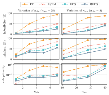
Figure 5: Performance evaluation for infeasibility rate, misclassification rate and suboptimality of different network architectures, depending on the number of obstacles and horizon length. The REDS network outperforms the other architectures, particularly for a larger number of obstacles and a longer horizon. Suboptimality is shown in a logarithmic scale.

Besides improving the performance metrics, the REDS also provides the desired structural properties. A REDS network can be trained and evaluated with a variable number of obstacles and prediction horizon. In Tab. II, the generalization performance of REDS network is shown, i.e., it is evaluated for numbers of obstacles that were not present in the training data. Tab. II compares generalization for an interpolation and extrapolation of the number of obstacles and the prediction horizon. According to Tab. II, REDS generalizes well for samples out of the training data distribution for the number of obstacles and the horizon length.

	Training		Testing		Performance (%)
	$n_{\mathrm{obs}}$	$N$	$n_{\mathrm{obs}}$	$N$	misclass.	infeas.	subopt.
	Generalization for the number of obstacles: interpolation
No general.	1-5	28	3	28	41.7	19.7	17.4
General.	1,2,4,5	28	3	28	42.0	19.8	11.6
	Generalization for the number of obstacles: extrapolation
No general.	1-5	28	5	28	30.3	24.4	3.9
General.	1-4	28	5	28	34.4	26.5	3.4
	Generalization for the horizon length
No general.	1-3	16	1-3	16	20.4	8.9	38.1
General.	1-3	12	1-3	16	26.0	10.8	20.9

TABLE II: Evaluation of the REDS network generalization performance (highlighted in bold).

VIII-B Evaluation for Ensemble of REDS Networks

In Fig. 6, we show the achieved feasibility rate on the test data using an ensemble with $n_{\mathrm{e}}=10$ REDS networks. In total, $2\cdot 10^{3}$ samples are evaluated for each NN individually and cumulatively. The performance improves by adding more NNs, however, also the total computation time increases. The parallel computation time results in the maximum time over the individual networks.

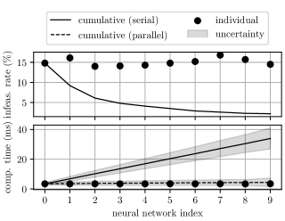
Figure 6: Individual and cumulative REDS prediction performance (infeasibility rate) and computation time concerning the number of NNs used in the ensemble. The computation time differs for parallel and serial evaluation. For the parallel evaluation, the slowest network determines the computation time.

Tab. III shows the memory usage and the number of parameters for the different architectures. The sizes of the networks are feasible for embedded devices [4], i.e., the REDS and EDS provide improved performance with a comparable or even reduced memory footprint than FFs and LSTMs. This may be due to exploiting the structure of equivariances and invariances inherently occurring in the application. Similar observations were made in other applications where deep sets have been applied, e.g., [18].

	FF	LSTM	EDS	REDS
Memory usage (MB)	2.40	0.97	0.51	1.40
Number of parameters ($10^{5}$)	5.98	2.41	1.26	3.43

TABLE III: Memory usage and number of parameters in NN architectures involving five obstacles and a horizon of 28 steps.

VIII-C Evaluation of REDS Planner with Feasibility Projection

Figure 7: Open-loop comparison of infeasibility rate and suboptimality of the REDS planner, using the QP without slack variables and the soft-QP followed by the FP. Infeasible problems are not considered in the suboptimality.

The REDS planner is validated on random samples of the test data, i.e., samples of the same distribution as the NN training data. Fig. 7 shows the infeasibility rate and suboptimality (7) of the REDS planner, using either the QP without slack variables, or the soft-QP followed by the FP. For an ensemble of ten NNs, the infeasibility rate of the QP without slack variables is below $10\%$ and decreased to almost $0\%$ by using the soft-QP followed by the FP, and the suboptimality is also negligible. The suboptimality of the soft-QP followed by the FP is higher than the suboptimality of the QP, since also infeasible problems are rendered feasible, yet with increased suboptimality values. Fig. 8 shows box plots of the computation times related to the different components. The main contributions to the total computation time of the REDS planner stem from the soft-QP (median of $\sim 4.2$ms) and the NNs (median of $\sim 3.0$ms per network). While the parallel architecture with ten NNs, as well as a single NN, decrease the worst case MIQP computation time by a factor of approximately $50$ and the median by a factor of $10$, the serial approach decreases the maximum by a factor of $8$ and the median by a factor of $2$. Besides computation time, the REDS planner is suitable for embedded system implementation as opposed to high-performance commercial solvers like the one used here as an expert, i.e., gurobi [11].

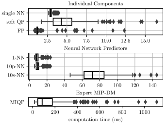
Figure 8: Box plots for open-loop comparison of the computation times of $10^{3}$ samples. REDS planner with an ensemble of one (1-NN) or ten NNs is parallelized (10p) or serial (10s).

IX Closed-loop Validations with SUMO Simulator

The following closed-loop evaluations of the REDS planner on a multi-lane highway scenario yield a more realistic performance measure. This involves challenges such as the distribution shift of the input parameters, wrong predictions and errors of the reference tracking NMPC.

IX-A Setup for Closed-loop Simulations

Several choices need to be made for parameters in the REDS planner and in the simulation environment.

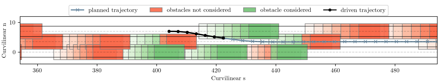
Figure 9: Obstacles considered at each planning step in the Frenet coordinate frame. The plot shows the ego point-mass trajectory and the inflated obstacles in proximity to the ego vehicle for seven time steps. The obstacle color indicates whether it was considered in planning or not.

IX-A1 Collision avoidance

For an environment with a large number of obstacles, we implement the following heuristic to select up to $n_{\mathrm{obs}}=5$ obstacles in proximity to the ego vehicle. We consider the closest successive obstacles in each lane that is not the lane of the ego vehicle and the leading vehicle on the ego lane. In Fig. 9, the selection of obstacles in proximity to the ego vehicle is shown in the Frenet coordinate frame. Obstacles are plotted in consecutive planner time steps, and the color indicates whether they are considered at each time step. Overtaking is allowed on both sides of a leading vehicle.

IX-A2 Sampling frequency

The planning frequency is set to $5$Hz, the control and ego vehicle simulation rate is $50$Hz and the SUMO simulation is $10$Hz. The traffic simulator in SUMO is slower than the ego vehicle simulation frequency, therefore the motion of the vehicles is linearly extrapolated between SUMO updates. Indeed, the REDS planner is real-time capable for selected frequencies, see Req. II.4.

IX-A3 Vehicle models

We use parameters of a BMW 320i for the ego vehicle, which is a medium-sized passenger vehicle whose parameters are provided in CommonRoad [14] for models of different fidelity. An odeint integrator of scipy simulates the $29$-state multi-body model [14] with a $20$ms time step. The traffic simulator SUMO [13] simulates interactive driving behaviors with the Krauss model [61] for car following and the LC2013 [62] model for lane changing. From zero up to five surrounding vehicles are selected for our comparisons.

IX-A4 Road layout

Standardized scenarios on German roads, provided by the scenario database of CommonRoad, are fully randomized before each closed-loop simulation, including the start configuration of the ego vehicle and all other vehicles. This initial randomization, in addition to the interactive and stochastic behavior simulated in SUMO, covers a wide range of traffic situations, including traffic jams, blocked lanes and irrational driver decisions such as half-completed lane changes. The basis of our evaluations is the three-lane scenario DEU_Cologne-63_5_I-1 with all (dense) or only a fourth (sparse) of the vehicles in the database.

IX-B Distribution Shift

The generally unknown state distribution encountered during closed-loop simulations, referred to as simulation distribution (SD), differs from the training distribution (TD). We aim to generalize with the proposed approach to a wide range of scenarios, hence, we use the uniform distribution given in Tab. VII to train the NNs and in consecutive closed-loop evaluations. However, if the encountered SD is known better, we propose to include NNs trained on an a priori known SD and include it in the ensemble of NNs. In Fig. 10, the worse performance of an ensemble of REDS, purely trained on the uniform TD, followed by the soft-QP is shown when evaluated for samples taken from closed-loop simulations of the DEU_Cologne-63_5_I-1 scenario using the expert MIP-DM. Additionally, Fig. 10 shows NNs trained on this SD and how they can improve the prediction performance as single networks by $\sim 10\%$ and in an ensemble by $\sim 3\%$.

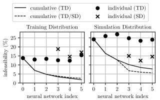
Figure 10: Individual and cumulative REDS prediction performance for the training distribution (TD) and samples encountered by an simulation distribution (SD). Two variants of the REDS ensemble are compared: one purely trained on the uniform training distribution (TD) and one ensemble with three NNs trained on the SD.

IX-C Closed-loop Results with SUMO Simulator

We compare the closed-loop performance of the REDS planner with varying numbers of NNs and of the expert MIP-DM for the dense and sparse traffic in scenario DEU_Cologne-63_5_I-1, c.f., Fig. 11. The closed-loop cost is computed by evaluating the objective (2) for the closed-loop trajectory and is separated into its components. The computation times are shown for the serial and parallel evaluation of the NNs. Similar to the open-loop evaluation in Fig. 6, the closed-loop results in Fig. 11 show a considerable performance gain when more NNs are added to the ensemble. Evaluating $10$ NNs in parallel within the REDS planner leads to nearly the same closed-loop performance as the expert MIP-DM. Remarkably, a parallel computation achieves a tremendous speed-up of the worst-case computation time of approximately $100$ times. A serial evaluation of $10$ NNs could still be computed around $25$ times faster for the maximum computation time compared to the expert MIP-DM. All computation times of the REDS planner variations are below the threshold of $200$ms, while the expert MIP-DM computation time exceeds the threshold in more than $50\%$, taking up to $4$s for one iteration.

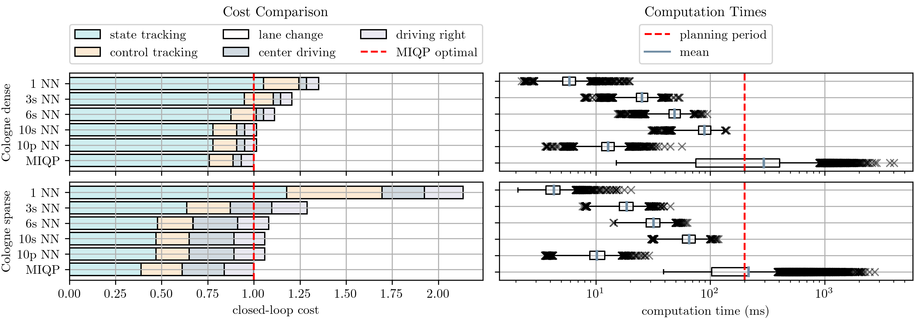
Figure 11: Performance comparison for different numbers of serial (s) and parallel (p) NNs, for dense and sparse traffic in scenario DEU_Cologne-63_5_I-1. The closed-loop cost was computed by evaluating (2) for the closed-loop ego trajectory and normalized against the closed-loop cost of expert MIP-DM. The state tracking cost, including the lateral position and the desired velocity tracking error, contributes the most to the chosen weights.

Tab. IV shows further performance metrics. By using more NNs within an ensemble increases the average velocity and decreases the closed-loop cost towards the expert MIP-DM performance. Using six or ten NNs, a single situation occurred where a leading vehicle started to change lanes but halfway decided to change back towards the original lane, resulting in a collision, which in a real situation will be avoided by an emergency (braking) maneuver. Fig. 12 shows snapshots of a randomized closed-loop SUMO simulation of a dense and sparse traffic scenario DEU_Cologne-63_5_I-1. The green colored ego vehicle successfully plans lane changes and overtaking maneuvers to avoid collisions with other vehicles (blue), using the proposed REDS planner feeding a reference tracking NMPC.

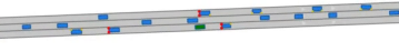
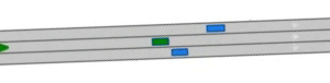
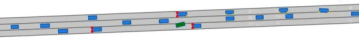
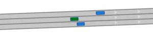
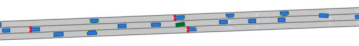
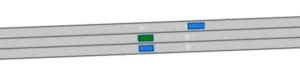
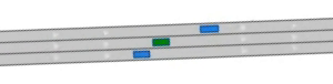
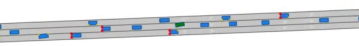
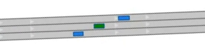
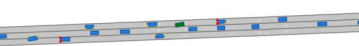
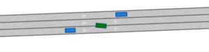
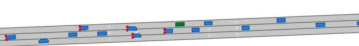
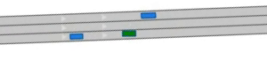
Figure 12: Snapshots of simulated traffic scenario DEU_Cologne-63_5_I-1 dense (left) and sparse (right) with SUMO and CommonRoad, showing the ego vehicle (green) and other vehicles (blue). The REDS planner is real-time feasible and used in combination with reference tracking NMPC, see Fig. 2. Red light at the rear of the vehicle indicate braking.

		DEU_Cologne-63_5_I-1-dense
Property	Unit	MIQP	NN-1	NN-3	NN-6	NN-10
collisions		0	0	0	1	1
vel. mean	$\frac{m}{s}$	13.10	12.71	12.91	13.00	13.07
vel. min	$\frac{m}{s}$	0.41	1.17	0.00	0.00	0.00
lane changes		457	431	469	471	462
cost	$\frac{1}{s}$	49.48	66.89	59.68	55.02	50.22
		DEU_Cologne-63_5_I-1-sparse
Property	Unit	MIQP	NN-1	NN-3	NN-6	NN-10
collisions		0	0	0	0	0
vel. mean	$\frac{m}{s}$	13.94	13.69	13.83	13.87	13.89
vel. min	$\frac{m}{s}$	7.10	7.10	7.10	7.10	7.10
lane changes		354	337	337	353	353
cost	$\frac{1}{s}$	5.81	12.40	7.49	6.27	6.16

TABLE IV: Closed-loop evaluation for scenario DEU_Cologne-63_5_I-1 with dense and sparse traffic.

X Conclusions and Discussion

We proposed a supervised learning approach for achieving real-time feasibility for mixed-integer motion planning problems. Several concepts are introduced to achieve a nearly optimal closed-loop performance when compared to an expert MIQP planner. First, it was shown that inducing structural problem properties such as invariance, equivariance and recurrence into the NN architecture improves the prediction performance among other useful properties such as generalization to unseen data. Secondly, the soft-QP can correct wrong predictions, inevitably linked to the NN predictions and are able to evaluate an open-loop cost. This favors a parallel architecture of an ensemble of predictions and soft-QP computations to choose the lowest-cost trajectory. In our experiments, adding NN to the ensemble improved the performance considerably and monotonously. This leads to the conclusion that NNs may be added as long as the computation time is below the planning threshold and as long as parallel resources are available. To further promote safety, an NLP, i.e., the FP, is used to plan a collision-free trajectory. The computational burden of the NLP is small, compared to the expert MIP-DM since it optimizes the trajectory only locally and therefore, omits the combinatorial variables.

Although we have evaluated the proposed approach for multi-lane traffic, the application to other urban driving scenarios is expected to perform similarly for a similar number of problem parameters due to the following. Many works, e.g., [22, 23, 6], use similar MIQP formulations for a variety of AD scenarios, including traffic lights, blocked lanes and merging. The formulations mainly differ in the specific environment. Many scenario specifics can be modeled by using obstacles and constraints related to the current lane [6], both considered in the presented approach. However, with an increasing number of problem parameters and rare events, the prediction of binary variables may become more challenging.

Rudolf Reiter received his Master’s degree in 2016 in electrical engineering with a focus on control systems from the Graz University of Technology, Austria. From 2016 to 2018 he worked as a Control Systems Specialist at the Anton Paar GmbH, Graz, Austria. From 2018 to 2021 he worked as a researcher for the Virtual Vehicle Research Center, in Graz, Austria, where he started his Ph.D. in 2020 under the supervision of Prof. Dr. Mortiz Diehl. Since 2021, he continued his Ph.D. at a Marie-Skłodowska Curie Innovative Training Network position at the University of Freiburg, Germany. His research focus is within the field of learning- and optimization-based motion planning and control for autonomous vehicles and he is an active member of the Autonomous Racing Graz team.

Rien Quirynen received the Bachelor’s degree in computer science and electrical engineering and the Master’s degree in mathematical engineering from KU Leuven, Belgium. He received a four-year Ph.D. Scholarship from the Research Foundation–Flanders (FWO) in 2012-2016, and the joint Ph.D. degree from KU Leuven, Belgium and the University of Freiburg, Germany. He worked as a senior research scientist at Mitsubishi Electric Research Laboratories in Cambridge, MA, USA from early 2017 until late 2023. Currently, he is a staff software engineer at Stack AV. His research focuses on numerical optimization algorithms for decision making, motion planning and predictive control of autonomous systems. He has authored/coauthored more than 75 peer-reviewed papers in journals and conference proceedings and 25 patents. Dr. Quirynen serves as an Associate Editor for the Wiley journal of Optimal Control Applications and Methods and for the IEEE CCTA Editorial Board.

Moritz Diehl studied mathematics and physics at Heidelberg University, Germany and Cambridge University, U.K., and received the Ph.D. degree in optimization and nonlinear model predictive control from the Interdisciplinary Center for Scientific Computing, Heidelberg University, in 2001. From 2006 to 2013, he was a professor with the Department of Electrical Engineering, KU Leuven University Belgium. Since 2013, he is a professor at the University of Freiburg, Germany, where he heads the Systems Control and Optimization Laboratory, Department of Microsystems Engineering (IMTEK), and is also with the Department of Mathematics. His research interests include optimization and control, spanning from numerical method development to applications in different branches of engineering, with a focus on embedded and on renewable energy systems.

Stefano Di Cairano received the Master’s (Laurea) and the Ph.D. degrees in information engineering in 2004 and 2008, respectively, from the University of Siena, Italy. During 2008-2011, he was with Powertrain Control R&A, Ford Research and Advanced Engineering, Dearborn, MI, USA. Since 2011, he is with Mitsubishi Electric Research Laboratories, Cambridge, MA, USA, where he is currently a Deputy Director, and a Distinguished Research Scientist. His research focuses on optimization-based control and decision-making strategies for complex mechatronic systems, in automotive, factory automation, transportation systems, and aerospace. His research interests include model predictive control, constrained control, path planning, hybrid systems, optimization, and particle filtering. He has authored/coauthored more than 200 peer-reviewed papers in journals and conference proceedings and 70 patents. Dr. Di Cairano was the Chair of the IEEE CSS Technical Committee on Automotive Controls and of the IEEE CSS Standing Committee on Standards. He is the inaugural Chair of the IEEE CCTA Editorial Board and was an Associate Editor of the IEEE Transactions on Control Systems Technology.

In the following, we define the most important parameters used in the numerical simulations of this paper. For the closed-loop simulations in SUMO, we used the parameter values in Tab. V. The reference velocity was set higher than the average nominal velocity to cause more overtaking maneuvers. For the optimization problems, we used the parameters shown in Tab. VI, in addition to the values presented in Tab. I. In Tab. VIII, neural network hyperparameters are shown for architectures FF, LSTM, EDS and REDS. The same LSTM layer is used for each set element (i.e., for each obstacle in our case) to achieve equivariance in the REDS network.

Category	Parameter	Value
General	episode length	$30$s
	nominal road velocity	$13.9\frac{\mathrm{m}}{\mathrm{s}}$
	maximum number of lanes	3
	lanes width $d_{\mathrm{lane}}$	$3.5$m
	vehicle lengths	$5.39$m
	vehicle widths	$2.07$m
	ego desired velocity	$15\frac{\mathrm{m}}{\mathrm{s}}$
	maximum obstacle velocity	$23\frac{\mathrm{m}}{\mathrm{s}}$
	minimum obstacle velocity	$0.2\frac{\mathrm{m}}{\mathrm{s}}$
Dense scenario	traffic flow	$0.56\frac{\mathrm{vehicles}}{\mathrm{lane}\cdot\mathrm{s}}$
	traffic density	$0.04\frac{\mathrm{vehicles}}{\mathrm{lane}\cdot\mathrm{m}}$
Sparse scenario	traffic flow	$0.13\frac{\mathrm{vehicles}}{\mathrm{lane}\cdot\mathrm{s}}$
	traffic density	$0.01\frac{\mathrm{vehicles}}{\mathrm{lane}\cdot\mathrm{m}}$
FP	diag$(Q)$	$[1,1,1,1]^{\top}$
	diag$(R)$	$[1,1]^{\top}$
	slack weight $w_{\mathrm{h}}$	$10^{6}$

TABLE V: Parameters for closed-loop simulations in SUMO.

Category	Parameter	Value
expert MIP-DM	diag$(Q)$	$[0,14,10,1]^{\top}$
	diag$(R)$	$[4,0.5]^{\top}$
	lane change weight $w_{\mathrm{lc}}$	$3\cdot 10^{3}$
	side preference weight $w_{\mathrm{rght}}$	$3$
	safe distances $[\sigma_{\mathrm{f}},\sigma_{\mathrm{b}},\sigma_{\mathrm{l}},\sigma_{\mathrm{r}}]^{\top}$	$[0.5,12,0.5,0.5]^{\top}$m
	minimum controls $\underline{u}$	$[\text{-}10,\text{-}5]^{\top}\frac{\mathrm{m}}{\mathrm{s}}$
	maximum controls $\overline{u}$	$[3,5]^{\top}\frac{\mathrm{m}}{\mathrm{s}}$
	velocity ratio constraint $\alpha$	$0.3$

TABLE VI: Parameters in MIQP formulation (III-C) for expert MIP-DM.

Par.	Range	Par.	Range
lat. pos.	$[0,n_{\mathrm{lanes}}d_{\mathrm{lanes}}]-\frac{d_{\mathrm{lanes}}}{2}$	lanes	[1,3]
obs. lon. pos.	$[\text{-}120,200]\mathrm{m}$	lon. vel.	$[0,30]\frac{\mathrm{m}}{\mathrm{s}}$
lat. vel.	$[\text{-}1,1]\frac{\mathrm{m}}{\mathrm{s}}$	obstacles	[1,5]

TABLE VII: Ranges of uniform training data distributions.

Category	Parameter	Value
General	activation function	ReLU
	batch size	$128$
	step size	$5\cdot 10^{\text{-}5}$
	epochs	$1500$
	optimizer	adam
	loss function	cross-entropy
	weight decay	$10^{-5}$
	training samples	$10^{5}$
	test samples	$10^{3}$
FF	hidden layers	$7$
	neurons per layer	$128$
LSTM	layers	$2$
	hidden network size	$128$
	input network layers	$2$
	output network layers	$2$
EDS	layers	$7$
	equivariant hidden size	$64$
	unstructured hidden size	$64$
	input network layers	$2$
	input network hidden size	$128$
	output network layers	$2$
	output network hidden size	$128$
REDS	layers	$7$
	hidden network sizes	$64$
	input network layers	$1$
	output network layers	$1$
	eq. LSTM output network layers	$1$
	unstr. LSTM output network layers	$1$

TABLE VIII: Hyperparameters for the NN architectures.

References

- [1] B. Paden, M. Čáp, S. Z. Yong, D. Yershov, and E. Frazzoli, “A survey of motion planning and control techniques for self-driving urban vehicles,” IEEE Transactions on Intelligent Vehicles, vol. 1, no. 1, pp. 33–55, 2016.
- [2] J. H. Reif, “Complexity of the mover’s problem and generalizations,” in 20th Annual Symposium on Foundations of Computer Science (sfcs 1979), 1979, pp. 421–427.
- [3] S. M. LaValle, Planning Algorithms. USA: Cambridge University Press, 2006.
- [4] S. Di Cairano and I. V. Kolmanovsky, “Real-time optimization and model predictive control for aerospace and automotive applications,” ser. Amer. Control Conf., 2018, pp. 2392–2409.
- [5] J. Guanetti, Y. Kim, and F. Borrelli, “Control of connected and automated vehicles: State of the art and future challenges,” Annual Reviews in Control, vol. 45, pp. 18 – 40, 2018.
- [6] R. Quirynen, S. Safaoui, and S. Di Cairano, “Real-time mixed-integer quadratic programming for vehicle decision making and motion planning,” ArXiv, 2023.
- [7] A. Cauligi, P. Culbertson, E. Schmerling, M. Schwager, B. Stellato, and M. Pavone, “CoCo: Online mixed-integer control via supervised learning,” IEEE Robotics and Automation Letters, vol. 7, no. 2, pp. 1447–1454, 2022.
- [8] D. Bertsimas and B. Stellato, “The voice of optimization,” Machine Learning, vol. 110, no. 2, pp. 249–277, Feb. 2021.
- [9] R. Verschueren, G. Frison, D. Kouzoupis, J. Frey, N. van Duijkeren, A. Zanelli, B. Novoselnik, T. Albin, R. Quirynen, and M. Diehl, “acados – a modular open-source framework for fast embedded optimal control,” Mathematical Programming Computation, Oct 2021.
- [10] Q. Tran Dinh, S. Gumussoy, W. Michiels, and M. Diehl, “Combining convex–concave decompositions and linearization approaches for solving bmis, with application to static output feedback,” IEEE Transactions on Automatic Control, vol. 57, no. 6, pp. 1377–1390, 2012.
- [11] Gurobi Optimization, LLC, “Gurobi Optimizer Reference Manual,” 2023. [Online]. Available: https://www.gurobi.com
- [12] A. Cauligi, A. Chakrabarty, S. Di Cairano, and R. Quirynen, “Prism: Recurrent neural networks and presolve methods for fast mixed-integer optimal control,” in Proceedings of The 4th Annual Learning for Dynamics and Control Conference, ser. Proceedings of Machine Learning Research, vol. 168. PMLR, 23–24 Jun 2022, pp. 34–46.
- [13] P. A. Lopez, M. Behrisch, L. Bieker-Walz, J. Erdmann, Y.-P. Flötteröd, R. Hilbrich, L. Lücken, J. Rummel, P. Wagner, and E. Wießner, “Microscopic traffic simulation using SUMO,” in The 21st IEEE International Conference on Intelligent Transportation Systems. IEEE, 2018.
- [14] M. Althoff, M. Koschi, and S. Manzinger, “Commonroad: Composable benchmarks for motion planning on roads,” in 2017 IEEE Intelligent Vehicles Symposium (IV), 2017, pp. 719–726.
- [15] C. Xi, T. Shi, Y. Wu, and L. Sun, “Efficient motion planning for automated lane change based on imitation learning and mixed-integer optimization,” in IEEE 23rd International Conference on Intelligent Transportation Systems (ITSC), 2020, pp. 1–6.
- [16] M. Srinivasan, A. Chakrabarty, R. Quirynen, N. Yoshikawa, T. Mariyama, and S. Di. Cairano, “Fast multi-robot motion planning via imitation learning of mixed-integer programs,” IFAC-PapersOnLine, vol. 54, no. 20, pp. 598–604, 2021, modeling, Estimation and Control Conference MECC.
- [17] S. Aradi, “Survey of deep reinforcement learning for motion planning of autonomous vehicles,” IEEE Transactions on Intelligent Transportation Systems, vol. 23, no. 2, pp. 740–759, 2022.
- [18] M. Huegle, G. Kalweit, B. Mirchevska, M. Werling, and J. Boedecker, “Dynamic input for deep reinforcement learning in autonomous driving,” in IEEE/RSJ International Conference on Intelligent Robots and Systems (IROS), 2019, pp. 7566–7573.
- [19] J. Park, S. Karumanchi, and K. Iagnemma, “Homotopy-based divide-and-conquer strategy for optimal trajectory planning via mixed-integer programming,” IEEE Transactions on Robotics, vol. 31, no. 5, pp. 1101–1115, 2015.
- [20] X. Qian, F. Altché, P. Bender, C. Stiller, and A. de La Fortelle, “Optimal trajectory planning for autonomous driving integrating logical constraints: An miqp perspective,” in IEEE 19th International Conference on Intelligent Transportation Systems (ITSC), 2016, pp. 205–210.
- [21] K. Esterle, T. Kessler, and A. Knoll, “Optimal behavior planning for autonomous driving: A generic mixed-integer formulation,” in IEEE Intelligent Vehicles Symposium (IV), 2020, pp. 1914–1921.
- [22] T. Kessler, K. Esterle, and A. Knoll, “Linear differential games for cooperative behavior planning of autonomous vehicles using mixed-integer programming,” in 59th IEEE Conference on Decision and Control (CDC), 2020, pp. 4060–4066.
- [23] ——, “Mixed-integer motion planning on german roads within the apollo driving stack,” IEEE Transactions on Intelligent Vehicles, vol. 8, no. 1, pp. 851–867, 2023.
- [24] R. Reiter, M. Kirchengast, D. Watzenig, and M. Diehl, “Mixed-integer optimization-based planning for autonomous racing with obstacles and rewards,” IFAC-PapersOnLine, vol. 54, no. 6, pp. 99–106, 2021, 7th IFAC Conference on Nonlinear Model Predictive Control NMPC.
- [25] L. Russo, S. H. Nair, L. Glielmo, and F. Borrelli, “Learning for online mixed-integer model predictive control with parametric optimality certificates,” IEEE Control Systems Letters, vol. 7, pp. 2215–2220, 2023.
- [26] D. Bertsimas and B. Stellato, “Online mixed-integer optimization in milliseconds,” INFORMS J. on Computing, vol. 34, no. 4, p. 2229–2248, jul 2022.
- [27] D. Masti and A. Bemporad, “Learning binary warm starts for multiparametric mixed-integer quadratic programming,” in 18th European Control Conference (ECC), 2019, pp. 1494–1499.
- [28] V. Nair, S. Bartunov, F. Gimeno, I. von Glehn, P. Lichocki, I. Lobov, B. O’Donoghue, N. Sonnerat, C. Tjandraatmadja, P. Wang, R. Addanki, T. Hapuarachchi, T. Keck, J. Keeling, P. Kohli, I. Ktena, Y. Li, O. Vinyals, and Y. Zwols, “Solving mixed integer programs using neural networks,” ArXiv, vol. abs/2012.13349, 2020.
- [29] E. B. Khalil, C. Morris, and A. Lodi, “MIP-GNN: A data-driven framework for guiding combinatorial solvers,” in Proceedings of the 36th AAAI Conference on Artificial Intelligence, 2022.
- [30] F. Eiras, M. Hawasly, S. V. Albrecht, and S. Ramamoorthy, “A two-stage optimization-based motion planner for safe urban driving,” IEEE Transactions on Robotics, vol. 38, no. 2, pp. 822–834, 2022.
- [31] L. Claussmann, M. Revilloud, D. Gruyer, and S. Glaser, “A review of motion planning for highway autonomous driving,” IEEE Transactions on Intelligent Transportation Systems, vol. 21, no. 5, pp. 1826–1848, 2020.
- [32] M. Reda, A. Onsy, A. Y. Haikal, and A. Ghanbari, “Path planning algorithms in the autonomous driving system: A comprehensive review,” Robotics and Autonomous Systems, vol. 174, p. 104630, 2024.
- [33] M. Sheckells, T. M. Caldwell, and M. Kobilarov, “Fast approximate path coordinate motion primitives for autonomous driving,” in IEEE 56th Annual Conference on Decision and Control (CDC), 2017, pp. 837–842.
- [34] L. Kavraki, P. Svestka, J.-C. Latombe, and M. Overmars, “Probabilistic roadmaps for path planning in high-dimensional configuration spaces,” IEEE Transactions on Robotics and Automation, vol. 12, no. 4, pp. 566–580, 1996.
- [35] O. Arslan, K. Berntorp, and P. Tsiotras, “Sampling-based algorithms for optimal motion planning using closed-loop prediction,” in IEEE International Conference on Robotics and Automation (ICRA), 2017, pp. 4991–4996.
- [36] Z. Ajanovic, B. Lacevic, B. Shyrokau, M. Stolz, and M. Horn, “Search-based optimal motion planning for automated driving,” in IEEE/RSJ International Conference on Intelligent Robots and Systems (IROS), 2018, pp. 4523–4530.
- [37] P. Bender, O. S. Tas, J. Ziegler, and C. Stiller, “The combinatorial aspect of motion planning: Maneuver variants in structured environments,” in IEEE Intelligent Vehicles Symposium (IV), 2015, pp. 1386–1392.
- [38] C. Miller, C. Pek, and M. Althoff, “Efficient mixed-integer programming for longitudinal and lateral motion planning of autonomous vehicles,” in IEEE Intelligent Vehicles Symposium (IV), 2018, pp. 1954–1961.
- [39] J. Li, X. Xie, Q. Lin, J. He, and J. M. Dolan, “Motion planning by search in derivative space and convex optimization with enlarged solution space,” in IEEE/RSJ International Conference on Intelligent Robots and Systems (IROS), 2022, pp. 13 500–13 507.
- [40] S. Deolasee, Q. Lin, J. Li, and J. M. Dolan, “Spatio-temporal motion planning for autonomous vehicles with trapezoidal prism corridors and Bézier curves,” in American Control Conference, San Diego, CA, USA. IEEE, 2023, pp. 3207–3214.
- [41] M. Diehl, H. G. Bock, and J. P. Schlöder, “A real-time iteration scheme for nonlinear optimization in optimal feedback control,” SIAM Journal on Control and Optimization, vol. 43, no. 5, pp. 1714–1736, 2005.
- [42] H. Zhou, D. Ren, H. Xia, M. Fan, X. Yang, and H. Huang, “Ast-gnn: An attention-based spatio-temporal graph neural network for interaction-aware pedestrian trajectory prediction,” Neurocomputing, vol. 445, pp. 298–308, 2021.
- [43] E. Jo, M. Sunwoo, and M. Lee, “Vehicle trajectory prediction using hierarchical graph neural network for considering interaction among multimodal maneuvers,” Sensors, vol. 21, no. 16, 2021.
- [44] L. Brunke, M. Greeff, A. W. Hall, Z. Yuan, S. Zhou, J. Panerati, and A. P. Schoellig, “Safe learning in robotics: From learning-based control to safe reinforcement learning,” Annual Review of Control, Robotics, and Autonomous Systems, vol. 5, no. 1, pp. 411–444, 2022.
- [45] J. Van Brummelen, M. O’Brien, D. Gruyer, and H. Najjaran, “Autonomous vehicle perception: The technology of today and tomorrow,” Transportation Research Part C: Emerging Technologies, vol. 89, pp. 384–406, 2018.
- [46] T. Ersal, I. Kolmanovsky, N. Masoud, N. Ozay, J. Scruggs, R. Vasudevan, and G. Orosz, “Connected and automated road vehicles: state of the art and future challenges,” Vehicle system dynamics, vol. 58, no. 5, pp. 672–704, 2020.
- [47] K. Berntorp, A. Weiss, and S. Di Cairano, “Integer ambiguity resolution by mixture kalman filter for improved gnss precision,” IEEE Transactions on Aerospace and Electronic Systems, vol. 56, no. 4, pp. 3170–3181, 2020.
- [48] M. Greiff, S. Di Cairano, K. J. Kim, and K. Berntorp, “A system-level cooperative multiagent gnss positioning solution,” IEEE Transactions on Control Systems Technology, 2023.
- [49] M. Zaheer, S. Kottur, S. Ravanbakhsh, B. Poczos, R. R. Salakhutdinov, and A. J. Smola, “Deep sets,” in Advances in Neural Information Processing Systems, vol. 30. Curran Associates, Inc., 2017.
- [50] R. Reiter and M. Diehl, “Parameterization approach of the frenet transformation for model predictive control of autonomous vehicles,” in European Control Conference (ECC), 2021, pp. 2414–2419.
- [51] A. Vaswani, N. Shazeer, N. Parmar, J. Uszkoreit, L. Jones, A. N. Gomez, Ł. Kaiser, and I. Polosukhin, “Attention is all you need,” in Advances in neural information processing systems, 2017, pp. 5998–6008.
- [52] L. Hansen and P. Salamon, “Neural network ensembles,” IEEE Transactions on Pattern Analysis and Machine Intelligence, vol. 12, no. 10, pp. 993–1001, 1990.
- [53] P. Sollich and A. Krogh, “Learning with ensembles: How overfitting can be useful,” in Advances in Neural Information Processing Systems, vol. 8. MIT Press, 1995.
- [54] G. Frison and M. Diehl, “HPIPM: a high-performance quadratic programming framework for model predictive control,” IFAC-PapersOnLine, vol. 53, no. 2, pp. 6563–6569, 2020, 21st IFAC World Congress.
- [55] F. Debrouwere, W. Van Loock, G. Pipeleers, Q. T. Dinh, M. Diehl, J. De Schutter, and J. Swevers, “Time-optimal path following for robots with convex–concave constraints using sequential convex programming,” IEEE Transactions on Robotics, vol. 29, no. 6, pp. 1485–1495, 2013.
- [56] S. Gros, M. Zanon, R. Quirynen, A. Bemporad, and M. Diehl, “From linear to nonlinear MPC: bridging the gap via the real-time iteration,” International Journal of Control, vol. 93, no. 1, pp. 62–80, 2020.
- [57] J. Nocedal and S. J. Wright, Numerical Optimization, 2nd ed. New York, NY, USA: Springer, 2006.
- [58] S. Diamond and S. Boyd, “CVXPY: A Python-embedded modeling language for convex optimization,” Journal of Machine Learning Research, vol. 17, no. 83, pp. 1–5, 2016.
- [59] J. A. E. Andersson, J. Gillis, G. Horn, J. B. Rawlings, and M. Diehl, “CasADi – A software framework for nonlinear optimization and optimal control,” Mathematical Programming Computation, vol. 11, no. 1, pp. 1–36, 2019.
- [60] D. P. Kingma and J. Ba, “Adam: A method for stochastic optimization,” in 3rd International Conference on Learning Representations, ICLR, San Diego, CA, USA, May 7-9, 2015, Conference Track Proceedings, 2015.
- [61] S. Krauss, “Microscopic modeling of traffic flow: Investigation of collision free vehicle dynamics,” PhD thesis, University of Cologne, April 1998.
- [62] J. Erdmann, “SUMO’s lane-changing model,” in Modeling Mobility with Open Data, M. Behrisch and M. Weber, Eds. Cham: Springer International Publishing, 2015, pp. 105–123.