Modeling sea ice in the marginal ice zone as a dense granular flow with rheology inferred from a discrete element model

Abstract

The marginal ice zone (MIZ) represents the periphery of the sea ice cover. Here, the macroscale behavior of the sea ice results from collisions and enduring contact between ice floes. This configuration closely resembles that of dense granular flows, which have been modeled successfully with the $\mu(I)$ rheology. Here, we present a continuous model based on the $\mu(I)$ rheology which treats sea ice as a compressible fluid, with the local sea ice concentration given by a dilatancy function $\Phi(I)$. We infer expressions for $\mu(I)$ and $\Phi(I)$ from a discrete element method (DEM) which considers polygonal-shaped ice floes. We do this by driving the sea ice with a one-dimensional shearing ocean current. The resulting continuous model is a nonlinear system of equations with the sea ice velocity, local concentration, and pressure as unknowns. The rheology is given by the sum of a plastic and a viscous term. In the context of a periodic patch of ocean, which is effectively a one dimensional problem, and under steady conditions, we prove this system to be well-posed, present a numerical algorithm for solving it, and compare its solutions to those of the DEM. These comparisons demonstrate the continuous model’s ability to capture most of the DEM’s results accurately. The continuous model is particularly accurate for ocean currents faster than 0.25 m/s; however, for low concentrations and slow ocean currents, the continuous model is less effective in capturing the DEM results. In the latter case, the lack of accuracy of the continuous model is found to be accompanied by the breakdown of a balance between the average shear stress and the integrated ocean drag extracted from the DEM. Since this balance is expected to hold independently of our choice of rheology, this finding indicates that continuous models might not be able to describe sea ice dynamics for low concentrations and slow ocean currents.

1 Introduction

The periphery of the ice cover is known as the marginal ice zone (MIZ)and consists of relatively small, typically polygon-shaped ice floes. It is often defined as the region where ocean waves play an important role in shaping the morphological properties of the ice (Dumont,, 2022). On large scales, sea ice dynamics are typically described with Hibler’s model (Hibler III,, 1979), which treats ice as a viscoplastic fluid whose yield strength depends on the sea ice concentration and thickness. This model was developed for the central ice pack, where ice floes are closely interlocked and deformation is mostly due to the opening of leads or the formation of ridges.

In the MIZ, however, it is the collisions and enduring contact between ice floes that give rise to the macroscale dynamical properties of the ice cover (Feltham,, 2005; Herman,, 2011, 2022). This configuration closely resembles that of dense granular flows, albeit at different spatial scales, since practically all studies for granular materials consider e.g. polystyrene beads, glass beads, and sand, whose particles’ diameters are in the order of 0.1 and 1 mm (MiDi,, 2004). Dense granular flows have been successfully modeled with the so-called $\mu(I)$ rheology (Da Cruz et al.,, 2005). The dense granular flow regime is understood as a transition between the quasi-static and dilute flow regimes. Whenever grain inertia is negligible, a quasi-static regime emerges which is often modeled as an elastoplastic solid (Nedderman,, 1992). The critical state at which plastic deformation occurs is characterized with a Coulomb-like criterion dependent on a so-called internal angle of friction (Wood,, 1990). Conversely, under great agitation and/or dilute concentrations of grains, particles interact only through binary, instantaneous, uncorrelated collisions. As a result, ideas from kinetic theory become applicable in this dilute regime (Jenkins and Savage,, 1983). However, in dense granular flows, grains interact via collisions and enduring contacts, such that inertial effects are important yet the collisions may no longer be assumed to be binary, instantaneous, or uncorrelated in general. This transitional regime is characterized in terms of the inertial number $I$ and an effective friction coefficient $\mu$ depedent on $I$ (Da Cruz et al.,, 2005).

Existing models for the MIZ recognize the importance of both collisions and plastic deformation, and derive rheological models based on first principles (Shen et al.,, 1987; Gutfraind and Savage,, 1997; Feltham,, 2005). Recently, Herman, (2022) suggests the use of the $\mu(I)$ rheology for modeling sea ice in the MIZ and derives a $\mu(I)$ function from computations performed with a discrete element method (DEM). In these computations, disk-shaped ice floes are sheared by a moving wall in the classical manner of rheological studies. Unlike the previous models for the MIZ, Herman, (2022) infers the rheological properties from data generated by a DEM. In particular, Herman, (2022) fits a $\mu(I)$ function to the DEM’s data, although the resulting continuous model and its accuracy in replicating the DEM’s results is not examined.

This work represents an advance in the development of a continuous model for the MIZ that could improve the accuracy of Hibler’s model, which is currently used in large-scale climate models over the MIZ, see for example (Danabasoglu et al.,, 2020). A comparison of Hibler’s model with the DEM data is presented in section 6.1, where it is demonstrated that it cannot capture the DEM results accurately. We extend the investigation initiated in Herman, (2022) and explore the $\mu(I)$ rheology’s accuracy in modeling sea ice dynamics in the MIZ. We infer a $\mu(I)$ function from computations performed with the DEM implemented in SubZero (Manucharyan and Montemuro,, 2022). This DEM considers polygon-shaped ice floes that are driven by oceanic currents in an open patch of ocean, a setup which we believe to be more natural for studying sea ice than the classical shearing test with a moving wall and disk-shaped ice floes. This inference results in a continuous viscous fluid model whose rheology is given by the sum of a viscous and a plastic term. Moreover, for this system to be well-posed, the emerging continuous model problem requires the continuum to be compressible and complemented with a constraint on the global sea ice concentration. Assuming the continuum to be compressible requires the inference of a dilatancy function $\Phi(I)$ from the DEM computations which establishes a relationship between local sea ice concentration and the inertial number $I$.

The contributions of this paper can be summarized as follows: (1) Inference of the $\mu(I)$ and $\Phi(I)$ constitutive functions for sea ice in the MIZ from DEM computations performed in an open ocean configuration where the sea ice is sheared by ocean currents. (2) Analysis of the resulting continuous model, establishing the existence and uniqueness of solutions. (3) Determination of the continuous model’s range of validity by comparing its numerical solutions to those of the DEM.

We remark that the analysis of the continuous model and its comparisons with the DEM are restricted to a steady one dimensional setup. The model can be extended to unsteady two dimensional problems as explained in section 2.1, although we expect new complications will arise with these extensions. For example, Barker et al., (2015) demonstrates the emergence of time-dependent instabilities in $\mu(I)$ models. These potential complications should be studied carefully in future investigations.

This paper is structured as follows. In section 2, we formulate the continuous model, first in a general two-dimensional unsteady setting, then in the one dimensional steady configuration considered in this paper. In this formulation, two functions, $\mu(I)$ and $\Phi(I)$, are to be inferred from the DEM. This inference is presented in section 3. Section 4 contains a detailed analysis of the continuous model resulting from this inference. This analysis examines several properties of the momentum equation, the numerical solution of the continuous model, and its well-posedness. Then, in section 5, we compare the continuous model and the DEM. This comparison allows us to establish the range of validity of the numerical model and its limitations. In section 6, we discuss the similarities and differences between our continuous model and other sea ice models, such as Hibler’s model. We then end this paper with section 7, where we recommend potential extensions of this work to be explored in the future.

2 Mathematical formulation of the continuous problem

The dense flow regime represents a transition between the quasi-static and dilute flow regimes (Da Cruz et al.,, 2005). This transitional regime is characterized in terms of the inertial number $I$, an effective friction coefficient $\mu(I)$, and, whenever the continuum is assumed to be compressible, a dilatancy function $\Phi(I)$. Below, we define these three terms and present a general formulation of the $\mu(I)$ rheology in two dimensions and in the one dimensional steady configuration considered in the subsequent sections of this paper.

2.1 The two-dimensional setting

Although the problems presented in this paper are effectively one dimensional, we first present the general form of the flow model in two dimensions for completeness. We denote the ice velocity, concentration, and Cauchy stress tensor by $\boldsymbol{u}$, $A$, and $\boldsymbol{\sigma}$, respectively. We write the components of the Cauchy stress tensor and the velocity vector field as

$$\boldsymbol{\sigma}=\left[\begin{array}[]{cc}\sigma_{xx}&\sigma_{xy}\\ \sigma_{xy}&\sigma_{yy}\end{array}\right]\quad\text{and}\quad\boldsymbol{u}=(u,v),$$ (2.3)

respectively. We assume that the morphology of the ice floes remains invariant by neglecting all thermomechanical effects, such as fracturing, melting, or ridging, that can change the shape of a floe. For simplicity, we also neglect the Coriolis force, ocean tilting and the atmospheric drag (we assume low-wind conditions). Under these conditions, conservation of momentum and mass lead to the following system of equations:

$$\rho H\frac{\mathrm{D}\boldsymbol{u}}{\mathrm{D}t} =\nabla\cdot\boldsymbol{\sigma}+\boldsymbol{t}_{o},$$ (2.4a)

$$\frac{\mathrm{D}A}{\mathrm{D}t} =-A\,\nabla\cdot\boldsymbol{u}.$$ (2.4b)

see Hibler III, (1979) or Gray and Morland, (1994). For any scalar or vector-valued function $f$, the material derivative is given by $\mathrm{D}f/\mathrm{D}t=\partial f/\partial t+(\boldsymbol{u}\cdot\nabla)\,f$. Here, we assume the ice thickness $H$ to be spatially uniform for simplicity, although in general we require an additional equation, analogous to (2.4b) but in terms of $H$, for mass to be conserved. Equation (2.4a) is a depth-averaged statement of conservation of momentum of the sea ice layer; here, $\boldsymbol{t}_{o}$ is the drag force exerted by the ocean on the sea ice. Given the surface ocean velocity field $\boldsymbol{u}_{o}$, this drag force is generally parameterized in terms of the drag coefficient $C_{o}$ and the ocean water density $\rho_{o}$by

$$\boldsymbol{t}_{o}:=\rho_{o}C_{o}\|\boldsymbol{u}_{o}-\boldsymbol{u}\|(\boldsymbol{u}_{o}-\boldsymbol{u}),$$ (2.5)

with $\|\cdot\|$ denoting the Euclidean norm of a vector.

The conservation laws (2.4) must be accompanied by constitutive relations. To write these, we first decompose the Cauchy stress tensor into a pressure term $p$ and its deviatoric component $\boldsymbol{\tau}$,

$$\boldsymbol{\sigma}=\boldsymbol{\tau}-p\boldsymbol{\mathrm{I}},$$ (2.6)

where $\boldsymbol{\mathrm{I}}$ is the identity tensor, and define the strain rate tensor $\boldsymbol{\mathrm{D}}$ and its deviatoric component $\boldsymbol{\mathrm{S}}$ as

$$\boldsymbol{\mathrm{D}}:=\frac{1}{2}\left(\nabla\boldsymbol{u}+\nabla\boldsymbol{u}^{\top}\right)\quad\text{and}\quad\boldsymbol{\mathrm{S}}:=\boldsymbol{\mathrm{D}}-\frac{1}{2}\left(\nabla\cdot\boldsymbol{u}\right)\boldsymbol{\mathrm{I}}.$$ (2.7)

In the following, for a given tensor $\boldsymbol{\mathrm{T}}$, its second invariant is denoted by

$$\|\boldsymbol{\mathrm{T}}\|=\sqrt{\frac{1}{2}\operatorname{tr}{(\boldsymbol{\mathrm{T}}^{2})}}.$$ (2.8)

The fundamental idea behind the $\mu(I)$ rheology is that the constitutive relation for a granular flow depends on the inertial number, a dimensionless quantity defined as

$$I:=\overline{d}\sqrt{\frac{H\rho_{i}}{p}}\|\boldsymbol{\mathrm{S}}\|,$$ (2.9)

where $\rho_{i}$ is the ice density, $\overline{d}$ an average of the ice floe size, and $p$ the pressure emerging in (2.6) (Da Cruz et al.,, 2005; Jop et al.,, 2006; Pouliquen et al.,, 2006). Throughout this document, we set $\overline{d}$ to be spatially constant over the whole domain, avoiding the need to consider the transport of this quantity. Savage, (1984) interprets the quantity $I^{2}$ as the ratio between collisional (i.e. inertial) stresses and the total shear stress exerted on the material. Accordingly, for low values of $I$, the inertial effects of grains become negligible and the flow approaches a quasi-static regime; conversely, as $I$ increases, collisional forces become increasingly important relative to the external forces exerted on the material. The functional relationship that establishes the material’s rheology is written in terms of an effective friction $\mu(I)$, defined as

$$\mu(I):=\frac{\|\boldsymbol{\tau}\|}{p}.$$ (2.10)

We remark that the effective friction $\mu$ is defined in analogy with Coulomb’s model of friction as the ratio between the shear (tangential) stress and the pressure (normal stress). Moreover, it is also helpful to think of the pressure $p$ as a quantification of the material’s strength and its resistance to viscous and plastic deformation, as made clear in section 4.

To obtain a relationship between stress and strain, we need an additional constitutive law. Jop et al., (2006) propose the following equality that aligns $\boldsymbol{\mathrm{S}}$ with $\boldsymbol{\tau}$:

$$\frac{\boldsymbol{\mathrm{S}}}{\|\boldsymbol{\mathrm{S}}\|}=\frac{\boldsymbol{\tau}}{\|\boldsymbol{\tau}\|}.$$ (2.11)

Combining (2.10) and (2.11), the relationship between deviatoric components of the stress tensor and the shear strain can be written as

$$\boldsymbol{\tau}=\mu(I)p\frac{\boldsymbol{\mathrm{S}}}{\|\boldsymbol{\mathrm{S}}\|}.$$ (2.12)

Compressible granular flows require a dilatancy law which relates the concentration $A$ with the inertial number $I$,

$$A=\Phi(I),$$ (2.13)

see Da Cruz et al., (2005). In general, $\Phi$ is found to be a strictly decreasing function of $I$, in such a way that the concentration $A$ decreases with the rate of shearing $\|\boldsymbol{\mathrm{S}}\|$, a phenomenon know as dilatancy. Moreover, if $\Phi$ is strictly decreasing, it is invertible, and one can write an expression for the pressure $p$ analogous to an equation of state in thermodynamics,

$$p=\rho_{i}\overline{d}^{2}H\left(\frac{\|\boldsymbol{\mathrm{S}}\|}{\Phi^{-1}(A)}\right)^{2},$$ (2.14)

where we have combined equations (2.9) and (2.13). In the problems considered in this paper, we find the spatial variations in sea ice concentration to be small. Although this would make the assumption of incompressibility reasonable, the periodic one dimensional nature of these problems renders the dilatancy law (2.13) necessary for the model to be well-posed. This point is explained below in section 2.2.

2.2 The steady one dimensional periodic ocean problem

The model problem considered in this paper consists of a square patch of ocean of length $L$ with periodic boundaries in both the $x$ and $y$-directions. The ice floes floating on this patch are driven by an ocean velocity field that only varies in the $y$-direction, as depicted in figure 1. We neglect time-dependent effects and only consider steady conditions in the forcing i.e. $\boldsymbol{u}_{o}(x,y,t)=(u_{o}(y),0)$.

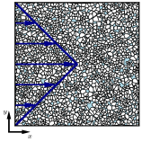
Figure 1: The periodic ocean setup. The domain is a square patch of ocean, periodic in the horizontal and vertical directions. The ice floes are driven by the ocean velocity field (2.17) (in blue), which does not vary in the $x$-direction.

This configuration renders the continuous problem one dimensional and independent of time, such that $\boldsymbol{u}(x,y,t)=(u(y),0)$, $A(x,y,t)=A(y)$, and $p(x,y,t)=p(y)$. In this setting, the equations for conservation of momentum (2.4a), together with the constitutive equation (2.12), simplify to the following system on $(0,L)$:

$$-\frac{\mathrm{d}\sigma_{xy}}{\mathrm{d}y}=\rho_{o}C_{o}|u_{o}-u|(u_{o}-u)$$ (2.15a)

$$\frac{\mathrm{d}p}{\mathrm{d}y}=0,$$ (2.15b)

$$\sigma_{xy}=\mu(I)p\frac{\mathrm{d}u/\mathrm{d}y}{\left|\mathrm{d}u/\mathrm{d}y\right|},$$ (2.15c)

$$I=\overline{d}\sqrt{\frac{H\rho_{i}}{p}}\left|\mathrm{d}u/\mathrm{d}y\right|.$$ (2.15d)

Due to (2.15b), which represents the balance of momentum in the $y$-direction, the pressure is a constant (but unknown) over the domain. Da Cruz et al., (2005) and Herman, (2022) find $p$ by enforcing normal stress boundary conditions along a boundary of the domain, but we cannot do the same because the domain is periodic. In the DEM computations, which we introduce in section 3, we set a global ice concentration $A_{0}\in[0,1]$ which equals the domain averaged value of the local concentration $A$, such that

$$\frac{1}{L}\int_{0}^{L}A\,\mathrm{d}y=A_{0}.$$ (2.16)

Therefore, if we assume the sea ice to behave like a compressible fluid, condition (2.16) and the dilatancy law (2.13) close the system of equations. In sections 3 and 5, we justify this modeling choice by demonstrating that dilatancy emerges in the DEM computations and that our model is capable of capturing it accurately.

In this paper we only consider the following ocean velocity profile for simplicity:

$$u_{o}(y)=u_{o,max}\left(1-|1-2y/L|\right),$$ (2.17)

for some maximum velocity $u_{o,max}>0$. Figure 1 contains a plot of this velocity profile.

3 Inferring the constitutive equations of the system from the DEM

$C_{o}$	$\rho_{i}$	$\rho_{o}$	$E$	$\nu$	$\mu^{\ast}$
$3\times 10^{-3}$	$900\,$\mathrm{k}\mathrm{g}$/$\mathrm{m}$^{3}$	$1026\,$\mathrm{k}\mathrm{g}$/$\mathrm{m}$^{3}$	$6\times 10^{6}\,$\mathrm{P}\mathrm{a}$$	0.3	0.2

Table 1: Values for material parameters used throughout this document. Here, $C_{o}$ is the drag coefficient for the ocean current and $\rho_{i}$ and $\rho_{o}$ are the ice and ocean water densities, respectively. The Young’s modulus $E$, Poisson’s ratio $\nu$, and inter-floe friction coefficient $\mu^{\ast}$ are used in the calculation of collisional forces, as described in Appendix A.1.

The system of equations presented in section 2.2 is incomplete because we need additional expressions for $\mu(I)$ and $\Phi(I)$. In this paper, we infer these additional equations from data generated with SubZero, a DEM developed by Manucharyan and Montemuro, (2022) and used for modeling sea ice dynamics with poylgonal-shaped ice floes. Following the setup presented in section 2.2, we perform runs with $n=2000$ floes over a square patch of ocean of length $L=100\,$\mathrm{k}\mathrm{m}$$, driven by the ocean velocity field (2.17).

For a given number of floes and a global sea ice concentration $A_{0}$, the initial configuration of ice floes is generated with SubZero’s packing algorithm, which is based on a Voronoi tessellation of the domain (Manucharyan and Montemuro,, 2022) (see panel (a) of figure 3 below for an example of the outcome of this packing algorithm). Defining the floe size $d$ as the square root of the floe area, this generates a polydisperse floe size distribution whose histogram we can see in Figure 2 for three values of $A_{0}$; we find that $d/L$ is approximately between 0.01 and 0.04.

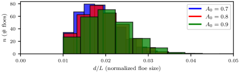
Figure 2: Floe size distributions for different global sea ice concentrations $A_{0}$ and a total number of ice floes $n=2000$. The floe size $d$ is defined as the square root of the floe area.

We run the DEM simulations for $2\times 10^{4}$ time steps, each of $5\,$\mathrm{s}$$ (the total running time is approximately equal to 27.8 hours). In general, we find that the velocity, stress, and sea ice concentration, averaged over the last 25% of the time steps, remain relatively unchanged when a longer computation is performed, and hence we consider that a steady state has been reached. This temporal averaging is performed over data which, at each time step, has been averaged spatially as described in appendix A.2. For these simulations, the material parameters which determine the effects of the ocean drag and the collisions among floes are presented in table 1. Collisional forces and the resultant stresses, which determine the fields $\boldsymbol{\sigma}$ and $p$, are computed as explained in appendix A.1.

In figure 4 we plot the values of the friction $\mu=|\sigma_{xy}|/p$ and local concentration $A$ against $I$ for different global concentrations $A_{0}$ between $0.7$ and $0.95$ and different maximum ocean velocities $u_{o,max}$ between $0.1$ and $1\,$\mathrm{m}\mathrm{/}\mathrm{s}$$. The mean ocean velocities in the ocean patch are therefore between $0.05$ and 0.5 m/s, values that are consistent with real observations (Stewart et al.,, 2019). In all of these computations, we set the ice thickness to $H=2\,$\mathrm{m}$$. We find an increase in the friction $\mu$ and a decrease in the local concentration $A$ as $I$ increases. The decrease in the local concentration of sea ice $A$ with an increase in $I$ is due to dilatancy. Figure 3 presents an example of how dilatancy emerges in the DEM computations: given a random initial distribution of ice floes, when a steady state is reached the concentration $A$ decreases in the areas where the largest shearing occurs ($y=1/4$ and $y=3/4$), and increases elsewhere. Since the global sea ice concentration $A_{0}$ is constant, in this context dilatancy represents a reorganization of the local concentration profile $A(y)$.

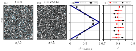
Figure 3: Emergence of dilatancy in the DEM. Here, $A_{0}=0.8$ and $u_{o}=1\,$\mathrm{m}$/$\mathrm{s}$$. Ten runs to steady state are performed from randomized initial conditions, with (a) and (b) being examples of initial and final states, respectively. (c) ocean and sea ice velocities, (d) initial (red) and final (black) mean local sea ice concentration with the standard deviation (bars). Clearly, $A$ decreases in the areas of maximum shear strain, compare (c) and (d).

The trends found in the data in figure 4 are well fitted with the following family of functions:

$$\mu(I)=\mu_{0}+\mu_{1}I\quad\text{and}\quad\Phi(I)=1-\phi_{0}I^{\alpha}.$$ (3.1)

A linear behaviour is also found for $\mu$ in Da Cruz et al., (2005). The four parameters $(\mu_{0},\mu_{1},\phi_{0},\alpha)$ are calculated by minimizing the least-squares misfit problem between the points in figure 4 and the functions in (3.1). The resulting values are shown in table 2. For the remainder of the document, any numerical solution of the one dimensional system (2.15) is solved by setting the parameters in functions (3.1) to the values given in table 2.

$\mu_{0}$	$\mu_{1}$	$\phi_{0}$	$\alpha$
0.26	4.93	0.53	0.24

Table 2: Parameters for the functions $\mu(I)$ and $\Phi(I)$ in (3.1) obtained by minimizing the least-squares misfit with the data plotted in figure 4. These are the numerical values used for computing solutions to the continuous model (2.15) throughout this paper.

Departure from the fitting curves are most visible when the ocean velocities and sea ice concentrations are low, see the case where $u_{o,max}=0.1\,$\mathrm{m}$/$\mathrm{s}$$ and $A_{0}=0.7$. Unsurprisingly, in section 5 below, we also find the greatest misfit between the DEM and the continuous model precisely in this setting, when $u_{o,max}=0.1\,$\mathrm{m}$/$\mathrm{s}$$ and $A_{0}=0.7$, see panel (m) in figure 9 below. In particular, in this setting, the fundamental balance between shear stress and ocean drag in the DEM is found to no longer hold, see section 5.

The constitutive equation in 2D resulting from functions (3.1) is the sum of a plastic and a viscous term:

$$\boldsymbol{\tau}=\underbrace{\mu_{0}p\frac{\boldsymbol{\mathrm{S}}}{\|\boldsymbol{\mathrm{S}}\|}}_{\text{plastic}}+\underbrace{\mu_{1}\overline{d}^{2}\sqrt{\rho_{i}Hp}\,\boldsymbol{\mathrm{S}}}_{\text{viscous}}.$$ (3.2)

A consequence of this linear behavior is that $\mu$ is approximately constant for small values of $I$, and this is precisely what we see for $I<10^{-2}$ in figure 4. For $I\ll 1$, we have that $\mu(I)\approx\mu_{0}$, and therefore it is the plastic term that dominates the rheology. This is essentially the quasi-static regime, where collisions are negligible. This plastic term follows from a Mohr-Coulomb yield criterion with an internal angle of friction $\tan^{-1}(\mu_{0})$; examples of the Mohr-Coulomb yield criterion used for sea ice modeling can be found in Ip et al., (1991), Gutfraind and Savage, (1997) and Ringeisen et al., (2019). The viscous term, which becomes increasingly important as the inertial number $I$ increases, can be associated with the collisional component of the rheology. A viscous rheology is derived in Shen et al., (1987) for modeling the rheological effects of collisions in sea ice, which, as we explain in section 6, is very similar to the viscous component in (3.2).

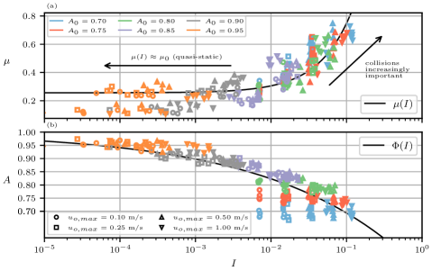
Figure 4: (a) friction $\mu=|\sigma_{xy}|/p$ and (b) concentration $A$ against $I$. Ten friction and concentration values are extracted from each DEM run by averaging along the grid cells plotted in figure 15. The black lines correspond to the functions (3.1) fitted to the data by minimizing the least-squares misfit.

4 Analysis of the inferred continuous model

This section focuses on the one dimensional system of equations presented in section 2.2, with the functions $\mu$ and $\Phi$ taking the form (3.1). In order to understand the relative importance of the different parameters involved in this system of equations, we first rewrite it in a non-dimensional manner. Then, we study the properties of solutions to the momentum equation (2.15b) and the role of plasticity in these solutions. Finally, we consider the complete system of equations, which includes the mass conservation constraint (2.16), and we demonstrate that, under certain conditions, this system has a unique solution. For simplicity, the solutions presented throughout this section result from driving the ice floes with the ocean velocity profile (2.17), although the analysis can be extended to more general ocean velocity profiles by following the same steps.

For the non-dimensionalization, we set the characteristic magnitudes

$$[y]=L,\quad[H]=H,\quad[u]=u_{o,max},\quad\text{and}\quad[\sigma]=\rho_{i}[u]^{2}[H]$$ (4.1)

for the length, thickness, velocity, and stress, respectively. We scale the velocities $u$ and $u_{o}$ with $[u]$, the spatial variables $y$ and $\overline{d}$ with $[y]$, the thickness $H$ with $[H]$, and $\sigma_{xy}$ and $p$ with $[\sigma]$.

From this point onward, all variables considered are non-dimensional unless the contrary is made explicitly clear or units are specified. Keeping the same notation as used for dimensional variables, the following normalized system of equations is derived for $u$, $I$, and $A$, and for the constant $p>0$:

$$-\epsilon\frac{\mathrm{d}}{\mathrm{d}y}\left(\mu_{0}p\frac{\mathrm{d}u/\mathrm{d}y}{|\mathrm{d}u/\mathrm{d}y|}+\mu_{1}\sqrt{p\frac{A_{0}}{n}}\frac{\mathrm{d}u}{\mathrm{d}y}\right)=\beta_{o}|u_{o}-u|(u_{o}-u),$$ (4.2a)

$$I=\sqrt{\frac{A_{0}}{pn}}\left|\mathrm{d}u/\mathrm{d}y\right|.$$ (4.2b)

$$A=1-\phi_{0}I^{\alpha},$$ (4.2c)

$$\int_{0}^{1}A\,\mathrm{d}y=A_{0}.$$ (4.2d)

Here, $\epsilon=H/L$ and $\beta_{o}=\rho_{o}/\rho_{i}C_{o}$; the non-dimensional average floe size $\overline{d}$ is set to $\sqrt{A_{0}/n}$. The system (4.2) is closed by enforcing periodic boundary conditions for $u$, $I$, and $A$. Following our findings in table 2, we assume that the parameters $\mu_{0}$, $\phi_{0}$, and $\alpha$ are strictly greater than zero. We also assume $\mu_{1}>0$ in all but section 4.1.2, where we study the case when $\mu_{1}=0$ with the intention of understanding the plastic component of the momentum equation (4.2a).

All numerical results computed in this section take (2.17) as the ocean velocity, which is written as

$$u_{o}(y)=1-|1-2y|$$ (4.3)

for $y\in(0,1)$ when non-dimensionalized.

4.1 The momentum equation

In order to understand the system of equations (4.2), we first focus on the momentum equation (4.2a). When considering the entire system (4.2), the pressure $p\in\mathbb{R}$ is one of the unknowns. However, it is useful to first assume it to be known, in which case we can solve the momentum equation (4.2a) for $u$ and study the effect of $p$ on $u$. Here, we show that (4.2a) can be understood as a minimization problem. This reformulation of the momentum equation allows us to establish the existence and uniqueness of solutions. Moreover, the optimality conditions for the minimization problem result in a different formulation of the plasticity component of the rheology which avoids the singularity, present in (4.2a), at $\mathrm{d}u/\mathrm{d}y=0$. With this reformulation of the plastic term, we are able to find analytical solutions to the purely plastic problem which arises when $I\ll 1$, near the quasi-static regime.

4.1.1 Reformulation of (4.2a) as a minimization problem

Given a pressure $p>0$, solutions $u$ to (4.2a) minimize the following functional,

$$\mathcal{J}(u):=\epsilon\mu_{0}p\int_{0}^{1}\left|\frac{\mathrm{d}u}{\mathrm{d}y}\right|\,\mathrm{d}y+\frac{\epsilon\mu_{1}}{2}\sqrt{p\frac{A_{0}}{n}}\int_{0}^{1}\left|\frac{\mathrm{d}u}{\mathrm{d}y}\right|^{2}\,\mathrm{d}y+\frac{\beta_{o}}{3}\int_{0}^{1}|u_{o}-u|^{3}\,\mathrm{d}y$$ (4.4)

over the space of velocity profiles

$$V:=\left\{v\in H^{1}((0,1)):\text{$v$ is a periodic function}\right\}.$$ (4.5)

In the definition of $V$, the space $H^{1}((0,1))$ denotes the Sobolev space of weakly differentiable and periodic functions on the unit interval (Adams and Fournier,, 2003). As explained in appendix B, the functional $\mathcal{J}$ is strictly convex and coercive over $V$ and therefore admits a unique minimizer. In this sense, one can state that the momentum equation (4.2a) also has a unique solution.

To derive (4.2a) for the minimizer $u$ of $\mathcal{J}$, we first note that, if $u$ minimizes $\mathcal{J}$, then

$$\frac{1}{t}\left(\mathcal{J}(u+t(v-u))-\mathcal{J}(u)\right)\geq 0\quad\forall v\in V,\,\forall t\in(0,1).$$ (4.6)

The three terms in the right hand size of (4.4) are convex, with the two last ones differentiable over all $V$. By exploiting the convexity of the first term (the $L^{1}$ norm) and the differentiability of the other two terms, we find that

$$\begin{split}\epsilon\mu_{0}p\left(\left|\frac{\mathrm{d}v}{\mathrm{d}y}\right|-\left|\frac{\mathrm{d}u}{\mathrm{d}y}\right|\right)+\epsilon\mu_{1}\sqrt{p\frac{A_{0}}{n}}\int_{0}^{1}\frac{\mathrm{d}u}{\mathrm{d}y}\frac{\mathrm{d}(v-u)}{\mathrm{d}y}\,\mathrm{d}x\\ -\beta_{o}\int_{0}^{1}|u_{o}-u|(u_{o}-u)(v-u)\,\mathrm{d}x\geq 0\quad\forall v\in V.\end{split}$$ (4.7)

A variational statement as in (4.7) is known as a variational inequality. Under the assumption that the solution $u$ is not only in $V$ but is twice continuously differentiable, we may deduce that

$$-\epsilon\frac{\mathrm{d}}{\mathrm{d}y}\left(\sigma_{xy}^{P}+\mu_{1}\sqrt{p\frac{A_{0}}{n}}\frac{\mathrm{d}u}{\mathrm{d}y}\right)=\beta_{o}|u_{o}-u|(u_{o}-u),$$ (4.8a)

$$|\sigma_{xy}^{P}|\leq\mu_{0}p,$$ (4.8b)

$$\sigma_{xy}^{P}\left|\frac{\mathrm{d}u}{\mathrm{d}y}\right|=\mu_{0}p\frac{\mathrm{d}u}{\mathrm{d}y}.$$ (4.8c)

A similar derivation to that of (4.8) from (4.7) can be found in (Glowinski et al.,, 1981, section 1.3). In (4.8), we have introduced $\sigma_{xy}^{P}$, the purely plastic component of the shear stress. Introducing this new variable allows us to reformulate (4.2a) such that the singularity at $\mathrm{d}u/\mathrm{d}y=0$ is removed. Indeed, if $\mathrm{d}u/\mathrm{d}y\neq 0$, it is clear that (4.8) is equivalent to (4.2a). In this case, we have that $|\sigma_{xy}^{P}|=\mu_{0}p$ and we say that the material has reached its plastic yield strength $\mu_{0}p$. Conversely, when $\mathrm{d}u/\mathrm{d}y=0$, (4.8a) remains well defined, unlike (4.2a). We remark that $\mathrm{d}u/\mathrm{d}y=0$ must follow from (4.8c) whenever $|\sigma_{xy}^{P}|<\mu_{0}p$ (the material has not reached its plastic yield strength). Below, in section 4.1.2, we provide further insight into the plastic component of the shear stress by computing purely plastic solutions to the momentum equation analytically.

The first order optimality condition for the minimization of $\mathcal{J}$ are a variational inequality (rather than a variational equality) because the first term to the right hand side of (4.4) (the $L^{1}$ norm) is non differentiable when $\mathrm{d}u/\mathrm{d}y=0$. We can make $\mathcal{J}$ differentiable by regularizing it as follows:

$$\mathcal{J}_{\Delta}(u):=\epsilon\mu_{0}p\int_{0}^{1}\sqrt{\left|\frac{\mathrm{d}u}{\mathrm{d}y}\right|^{2}+\Delta^{2}}\,\mathrm{d}y+\frac{\epsilon\mu_{1}}{2}\sqrt{p\frac{A_{0}}{n}}\int_{0}^{1}\left|\frac{\mathrm{d}u}{\mathrm{d}y}\right|^{2}\,\mathrm{d}y+\frac{\beta_{o}}{3}\int_{0}^{1}|u_{o}-u|^{3}\,\mathrm{d}y,$$ (4.9)

where $\Delta>0$ is a small parameter. The first order optimality conditions for the minimization of $\mathcal{J}_{\Delta}$ over $V$ corresponds with the following equation:

$$-\epsilon\frac{\mathrm{d}}{\mathrm{d}y}\left(\mu_{0}p\frac{\mathrm{d}u/\mathrm{d}y}{\sqrt{|\mathrm{d}u/\mathrm{d}y|^{2}+\Delta^{2}}}+\mu_{1}\sqrt{p\frac{A_{0}}{n}}\frac{\mathrm{d}u}{\mathrm{d}y}\right)=\beta_{o}|u_{o}-u|(u_{o}-u).$$ (4.10)

Although the system (4.8) can be solved numerically by e.g. introducing a Lagrange multiplier (Glowinski et al.,, 1981), it is easier to solve equation (4.10). This is the strategy we take for solving the momentum equation and, as we explain below in section 4.2.1, the complete system (4.2). To do so, we use the finite element method (FEM) implemented in Firedrake (Ham et al.,, 2023). In particular, we approximate the velocity profile $u$ with continuous piece-wise linear functions. In figure 5, we plot solutions to (4.10) for two different values of $p$ and a range of $\Delta>0$. Convergence of the velocity profiles as $\Delta\to 0$ is clearly visible in these figures; in fact, for $\Delta\leq 10^{-2}$, the solutions become indistinguishable. We remark that, if we remove the viscous component of the rheology in the regularized equation (4.10), we essentially arrive at Hibler’s model in one dimension, given below by (6.1a).

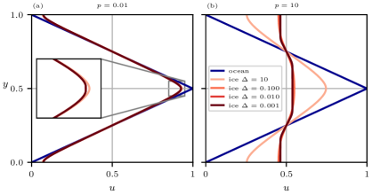
Figure 5: Solutions $u$ to the momentum equation (4.10) for different values of the ice pressure $p$ and the numerical regularization parameter $\Delta$. We set $u_{o}$ equal to (2.17), normalized with $[u]=u_{o,max}$, and $\epsilon=2\times 10^{5}$, $A_{0}=0.8$ and $n=2000$. We observe convergence to a solution as $\Delta\to 0$ and, for small $p$, $u\to u_{o}$ in (a) and, for large $p$, $u\to 0.5$ in (b), as expected from the theory.

The pressure or ice strength $p$ is a fundamental variable in the continuous model; understanding its effect on $u$ is fundamental for making sense of our sea ice model. Figure 5 suggests that, for small $p$, the velocity profile $u$ approaches the ocean’s $u_{o}$ and, for large $p$, $u$ flattens and comes close to a constant-valued velocity profile. We can deduce this behavior from the functional $\mathcal{J}$. For small values of $p$,

$$\lim_{p\to 0}\mathcal{J}(u)=\frac{\beta_{o}}{3}\int_{0}^{1}|u_{o}-u|^{3}\,\mathrm{d}y,$$ (4.11)

and therefore, since $u$ minimizes $\mathcal{J}$, it must follow that $u\to u_{o}$. On the other hand, for large values of $p$, we see that

$$\mathcal{J}(u)\approx\epsilon\mu_{0}p\int_{0}^{1}\left|\frac{\mathrm{d}u}{\mathrm{d}y}\right|\,\mathrm{d}y\quad\text{as $p\to\infty$}$$ (4.12)

and, in principle, any constant velocity profile $u_{c}\in\mathbb{R}$ minimizes (4.12). However, this constant velocity field is constrained by the total force balance of the system. That is, due to the periodic boundary conditions, if we integrate (4.8a) along $(0,1)$, we must have that

$$\beta_{o}\int_{0}^{1}|u_{o}-u|(u_{o}-u)\,\mathrm{d}y=0.$$ (4.13)

Therefore, the constant value to which $u$ tends as $p\to\infty$ will be a solution to (4.13) with $u=u_{c}\in\mathbb{R}$. Below, in section 4.1.2, we show that a critical pressure $p_{c}$ can be found such that $u$ is constant whenever $p>p_{c}$ and $I\ll 1$.

4.1.2 Purely plastic solutions to the momentum equation

In figure 4 we can see that $\mu(I)$ roughly becomes constant for small inertial numbers $I\ll 1$, such that $\mu(I)\approx\mu_{0}$ and the flow rheology is plastic. This regime is closely related to the quasi-static regime for granular media, with the material behaving like a purely plastic flow characterized by a critical state at which plastic deformation occurs (Wood,, 1990).

The momentum equation to the purely plastic problem where $\mu(I)=\mu_{0}$ is given by

$$\epsilon\frac{\mathrm{d}\sigma_{xy}^{P}}{\mathrm{d}y}=-\beta_{o}|u_{o}-u|(u_{o}-u).$$ (4.14)

Equation (4.14) must be complemented with (4.8b) and (4.8c). Here, we present a method for calculating solutions to (4.20). Additionally, we find a critical pressure $p_{c}$ such that, for $p>p_{c}$, the velocity profiles $u$ that solve (4.14) remain constant and no shear strain occurs in the sea ice. In section 5 below, we show that this critical pressure approximates the pressure computed from the DEM when the global sea ice concentration is high. When following the derivation of purely plastic solutions, it is helpful to look at their plots in figure 6 below.

Conditions (4.8b) and (4.8c) for the plastic stress tensor indicate that there exist two distinct regions of the flow field: a region where the sea ice has yielded and $|\sigma_{xy}^{P}|=p\mu_{0}$, and another region where the ice has not yielded and $|\sigma_{xy}^{P}|\leq p\mu_{0}$ and $\mathrm{d}u/\mathrm{d}y=0$. By working with this distinction, we can find a purely plastic solution to (4.14). Due to the symmetry of the problem, we assume that $\sigma_{xy}^{P}=0$ at $y=0$, $1/2$, and $1$. Then, integrating (4.14) along the interval $(0,y)$ for some $y\in(0,1)$, we find that

$$\sigma_{xy}^{P}(y)=-\frac{\beta_{o}}{\epsilon}\int_{0}^{y}|u_{o}-u|(u_{o}-u)\,\mathrm{d}y.$$ (4.15)

Since $\sigma_{xy}^{P}(0)=0$, we must necessarily have an interval $(0,y_{1})$ where the ice has not yielded and the velocity equals a constant $u_{1}$. In the context of the ocean velocity profile (4.3), it makes sense to assume that $u_{1}>0$, and therefore $u_{1}\geq u_{o}$ near $y=0$, so that

$$\sigma_{xy}^{P}(y)=\frac{\beta_{o}}{6\epsilon}\left((2y-u_{1})^{3}+u_{1}\right).$$ (4.16)

Since the material has not yielded for $y\in(0,y_{1})$, we have that $|\sigma_{xy}^{P}(y)|<\mu_{0}p$. Equation (4.16) tells us that $\sigma_{xy}^{P}(y)$ increases with $y$ over this interval; this means that

$$\lim_{y\to y_{1};y<y_{1}}\sigma_{xy}^{P}(y)=\mu_{0}p,$$ (4.17)

and we find that

$$u_{1}=\left(\frac{6\epsilon\mu_{0}p}{\beta_{0}}\right)^{1/3}.$$ (4.18)

Clearly, an upper bound is needed for $u_{1}$ in (4.18), because it grows indefinitely with $p$, yet it is senseless for the ice to circulate at speeds greater than the maximum ocean velocity when a steady state has been reached. We can make sense of this paradox by firstly assuming the existence of an interval $(y_{1},y_{2})$, where $y_{1}<y_{2}<1/2$, in which the sea ice has yielded and $\sigma_{xy}^{P}=\mu_{0}p$. In this interval we must have that $u=u_{o}$ because $\sigma_{xy}^{P}$ is constant and therefore the ocean drag is zero. This means that $y_{1}=u_{1}/2$. Moreover, repeating the same argument as that used for deriving (4.18), we assume that $u=u_{2}$ for some constant $u_{2}<1$ on $(y_{2},1/2)$ and find that $u_{2}=1-u_{1}$ and $y_{2}=u_{2}/2$. Now, the assumption that $y_{1}<y_{2}<1/2$ will only hold for values of $p$ for which $u_{1}\leq u_{2}$; that is, $u_{1}\leq 1/2$, and this upper bound on $u_{1}$ defines a critical pressure $p_{c}$ given by

$$p_{c}=\frac{\beta_{o}}{48\epsilon\mu_{0}}.$$ (4.19)

For $p\geq p_{c}$, the integral force balance along the domain must hold, see (4.13); as a result, $u_{1}$ can be at most equal to $1/2$. Putting these results together, we may write the analytical solution to (4.14) as

$$u(y)=\left\{\begin{array}[]{cl}u_{1}&\text{ $0<y<\frac{u_{1}}{2}$},\\ u_{o}(y)&\text{$y_{1}<y<\frac{1}{2}-y_{1}$},\\ 1-u_{1}&\text{$\frac{1}{2}-y_{1}<y<\frac{1}{2}$},\end{array}\right. \text{if $p<p_{c}$},$$ (4.20d)

$$u(y)=\frac{1}{2} \text{if $p\geq p_{c}$}.$$ (4.20e)

for $y\in[0,1]$. We test the validity of (4.20) by showing that it is indistinct from its numerical counterpart in figure 6. We compute this numerical solution by regularizing the shear stress $\sigma_{xy}^{P}$ as in (4.10) and setting $\Delta=10^{-3}$.

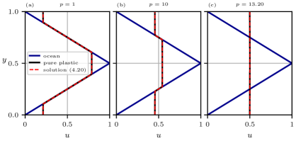
Figure 6: Solutions $u$ to the purely plastic momentum equation (4.14). We use the same parameter values as those used for figure 5 and $\Delta=10^{-2}$. The numerical solutions (black) to the purely plastic problem are indistinguishable from the analytical solution given by (4.20) (red, dotted). As the ice pressure $p$ increases, the velocity profiles flattens at the critical pressure $p_{c}$ given by (4.19) and $p_{c}\approx 13.2$ in this case.

4.2 Solutions to the continuous model

In section 4.1, we have seen that, given a value for the pressure $p$, we can solve the momentum equation and find a velocity profile $u$ for the sea ice. We also prove that solutions to the momentum equation must exist and be unique. However, in general, the pressure $p$ is one of the unknowns in the system of equations (4.2), together with the sea ice concentration $A$ and the inertial number $I$. Here, we first present a numerical method for solving (4.2) and show that solutions to this system always exist and, under some circumstance, are unique.

4.2.1 A numerical method for the complete model (4.2)

In order to solve the system (4.2), we follow the approach discussed in section 4.1.1 for solving the momentum equation. There, the regularized equation (4.10) is solved numerically with the FEM. When solving the complete system (4.2), we find that also regularizing the inertial number $I$ improves the convergence properties of our numerical solver substantially. Therefore, we solve for

$$I_{\Delta}:=\sqrt{\frac{A_{0}}{pn}\left(\left|\frac{\mathrm{d}u}{\mathrm{d}y}\right|^{2}+\Delta^{2}\right)}\quad\text{and}\quad A=1-\phi_{0}I_{\Delta}^{\alpha}$$ (4.21)

instead of (4.2b) and (4.2c). Then, we use the FEM to solve the system of equations given by the regularized momentum equation (4.10), (4.21), and the constraint for global concentration (4.2d). We approximate $u$ with continuous piece-wise linear functions and $I_{\Delta}$ and $A$ with piece-wise constant functions. Our solver is implemented in Firedrake (Ham et al.,, 2023) in such a way that the complete nonlinear system is solved with Newton’s method. For small values of $\Delta$, Newton’s method tends to fail unless a very good initial guess for the solution $(u,I_{\Delta},A,p)$ is given. For this reason, we find that solving for a sequence of decreasing values of $\Delta$, using the solution for the previous $\Delta$ as the initial guess for the next $\Delta$, yields a robust solution method.

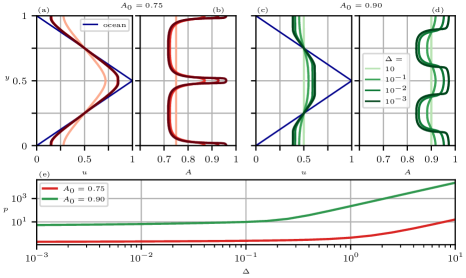
Figure 7: Solutions $u$ and $A$ to the continuous model (4.2) with $A_{0}=0.75$ ((a),(b)) and $A_{0}=0.9$ ((c),(d)), regularized with a parameter $\Delta$ as explained in section 4.2.1. In (e) we plot the variation of the pressure $p$ with $\Delta$. We use the same parameter values as those used for figure 5.

We test the sensitivity of solutions $(u,I_{\Delta},A,p)$ to changes in $\Delta$ by solving the system for values of $\Delta$ between $10^{-3}$ and $10$ and for $A_{0}=0.75$ and $A_{0}=0.9$. The numerical results, which are plotted in figure 7, indicate that the solutions become more sensitive to $\Delta$ as $A_{0}$ increases; this is natural, since $I$ decreases with $A_{0}$ and the plasticity term becomes more important. It is also clear from these plots that, although the velocity profiles $u$ come very close to convergence for the smallest values of $\Delta$, the local concentration profiles still experience visible changes around the symmetry points $y=0$, $0.5$, and 1. In these points the shear strain drops to 0 and, by the definition of $I$, we expect $A=1$ there. However, as we argue below in section 5, when comparing the continuous model and the DEM, we consider such drastic changes in the local concentration to be artificial. This argument motivates the use of $\Delta$ not just as a numerical parameter that helps us solve the system numerically, but as a parameter that improves the model and may have a physical significance.

4.2.2 Existence and uniqueness of solutions

We conclude the analysis of the continuous model by showing that at least one solution to (2.15) must exist and, whenever $u_{o}$ is given by (2.17), is unique. To do so, we first reformulate (2.15) solely in terms of $u$ and $p$ by eliminating $A$ and $I$ as follows. Substituting (4.2c) into (4.2d) yields

$$\int_{0}^{1}I^{\alpha}\,\mathrm{d}y=\frac{1-A_{0}}{\phi_{0}}.$$ (4.22)

Then, by substituting the definition of $I$, equation (4.2b), into the integrand in the expression above, we arrive at

$$\int_{0}^{1}\left|\frac{\mathrm{d}u}{\mathrm{d}y}\right|^{\alpha}\mathrm{d}y=\frac{1-A_{0}}{\phi_{0}}\left(p\frac{n}{A_{0}}\right)^{\frac{\alpha}{2}}.$$ (4.23)

Therefore, the system of equations (4.2) is equivalent to solving the momentum equation (4.2a) together with the constraint (4.23) for $u$ and $p$. We can interpret this problem as the minimization of the functional (4.4) over a set of velocity profiles subject to the constraint (4.23). Next, we define $\mathcal{F}:\mathbb{R}_{+}\to\mathbb{R}_{+}$ by

$$\mathcal{F}(p):=\int_{0}^{1}\left|\frac{\mathrm{d}u}{\mathrm{d}y}\right|^{\alpha}\mathrm{d}y,$$ (4.24)

with $u$ denoting the solution to (4.2a) with the pressure set to $p$; this operator is well-defined because, given a pressure $p>0$, a unique velocity profile $u$ solves the momentum equation (4.2a). We also define $\mathcal{C}:\mathbb{R}_{+}\to\mathbb{R}_{+}$, given by the left hand side of (4.23), that is,

$$\mathcal{C}(p):=\frac{1-A_{0}}{\phi_{0}}\left(p\frac{n}{A_{0}}\right)^{\frac{\alpha}{2}}.$$ (4.25)

It is then clear that a pressure $p$ is part of the solution to the system of equations (4.2) if and only if

$$\mathcal{C}(p)=\mathcal{F}(p).$$ (4.26)

In section 4.1 we show that the velocity profile $u$ has two distinct limit behaviors. We find that $u$ approaches $u_{o}$ as $p\to 0$ and that $\mathrm{d}u/\mathrm{d}y$ tends to $0$ as $p\to\infty$. This means that

$$\lim_{p\to 0}\mathcal{F}(p)=\int_{0}^{1}\left|\frac{\mathrm{d}u_{o}}{\mathrm{d}y}\right|^{\alpha}\mathrm{d}y\quad\text{and}\quad\lim_{p\to\infty}\mathcal{F}(p)=0.$$ (4.27)

On the other hand, the function $\mathcal{C}$ is strictly increasing, with $\mathcal{C}(0)=0$. Therefore, whenever $\int_{0}^{1}\left|\mathrm{d}u_{o}/\mathrm{d}y\right|^{\alpha}\mathrm{d}y>0$ (that is, $u_{o}$ is not a flat velocity profile) and $\mathcal{F}$ is a continuous function, we must have at least one solution $p$ to (4.26). Moreover, if $\mathcal{F}$ is a decreasing function, this pressure must be unique.

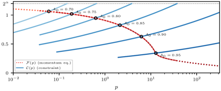
Figure 8: Functions $\mathcal{F}(p)$ and $\mathcal{C}(p)$, defined in (4.24) and (4.25), respectively, for different values of $A_{0}$. The lighter tones of blue and red are associated with lower values of $A_{0}$, although $\mathcal{F}$ hardly changes with $A_{0}$. A pressure $p$ solves (2.15) whenever $\mathcal{C}(p)=\mathcal{F}(p)$ (circles). To generate these curves numerically, the same problem setting as that of figure 5 is used.

In Figure 8, we plot the functions $\mathcal{C}$ and $\mathcal{F}$ for several values of $A_{0}$ and an ocean velocity profile given by (4.3). In this case, we have that

$$\int_{0}^{1}\left|\frac{\mathrm{d}u_{o}}{\mathrm{d}y}\right|^{\alpha}\mathrm{d}y=2^{\alpha}$$ (4.28)

and the function $\mathcal{F}$ appears to be strictly decreasing. This is expected, because an increase in pressure is accompanied by a flattening of the sea ice velocity profile. This means that there is a unique $p$ for which (4.26) holds; since there is only one velocity profile $u$ that solves the momentum equation (4.2a), it follows that the solution to the continuous model (4.2) must be unique.

5 Comparison of the DEM with the continuous model

The continuous model (4.2) is designed with the objective of capturing the averaged behavior of the sea ice simulations carried out with the DEM. Here, we verify that, in the one dimensional setting of the steady ocean periodic problem, the continuous model is indeed capable of replicating most of the results of the DEM. Throughout this section, we use the parameters in tables 1 and 2 when solving the continuous model. The continuous system is solved as explained in section 4.2.1 with $\Delta=10^{-3}$ and a uniform mesh of 300 cells.

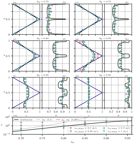
Figure 9: Solutions to the non-dimensional continuous system (4.2) (black lines) compared with results from the DEM (markers), with the ocean velocity in blue. For each pair of panels in the first three rows, we fix the global sea ice concentration $A_{0}$, vary the maximum ocean velocity $u_{o,max}$ for the DEM, and plot the velocities in the panels to the left ((a), (c), (e), (g), (i), and (k)) and the local concentration to the right ((b), (d), (f), (h), (j), and (l)). In panel (m), we plot the pressure $p$ in terms of $A_{0}$. Due to the normalization in terms of $[u]=u_{o,max}$, the solutions to the continuous model are indifferent to a change in $u_{o,max}$.

5.1 Variation in global concentration $A_{0}$ and ocean speed $u_{o,max}$

We first evaluate the continuous model’s accuracy in replicating the DEM results used for fitting the functions $\mu(I)$ and $\Phi(I)$ in section 3. These results are computed for the ocean velocity profile (2.17) and an ice thickness of $H=2\,$\mathrm{m}$$. We consider six global sea ice concentrations $A_{0}$ between $0.7$ and $0.95$ and four ocean velocities $u_{o,max}$ between $0.1$ and $1\,$\mathrm{m}$/$\mathrm{s}$$. For each of these cases, we run the DEM until a steady state is reached and then we extract 10 values of the sea ice velocity and concentration along the $y$-direction, as explained in section 3, and one value for the pressure $p$, averaged over the whole square patch of ocean.

Figure 9 displays the velocity and sea ice concentration profiles $u$ and $A$ and the pressure $p$ for both the continuous model and the DEM. The velocity profile $u$ and the pressure $p$ are normalized as explained in section 4 using $[u]=u_{o,max}$. A consequence of this normalization is that the non-dimensional solutions $u$, $A$, and $p$ to the continuous model (4.2) are indifferent to the value of $u_{o,max}$. For most of the DEM results, this is also the case. For each value of $A_{0}$, almost all of the normalized velocity profiles (panels (a), (c), (e), (g), (i), and (k)) and pressure points (panel (m)) appear to collapse onto a single curve or point, which is well approximated by the continuous model.

Departures from the other normalized DEM results are most visible for slow ocean currents and low concentrations. This becomes particularly clear when looking at the pressure in panel (m) when $u_{o,max}=0.1\,$\mathrm{m}$/$\mathrm{s}$$ and $A_{0}\leq 0.8$, where the pressure values from the DEM (circles) depart substantially from the prediction of the continuous model (black solid line). These mismatches signal the continuous model’s limitations to capture the DEM results for the range of regimes considered. When fitting the dilatancy function $\Phi(I)$, the largest misfit is also found for points of slow ocean currents and low concentration ($u_{o,max}=0.1\,$\mathrm{m}$/$\mathrm{s}$$ and $A_{0}\leq 0.75$), see panel (b) in figure 4. If the DEM results are to approximate a continuous model as in (4.2), we expect the equality

$$\sigma_{xy}(y)=-\int_{0}^{y}t_{ox}\,\mathrm{d}y,$$ (5.1)

to hold approximately for the DEM results, with $t_{ox}$ denoting the horizontal component of the ocean drag. If we denote by $\sigma_{xy,i}$ and $t_{ox,i}$ the values extracted from the DEM at the grid cell of width $\Delta y$ located at $y_{i}$ (see appendix A.2 for an overview of how these quantities are obtained), a discrete balance analogous to (5.1) is

$$\sigma_{xy,i}=-\Delta y\sum_{j=1}^{i}t_{ox,j}.$$ (5.2)

We remark that the term $t_{ox,j}$ results from averaging the ocean drag on each ice floe, as opposed to introducing the averaged sea ice velocity into (2.5). We also note that (5.2) ignores any choice of rheology and should hold independently of our choice of functions $\mu(I)$ and $\Phi(I)$. A surprising result we find when investigating the DEM data is that the terms to the left and right hand side of the equality in (5.2) differ in orders of magnitude whenever the sea ice concentration is low and the ocean currents are slow, see panel (a) of figure 10. Conversely, for faster ocean currents and denser concentrations, these terms become approximately equal (see panels (c)-(f) in figure 10). Inertial effects are found to be negligible in all of the cases we consider; moreover, since DEM quantities are averaged along the whole length of the domain in the $x$-direction, the term corresponding to $\partial\sigma_{xx}/\partial x$, which should be considered in a two-dimensional setting, becomes zero. Therefore, this finding raises the questions of whether a fundamentally different continuous model should be used for low sea ice concentrations and slow ocean currents or if a continuous model is valid at all.

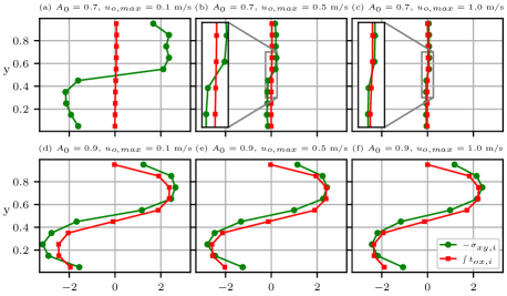
Figure 10: Shear stress $\sigma_{xy,i}$ and integrated ocean drag $\int t_{ox,i}:=\Delta y\sum_{j=1}^{i}t_{ox,j}$ extracted from the DEM for $A_{0}=0.7$ and $0.9$ and $u_{o,max}=0.1$, 0.5 and $1\,$\mathrm{m}\mathrm{/}\mathrm{s}$$.

The DEM’s local concentration $A$ is accurately captured by the continuous model for low sea ice concentrations (panels (b), (d), (f), and (h) in figure 9). For $A_{0}=0.90$ and 0.95 (panels (j) and (l)), the continuous model overestimates the degree of dilatancy, although the general trends are visibly similar, with regions of higher concentration around $y=0$, $1/2$, and $1$, where the strain rates are lowest. Since an increase in $\Delta$ diminishes the local variations in $A$ (see figure 7), this suggests that $\Delta$ could be adjusted to improve the fit with the data. In this case, it would enter the model as a physical parameter whose interpretation should be explored further.

In panel (m) of figure 9, we also test two limit approximations of the pressure which we find in section 4 when $u_{o}$ is given by 4.3. When $p\ll 1$, which occurs for the smaller values of $A_{0}$, we expect $\mathcal{C}(p)\approx 2^{\alpha}$ because $u\approx u_{o}$. This implies that

$$p\approx 4\frac{A_{0}}{n}\left(\frac{\phi_{0}}{1-A_{0}}\right)^{2/\alpha}\quad\text{as $A_{0}\to 0$}.$$ (5.3)

On the other hand, high values of $A_{0}$ result in $I\ll 1$, see figure 4, and therefore $\mu(I)\approx\mu_{0}$, leading to the purely plastic regime studied in section 4.1.2. Panel (k) shows that the velocity profiles are mostly flat in this region, suggesting that the critical pressure $p_{c}$ calculated in (4.19) is a good approximation of the $p$. By plotting (5.3) and $p_{c}$ in panel (m), we find that these are indeed good approximations in their respective limits.

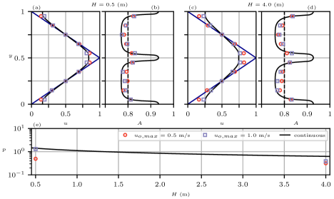
Figure 11: Solutions to the non-dimensional continuous system (4.2) (black lines) compared with results from the DEM (markers). For each pair of panels in the first row, we fix the sea ice thickness $H$ and vary the maximum ocean velocity $u_{o,max}$ (the ocean velocity is plotted in blue in panels (a) and (c)). In panel (e), we plot the pressure $p$ in terms of $H$. Due to the normalization in terms of $[u]=u_{o,max}$, the solutions to the continuum system are indifferent to a change in $u_{o,max}$.

5.2 Variation in ice thickness and number of floes

Next, we test the effectiveness of the continuous model in capturing the DEM results for different ice thicknesses and floe sizes. In figure 11, we plot results for the DEM and the continuous model for steady states with $H=0.5$ and $H=4\,$\mathrm{m}$$, different ocean velocities $u_{o,max}$, and a global sea ice concentration of $A_{0}=0.8$. The ice thickness $H$ enters the continuous model via the parameter $\epsilon=H/L$ in the momentum equation (4.2a). An increase in $H$ is accompanied by an increase in $\epsilon$, which effectively acts as a decrease in the normalized external forcing. We therefore expect an increase in $H$ to result in a decrease in the shear strain and pressure. As observed in panels (a) and (c) of figure 11, this is the case for the velocity profiles of both the continuous model and the DEM; an increase in $H$ is accompanied by a flattening of the normalized velocity profiles. The continuous model is once again accurate in capturing the averaged velocities of the DEM and the general trends in the variation of the sea ice concentration. The pressure resulting from the continuous model and the DEM also decreases as the ice thickness increases, see panel (f); for the pressure, we find a decent fit between the DEM and the continuous model.

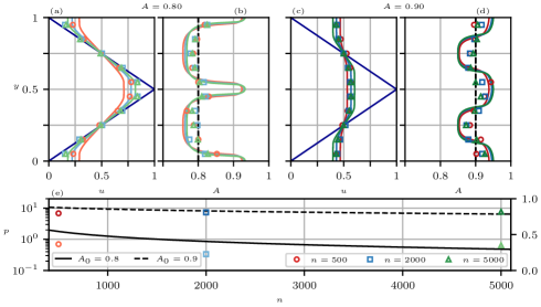
Figure 12: Solutions to the non-dimensional continuous system (4.2) (black lines) compared with results from the DEM (markers). For each pair of panels in the first row, we fix the sea ice thickness $H$ and vary the maximum ocean velocity $u_{o,max}$ (the ocean velocity is plotted in blue in panels (a) and (c)). In panel (e), we plot the pressure $p$ in terms of $n$.

Finally, figure 12 contains a comparison between the DEM and the continuous model for different numbers of floes $n$. In particular, we present results with $n=500$, 2000 and 5000 for $A_{0}=0.8$ and $0.9$ and $u_{o,max}=0.5\,$\mathrm{m}$/$\mathrm{s}$$. An increase in $n$ implies a decrease in the effective viscosity of the model, and we therefore expect a decrease in the ice strength or pressure $p$; in the limit where $n\to\infty$, the rheology becomes purely plastic, this can be seen by taking this limit in (4.2a). In figure 12, one can see that the pressure in continuous model indeed decreases with $n$, but this is not the case with the DEM. In fact, the results of the DEM appear to change little with $n$, especially for $A_{0}=0.9$. Despite this, the results from the DEM do not depart from those of the continuous model excessively.

6 Comparisons with existing models for sea ice

The continuous model studied in this paper shares features with existing models for sea ice. Here, we examine those similarities and also establish differences with our continuous model. Due to its ubiquity in sea ice modeling, we first consider Hibler’s model in section 6.1, before considering other models in section 6.2.

6.1 Hibler’s model

The most widely used model for sea ice is Hibler’s model, which was first presented in Hibler III, (1979) and treats sea ice like a viscoplastic material. Under the one dimensional conditions of the steady square ocean patch and the non-dimensionalization in section 4, Hibler’s model reduces to the following form:

$$-\epsilon\frac{\mathrm{d}}{\mathrm{d}y}\left(\frac{p}{2e}\frac{\mathrm{d}u/\mathrm{d}y}{\sqrt{|\mathrm{d}u/\mathrm{d}y|^{2}+\delta^{2}}}\right)=\beta_{o}|u_{o}-u|(u_{o}-u),$$ (6.1a)

$$p=\frac{P^{\ast}}{\rho_{i}u_{o,max}^{2}}\exp{(-20(1-A))}.$$ (6.1b)

In (6.1), the parameter $P^{\ast}$ is an empirical constant, $\delta$ is a regularization parameter, and $e=2$ represents the eccentricity of the elliptical yield curve from which Hibler’s model is derived. That is, Hibler’s model assumes a plastic rheology based on an elliptical yield curve which is then regularized. Inside the plane of principal stresses, the yield curve is set in such a way that the ice only resists compression, not pure extension. This geometrical configuration is motivated by the observation that, in pack ice, deformation occurs through ridging (compression) and the opening of leads (extension); of these two mechanisms, only ridging requires a non-negligible amount of plastic work (Rothrock,, 1975).

In the steady one dimensional setting, equation (6.1a) can be recovered from the regularized momentum equation (4.10) by setting $\mu_{0}=1/(2e)$ and $\mu_{1}=0$ (pure plasticity). In fact, $1/(2e)=0.25$, which comes very close to the value $\mu_{0}=0.26$ which we infer from the DEM. This means that close to the quasi-static regime, when $I\ll 1$ and $\mu(I)\approx\mu_{0}$, we essentially work with the momentum equation from Hibler’s model. This is a very reasonable coincidence, because Hibler’s model was designed for the central ice pack where the sea ice concentration is very high.

The main departure between our model and Hibler’s is the expression for the pressure (6.1b): as $u_{o,max}$ increases, $p$ decreases in Hibler’s model, unlike our continuous model where $p$ is independent of $u_{o,max}$. This makes it impossible for Hibler’s model to capture the invariance of the non-dimensional sea ice velocity and pressure with $u_{o,max}$ which we find in most of the DEM results in section 5. This is made clear in figure 13, where we show solutions to Hibler’s model and compare them with the DEM for different values of $A_{0}$ and $u_{o,max}$; an increase in $u_{o,max}$ is accompanied by excessively large changes in the velocity profile. We set $P^{\ast}=5\times 10^{4}\,$\mathrm{N}$$\mathrm{m}$^{-1}$ and $\delta=0.1$ n order to get a good fit with the DEM for some values of $u_{o,max}$. We remark that Hibler’s model is designed for ice that fractures and ridges; in this setting, an increase in the ocean drag weakens the ice through this mechanical deformation. Below, in section 7, we state that future extensions of our continuous model should include the effects of fracturing and ridging, available in SubZero. These future investigations should study the validity of (6.1b) when fracturing and ridging are accounted for.

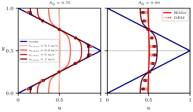
Figure 13: Solutions to Hibler’s model for different global concentrations $A_{0}$ and ocean velocities $u_{o,max}$. We also plot the results from the DEM as a reference. Here, we set $H=2\,$\mathrm{m}$$ and $n=2000$.

The choice of an elliptical yield curve in Hibler’s model is motivated by the simplicity of the resulting rheological formulation, yet other possibilities consistent with the requirement of null resistance to pure extension are available, such as the parabolic lens and the teardrop yield curves (Zhang and Rothrock,, 2005; Ringeisen et al.,, 2023) and the Mohr-Coulomb criterion (Ip et al.,, 1991). In fact, as mentioned at the end of section 3, the purely plastic rheology in the $\mu(I)$ formulation considered here (given by (3.2) with $\mu_{1}=0$), can be written as the Mohr-Coulomb rheology presented in Ip et al., (1991) and Gutfraind and Savage, (1997). This becomes clear if we note that $\|\boldsymbol{\mathrm{S}}\|=\mathrm{D}_{1}-\mathrm{D}_{2}$, where $\mathrm{D}_{1}$ and $\mathrm{D}_{2}$ denote the principal components (eigenvalues) of $\boldsymbol{\mathrm{D}}$, and we compare the plastic component in (3.2) with expression (6) in Gutfraind and Savage, (1997). A significant difference between the two expressions is that in (6) from Gutfraind and Savage, (1997) the viscosity is capped to a maximum value in order to avoid the inevitable blow-up that occurs with a purely plastic rheology; this is another form of regularization. This difference of plastic yield curves between Hibler’s model and the purely plastic version of our model is another point of departure between both models in a two dimensional setting.

6.2 Other models

In section 3, we explain that the viscous component in (3.2) can be interpreted as the rheological effects of collisions, which become increasingly important as $I$ increases. As mentioned in that section, a collisional rheology is derived in Shen et al., (1987) which is also of a linearly viscous nature. In fact, this collisional rheology establishes a viscosity which is linearly proportional to $\overline{d}\sqrt{\rho_{i}Hp}$, as in (3.2) (see Herman, (2022) for a clear description of the collisional rheology). For this, the model proposed in Feltham, (2005) comes close to (3.2), since it takes the ice rheology to be the sum of Hibler’s rheology and the collisional rheology from Shen et al., (1987).

To the knowledge of the authors, the only other study using the $\mu(I)$ rheology to model sea ice is due to Herman, (2022). There, the floes are driven by a moving wall (as opposed to an ocean or atmospheric current, as in our case), and the DEM is based on disk shaped floes, with a much more severe polydispersity. Two main differences can be found between the function $\mu(I)$ that we infer (figure 4) and the one found in Herman, (2022). First, although both cases consider a very similar range of $I$ values, the magnitude of the friction $\mu$ differs considerably, although it is of the same order of magnitude. Second, the $\mu(I)$ curve in Herman, (2022) plateaus for $I>10^{-1}$, something that we do not observe. It remains unclear what may cause these differences. Regarding the second point, we justify our use of a linear function for $\mu$, as in (3.1), by remarking that it simplifies the resulting constitutive equation, enabling a more thorough analysis of the model, and resembles the $\mu$ function proposed in Herman, (2022) over a large range of $I$ values.

7 Conclusions and future work

In this paper, we have presented a novel mathematical model for sea ice in the MIZ based on the $\mu(I)$ rheology. We have inferred the form of this rheology from DEM computations in section 3. With the analysis in section 4, we prove that the steady one dimensional formulation of this model, given by (4.2), is well-posed in the sense that it has a unique solution. The numerical results presented in Section 5 demonstrate that this model is capable of replicating most of the results of the DEM in the context of steady one dimensional problems. The most visible departure from the continuous model occurs for low ocean velocities and sea ice concentrations, with $u_{o,max}=0.1\,$\mathrm{m}$/$\mathrm{s}$$ and $A_{0}\leq 0.85$; in this case, the DEM results indicate that the shear stress no longer balances the integrated ocean drag, signaling a breakdown of the underlying continuous momentum balance equation. That is, since inertial effects are found to be negligible in the steady states we consider and the extensional stresses cancel out when integrating across the $x$-direction of the domain to perform the averaging of DEM quantities, our basic continuum model, prior to any choice of rheology, establishes a balance between shear stresses and ocean drag. In figure 10, this balance is found to approximately hold for all cases but those of slow ocean currents and low sea ice concentrations.

The lack of validity of the continuous model for slow ocean currents and low concentrations found in section 5 should be explored further, since this is a regime we expect to find in parts of the MIZ (Stewart et al.,, 2019). As explained in section 5, this lack of accuracy is accompanied by the breakdown of the balance between the averaged shear stress and the integrated ocean drag extracted from the DEM. This balance precedes the choice of rheology and therefore indicates that either a fundamentally different continuous model should be used or some assumption necessary for a continuous model to even hold is no longer valid.

Mechanical processes like fracturing, ridging, and welding are fundamental processes in sea ice dynamics (Feltham,, 2008). Therefore, future improvements of the model presented here should consider the inclusion of these effects. Since ridging and fracturing are fundamental processes in the central ice pack (Rothrock,, 1975), our continuous model could also be valid in this area when these effects are included, yielding a unified sea ice model. Since SubZero includes these mechanical interactions between ice floes (Manucharyan and Montemuro,, 2022), it is a promising tool for exploring their macroscopic effects on the rheology. A first step could be to explore the consequences of including floe fracturing. We expect this would set an upper bound on the pressure and shear stress that the ice cover can sustain. This bound will probably be closely related to the fracture criterion used at the ice floe level. Moreover, floe fracturing will create smaller floes that lead to higher degrees of polydispersity.

The comparisons between the continuous model and the DEM in section 5 are confined to the context of the steady periodic ocean problem, which is essentially one dimensional. Any future studies must examine the accuracy of the $\mu(I)$ rheology in modeling sea ice dynamics under unsteady conditions and in a two-dimensional configuration. Barker et al., (2015) discovered the $\mu(I)$ formulation presented in section 2.1 to be mathematically ill-posed in time-dependent problems, and Schaeffer et al., (2019) has proposed modifications that avoid these instabilities while leaving the steady equations unchanged. A future investigation in the context of sea ice should take these studies into account.

The rheology we propose in (3.2) is local in the sense that the viscosity and the pressure at a certain point of the domain only depend on other quantities and their derivatives at that same point. Yet, granular materials create complex contact networks that enable the interaction of grains set far apart. This leads to non-local effects, and extensions of the $\mu(I)$ rheology that include these effects have been proposed in the context of granular flows (Kamrin and Koval,, 2012; Bouzid et al.,, 2013). Such effects will probably also arise in sea ice modeling and should be considered in future extensions of the model we propose here.

Appendix A Some notes on the DEM SubZero

A.1 Computing the stress tensor for an ice floe

At a given instant in time, the floe $i$ is in contact with floes whose indices are given by the set $C_{i}$. For each floe $j\in C_{i}$, there are $n^{c}_{i,j}$ contact points (there can be several contact points between two floes if one of them is concave). The stress tensor $\boldsymbol{\sigma}_{i}$ of floe $i$ is given by

$$\boldsymbol{\sigma}_{i}=\frac{1}{a_{i}}\sum_{j\in C_{i}}\sum_{k=1}^{n^{c}_{i,j}}\boldsymbol{f}^{k}_{i,j}\otimes\boldsymbol{r}^{k}_{i,j},$$ (A.1)

where $a_{i}$ is the area of floe $i$, $\boldsymbol{f}^{k}_{i,j}$ is the force at the $k$th contact point exerted by floe $j$ on floe $i$, and $\boldsymbol{r}^{k}_{i,j}$ is the vector connecting the center of mass of floe $i$ with the $k$th contact point. Expression (A.1) corresponds with the Love-Weber formula and, in general, additional terms corresponding to dynamics effects must also be accounted for (Nicot et al.,, 2013). However, we find these dynamic terms to be negligible in all of our computations. We also remark that (A.1) differs from its counterpart in (Manucharyan and Montemuro,, 2022, equation (9)) in two points: (1) we divide by the floe area $a_{i}$ rather than its volume $a_{i}H_{i}$ to obtain the right units and account for the fact that we are working with depth-integrated stresses. (2) We avoid forcing $\boldsymbol{\sigma}_{i}$ to be symmetric and simply use the Love-Weber formula. In general, we find that $\sigma_{i,xy}\approx\sigma_{i,yx}$ in all of our DEM computations.

For the convenience of the reader, we now summarize the calculation of contact forces between two colliding floes in SubZero. A complete account is given in (Manucharyan and Montemuro,, 2022). The contact force $\boldsymbol{f}^{k}_{i,j}$ is the sum of its normal and tangential components,

$$\boldsymbol{f}^{k}_{i,j}=\boldsymbol{f}^{N,k}_{i,j}+\boldsymbol{f}^{T,k}_{i,j}.$$ (A.2)

In figure 14 we represent the parameters and vectors involved in the collision of two floes. Two colliding floes intersect; this intersection results in an overlap polygon, represented in grey in figure 14, of area $\mathcal{A}$ and center of mass $\boldsymbol{c}$. The point $\boldsymbol{c}$ is then considered the contact point between floes $i$ and $j$. The normal direction $\boldsymbol{n}^{k}_{i,j}$ from floe $j$ to $i$ is defined perpendicular to the chord uniting the two intersection points between both floes, as in figure 14. The normal force is then defined as

$$\boldsymbol{f}^{N,k}_{i,j}=\kappa\mathcal{A}\boldsymbol{n}^{k}_{i,j},$$ (A.3)

where

$$\kappa=E\frac{H_{i}H_{j}}{H_{i}d_{i}+H_{j}d_{j}}.$$ (A.4)

In (A.4), $E$ is Young’s modulus, $H_{i}$ the floe thickness, and $d_{i}=\sqrt{a_{i}}$ a measure of the floe size. Normal forces are thus elastic and do not dissipate energy.

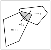
Figure 14: Collision between two floes. The contact forces are calculated in terms of geometric properties of the overlap area, shown in gray. Here, $\boldsymbol{c}$ represents the center of mass of the overlap area and the normal direction $\boldsymbol{n}^{k}_{i,j}$ is taken normal to the line connecting the two intersection points between the floes.

The tangential force is given by

$$\boldsymbol{f}^{T,k}_{i,j}=c_{i,j}^{k}G\,\Delta t\,v_{i,j}^{k}|\boldsymbol{f}^{N,k}_{i,j}|\boldsymbol{t}_{i,j}^{k},$$ (A.5)

where $c_{i,j}^{k}$ is the length of the chord uniting the two intersection points between floes $i$ and $j$ and $G$ is the shear modulus $G=E/(2(1+\nu))$, defined in terms of Poisson’s ratio $\nu$. The parameter $\Delta t$ is the simulation’s time step, $v_{i,j}^{k}$ the tangential velocity difference between both floes, and $\boldsymbol{t}_{i,j}^{k}$ the tangential direction. The tangential force is limited to the following upper bound:

$$|\boldsymbol{f}^{T,k}_{i,j}|\leq\mu^{\ast}|\boldsymbol{f}^{N,k}_{i,j}|,$$ (A.6)

where $\mu^{\ast}$ is the inter-floe friction coefficient.

A.2 Spatial averaging of data

To average the DEM data in space, we must grid the square domain. Taking into account the one dimensional nature of the problem, we divide the domain into $N=10$ cells that stretch in the $x$-direction, such that the edges separating these cells are defined along $N+1$ equispaced points $(y_{0},y_{1},...,y_{N})$ in the $y$-direction. Hence, the resulting grid consists in the cells $[0,L]\times[y_{i-1},y_{i}]$ for $i=1,...,N$, as depicted in figure 15. At each time step, we compute the horizontal velocity $u$ and the components of the stress tensor $\boldsymbol{\sigma}$ by spatially averaging the velocities and stresses of the ice floes contained in each region (the manner in which the stress tensor $\sigma$ is computed for each ice floe is explained in above in appendix A.1. In particular, for each cell of the grid, we perform a mass-weighted averaging such that, for ice floes that are only partially contained in the cell, only the mass of the floe inside the cell is considered. More information about the averaging can be found in Manucharyan and Montemuro, (2022). In order to be consistent with (2.15b), for each run we extract a single pressure $p=\frac{1}{2}(\sigma_{xx}+\sigma_{yy})$ by spatially averaging this quantity over the whole domain.

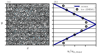
Figure 15: The values of the horizontal velocity $u$ and the stress tensor $\boldsymbol{\sigma}$ are extracted from the DEM data for each time step by averaging spatially over the 10 regions, elongated in the $x$-direction, shown here. In this figure, $n=2000$, $u_{o,max}=2\,$\mathrm{m}$/$\mathrm{s}$$, and $A_{0}=0.8$.

By performing the spatial and temporal averaging, for each DEM computation we obtain a pressure $p\in\mathbb{R}$ and the vectors $(u_{i})$, $(\sigma_{xy,i})$, and $(A_{i})$ of data points in $\mathbb{R}^{N}$. To compute the inertial numbers $I$, we first find the strain rate vector $(\mathrm{d}u_{i})$ via central finite differences, such that $\mathrm{d}u_{i}=(u_{i+1}-u_{i-1})/(2(y_{i+1}-y_{i-1}))$. Then, $I_{i}=\overline{d}\sqrt{H\rho_{i}/p}|\mathrm{d}u_{i}|$, with $\overline{d}=\sqrt{AoL^{2}/n}$.

Appendix B Existence and uniqueness of solutions to the momentum equation

Since the momentum equation (4.8) of the continuous model is equivalent to the minimization of the functional $\mathcal{J}$ over the space $V$, defined in (4.5), it suffices to show that $\mathcal{J}$ admits a unique minimizer to prove the existence and uniqueness of solutions to the momentum equation. To do so, we first write the functional $\mathcal{J}:V\to\mathbb{R}$ as follows for simplicity:

$$\mathcal{J}(v)=\gamma_{1}\left|v\right|_{1}+\gamma_{2}\left|v\right|^{2}_{2}+\gamma_{3}\|u_{o}-v\|_{3}^{3},$$ (B.1)

where $\gamma_{i}>0$ for $i=1,2,3$ are constants and, for $q\geq 1$, $\|\cdot\|_{q}$ and $\left|\cdot\right|_{q}$ are the Sobolev norm and semi-norms, respectively, for the $L^{q}((0,1))$ and $W^{1,q}((0,1))$ spaces; more precisely, these are defined by

$$\|v\|_{q}=\left(\int_{0}^{1}\left|v\right|^{q}\,\mathrm{d}x\right)^{1/q}\quad\text{and}\quad\left|v\right|_{q}=\left(\int_{0}^{1}\left|\frac{\mathrm{d}v}{\mathrm{d}x}\right|^{q}\,\mathrm{d}x\right)^{1/q}.$$ (B.2)

We first remark that $\mathcal{J}$ is well defined for all $v\in V$ by the Sobolev embedding theorem, which implies that $\|v\|_{3}<\infty$. Moreover, for the sake of rigor, we must also assume that $u_{o}\in L^{3}((0,1))$.

According to (Evans,, 2022, theorem 2, chapter 8), at least one function $V$ exists that minimizes $\mathcal{J}$ if the functional is convex and coercive. It is straightforward to check that $\mathcal{J}$ is convex. The functional $\mathcal{J}$ is said to be coercive in $V$ if

$$\|v\|_{V}\to\infty\implies\mathcal{J}(v)\to\infty,$$ (B.3)

where $\|v\|^{2}_{V}=\|v\|_{2}^{2}+|v|_{2}^{2}$. We first note that, by the triangle inequality and Young’s inequality, it follows that

$$\|v\|^{3}_{3}\leq 4\left(\|u_{o}-v\|^{3}_{3}+\|u_{o}\|^{3}_{3}\right).$$ (B.4)

Therefore, for any $v\in V$,

$$\mathcal{J}(v)\geq\gamma_{1}\left|v\right|_{1}+\gamma_{2}\left|v\right|^{2}_{2}+\frac{\gamma_{3}}{4}\|v\|_{3}^{3}-\gamma_{3}\|u_{o}\|_{3}^{3}$$ (B.5)

Using Hölder’s inequality we can show that $\|v\|_{3}\geq\|v\|_{2}$, such that

$$\mathcal{J}(v)\geq\gamma_{2}\left|v\right|^{2}_{2}+\frac{\gamma_{3}}{4}\|v\|_{2}^{3}-\gamma_{3}\|u_{o}\|_{3}^{3},$$ (B.6)

from where coercivity follows. We note that this argument fails whenever $\gamma_{2}=0$, which corresponds with the purely plastic regime, because $\left|v\right|_{1}\to\infty$ does not necessarily follow from $\|v\|_{V}\to\infty$.

To prove that there is only one function that minimizes $\mathcal{J}$, we assume by contradiction that both $u_{1}$ and $u_{2}$ minimize $\mathcal{J}$ and $u_{1}\neq u_{2}$. In this case, we must have that $\mathcal{J}(u_{1})=\mathcal{J}(u_{2})$. We define $w=1/2(u_{1}+u_{2})$ and note that

$$\|u_{o}-w\|_{3}^{3}<\frac{1}{2}\|u_{o}-u_{1}\|_{3}^{3}+\frac{1}{2}\|u_{o}-u_{2}\|_{3}^{3},$$ (B.7)

due to the strict convexity of the function $\|\cdot\|^{3}$ in $\mathbb{R}$ and the injectivity of $\|u_{o}-\cdot\|_{3}^{3}$ in $V$. As a result, by appealing to the convexity of the seminorm $\|\cdot\|_{q}$ for all $q\geq 1$,

$$\mathcal{J}(w)<\frac{1}{2}\mathcal{J}(u_{1})+\frac{1}{2}\mathcal{J}(u_{2})=\mathcal{J}(u_{1}),$$ (B.8)

a contradiction because $\mathcal{J}(u_{1})\leq\mathcal{J}(v)$ for all $v\in V$.

Acknowledgements. We thank Andrew Thompson for many insightful comments and suggestions shared with us during the preparation of the manuscript.

Funding.This work has been supported by the Multidisciplinary University Research Initiatives (MURI) Program, Office of Naval Research (ONR) grant number N00014-19-1-242.

Author contributions. All authors contributed to conceiving and designing the study. GD wrote the paper, designed the figures, performed the simulations and mathematical analysis. MG, SG and GS revised the paper. MG, RH and SG contributed to the simulations, and SG contributed simulation tools. MG, GS and RH provided input to the analysis.

References

- Adams and Fournier, (2003) Adams, R. A. and Fournier, J. J. (2003). Sobolev Spaces. Number 140 in Pure and Applied Mathematics. Academic Press, Elsevier.
- Barker et al., (2015) Barker, T., Schaeffer, D. G., Bohórquez, P., and Gray, J. (2015). Well-posed and ill-posed behaviour of the -rheology for granular flow. Journal of Fluid Mechanics, 779:794–818.
- Bouzid et al., (2013) Bouzid, M., Trulsson, M., Claudin, P., Clément, E., and Andreotti, B. (2013). Nonlocal rheology of granular flows across yield conditions. Physical review letters, 111(23):238301.
- Da Cruz et al., (2005) Da Cruz, F., Emam, S., Prochnow, M., Roux, J.-N., and Chevoir, F. (2005). Rheophysics of dense granular materials: Discrete simulation of plane shear flows. Physical Review E, 72(2):021309.
- Danabasoglu et al., (2020) Danabasoglu, G., Lamarque, J.-F., Bacmeister, J., Bailey, D. A., DuVivier, A. K., Edwards, J., Emmons, L. K., Fasullo, J., Garcia, R., Gettelman, A., Hannay, C., Holland, M. M., Large, W. G., Lauritzen, P. H., Lawrence, D. M., Lenaerts, J. T. M., Lindsay, K., Lipscomb, W. H., Mills, M. J., Neale, R., Oleson, K. W., Otto-Bliesner, B., Phillips, A. S., Sacks, W., Tilmes, S., van Kampenhout, L., Vertenstein, M., Bertini, A., Dennis, J., Deser, C., Fischer, C., Fox-Kemper, B., Kay, J. E., Kinnison, D., Kushner, P. J., Larson, V. E., Long, M. C., Mickelson, S., Moore, J. K., Nienhouse, E., Polvani, L., Rasch, P. J., and Strand, W. G. (2020). The community earth system model version 2 (cesm2). Journal of Advances in Modeling Earth Systems, 12(2):e2019MS001916.
- Dumont, (2022) Dumont, D. (2022). Marginal ice zone dynamics: history, definitions and research perspectives. Philosophical Transactions of the Royal Society A, 380(2235):20210253.
- Evans, (2022) Evans, L. C. (2022). Partial differential equations, volume 19. American Mathematical Society.
- Feltham, (2005) Feltham, D. L. (2005). Granular flow in the marginal ice zone. Philosophical Transactions of the Royal Society A: Mathematical, Physical and Engineering Sciences, 363(1832):1677–1700.
- Feltham, (2008) Feltham, D. L. (2008). Sea ice rheology. Annu. Rev. Fluid Mech., 40:91–112.
- Glowinski et al., (1981) Glowinski, R., Lions, J. L., and Trémoliéres, R. (1981). Numerical Analysis of Variational Inequalities. North Holland.
- Gray and Morland, (1994) Gray, J. M. N. T. and Morland, L. W. (1994). A two-dimensional model for the dynamics of sea ice. Philosophical Transactions of the Royal Society of London. Series A: Physical and Engineering Sciences, 347(1682):219–290.
- Gutfraind and Savage, (1997) Gutfraind, R. and Savage, S. B. (1997). Marginal ice zone rheology: Comparison of results from continuum-plastic models and discrete-particle simulations. Journal of Geophysical Research: Oceans, 102(C6):12647–12661.
- Ham et al., (2023) Ham, D. A., Kelly, P. H. J., Mitchell, L., Cotter, C. J., Kirby, R. C., Sagiyama, K., Bouziani, N., Vorderwuelbecke, S., Gregory, T. J., Betteridge, J., Shapero, D. R., Nixon-Hill, R. W., Ward, C. J., Farrell, P. E., Brubeck, P. D., Marsden, I., Gibson, T. H., Homolya, M., Sun, T., McRae, A. T. T., Luporini, F., Gregory, A., Lange, M., Funke, S. W., Rathgeber, F., Bercea, G.-T., and Markall, G. R. (2023). Firedrake User Manual. Imperial College London and University of Oxford and Baylor University and University of Washington, first edition edition.
- Herman, (2011) Herman, A. (2011). Molecular-dynamics simulation of clustering processes in sea-ice floes. Physical Review E, 84(5):056104.
- Herman, (2022) Herman, A. (2022). Granular effects in sea ice rheology in the marginal ice zone. Philosophical Transactions of the Royal Society A, 380(2235):20210260.
- Hibler III, (1979) Hibler III, W. (1979). A dynamic thermodynamic sea ice model. Journal of physical oceanography, 9(4):815–846.
- Ip et al., (1991) Ip, C. F., Hibler, W. D., and Flato, G. M. (1991). On the effect of rheology on seasonal sea-ice simulations. Annals of Glaciology, 15:17–25.
- Jenkins and Savage, (1983) Jenkins, J. T. and Savage, S. B. (1983). A theory for the rapid flow of identical, smooth, nearly elastic, spherical particles. Journal of fluid mechanics, 130:187–202.
- Jop et al., (2006) Jop, P., Forterre, Y., and Pouliquen, O. (2006). A constitutive law for dense granular flows. Nature, 441(7094):727–730.
- Kamrin and Koval, (2012) Kamrin, K. and Koval, G. (2012). Nonlocal constitutive relation for steady granular flow. Physical review letters, 108(17):178301.
- Manucharyan and Montemuro, (2022) Manucharyan, G. E. and Montemuro, B. P. (2022). Subzero: A sea ice model with an explicit representation of the floe life cycle. Journal of Advances in Modeling Earth Systems, 14(12):e2022MS003247.
- MiDi, (2004) MiDi, G. (2004). On dense granular flows. The European Physical Journal E, 14:341–365.
- Nedderman, (1992) Nedderman, R. M. (1992). Statics and kinematics of granular materials. Cambridge University Press.
- Nicot et al., (2013) Nicot, F., Hadda, N., Guessasma, M., Fortin, J., and Millet, O. (2013). On the definition of the stress tensor in granular media. International Journal of Solids and Structures, 50(14-15):2508–2517.
- Pouliquen et al., (2006) Pouliquen, O., Cassar, C., Jop, P., Forterre, Y., and Nicolas, M. (2006). Flow of dense granular material: towards simple constitutive laws. Journal of Statistical Mechanics: Theory and Experiment, 2006(07):P07020.
- Ringeisen et al., (2023) Ringeisen, D., Losch, M., and Tremblay, L. B. (2023). Teardrop and parabolic lens yield curves for viscous-plastic sea ice models: New constitutive equations and failure angles. Journal of Advances in Modeling Earth Systems, 15(9):e2023MS003613.
- Ringeisen et al., (2019) Ringeisen, D., Losch, M., Tremblay, L. B., and Hutter, N. (2019). Simulating intersection angles between conjugate faults in sea ice with different viscous-plastic rheologies. The Cryosphere, 13(4):1167–1186.
- Rothrock, (1975) Rothrock, D. A. (1975). The energetics of the plastic deformation of pack ice by ridging. Journal of Geophysical Research, 80(33):4514–4519.
- Savage, (1984) Savage, S. B. (1984). The mechanics of rapid granular flows. Advances in applied mechanics, 24:289–366.
- Schaeffer et al., (2019) Schaeffer, D., Barker, T., Tsuji, D., Gremaud, P., Shearer, M., and Gray, J. (2019). Constitutive relations for compressible granular flow in the inertial regime. Journal of Fluid Mechanics, 874:926–951.
- Shen et al., (1987) Shen, H. H., Hibler III, W. D., and Leppäranta, M. (1987). The role of floe collisions in sea ice rheology. Journal of Geophysical Research: Oceans, 92(C7):7085–7096.
- Stewart et al., (2019) Stewart, A. L., Klocker, A., and Menemenlis, D. (2019). Acceleration and overturning of the Antarctic Slope Current by winds, eddies, and tides. Journal of Physical Oceanography, 49(8):2043–2074.
- Wood, (1990) Wood, D. M. (1990). Soil behaviour and critical state soil mechanics. Cambridge university press.
- Zhang and Rothrock, (2005) Zhang, J. and Rothrock, D. A. (2005). Effect of sea ice rheology in numerical investigations of climate. Journal of Geophysical Research: Oceans, 110(C8).