Moscow, Russia
Phase Transition of Anisotropic Hot Dense QGP in Magnetic
Field:
-term Holography for Heavy Quarks
Abstract
We present a five-dimensional twice anisotropic holographic model for heavy quarks supported by Einstein-dilaton-three-Maxwell action. A special feature of the model is the presence of -term in the metric strain coefficient (warp factor). It’s influence on the model properties, mainly on the confinement/deconfinement phase transition, is considered. Conditions for the direct magnetic catalysis are found and the corresponding phase diagrams are discussed.
Keywords:
AdS/QCD, holography, phase transition, Wilson loops, heavy quarks, magnetic field1 Introduction
Theoretical modelling of processes in quark-gluon plasma (QGP) is one of the most vital and urgent problems of quantum chromodynamics (QCD) and high-energy physics in general. Comprehension of QGP phase structure is a step necessary for developing our physical world picture.
To describe the QGP behavior, first of all its confinement/deconfinement phase transition, we use a holographic approach to potential reconstruction method within the AdS5/CFT4 duality Casalderrey-Solana:2011dxg ; Arefeva:2014kyw ; Arefeva:2021kku . Wherein all the important QGP properties should be encoded in the 5D Lagrangian and the metric serving as an ansatz for the corresponding Einstein equations of motion (EOM) solution. This method called a bottom-up approach is broadly applied in high-energy physics for QGP studies Erlich:2005qh ; Karch:2006pv ; Gursoy:2008bu ; Gursoy:2007cb ; Gursoy:2007er ; Gursoy:2009jd ; Andreev:2006nw ; Gursoy:2008za ; Gursoy:2010fj ; Colangelo:2011sr ; Arefeva:2019yzy ; Hajilou:2021wmz ; Li:2013oda ; Li:2012ay ; Mia:2010zu ; Dudal:2018ztm ; Dudal:2017max ; Li:2014dsa ; Yang:2015aia ; Chelabi:2015cwn ; Fang:2015ytf ; Arefeva:2018jyu ; Fang:2018axm ; Chen:2019rez ; He:2013qq ; He:2010ye ; Chen:2018msc and was used in the previous works of our current wide research on holographic QGP (HQGP) AR-2018 ; ARS-2019 ; ARS-2019qfthep ; Arefeva:2019vov ; Arefeva:2019dvl ; Arefeva:2019qen ; APS ; Arefeva:2020aan ; ARS-Light-2020 ; Arefeva:2020vhf ; ARS-Heavy-2020 ; Arefeva:2020bjk ; Arefeva:2021mag ; Arefeva:2021jpa ; Arefeva:2021btm ; Arefeva:2021kku ; Arefeva:2022avn ; Arefeva:2022bhx ; Rannu:2022fxw ; ARS-Light-2022 ; ARS-Heavy-2023 ; Arefeva:2023ter ; Arefeva:2023fky ; Arefeva:2023uji . This consideration is its further development.
It is approved that QGP produced in heavy-ion collisions (HIC) is anisotropic for – fm/ s Strickland:2013uga and exists in strong magnetic field, GeV2 Skokov:2009qp ; Voronyuk:2011jd ; Bzdak:2011yy ; Deng:2012pc . Therefore we include sources of two different anisotropies into the model ansatz: primary anisotropy, representing spacial anisotropy of QGP, and anisotropy associated with magnetic field. We also focus on respectively large values of chemical potential in our consideration, as our research is mainly oriented to future experiments on heavy-ion collisions at high values of baryon density such as NICA project Arefeva:2016rob .
The picture of confinement/deconfinement (phase diagram) actually consists of a combination of two different phase transition types. The 1-st order phase transition originates from the thermodynamical properties of the solution obtained, namely the behavior of free energy as a temperature function, and temporal Wilson loops determining the so called crossover. Both phase transition types are sensible to the quarks mass Brown:1990ev ; Philipsen:2016hkv , with heavy AR-2018 ; ARS-2019 ; ARS-Heavy-2020 ; ARS-Heavy-2023 and light quarks ARS-Light-2020 ; ARS-Light-2022 reacting to magnetic field in different way. Magnetic field also affects heavy and light quarks differently. According to Lattice calculations DElia:2010abb ; DElia:2018xwo ; Bali:2012zg the magnetic catalysis (MC), i.e. the rise of the phase transition temperature with the magnetic field increasing, should take place for heavy quarks, while for light quarks, on the contrary, the phase transition temperature drop with magnetic field increasing, i.e. inverse magnetic catalysis (IMC), is expected.
The quark mass is included into the model effectively via the warp factor exponent. In this work we try to add the -term and investigate it’s effect on the holographic solution properties and the phase diagram features. Such an expansion was proposed in Bohra:2020qom as a promising way to preserve such aspects of QCD in a strong magnetic field as the string tension, the entanglement entropy etc. Our important goal is to improve the magnetic behavior of our previous heavy quarks model ARS-Heavy-2020 .
This paper is organised as follows. In Sect.2 the 5-dim holographic model of hot dense anisotropic QCD in magnetic field is presented and the corresponding 5-dim BH solution reconstructing heavy quarks model is obtained. In Sect.3 thermodynamic properties of the model in magnetic field are considered and the 1-st order phase transition features are revealed. Sect.4 temporal Wilson loops are calculated and the resulting phase diagram is composed. The main conclusions of this investigation and subjects for further research are given in Sect.5. Plots showing the solution behavior are stored in Appendix A. Temperature and free energy dependence on chemical potential and the magnetic field strength are presented on plots in Appendix B.
2 Model
We consider the metric ansatz and the Lagrangian in Einstein frame used in ARS-Heavy-2020 :
| (2.1) | |||
| (2.2) |
| (2.3) |
where and parametrize spacial and magnetic field anisotropies respectively, is the warp factor, is the scalar field, , and are the coupling functions associated with the Maxwell fields , and correspondingly, and are constant “charges” and is the scalar field potential.
Varying Largrangian (2.2) over metric (2.1), the scalar field and vector potential we get the following EOM:
| (2.4) | |||
| (2.5) | |||
| (2.6) | |||
| (2.7) | |||
| (2.8) | |||
| (2.9) | |||
| (2.10) |
Subtracting (2.9) from (2.8) we get the expression for the coupling function :
| (2.11) |
To set a correspondence to Bohra et al. solution Bohra:2020qom we take the warp factor and the coupling function for the electric Maxwell field as
| (2.12) | |||
| (2.13) |
with and . The -term coefficient serves as the model parameter whose effect on the solution properties is investigated.
A B
We solve system (2.4)–(2.11) with usual boundary conditions
| (2.14) | |||
| (2.15) | |||
| (2.16) |
where serves to fit the string tension behavior ARS-Light-2020 , and get
| (2.17) | |||
| (2.18) | |||
| (2.19) |
| (2.20) | |||
| (2.21) | |||
| (2.22) | |||
| (2.23) |
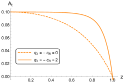
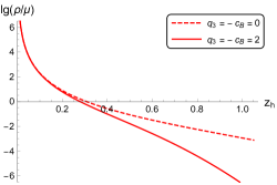
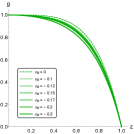
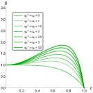
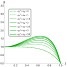
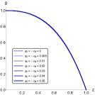
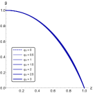
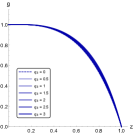
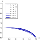
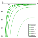
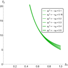
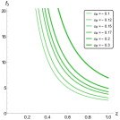
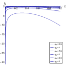
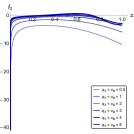
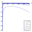
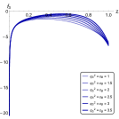
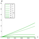
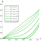
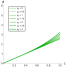
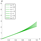
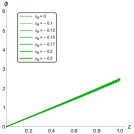
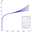
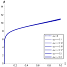
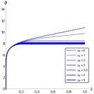
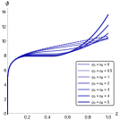
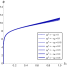
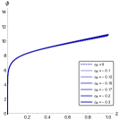
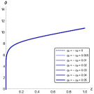
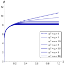
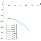
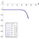
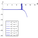
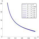
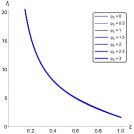
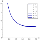
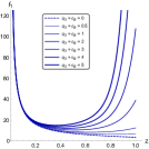
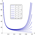
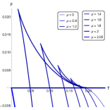
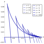
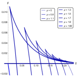
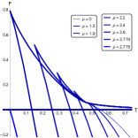
Density is the coefficient in expansion:
| (2.24) |
They both are rather stable relative to magneic field (Fig.1).
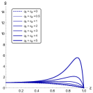
We have two constants describing magnetic field in this model: amount of the magnetic field source and the metric parameter for the magnetic field back-reaction to the 5D curvature. Generally these constants are independent from each other, so different forms of their connection can be possible within the model constructed. Let us now consider the simplest and most obvious set of this connection special cases and check which of them are physical.
Blackening function (Fig.15–16), coupling function (Fig.17–18), scalar field (Fig.19–20) and scalar potenial (Fig.21–22) are plotted in AppendixA. Their analysis is summarised in Table.1, and the main conclusion is that is required.
| , | ||||
|---|---|---|---|---|
| stable stable | NEC noNEC | stable stable | ||
| , | stable unstable | NEC noNEC | stable unstable | |
| stable unstable | noNEC NEC | stable unstable | ||
| stable unstable | NEC noNEC | stable unstable | ||
| stable stable | NEC noNEC | stable stable | ||
| , | stable unstable | NEC noNEC | stable unstable | |
| stable unstable | NEC noNEC | stable unstable | ||
| stable unstable | NEC noNEC | stable unstable |
3 Thermodynamics
A B C D
A B C D
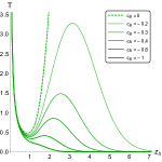
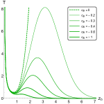
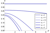
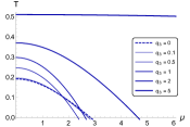
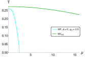
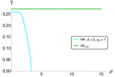
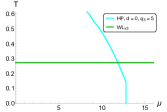
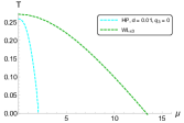
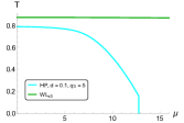
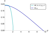
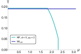
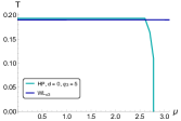
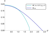
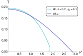
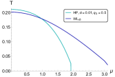
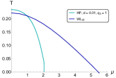
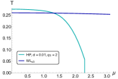
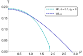
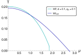
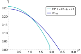
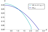
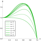
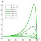
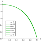
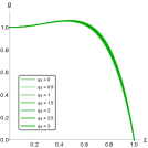
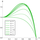
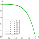
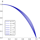
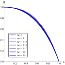
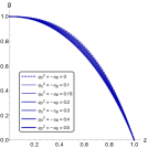
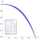
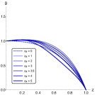
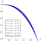
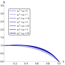
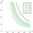
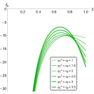
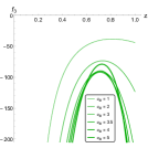
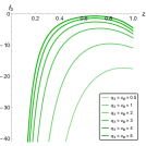
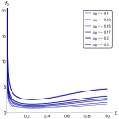
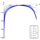
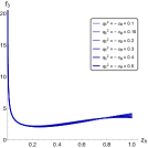
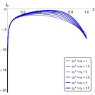
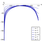
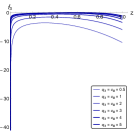
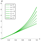
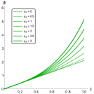
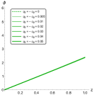
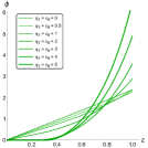
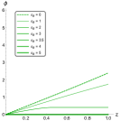
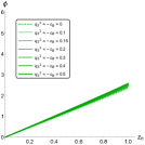
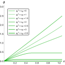
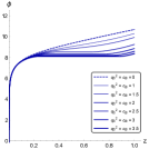
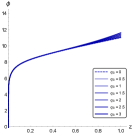
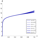
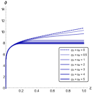
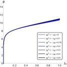
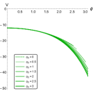
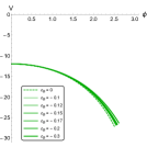
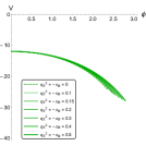
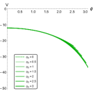
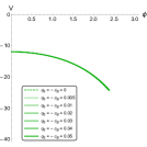
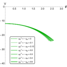
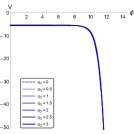
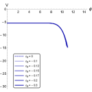
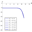
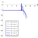
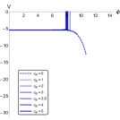
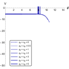
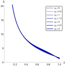
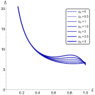
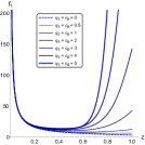
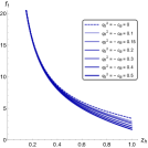
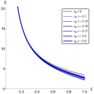
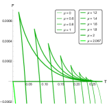
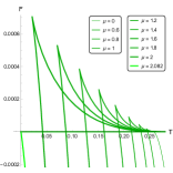
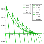
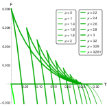
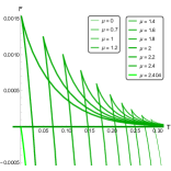
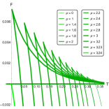
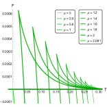
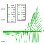
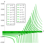
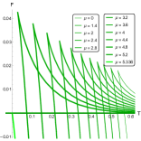
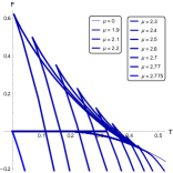
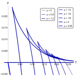
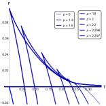
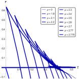
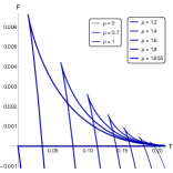
In model Bohra:2020qom type of magnetic catalysis (direct or inverse) depends on coefficient with borderline value . As we look for the magnetic catalysis effect both regions and should be checked. We also try different regimes of undependent and connected and constants. Fig.2–3 show, that direct magnetic catalysis within the current model can be expected for with fixed for both and .
A B C
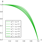
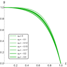
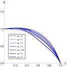
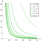
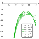
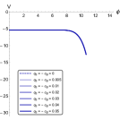
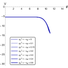
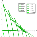
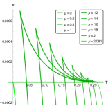
For further investigation we need to choose and fixed values, so let us first consider their influence on thermodynamics properties of the system in primary isotropic case with normalization to the magnetic field . We do not seek for MC effect now (Fig.2.), we are interested in the back-reaction on metric and correction coefficient influence.
A B C
D E F

A B C
D E F
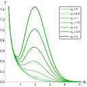
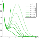
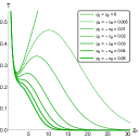
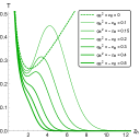
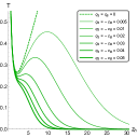
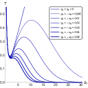
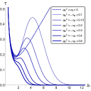
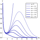
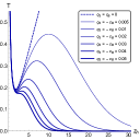
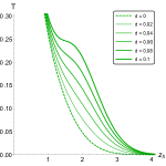
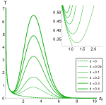
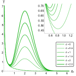
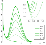
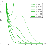
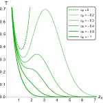
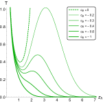
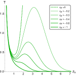
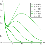
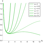
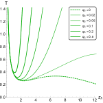
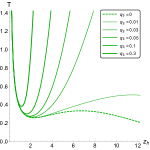
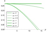
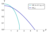
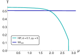
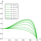
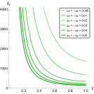
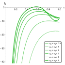
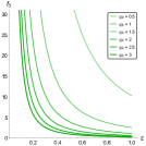
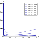
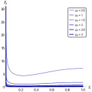
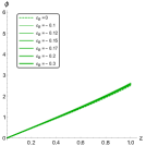
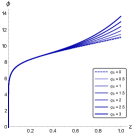
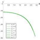
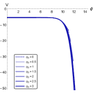
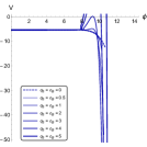
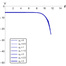
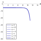
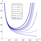
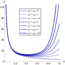
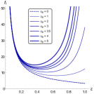
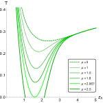
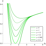
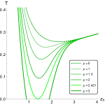
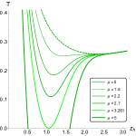
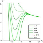
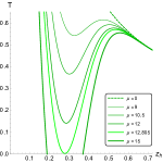
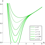
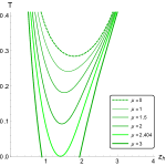
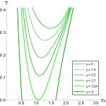
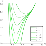
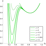
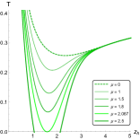
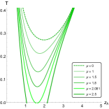
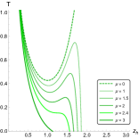
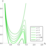
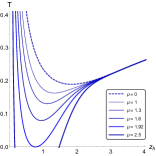
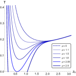
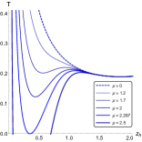
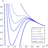
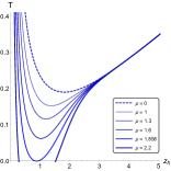
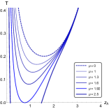
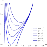
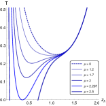
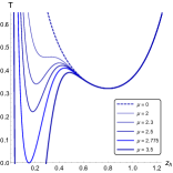
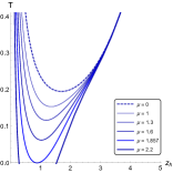
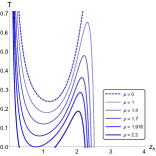
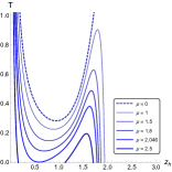
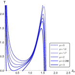
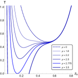
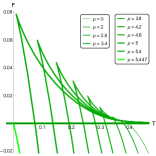
Fig.4 shows the temperature dependence for different back-reaction on metric . It’s larger absolute value, meaning stronger magnetic field influence, makes multivalued temperature behavior degenerate sooner, thus leading to monotony (Fig.4, 1-st line). As to the coefficient , it stabilises the multivalued temperature behavior and consequently the opportunity of the background phase transition. To keep the multivalued behavior within the same interval under stronger magnetic field deformation the larger -value is required (Fig.4, 2-nd line). Besides the local minimum and maximum of temperature are shifted to the left, to the region of lower values by stronger magnetic field deformation, while coefficicient has no notable effect on and positions.
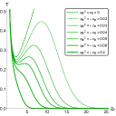
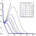
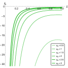
Larger slows down the suppression of the phase transition by magnetic field (Fig.5). Temperature at it’s local maximum and minimum grows and retains multivalued behavior with increasing absolute values of the metric back-reaction .
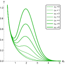
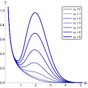
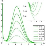
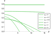
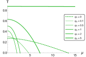
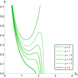
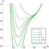
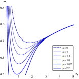
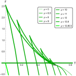
To explore the properties of the current model lets us choose intermediate values of the parameters, so that the magnetic field influence on metric isn’t unlikely weak. On the other hand, we need to preserve zero magnetic field limit, i.e. the 1-st order phase transition should exist at for . Therefore is required (Fig.6.A). Larger makes temperature more sensitive to the magnetic field (Fig.6.B-F), that is especially obvious on small values. Here and futher , and for are considered.
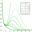
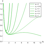
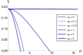
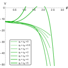
Phase diagram depicts temperature dependence on chemical potential , that, in turn, depends on magnetic field and coefficient . All the plots discussed below are given in Appendix B. In limit temperature has local minimum, whose value decreases with increasing till : (Fig.25.A). For temperature curve splits into two parts, of which only the left one, with smaller , is significant. It decreases monotonously, so the 1-st order phase transition shouldn’t occur any more. As the magnetic field increases, the local minimum for gradually becomes less pronounced and eventually disappears. For larger temperature function is three-valued as the unstable branch corresponding to small black holes (larger ) changes from increasing to decreasing (Fig.25.E.F). Therefore in strong magnetic field the 1-st order phase transition doesn’t exist for near zero and when appears, it has more complex character than usual.
Turning warp factor term on maintains a local temperature minimum even in strong magnetic field (Fig.25). Two-valued function becomes not single-valued, but four-valued instead (Fig.25.F).
In primary isotropic media this particular effect disappears as increases further thus saving 1-st order phase transition for strong magnetic field values (Fig.26.E,F), whereas for intermediate ones it disappears before the transition temperature reaches zero (Fig.26.C,D). Anisotropy doesn’t meet such difficulties (Fig.29.C,D). It also shifts the 1-st order phase transition values down, but doesn’t seem to have a significant effect on other temperature aspects (Fig.27–29).

A B C
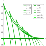
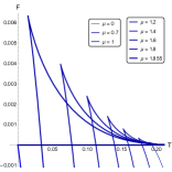
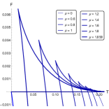
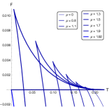
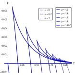
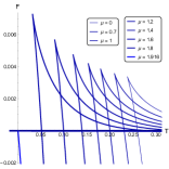
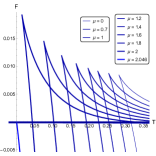
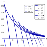
To study phase transition picture a free energy investigation
| (3.3) |
is needed. It confirms the conclusions above regarding the 1-st order phase transition (Fig.30–35). It also shows that the transition mainly occurs from a small black hole to thermal gas, i.e. Hawking-Page phase transition, . The expected exceptions are cases of three- and four-valued temperature for small in strong magnetic field (Fig.30.E,F, 31.E,F, 34.F) and of non-monotonic temperature behavior smoothing for larger in intermediate magnetic field for (Fig.32.C,D).
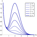
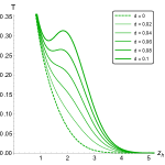
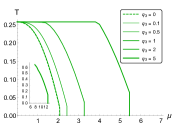
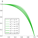
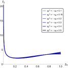
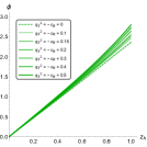
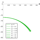
Direct magnetic catalysis is observed for the 1-st order phase transition both in primary isotropic and anisotropic cases (Fig.7). Maximum chemical potential value also increases with magnetic field, but is hardly sensitive to coefficient . For the difference for between zero and non-zero cases is more noticeable for a larger magnetic field (Fig.7, 1-st line), but for it is hardly visible (Fig.7, 2-nd line). Coefficient increases the phase transition temperature and makes the 1-st order phase transition curve decrease not so sharp near the maximum accessible values. This last effect is more significant in anisotropic media .
4 Temporal Wilson loops and phase diagram
To calculate the expectation value of the temporal Wilson loop
| (4.1) |
oriented along vector
| (4.2) |
we use our metric (2.1) as a background:
| (4.3) |
where is the model warp factor in string frame and are the corresponding -metric components.
A B C
We are interested in the turning points for Wilson loops WL, WL and WL, oriented along , and axes, respectively. They are defined by equations:
| (4.4) | |||
| (4.5) | |||
| (4.6) |
These expressions basically are the same that were used in previous considerations ARS-Heavy-2020 ; ARS-Light-2022 , written for the current model’s warp-factor. For the detailed derivation the reader is referred to AR-2018 ; ARS-2019 . In this work we consider WL (4.6) only, as WL (4.4) and WL (4.5) are its particular cases for and .
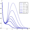
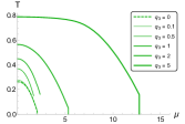
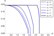
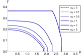
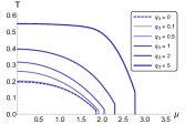
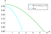
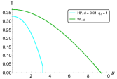
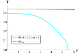
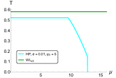
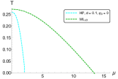
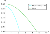
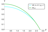
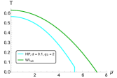
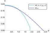
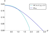
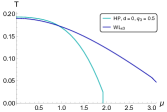
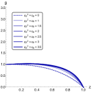
For the phase transition curves provided by the temporal Wilson loops magnetic catalysis effect also takes place (Fig.8). In the limit is the same for any magnetic field, and larger leads to larger temperature along the entire phase transition curve. Its slope decreases with increasing magnetic field and eventually becomes horizontal. As the magnetic field increases, chemical potential range shrinks and then starts to increase again. Together with the curve slope changing this leads to the fact that at large values the phase transition temperature drops for stronger magnetic field, i.e. inverse magnetic catalysis is locally observed. This effect is especially noticeable for primary isotropy (Fig.8, 1-st line) and is quite reduced in anisotropic media (Fig.8, 2-nd line).
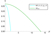
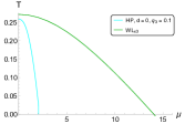
Confronting curves corresponding to the 1-st order phase transition and temporal Wilson loops shows that in primary isotropic media confinement/deconfinement phase transition is completely defined by the 1-st order phase transition (Fig.9–11). The only exception was found for strong magnetic field in limit (Fig.9.F). For a crossover for zero and small is observed, and the crossover region is larger for stronger magnetic field (Fig.12–14).
A B C

D E F

A B C
D E F

A B C
D E F
A B C
D E F
A B C

D E F
A B C
D E F
5 Conslusions
This work investigates the -correction in the holographic warp factor exponent. For this purpose a model describing hot dense anisotropic quarks-gluon plasma in magnetic field is constructed. Spatial anisotropy of the QGP produced in HIC is parametrised by , like it was in previous works. Metric deformation due to magnetic field is described by coefficient. EOM solution requires it to be negative, thus narrowing the possibilities of magnetic catalysis to the only case of fixed and the magnetic field variable .
Via AdS5/CFT4 correspondence the confinement/deconfinement phase transition of QGP in 4D theory is mirrored to the collapse of unstable black hole and presented as the 1-st order phase transition. Free energy consideration shows that it is mainly realised as the Hawking-Page transition of the 5D black hole to thermal gas. Stronger magnetic field leads to the phase transition temperature rise and the chemical potential range expansion. If absolute value is small enough then large magnetic field values can be reached. Isotropisation of the originally anisotropic QGP also leads to larger temperatures and significantly larger available chemical potentials. The effect of direct magnetic catalysis is successfully obtained.
Temporal Wilson loops that are also considered. The corresponding phase transition is presented on the phase diagram as a crossover. It’s temperature and chemical potential range are sensible to magnetic field. But it turns out to take part in the confinement/deconfinement phase transition process for large anisotropy () and loose it’s influence during isotropization. The additional flexibility of this picture is provided by the -term coefficient in the warp factor.
The model obtained in the current work satisfies the stated requirements and it’s fitting capabilities are rather good. At the same time, it needs further researches such as energy losses, string tension, running coupling constant, renormgroup flow behavior and chiral transition.
6 Acknowledgments
The author greatly thanks I. Ya. Aref’eva for fruitful discussions. This work was performed within the scientific project № FSSF-2023-0003 and the “BASIS” Science Foundation, grant № 22-1-3-18-1.
Appendix
Appendix A Solution. Plots
A B

C D
E F
G H

A B
C D
E F

G H

A B
C D
E F


G H

A B
C D

E F

G H
A B
C D
E F


G H
A B

C D

E F
G H


A B


C D
E F


G H

A B
C D
E F

G H

A B
C D
E F


G H
Appendix B Temperature and free energy. Plots
A B C
D E F

A B C
D E F
A B C
D E F

A B C
D E F

A B C
D E F

A B C
D E F
A B C

D E F

A B C
D E F

A B C
D E F
A B C

D E F

A B C
D E F
A B C
D E F
References
- (1) J. Casalderrey-Solana, H. Liu, D. Mateos, K. Rajagopal and U. A. Wiedemann, “Gauge/String Duality, Hot QCD and Heavy Ion Collisions”, Cambridge University Press, 2014, ISBN 978-1-00-940350-4, 978-1-00-940349-8, 978-1-00-940352-8, 978-1-139-13674-7 [arXiv:1101.0618 [hep-th]]
- (2) I. Y. Aref’eva, “Holographic approach to quark–gluon plasma in heavy ion collisions”, Phys. Usp. 57, 527-555 (2014)
- (3) I. Y. Aref’eva, “Theoretical Studies of the Formation and Properties of Quark-Gluon Matter under Conditions of High Baryon Densities Attainable at the NICA Experimental Complex”, Phys. Part. Nucl. 52, 512-521 (2021)
- (4) J. Erlich, E. Katz, D. T. Son and M. A. Stephanov, “QCD and a holographic model of hadrons”, Phys. Rev. Lett. 95, 261602 (2005) [arXiv:hep-ph/0501128 [hep-ph]]
- (5) A. Karch, E. Katz, D. T. Son and M. A. Stephanov, “Linear confinement and AdS/QCD”, Phys. Rev. D 74, 015005 (2006) [arXiv:hep-ph/0602229 [hep-ph]]
- (6) U. Gursoy, E. Kiritsis, L. Mazzanti and F. Nitti, “Deconfinement and Gluon Plasma Dynamics in Improved Holographic QCD”, Phys. Rev. Lett. 101, 181601 (2008) [arXiv:0804.0899 [hep-th]]
- (7) U. Gursoy and E. Kiritsis, “Exploring improved holographic theories for QCD: Part I”, JHEP 02, 032 (2008) [arXiv:0707.1324 [hep-th]]
- (8) U. Gursoy, E. Kiritsis and F. Nitti, “Exploring improved holographic theories for QCD: Part II”, JHEP 02, 019 (2008) [arXiv:0707.1349 [hep-th]]
- (9) U. Gursoy, E. Kiritsis, L. Mazzanti and F. Nitti, “Improved Holographic Yang-Mills at Finite Temperature: Comparison with Data”, Nucl. Phys. B 820, 148-177 (2009) [arXiv:0903.2859 [hep-th]]
- (10) O. Andreev and V. I. Zakharov, “On Heavy-Quark Free Energies, Entropies, Polyakov Loop, and AdS/QCD”, JHEP 04, 100 (2007) [arXiv:hep-ph/0611304 [hep-ph]]
- (11) U. Gursoy, E. Kiritsis, L. Mazzanti and F. Nitti, “Holography and Thermodynamics of 5D Dilaton-gravity”, JHEP 05, 033 (2009) [arXiv:0812.0792 [hep-th]]
- (12) U. Gursoy, E. Kiritsis, L. Mazzanti, G. Michalogiorgakis and F. Nitti, “Improved Holographic QCD”, Lect. Notes Phys. 828, 79-146 (2011) [arXiv:1006.5461 [hep-th]]
- (13) P. Colangelo, F. Giannuzzi, S. Nicotri and V. Tangorra, “Temperature and quark density effects on the chiral condensate: An AdS/QCD study”, Eur. Phys. J. C 72, 2096 (2012) [arXiv:1112.4402 [hep-ph]]
- (14) I. Aref’eva, K. Rannu and P. Slepov, “Cornell potential for anisotropic QGP with non-zero chemical potential”, EPJ Web Conf. 222, 03023 (2019)
- (15) A. Hajilou, “Meson excitation time as a probe of holographic critical point”, Eur. Phys. J. C 83, no.4, 301 (2023) [arXiv:2111.09010 [hep-th]]
- (16) D. Li and M. Huang, “Dynamical holographic QCD model for glueball and light meson spectra”, JHEP 11, 088 (2013) [arXiv:1303.6929 [hep-ph]]
- (17) D. Li, M. Huang and Q. S. Yan, “A dynamical soft-wall holographic QCD model for chiral symmetry breaking and linear confinement”, Eur. Phys. J. C 73, 2615 (2013) [arXiv:1206.2824 [hep-th]]
- (18) M. Mia, K. Dasgupta, C. Gale and S. Jeon, “Heavy Quarkonium Melting in Large N Thermal QCD”, Phys. Lett. B 694, 460-466 (2011) [arXiv:1006.0055 [hep-th]]
- (19) D. Dudal and S. Mahapatra, “Interplay between the holographic QCD phase diagram and entanglement entropy”, JHEP 07, 120 (2018) [arXiv:1805.02938 [hep-th]]
- (20) D. Dudal and S. Mahapatra, “Thermal entropy of a quark-antiquark pair above and below deconfinement from a dynamical holographic QCD model”, Phys. Rev. D 96, no.12, 126010 (2017) [arXiv:1708.06995 [hep-th]]
- (21) D. Li, S. He and M. Huang, “Temperature dependent transport coefficients in a dynamical holographic QCD model”, JHEP 06, 046 (2015) [arXiv:1411.5332 [hep-ph]]
- (22) Y. Yang and P. H. Yuan, “Confinement-deconfinement phase transition for heavy quarks in a soft wall holographic QCD model”, JHEP 12, 161 (2015) [arXiv:1506.05930 [hep-th]]
- (23) K. Chelabi, Z. Fang, M. Huang, D. Li and Y. L. Wu, “Realization of chiral symmetry breaking and restoration in holographic QCD”, Phys. Rev. D 93, no.10, 101901 (2016) [arXiv:1511.02721 [hep-ph]]
- (24) Z. Fang, S. He and D. Li, “Chiral and Deconfining Phase Transitions from Holographic QCD Study”, Nucl. Phys. B 907, 187-207 (2016) [arXiv:1512.04062 [hep-ph]]
- (25) I. Y. Aref’eva, A. A. Golubtsova and G. Policastro, “Exact holographic RG flows and the A1 × A1 Toda chain”, JHEP 05, 117 (2019) [arXiv:1803.06764 [hep-th]]
- (26) Z. Fang, Y. L. Wu and L. Zhang, “Chiral phase transition and QCD phase diagram from AdS/QCD”, Phys. Rev. D 99, no.3, 034028 (2019) [arXiv:1810.12525 [hep-ph]]
- (27) X. Chen, D. Li, D. Hou and M. Huang, “Quarkyonic phase from quenched dynamical holographic QCD model”, JHEP 03, 073 (2020) [arXiv:1908.02000 [hep-ph]]
- (28) S. He, S. Y. Wu, Y. Yang and P. H. Yuan, “Phase Structure in a Dynamical Soft-Wall Holographic QCD Model”, JHEP 04, 093 (2013) [arXiv:1301.0385 [hep-th]]
- (29) S. He, M. Huang and Q. S. Yan, “Logarithmic correction in the deformed model to produce the heavy quark potential and QCD beta function”, Phys. Rev. D 83, 045034 (2011) [arXiv:1004.1880 [hep-ph]]
- (30) J. Chen, S. He, M. Huang and D. Li, “Critical exponents of finite temperature chiral phase transition in soft-wall AdS/QCD models”, JHEP 01, 165 (2019) [arXiv:1810.07019 [hep-ph]]
- (31) I. Ya. Aref’eva and K. A. Rannu, “Holographic Anisotropic Background with Confinement-Deconfinement Phase Transition”, JHEP 05, 206 (2018) [arXiv:1802.05652 [hep-th]]
- (32) I. Ya. Aref’eva, K. A. Rannu and P. S. Slepov, “Orientation dependence of confinement-deconfinement phase transition in anisotropic media”, PLB 792, 470 (2019) [arXiv:1808.05596 [hep-th]]
- (33) I. Aref’eva, K. Rannu and P. Slepov, “Cornell potential for anisotropic QGP with non-zero chemical potential”, EPJ Web Conf. 222, 03023 (2019)
- (34) I. Aref’eva, “Theoretical Studies of Heavy Ion Collisions via Holography”, EPJ Web Conf. 222, 01008 (2019)
- (35) I. Y. Aref’eva, “Holographic Entanglement Entropy for Heavy-Ion Collisions”, Phys. Part. Nucl. Lett. 16, 486-492 (2019)
- (36) I. Y. Aref’eva, “Holographic renormalization group flows”, Theor. Math. Phys. 200, 1313-1323 (2019)
- (37) I. Y. Aref’eva, A. Patrushev and P. Slepov, “Holographic entanglement entropy in anisotropic background with confinement-deconfinement phase transition”, JHEP 07, 043 (2020) [arXiv:2003.05847 [hep-th]]
- (38) I. Y. Aref’eva and K. Rannu, “Holographic Renormalization Group Flow in Anisotropic Matter”, Theor. Math. Phys. 202, 272-283 (2020)
- (39) I. Aref’eva, K. Rannu and P. Slepov, “Holographic Anisotropic Model for Light Quarks with Confinement-Deconfinement Phase Transition”, JHEP 06, 090 (2021) [arXiv:2009.05562 [hep-th]]
- (40) I. Aref’eva, “Holography for Nonperturbative Study of QFT”, Phys. Part. Nucl. 51, 489-496 (2020)
- (41) I. Ya. Aref’eva, K. A. Rannu and P. S. Slepov, “Holographic Anisotropic Model for Heavy Quarks in Anisotropic Hot Dense QGP with External Magnetic Field”, JHEP 07, 161 (2021) [arXiv:2011.07023 [hep-th]]
- (42) I. Y. Aref’eva, K. Rannu and P. Slepov, “Energy Loss in Holographic Anisotropic Model for Heavy Quarks in External Magnetic Field”, [arXiv:2012.05758 [hep-th]]
- (43) I. Y. Aref’eva, K. Rannu and P. S. Slepov, “Anisotropic solutions for a holographic heavy-quark model with an external magnetic field”, Teor. Mat. Fiz. 207, 44-57 (2021)
- (44) I. Y. Aref’eva, A. Ermakov and P. Slepov, “Direct photons emission rate and electric conductivity in twice anisotropic QGP holographic model with first-order phase transition”, Eur. Phys. J. C 82, 85 (2022) [arXiv:2104.14582 [hep-th]]
- (45) I. Y. Aref’eva, K. A. Rannu and P. S. Slepov, “Spatial Wilson loops in a fully anisotropic model”, Teor. Mat. Fiz. 206, 400-409 (2021)
- (46) I. Y. Aref’eva, A. Ermakov, K. Rannu and P. Slepov, “Holographic model for light quarks in anisotropic hot dense QGP with external magnetic field”, Eur. Phys. J. C 83, 79 (2023) [arXiv:2203.12539 [hep-th]]
- (47) I. Y. Aref’eva, K. A. Rannu and P. S. Slepov, “Anisotropic solution of the holographic model of light quarks with an external magnetic field”, Theor. Math. Phys. 210, 363-367 (2022)
- (48) K. Rannu, I. Y. Aref’eva and P. S. Slepov, “Holographic model in anisotropic hot dense QGP with external Magnetic Field”, Rev. Mex. Fis. Suppl. 3, 0308126 (2022)
- (49) I. Y. Aref’eva, A. Ermakov, K. Rannu and P. Slepov, “Holographic model for light quarks in anisotropic hot dense QGP with external magnetic field”, Eur. Phys. J. C 83, no.1, 79 (2023) [arXiv:2203.12539 [hep-th]]
- (50) I. Y. Aref’eva, A. Hajilou, K. Rannu and P. Slepov, “Magnetic catalysis in holographic model with two types of anisotropy for heavy quarks”, Eur. Phys. J. C 83, 1143 (2023) [arXiv:2305.06345 [hep-th]]
- (51) I. Y. Aref’eva, K. A. Rannu and P. S. Slepov, “Dense QCD in Magnetic Field”, Phys. Part. Nucl. Lett. 20, 433-437 (2023)
- (52) I. Y. Aref’eva, “HQCD: HIC in Holographic Approach”, Phys. Part. Nucl. 54 (2023) no.5, 924-930
- (53) I. Y. Aref’eva, “On the quarkyonic phase in the holographic approach”, Theor. Math. Phys. 217 (2023) no.3, 1821-1826
- (54) M. D’Elia, S. Mukherjee and F. Sanfilippo, “QCD Phase Transition in a Strong Magnetic Background”, Phys. Rev. D 82, 051501 (2010) [arXiv:1005.5365 [hep-lat]]
- (55) M. D’Elia, F. Manigrasso, F. Negro and F. Sanfilippo, “QCD phase diagram in a magnetic background for different values of the pion mass”, Phys. Rev. D 98, 054509 (2018) [arXiv:1808.07008 [hep-lat]]
- (56) G. S. Bali, F. Bruckmann, G. Endrodi, Z. Fodor, S. D. Katz and A. Schafer, “QCD quark condensate in external magnetic fields”, Phys. Rev. D 86, 071502 (2012) [arXiv:1206.4205 [hep-lat]]
- (57) M. Strickland, “Thermalization and isotropization in heavy-ion collisions”, Pramana 84, 671-684 (2015) [arXiv:1312.2285 [hep-ph]]
- (58) V. Skokov, A. Y. Illarionov and V. Toneev, “Estimate of the magnetic field strength in heavy-ion collisions”, Int. J. Mod. Phys. A 24, 5925-5932 (2009) [arXiv:0907.1396 [nucl-th]]
- (59) V. Voronyuk, V. D. Toneev, W. Cassing, E. L. Bratkovskaya, V. P. Konchakovski and S. A. Voloshin, “(Electro-)Magnetic field evolution in relativistic heavy-ion collisions”, Phys. Rev. C 83, 054911 (2011) [arXiv:1103.4239 [nucl-th]]
- (60) A. Bzdak and V. Skokov, “Event-by-event fluctuations of magnetic and electric fields in heavy ion collisions”, Phys. Lett. B 710, 171-174 (2012) [arXiv:1111.1949 [hep-ph]]
- (61) W. T. Deng and X. G. Huang, “Event-by-event generation of electromagnetic fields in heavy-ion collisions”, Phys. Rev. C 85, 044907 (2012) [arXiv:1201.5108 [nucl-th]]
- (62) I. Aref’eva, “Holography for Heavy Ions Collisions at LHC and NICA”, EPJ Web Conf. 164, 01014 (2017) [arXiv:1612.08928 [hep-th]]
- (63) F. R. Brown, F. P. Butler, H. Chen, N. H. Christ, Z. h. Dong, W. Schaffer, L. I. Unger and A. Vaccarino, “On the existence of a phase transition for QCD with three light quarks”, Phys. Rev. Lett. 65, 2491-2494 (1990)
- (64) O. Philipsen and C. Pinke, “The QCD chiral phase transition with Wilson fermions at zero and imaginary chemical potential”, Phys. Rev. D 93, 114507 (2016) [arXiv:1602.06129 [hep-lat]]
- (65) H. Bohra, D. Dudal, A. Hajilou and S. Mahapatra, “Chiral transition in the probe approximation from an Einstein-Maxwell-dilaton gravity model”, Phys. Rev. D 103 no.8, 086021 (2021) [arXiv:2010.04578 [hep-th]]