Sampling

Exploiting Spatial and Temporal Correlations in Massive MIMO Systems Over Non-Stationary Aging Channels

Abstract

This work investigates a multi-user, multi-antenna uplink wireless system, where multiple users transmit signals to a base station. Previous research has explored the potential for linear growth in spectral efficiency by employing multiple transmit and receive antennas. This gain depends on the quality of channel state information and uncorrelated antennas. However, spatial correlations, arising from closely-spaced antennas, and channel aging effects, stemming from the difference between the channel at pilot and data time instances, can substantially counteract these benefits and degrade the transmission rate, especially in non-stationary environments. To address these challenges, this work introduces a real-time beamforming framework to compensate for the spatial correlation effect. A channel estimation scheme is then developed, leveraging temporal channel correlations and considering mobile device velocity and antenna spacing. Subsequently, an expression approximating the average spectral efficiency is obtained, dependent on pilot spacing, pilot and data powers, and beamforming vectors. By maximizing this expression, optimal parameters are identified. Numerical results reveal the effectiveness of the proposed approach compared to prior works. Moreover, optimal pilot spacing remains unaffected by interference components such as path loss and the velocity of interference users. The impact of interference components also diminishes with an increasing number of transmit antennas.

I Introduction

In the past two decades, the integration of multiple antennas at both the transmitter and receiver nodes has emerged as a crucial advancement, offering significant advantages in achieving high spectral efficiency (SE) [1, 2, 3, 4, 5, 6, 7]. Notably, massive multiple input multiple output (MIMO) technology, characterized by a substantial number of antennas at the base station (BS), enhances the coverage and SE in the uplink of wireless communications. The studies by [2, 1] underscore a linear growth in ergodic capacity with the number of transmit antennas compared to the single transmit antenna case, and this linear gain is shown to be achieved in high signal-to-interference-plus-noise ratio (SINR) regimes with uncorrelated transmit and receive antennas and when perfect channel state information at the transmitter (CSIT) is available [7, 8, 9].

Furthermore, the correlation between transmit antennas in uplink communications due to insufficient antenna spacing in small mobile devices can substantially degrade the SE. This necessitates optimal signal design strategies at the transmitter. Beamforming, a scalar coding strategy where the transmit covariance matrix is unit-rank, has been identified as one solution. In beamforming, the symbol stream undergoes coding and multiplication by different coefficients at each antenna before transmission. In the context of multi-user multiple input multiple output (MU-MIMO), studies such as [1] demonstrate that user-specific beamforming achieves the sum-capacity with partial channel side information, as discussed by [4, 10].

In a single-antenna uplink scenario within a multi-cellular environment, works such as [11, 12, 8] suggest that linear decoders and precoders behave nearly optimally. Notably, the impact of intra-cell interference diminishes as the number of BS antennas becomes sufficiently large. Additionally, some studies have derived deterministic approximations of SINR for uplink scenarios with maximum ratio combining (MRC) and minimum mean squared error (MMSE) receivers under block-fading channel assumptions, assuming that the number of BS antennas and users tends to infinity at the same rate.

While the advantages highlighted in the mentioned studies concerning multiple antennas are evident, these benefits depend critically on the perfect knowledge of the channel at the transmitter, emphasizing the crucial role of CSIT as noted in [7].

However, existing models often assume block-fading, where the channel remains constant during training and data times, a condition that may not hold in practice, particularly in non-stationary wireless channels as modeled in [13, 14, 15, 16, 17, 18, 19, 20]. Furthermore, due to the relative movement of mobile users in wireless communications, delayed CSIT known as channel aging may occur, resulting from changes in the channel at pilot and data time slots. Neglecting this channel aging effect can negatively impact the capacity of massive MU-MIMO systems, motivating several papers to leverage temporal correlation structures to improve channel estimates [21, 22, 23, 24, 25, 26, 27, 28, 29, 30].

Studies exploring the impact of channel aging, such as [25, 29, 30], have introduced closed-form expressions for the deterministic equivalent SINR under channel aging, considering single input multiple output (SIMO) uplink and multiple input singl output (MISO) downlink scenarios. The inherent challenges of pilot spacing and frame size dimensioning, discussed in [31, 32, 29], highlight the need to balance the resources for channel state information at the receiver (CSIR) acquisition and communication in the presence of channel aging, considering power budgets and evolving channel characteristics.

Motivated by these insights and utilizing tools from random matrix theory, this paper introduces an asymptotically tight deterministic expression for the average SE in the MU-MIMO scenario, featuring multiple antennas at both uplink users and the BS. The proposed framework capitalizes on the temporal dynamics of the channel within a multi-user context, emphasizing the importance of tailored CSIT acquisition for MIMO systems operating over non-stationary wireless channels. Specifically, the emphasis lies in the uplink of a MU-MIMO system, where each user possesses multiple antennas within non-stationary aging channels. Delving into the intricate trade-offs related to imperfect channel knowledge, temporal correlation, and channel aging contributes to a holistic understanding of MIMO system performance in dynamic (and specifically non-stationary) wireless environments. Furthermore, the paper establishes a real-time beamforming framework to harness the evolving nature of both spatial and temporal correlations. Numerical experiments show the efficacy of the proposed approach in exploiting both spatial and temporal correlations.

I-A Contributions and Key Differences with Prior Works

We summarize the contributions of this paper in the following list:

1. Deterministic spectral efficiency in MU-MIMO systems: We propose an explicit expression that reflects the average spectral efficiency in multi-antenna case. Specifically, we first use concentration inequalities derived from tools in random matrix theory to show that the spectral efficiency revolves around its expectation as long as the number of BS antennas is sufficiently large. Next, we obtain a deterministic equivalent expression for the spectral efficiency that approximates the average spectral efficiency. Deriving the deterministic spectral efficiency in scenarios with multiple transmit antennas in MIMO channels poses significant challenges, requiring different strategies compared to the single transmit antenna case explored in, for instance, [30, 29, 8].

2. Optimal beamforming design for enhanced spectral efficiency: To leverage the advantages of employing multiple antennas at the transmitter, we investigate a beamforming vector designed to reshape the data symbols. The determination of optimal beamforming vectors involves maximizing the per-slot deterministic spectral efficiency. We find a closed-form relation for the optimal real-time beamformer. The utilization of these optimal beamformers significantly enhances the resulting deterministic equivalent spectral efficiency.

3. Optimal frame design and power allocation: We propose an optimization framework aimed at maximizing the proposed deterministic-equivalent averaged spectral efficiency while satisfying some power constraints. This endeavor involves identifying optimal values for parameters such as the number of frames, frame sizes, pilot and data powers.

4. Proposing a new algorithm for resource optimization By utilizing an alternative optimization technique and employing steepest ascent, we introduce an effective algorithm for the optimization of transmitter parameters, including pilot spacing, pilot and data powers, and beamformers.

5. Transmitter-centric optimization approach: Our findings indicate that interference components, such as path loss and Doppler frequencies, do not exert an influence on the deterministic equivalent spectral efficiency when a large number of transmit antennas are employed. Additionally, interference components do not impact the optimal frame design, suggesting that all optimization tasks related to frame design can be performed at the transmitter. This eliminates the necessity of transmitting optimal parameters through feedback control loops from the receiver to the transmitter, as discussed in [25, 29]. In scenarios without incorporating transmit beamforming design and with single-antenna users, as discussed in [30], interference may adversely affect the deterministic spectral efficiency. While previous works, including [29, 31, 32], advocate for achieving optimal pilot spacing at the receiver side and transmitting optimal values to the transmitter through feedback or control loops, it is essential to acknowledge that this approach may waste resources and make delays leading to the potential reduction in spectral efficiency.

6. Closed-form expressions for the correlation matrix in MIMO channels: We formulate explicit closed-form expressions for the correlation matrix needed for MIMO channels. Our findings demonstrate that these expressions are accessible in practical non-stationary MIMO time-varying environments. Specifically, in stationary environments, the derived formulas explicitly rely on the spacing between transmit and receive antenna elements, as well as the velocity of users.

I-B Outline

The paper is organized as follows. In Section II, we state the considered model and assumptions for the channel provided in Section II-A and for the uplink pilot and data model provided in Section II-B. In Section III, we have specified the roadmap to obtain the instantaneous SINR and finally we propose an alternative deterministic expression based on random matrix theory tools that concentrates around the random SINR. In Section III, we propose a novel optimization problem that takes into account this deterministic SE and finds the optimal values of beamforming vectors, frame sizes, number of frames and pilot and data powers. Moreover, we propose a heuristic algorithm to find the optimal values of frame size, number of frames and pilot and data powers. Finally, the paper is concluded in Section V.

I-C Notation

$\mathbf{I}_{N}$ denotes the identity matrix of size $N$. vec stands for the column stacking vector operator that transforms a matrix $\mathbf{X}\in\mathbb{C}^{M\times N}$ into its vectorized version $\mathbf{x}\mathbin{\setstackgap{S}{0pt}\stackMath\Shortstack{\smalltriangleup\\ =}}\textbf{vec}(\mathbf{X})\in\mathbb{C}^{MN\times 1}$. The cross covariance matrix between vectors $\mathbf{x}$ and $\mathbf{y}$ is shown by $\mathbf{C}_{\mathbf{x},\mathbf{y}}\mathbin{\setstackgap{S}{0pt}\stackMath\Shortstack{\smalltriangleup\\ =}}\mathds{E}\Big{\{}(\mathbf{x}-\mathds{E}(\mathbf{x}))(\mathbf{y}-\mathds{E}(\mathbf{y}))^{\rm H}\Big{\}}$. The auto-covariance of a random vector $\mathbf{x}$ is shown by $\mathbf{C}_{\mathbf{x}}\mathbin{\setstackgap{S}{0pt}\stackMath\Shortstack{\smalltriangleup\\ =}}\mathds{E}\Big{\{}(\mathbf{x}-\mathds{E}(\mathbf{x}))(\mathbf{x}-\mathds{E}(\mathbf{x}))^{\rm H}\Big{\}}$. $\mathbf{e}_{k}\in\mathbb{R}^{N}$ refers to a vector that has all components equal to zero except for the $k$-th component. $\mathbf{1}_{N}\in\mathbb{R}^{N\times 1}$ is an all-one vector of size $N$. $j\mathbin{\setstackgap{S}{0pt}\stackMath\Shortstack{\smalltriangleup\\ =}}\sqrt{-1}$ is the imaginary unit. $\lambda_{\max}(\mathbf{A})$ stands for the maximum eigenvalue of the matrix $\mathbf{A}$. $[\mathbf{A}]_{k,l}$ is used for the $(k,l)$-th element of the matrix $\mathbf{A}$. $J_{0}(\cdot)$ is the Bessel function of zero kind and is defined as $J_{0}(x)\mathbin{\setstackgap{S}{0pt}\stackMath\Shortstack{\smalltriangleup\\ =}}\tfrac{1}{2\pi}\int_{-\pi}^{\pi}{\rm e}^{-jx\sin(t)}{\rm d}t$. To simplify notation, throughout the paper, we tag User-1 as the intended user, and will sometimes drop index $k=1$ when referring to the tagged user.

II System Model

We consider an uplink communication system where multiple users with multiple antennas transmit data symbols towards a multi-antenna BS equipped with Uniform Linear Array (ULA) (see Figure 2). The number of antennas employed at each user is denoted by $N_{t}$ and the number of antennas at the BS is denoted by $N_{r}$. The users transmit $M$ data frames with sizes $q_{1},...,q_{M}$ as illustrated in Figure 1. Each frame consists of one pilot (training) time slot for CSIT and the rest is dedicated for data transmission. In what follows, we describe the channel model and the received signal model at pilot and data time slots. We assume that the symbol time $T_{s}$ is set to $1$ without loss of generality.

II-A Channel Model

The channel matrix at time slot $t$ between each user and the BS is denoted by $\mathbf{H}(t)\in\mathbb{C}^{N_{t}\times N_{r}}$ which is in general a complex non-stationary zero mean random process with Rayleigh distribution. The vectorized version of the channel is obtained by stacking the rows below each other in a column and is denoted by $\mathbf{h}\mathbin{\setstackgap{S}{0pt}\stackMath\Shortstack{\smalltriangleup\\ =}}{\rm vec}(\mathbf{H})\in\mathbb{C}^{N\times 1}$ where $N\mathbin{\setstackgap{S}{0pt}\stackMath\Shortstack{\smalltriangleup\\ =}}N_{t}N_{r}$. The covariance matrix of the channel vector is shown by $\mathbf{C}_{\mathbf{h}}(t)\mathbin{\setstackgap{S}{0pt}\stackMath\Shortstack{\smalltriangleup\\ =}}\mathds{E}[{\mathbf{h}}(t){\mathbf{h}}^{H}(t)]$. The cross-covariance of the channel vector and the correlation matrix between times $t_{1}$ and $t_{2}$ are shown by $\mathbf{C}_{\mathbf{h}}(t_{1},t_{2})\mathbin{\setstackgap{S}{0pt}\stackMath\Shortstack{\smalltriangleup\\ =}}\mathds{E}[{\mathbf{h}}(t_{1}){\mathbf{h}}^{H}(t_{2})]$ and $\mathbf{P}(t_{1},t_{2})\mathbin{\setstackgap{S}{0pt}\stackMath\Shortstack{\smalltriangleup\\ =}}\mathbf{C}_{\mathbf{h}}^{-\tfrac{1}{2}}(t_{1})\mathbf{C}_{\mathbf{h}}(t_{1},t_{2})\mathbf{C}_{\mathbf{h}}^{-\tfrac{1}{2}}(t_{2})$, respectively. Assume that $t_{1}$ is the current time and $t_{2}<t_{1}$ is some previous time. The channel at time $t_{1}$ can be explicitly described as a sum of two terms: one is based on the correlation information between times $t_{1}$ and $t_{2}$ and the other is the innovative information of the channel at time $t_{1}$. This is stated in the following mathematical formula [30, Proposition 1]:

$${\mathbf{h}}(t_{1})=\underbrace{\mathbf{A}(t_{1},t_{2}){\mathbf{h}}(t_{2})}_{\textup{Correlation information}}+\underbrace{\mathbf{\xi}(t_{1})}_{\textup{Innovative information}},$$ (1)

where $\mathbf{A}(t_{1},t_{2})\mathbin{\setstackgap{S}{0pt}\stackMath\Shortstack{\smalltriangleup\\ =}}\mathbf{C}_{\mathbf{h}}(t_{1},t_{2})\mathbf{C}_{\mathbf{h}}^{-1}(t_{2})$ $\mathbf{\xi}(t_{1})$ denotes the independent channel information at time $t_{1}$ distributed as a zero mean vector with the covariance matrix

$$\mathbf{\Theta}(t_{1})=\mathbf{C}_{\mathbf{h}}(t_{1})-\mathbf{C}_{\mathbf{h}}(t_{1},t_{2})\mathbf{C}^{-1}_{\mathbf{h}}(t_{2})\mathbf{C}_{\mathbf{h}}(t_{2},t_{1}).$$ (2)

II-B Uplink Pilot and Data Model

We consider $M$ frames $m=1,...,M$ in which frame $m$ consists of $q_{m}$ time slots. The first time slot of each frame is devoted to pilot transmission and the rest is employed to transmit data. Within frame $m$ out of total $M$ frames, each communication user sends $\tau_{p}$ pilot symbols in the first time slot, followed by $q_{m}-1$ data time slots according to Figure 1. Define $\delta_{m}\mathbin{\setstackgap{S}{0pt}\stackMath\Shortstack{\smalltriangleup\\ =}}\sum_{l=1}^{m}q_{l}+1$. As we assumed $T_{s}=1$, the total duration of transmitting all frames is $\delta_{M}-1$. The times slots of frame $m$ are from $\delta_{m-1}$ to $\delta_{m}-1$. User-$k$ transmits each of the $F$ pilot symbols with transmit power $P_{p,k}$, and each data symbol in slot-$i$ with transmit power $P_{d,k}(i),\leavevmode\nobreak\ k=1\ldots K$. Assuming that each user uses a pilot matrix $\mathbf{S}\in\mathbb{C}^{\tau_{p}\times N_{t}}$, the received pilot signal from the tagged user at the BS is in the following form:

$$\mathbf{Y}_{p}(t) =\alpha_{1}\sqrt{P_{p}}\mathbf{H}(t)\mathbf{S}^{\rm T}+\mathbf{N}_{\rm p}(t)\leavevmode\nobreak\ \leavevmode\nobreak\ \in\mathbb{C}^{N_{r}\times\tau_{\rm p}},$$ (3)

where $\alpha_{1}$ denotes large scale fading factor, $P_{p}={P_{p}}_{1}$ denotes the pilot power of the tagged user at each pilot time slot, and $\mathbf{N}(t)\in\mathbb{C}^{N_{r}\times\tau_{\rm p}}$ is the additive white Gaussian noise (AWGN) with element-wise variance $\sigma_{\rm p}^{2}$. It is beneficial to write the equation (3) in a matrix-vector form as follows:

$$\mathbf{y}_{p}(t)\mathbin{\setstackgap{S}{0pt}\stackMath\Shortstack{\smalltriangleup{\\ }=}}\textbf{vec}\left(\mathbf{Y}_{p}(t)\right)=\alpha\sqrt{P_{p}}\overline{\mathbf{S}}\mathbf{h}(t)+\mathbf{n}_{\rm p}(t)\leavevmode\nobreak\ \in\mathbb{C}^{\tau_{\rm p}N_{r}\times 1},$$ (4)

where $\mathbf{y}(t)$, $\mathbf{N}_{p}(t)\in\mathbb{C}^{\tau_{\rm p}N_{r}\times 1}$, $\overline{\mathbf{S}}\mathbin{\setstackgap{S}{0pt}\stackMath\Shortstack{\smalltriangleup\\ =}}\mathbf{I}_{N_{r}}\otimes\mathbf{S}\in\mathbb{C}^{\tau_{\rm p}N_{r}\times N}$ are such that $\overline{\mathbf{S}}^{\rm H}\overline{\mathbf{S}}=\tau_{\rm p}\mathbf{I}_{N_{t}}$ and $\mathbf{h}(t)\mathbin{\setstackgap{S}{0pt}\stackMath\Shortstack{\smalltriangleup\\ =}}{\rm vec}(\mathbf{H}(t))$. We also assume that the pilot power corresponding to each pilot time slot is obtained as $P_{p}=\tfrac{{P_{p}}_{\max}}{M}$, where ${P_{p}}_{\max}$ denotes the maximum pilot power of the tagged user.

At data time slot $i$ of frame $m$, the received signal at the BS can be stated as follows:

$$\scalebox{0.8}{$\mathbf{y}_{\rm d}(i)=\underbrace{{\alpha}\mathbf{H}(i)\mathbf{x}(i)}_{\text{tagged user}}+\underbrace{\sum_{k=2}^{K}\alpha_{k}\mathbf{H}_{k}(i)\mathbf{x}_{k}(i)}_{\text{co-scheduled MU-MIMO users}}$}+\mathbf{n}_{\rm d}(i)\in\mathbb{C}^{N_{r}\times 1},$$ (5)

where $\alpha$ is path loss component, $\mathbf{x}_{k}(i)\mathbin{\setstackgap{S}{0pt}\stackMath\Shortstack{\smalltriangleup\\ =}}\mathbf{w}_{k}^{i}s_{k}(i)\in\mathbb{C}^{N_{t}\times 1}$ is the transmitted signal by the $k$-the user, $s_{k}(i)\in\mathbb{C}^{1\times 1}$ is the transmitted data symbol of user $k$ with transmit data power $P_{d,k}=\mathds{E}[|s_{k}(i)|^{2}]$. $s_{k}(i)\in\mathbb{C}$. $\mathbf{w}_{k}^{i}\in\mathbb{C}^{N_{t}\times 1}$ is the real-time beamforming vector of $k$-th user corresponding to time slot $i$. These beamforming vectors will be later optimized to enhance spectral efficiency. Furthermore, $\mathbf{n}_{\rm d}(i)\leavevmode\nobreak\ \sim\mathcal{CN}\left(\mathbf{0},\sigma_{d}^{2}\mathbf{I}_{N_{r}}\right)$ is the AWGN at the receiver. Here, the data power of each data time slot is obtained as $P_{{\rm d},k}=\tfrac{{P_{{\rm d},k}}_{\max}}{\delta_{M}-1-M}$, where ${P_{{\rm d},k}}_{\max}$ denotes the maximum data power of user $k$. The sum of maximum pilot and data powers should not exceed the total power budget which is denoted by $P_{\rm tot}$.

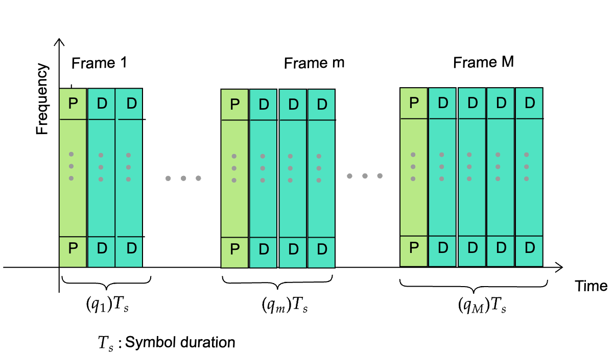
Figure 1: A schematic figure for multi-frame data transmission. $q_{1},...,q_{M}$ specifies the data length of frames $1,...,M$. The first time slot of each frame is considered for pilot transmission and the rest is used for data transmission.

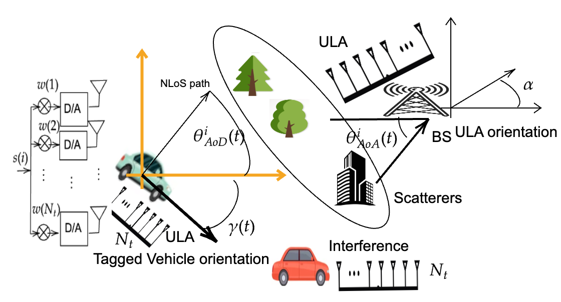
Figure 2: A typical example of multi-antenna multi-user wireless system. Left image: This image shows the beamforming strategy where a single symbol $s(i)$ at time slot $i$ is transmitted simultaneously from $N_{t}$ number of transmit antennas in the tagged user. Right image: This image shows a typical time-varying channel in vehicular networks where there are $L(i)$ number of scatterers between the tagged user and the BS.

III Proposed Scheme

In this section, we provide a road-map of our proposed approach for optimizing beamforming directions, pilot spacing, and power control. First in Section III-A, we propose an explicit link between the velocity of mobile users and the correlation matrix between two different times. Then, we provide a linear MMSE (LMMSE) estimate the time-varying channel as a function of frame size in presence of temporal prior information in Section III-B. Next, in Section III-C, we provide an optimal MMSE receiver combiner for AR channels in order to estimate the date message of the tagged user. Next, in Section III-D, based on channel estimate and data estimate, we calculate the instantaneous slot-by-slot SINR of the tagged user over fast fading non-stationary channels. Then, we state a theorem that provides a deterministic expression for the instantaneous SINR, named deterministic SINR.

III-A Correlation Matrix in MIMO Channels

In this section, we obtain an explicit relation between the correlation matrix that reflects the temporal correlation information of the channel and the velocity of users. A typical example of the considered vehicular network is depicted in the right image of Figure 2. The correlation matrix of the channel is typically influenced by several factors, including the propagation geometry, user’s velocity, and antenna characteristics. As shown in Figure 2, consider the tagged vehicle moving towards direction $\gamma(t)$ at time $t$ with the speed $\nu(t)$. Suppose that the antennas of the BS are aligned in direction $\alpha$ as is shown in Figure 2. The environment between the tagged UE and the BS is composed of $L(t)$ number of scatterers. The angle of departure (AoD) and angle of arrival (AoA) of the $i$-th path at time $t$ are denoted by $\theta_{\rm AoD}^{i}(t)$ and $\theta_{\rm AoA}^{i}(t)$, respectively. Also, the Doppler frequencies of the line of sight (LoS) and non-line of sight (NLoS) paths are obtained by

(6)

where $\lambda\mathbin{\setstackgap{S}{0pt}\stackMath\Shortstack{\smalltriangleup\\ =}}\tfrac{c}{f_{c}}$ is the wavelength of the source, $c=3\times 10^{8}$ and $f_{c}$ is the carrier frequency. The distance between transmit and receive antennas are respectively denoted by $d_{T}$ and $d_{R}$.

Proposition 1.

Assume that the number of scatterers is sufficiently large ($L(t)\rightarrow\infty$) and the AoDs and AoAs are distributed according to some known distributions. Then, the $(N_{t}(p-1)+v,N_{t}(q-1)+w)$ element of the correlation matrix $\mathbf{P}(t_{1},t_{2})\in\mathbb{C}^{N\times N}$ can be obtained as (1).

$$\rho(t_{1},t_{2},p,q,v,w)\mathbin{\setstackgap{S}{0pt}\stackMath\Shortstack{\smalltriangleup{\\ }=}}[\mathbf{P}(t_{1},t_{2})]_{{N_{t}(p-1)+v,N_{t}(q-1)+w}}=$$

$$\mathds{E}\Big{[}{\rm e}^{j\tfrac{2\pi}{\lambda}\big{[}(t_{1}\nu(t_{1})+d_{T}v)\cos(\gamma(t_{1})-\theta_{\rm AoD}(t_{1}))-(t_{2}\nu(t_{2})+d_{T}w)\cos(\gamma(t_{2})-\theta_{\rm AoD}(t_{2}))\big{]}}\Big{]}\mathds{E}\Big{[}{\rm e}^{j\tfrac{2\pi d_{R}}{\lambda}\big{[}p\cos(\alpha-\theta_{\rm AoA}(t_{1}))-q\cos(\alpha-\theta_{\rm AoA}(t_{2}))\big{]}}\Big{]}=I_{1}I_{2}$$ (7)

Proof. See Appendix A.

The formulas provided in (1) can be fully calculated by numerical integration. This model aligns with non-isotropic scattering (more detailed can be found in [13, 33, 34]).

Corollary 1.

(Special cases: Stationary environments and von Mises distribution for AoA and AoD) In the stationary cases where the statistics of the user and environment do not change with time, then the parameters $\nu(t)=\nu,\gamma(t)=\gamma,\theta_{\rm AoA}(t)=\theta_{\rm AoA},\theta_{\rm AoD}(t)=\theta_{\rm AoD}$ are fixed. Define $\tau\mathbin{\setstackgap{S}{0pt}\stackMath\Shortstack{\smalltriangleup\\ =}}t_{2}-t_{1}$ and $n_{R}\mathbin{\setstackgap{S}{0pt}\stackMath\Shortstack{\smalltriangleup\\ =}}q-p,n_{T}\mathbin{\setstackgap{S}{0pt}\stackMath\Shortstack{\smalltriangleup\\ =}}w-v$. Assume that the AoD follows von Mises distribution with the probability density functions given by

(8)

where $\theta^{c}_{AoD}$ is the central AoD and $\kappa_{\rm AoD}$ is a measure of dispersion from central AoD. Similarly, $\theta_{\rm AoA}^{c}$ and $\kappa_{\rm AoA}$ are defined for the AoA. Given these assumptions, the $(N_{t}(p-1)+v,N_{t}(q-1)+w)$ element of the correlation matrix $\mathbf{P}(t_{1},t_{2})$ is obtained as

$$\rho(t_{1},t_{2},p,q,v,w)=I_{1}I_{2},\forall p,q=1,...,N_{r}\leavevmode\nobreak\ \leavevmode\nobreak\ v,w=1,...,N_{t},$$ (9)

where $I_{1}$ and $I_{2}$ are provided in (10).

$$I_{1}=\tfrac{J_{0}(j\sqrt{\kappa_{AoD}^{2}-\tfrac{4\pi^{2}}{\lambda^{2}}(\tau\nu+d_{T}n_{T})^{2}-j\tfrac{4\pi}{\lambda}(\tau\nu+d_{T}n_{T})\kappa_{AoD}\cos(\gamma-\theta^{c}_{AoD})})}{J_{0}(j\kappa_{AoD})},I_{2}=\tfrac{J_{0}(j\sqrt{\kappa_{AoA}^{2}-\tfrac{4\pi^{2}}{\lambda^{2}}n_{R}^{2}d_{R}^{2}+j\tfrac{4\pi}{\lambda}n_{R}d_{R}\kappa_{AoA}\cos(\alpha-\theta^{c}_{AoA})})}{J_{0}(j\kappa_{AoA})}$$ (10)

Corollary 2.

(Special cases: Stationary environment and uniform angles) In the case where the AoD and AoA are distributed uniformly between $[-\pi,\pi]$, we have $\kappa_{\rm AoD}=\kappa_{\rm AoA}=0$ and the $(N_{t}(p-1)+v,N_{t}(q-1)+w)$ element of the correlation matrix $\mathbf{P}(t_{1},t_{2})$ is obtained as

$$\rho(t_{1},t_{2},p,q,v,w)=J_{0}(\tfrac{2\pi}{\lambda}n_{R}d_{R})J_{0}(\tfrac{2\pi}{\lambda}(\tau\nu+d_{T}n_{T})).$$ (11)

In the case of having only single transmit antenna, it holds that $d_{T}=0$ and the relation (11) aligns with the well-established Jakes model provided in [33, Eq. 4] and [34].

III-B LMMSE Channel Estimation with Prior Information

We assume that in each data slot $i$ of frame $m$, the BS utilizes the pilot signals of the current, previous and next frames to estimate the channel in data time slots of the current frame. According to (3), the observed measurements at the pilot time slots corresponding to frames $m-1$, $m$ and $m+1$ are given by :

$$\mathbf{Y}\left(\delta_{m-2}\right)=\alpha_{1}\sqrt{P_{p}}\mathbf{h}\left(\delta_{m-2}\right)\mathbf{S}^{\rm T}+\mathbf{N}_{p}\left(\delta_{m-2}\right),$$

$$\mathbf{Y}\left(\delta_{m-1}\right)=\alpha_{1}\sqrt{P_{p}}\mathbf{h}\left(\delta_{m-1}\right)\mathbf{S}^{\rm T}+\mathbf{N}_{p}\left(\delta_{m-1}\right),$$

$$\mathbf{Y}\left(\delta_{m}\right)=\alpha_{1}\sqrt{P_{p}}\mathbf{h}\left(\delta_{m}\right)\mathbf{S}^{\rm T}+\mathbf{N}_{p}\left(\delta_{m}\right).$$ (12)

By stacking the above relations in matrix-vector form, we have that

$${\mathbf{y}}_{\rm p}\mathbin{\setstackgap{S}{0pt}\stackMath\Shortstack{\smalltriangleup{\\ }=}}\begin{bmatrix}\textbf{vec}(\mathbf{Y}(\delta_{m-2}))\\ \textbf{vec}(\mathbf{Y}(\delta_{m-1}))\\ \textbf{vec}(\mathbf{Y}(\delta_{m}))\end{bmatrix}= \widetilde{\mathbf{S}}{\mathbf{h}_{p}}+{\bm{\epsilon}_{\rm p}}\in\mathbb{C}^{3N_{r}\tau_{\rm p}\times 1},$$ (13)

where ${\mathbf{h}_{p}}=\begin{bmatrix}\mathbf{h}(\delta_{m-2})\\ \mathbf{h}(\delta_{m-1})\\ \mathbf{h}(\delta_{m})\end{bmatrix}\in\mathbb{C}^{3N\times 1}$, $\widetilde{\mathbf{S}}=\mathbf{I}_{3N_{r}}\otimes\mathbf{S}$ and ${\bm{\epsilon}_{\rm p}}\sim\mathcal{CN}(\mathbf{0},\sigma^{2}_{\rm p}\mathbf{I}_{3N_{r}\tau_{\rm p}})$. Note that as a convention, we assumed that $q_{l}=0\leavevmode\nobreak\ \forall l\leq 0$. Having the measurements in pilot time slots provided in (13), one can estimate the channel at data time slot $i$ in frame $m$ as is stated in the following lemma.

Lemma 1.

([30, Lemma 1 and Corrollary 1]) The LMMSE estimate of the channel vector at time slot $i$ of frame $m$ given the measurements $\mathbf{y}_{\rm p}$ in (13) is obtained as

$$\widehat{\mathbf{h}}(i)=\tfrac{1}{\alpha_{1}\sqrt{P_{\rm p}}\tau_{\rm p}}\mathbf{E}(\mathbf{q},i)\left(\mathbf{M}_{m}(\mathbf{q})+\tfrac{\sigma^{2}_{\rm p}}{\alpha_{1}^{2}P_{\rm p}\tau_{\rm p}}\mathbf{I}_{3N_{r}}\right)^{-1}\widetilde{\mathbf{S}}^{\rm H}{\mathbf{y}}_{\rm p},$$ (14)

Moreover, the covariance matrix of the LMMSE channel estimate is provided by:

$$\mathbf{C}_{\widehat{\mathbf{h}}}(i)= \mathbf{E}_{m}(\mathbf{q},i)\left(\mathbf{M}_{m}(\mathbf{q})+\tfrac{\sigma^{2}_{\rm p}}{\tau_{\rm p}\alpha^{2}P_{\rm p}}\mathbf{I}_{3N_{r}}\right)^{-1}\mathbf{E}_{m}^{\rm H}(\mathbf{q},i).$$ (15)

Here,

$$\mathbf{E}_{m}(\mathbf{q},i)\mathbin{\setstackgap{S}{0pt}\stackMath\Shortstack{\smalltriangleup{\\ }=}}{\begin{bmatrix}\mathbf{C}_{\mathbf{h}}(\delta_{m-2},i)&\mathbf{C}_{\mathbf{h}}(\delta_{m-1},i)&\mathbf{C}_{\mathbf{h}}(\delta_{m},i)\end{bmatrix}};$$ (16)

$$\mathbf{M}_{m}(\mathbf{q})\mathbin{\setstackgap{S}{0pt}\stackMath\Shortstack{\smalltriangleup{\\ }=}}$$ (17)

$${\begin{bmatrix}\mathbf{C}_{\mathbf{h}}(\delta_{m-2})&\mathbf{C}_{\mathbf{h}}(\delta_{m-2},\delta_{m-1})&\mathbf{C}_{\mathbf{h}}(\delta_{m-2},\delta_{m})\\ \mathbf{C}_{\mathbf{h}}(\delta_{m-1},\delta_{m-2})&\mathbf{C}_{\mathbf{h}}(\delta_{m-1})&\mathbf{C}_{\mathbf{h}}(\delta_{m-1},\delta_{m})\\ \mathbf{C}_{\mathbf{h}}(\delta_{m},\delta_{m-2})&\mathbf{C}_{\mathbf{h}}(\delta_{m},\delta_{m-1})&\mathbf{C}_{\mathbf{h}}(\delta_{m})\end{bmatrix}}.$$ (18)

III-C MMSE Data Estimate

In this section, we aim to calculate the optimum receiver $\mathbf{g}\in\mathbb{C}^{1\times N_{r}}$ that estimates the transmitted data symbol of the tagged user which is denoted by $s_{1}(i)\in\mathbb{C}$. We assume that the transmitted data vector of the tagged user has zero mean with variance $P_{d,1}$. Specifically, the BS estimates the data transmitted vector of the tagged user at time slot $i$ based on channel estimates provided at $i$ and $i_{p}<i$. The former relies on pilot observation at $i$-th time slot and the latter relies on channel estimate at time slot $i_{p}$ and correlation information between $i_{p}$ and $i$. The following vector collects the channel estimates at time instants $i$ and $i_{p}$: $\bm{\zeta}(i)\mathbin{\setstackgap{S}{0pt}\stackMath\Shortstack{\smalltriangleup\\ =}}\begin{bmatrix}\widehat{\mathbf{h}}(i)\\ \widehat{\mathbf{h}}(i_{p})\end{bmatrix}\in\mathbb{C}^{2N\times 1}.$

Then, the optimum MMSE receiver combiner is provided via the following proposition whose proof is provided in Appendix I of the supplementary material.

Proposition 2.

Let $\mathbf{P}_{\rm c}$ of size $N\times N$ be the commutation matrix which transforms the vectorized version of a matrix to the vectorized version of its transpose. Then, the MMSE optimum receiver given the prior information $\bm{\zeta}(i)$ is obtained as follows:

$$\mathbf{g}^{\star}(i)\mathbin{\setstackgap{S}{0pt}\stackMath\Shortstack{\smalltriangleup{\\ }=}}\mathop{\arg\min}_{\mathbf{g}\in\mathbb{C}^{1\times N_{r}}}\mathds{E}_{s|\bm{\zeta}(i)}|\mathbf{g}\mathbf{y}-s|=\alpha_{1}\sqrt{P_{{\rm d},1}}{\mathbf{w}_{1}^{i}}^{H}\mathbf{J}_{1}^{H}\mathbf{F}(i)^{-1},$$ (19)

where

$$\mathbf{F}(i)\mathbin{\setstackgap{S}{0pt}\stackMath\Shortstack{\smalltriangleup{\\ }=}}\sum_{k=1}^{K}\alpha_{k}^{2}\mathcal{A}_{k}(\mathbf{D}_{k})+\sigma^{2}_{d}\mathbf{I}_{N_{r}},\mathbf{D}_{k}\mathbin{\setstackgap{S}{0pt}\stackMath\Shortstack{\smalltriangleup{\\ }=}}\mathbf{Q}_{k}+\mathbf{z}_{k}\mathbf{z}_{k}^{H},$$ (20)

$$\mathbf{z}_{k}\mathbin{\setstackgap{S}{0pt}\stackMath\Shortstack{\smalltriangleup{\\ }=}}\mathbf{\Psi}_{k}{\bm{\zeta}}_{k}(i),\bm{\zeta}_{k}(i)\mathbin{\setstackgap{S}{0pt}\stackMath\Shortstack{\smalltriangleup{\\ }=}}\begin{bmatrix}&\widehat{\mathbf{h}}_{k}(i)\\ &\widehat{\mathbf{h}}_{k}(i_{p})\end{bmatrix}\in\mathbb{C}^{2N_{t}N_{r}\times 1},$$ (21)

(22)

$$\mathbf{J}_{k}\mathbin{\setstackgap{S}{0pt}\stackMath\Shortstack{\smalltriangleup{\\ }=}}{\rm vec}^{-1}(\mathbf{\Psi}_{k}{\bm{\zeta}}_{k}(i))={\rm vec}^{-1}(\mathbf{z}_{k})\in\mathbb{C}^{N_{r}\times N_{t}},$$ (23)

$$\mathcal{A}_{k}(\mathbf{D}_{k})\mathbin{\setstackgap{S}{0pt}\stackMath\Shortstack{\smalltriangleup{\\ }=}}\begin{bmatrix}\langle{\mathbf{D}^{\prime}}_{k}^{(1,1)},\mathbf{C}_{\mathbf{x}_{k}}\rangle&\ldots&\langle{\mathbf{D}^{\prime}}_{k}^{(1,N_{r})},\mathbf{C}_{\mathbf{x}_{k}}\rangle\\ \vdots&\ddots&\vdots\\ \langle{\mathbf{D}^{\prime}}_{k}^{(N_{r},1)},\mathbf{C}_{\mathbf{x}_{k}}\rangle&\ldots&\langle{\mathbf{D}^{\prime}}_{k}^{(N_{r},N_{r})},\mathbf{C}_{\mathbf{x}_{k}}\rangle\end{bmatrix},$$ (24)

$${\mathbf{D}^{\prime}}_{k}\mathbin{\setstackgap{S}{0pt}\stackMath\Shortstack{\smalltriangleup{\\ }=}}\mathbf{P}_{\rm c}^{H}\mathbf{D}_{k}\mathbf{P}_{\rm c},\mathbf{Q}_{k}\mathbin{\setstackgap{S}{0pt}\stackMath\Shortstack{\smalltriangleup{\\ }=}}\mathbf{C}_{\mathbf{h}_{k}(i)}-\mathbf{\Psi}_{k}\begin{bmatrix}\mathbf{C}_{\widehat{\mathbf{h}}_{k}(i)}\\ \mathbf{C}_{\widehat{\mathbf{h}}_{k}(i_{p})}\mathbf{A}(i,i_{p})^{H}\end{bmatrix},$$ (25)

and $\mathbf{D}_{k}^{(i,j)}\in\mathbb{C}^{N_{t}\times N_{t}}$ is the $(i,j)$ block of matrix $\mathbf{D}_{k}$, i.e.,

$$\mathbf{D}_{k}=\begin{bmatrix}\mathbf{D}_{k}^{{(1,1)}}&\ldots&\mathbf{D}_{k}^{(1,N_{r})}\\ \vdots&\ddots&\ldots\\ \mathbf{D}_{k}^{{(N_{r},1)}}&\ldots&\mathbf{D}_{k}^{(N_{r},N_{r})}\end{bmatrix}.$$ (26)

These results serve as a starting point for deriving the achievable SINR and spectral efficiency in the next subsection.

III-D SINR and SE Calculations

In this section, we will calculate the instantaneous SINR based on channel and data estimates provided in Sections III-B and III-C. The following theorem calculates the instantaneous SINR for the tagged user.

Theorem 1.

Suppose there exists prior information regarding the channel at time $i$, gathered in $\bm{\zeta}(i)$. Additionally, the receiver utilizes the MMSE combiner to estimate the data symbols of the tagged user during time slot $i$. Consequently, the instantaneous SINR of the data symbol for the tagged user at time slot $i$ is derived as follows:

$$\gamma(\mathbf{q},i,\zeta(i))=\alpha^{2}\mathbf{z}_{1}^{\rm H}\left(\mathbf{C}_{\mathbf{x}}\otimes\left(\mathbf{F}(i)-\alpha_{1}^{2}\mathcal{A}_{1}(\mathbf{z}_{1}\mathbf{z}_{1}^{\rm H})\right)^{-1}\right)\mathbf{z}_{1}$$

$$\leavevmode\nobreak\ \leavevmode\nobreak\ \leavevmode\nobreak\ \leavevmode\nobreak\ \leavevmode\nobreak\ \leavevmode\nobreak\ \leavevmode\nobreak\ \leavevmode\nobreak\ \leavevmode\nobreak\ \leavevmode\nobreak\ \leavevmode\nobreak\ \leavevmode\nobreak\ \leavevmode\nobreak\ \mathbin{\setstackgap{S}{0pt}\stackMath\Shortstack{\smalltriangleup{\\ }=}}\alpha_{1}^{2}\mathbf{z}_{1}^{\rm H}\left(\mathbf{C}_{\mathbf{x}}\otimes\mathbf{F}_{1}^{-1}(i)\right)\mathbf{z}_{1},$$ (27)

where $\mathbf{F}_{1}\mathbin{\setstackgap{S}{0pt}\stackMath\Shortstack{\smalltriangleup\\ =}}\mathbf{F}_{1}(i)\mathbin{\setstackgap{S}{0pt}\stackMath\Shortstack{\smalltriangleup\\ =}}\mathbf{F}(i)-\alpha_{1}^{2}\mathcal{A}_{1}(\mathbf{z}_{1}\mathbf{z}_{1}^{\rm H})$.

Proof. See Appendix B.

The latter result immediately leads to finding the random SE as follows:

$$\textup{SE}\Big{(}\mathbf{q},i,\bm{\zeta}(i)\Big{)}\mathbin{\setstackgap{S}{0pt}\stackMath\Shortstack{\smalltriangleup{\\ }=}}\log\Big{(}1+\gamma(\mathbf{q},i,\bm{\zeta}(i))\Big{)},$$ (28)

which is a random variable. In the following theorem, utilizing concentration inequality findings from the tools of random matrix theory, as provided in [35], we provide a deterministic equivalent formulation for the SE. This expression offers a suitable approximation for the average SE in scenarios where the number of BS antennas is sufficiently large.

Theorem 2.

Define $\bm{\Theta}\mathbin{\setstackgap{S}{0pt}\stackMath\Shortstack{\smalltriangleup\\ =}}\sum_{k=1}^{K}\alpha_{k}^{2}\mathcal{A}_{k}(\mathbf{Q}_{k})$ and $\rho_{\rm d}\mathbin{\setstackgap{S}{0pt}\stackMath\Shortstack{\smalltriangleup\\ =}}\sigma_{\rm d}^{2}$. Assume that $\bm{\Psi}_{k}$ and $\mathbf{C}_{\bm{\zeta}_{k}}$ have uniformly bounded spectral norms. Then, when $N_{r}$ is sufficiently large ($N_{r}\rightarrow\infty$), the instantaneous SE provided in (28) is concentrated around a deterministic expression given by:

$${\textup{SE}}^{\circ}(\mathbf{q},i,\mathbf{w}^{i})\mathbin{\setstackgap{S}{0pt}\stackMath\Shortstack{\smalltriangleup{\\ }=}}\log\Bigg{(}1+P_{{\rm d},1}\alpha_{1}^{2}$$

$$\left\langle\mathbf{C}_{\mathbf{z}_{1}},\mathbf{w}^{i}{\mathbf{w}^{i}}^{H}\otimes\left(\sum_{k=2}^{K}\tfrac{\alpha_{k}^{2}\mathcal{A}_{k}(\mathbf{C}_{\mathbf{z}_{k}})}{1+\alpha_{k}^{2}\omega_{k}}+\bm{\Theta}+\rho_{\rm d}\mathbf{I}_{N_{r}}\right)^{-1}\right\rangle\Bigg{)},$$ (29)

where $\omega_{2},\ldots,\omega_{K}$ are the solution of the following system of equations for $k=2,\ldots,K$:

$$\omega_{k}=\left\langle\mathbf{C}_{\mathbf{z}_{k}},\mathbf{C}_{\mathbf{x}_{k}}\otimes\left(\sum_{l=2}^{K}\tfrac{\alpha_{l}^{2}\mathcal{A}_{l}(\mathbf{C}_{\mathbf{z}_{l}})}{1+\alpha_{l}^{2}\omega_{l}}+\bm{\Theta}+\rho_{\rm d}\mathbf{I}_{N_{r}}\right)^{-1}\right\rangle.$$ (30)

Proof. See Appendix C.

The deterministic equivalent SE provided in (2) depends on the beamforming vectors $\mathbf{w}_{1}^{i},...,\mathbf{w}_{K}^{i}$ of size $N_{t}\times 1$. We further find the optimal value of the beamforming vector of the tagged user at time slot $i$ in the following proposition.

Proposition 3.

Partition the matrix $\mathbf{C}_{\mathbf{z}}=\mathbf{C}_{\mathbf{z}_{1}}$ as below:

$$\mathbf{C}_{\mathbf{z}_{1}}=\begin{bmatrix}\mathbf{C}_{\mathbf{z}}^{1,1}&\ldots&\mathbf{C}_{\mathbf{z}}^{1,N_{r}}\\ \vdots&\ddots&\vdots\\ \mathbf{C}_{\mathbf{z}}^{N_{r},1}&\ldots&\mathbf{C}_{\mathbf{z}}^{N_{r},N_{r}}\end{bmatrix}.$$ (31)

Define the linear operator $\mathcal{G}(\cdot):\mathbb{C}^{N\times N}\rightarrow\mathbb{C}^{N_{t}\times N_{t}}$ as

$$\mathcal{G}(\mathbf{C}_{\mathbf{z}_{1}})=\sum_{i,l=1}^{N_{r}}\Phi(i,l)\mathbf{C}_{\mathbf{z}_{1}}^{i,l},$$ (32)

where

$$\bm{\Phi}\mathbin{\setstackgap{S}{0pt}\stackMath\Shortstack{\smalltriangleup{\\ }=}}\left(\sum_{k=2}^{K}\tfrac{\alpha_{k}^{2}\mathcal{A}_{k}(\mathbf{C}_{\mathbf{z}_{k}})}{1+\alpha_{k}^{2}\omega_{k}}+\bm{\Theta}+\rho_{\rm d}\mathbf{I}_{N_{r}}\right)^{-1}\in\mathbb{C}^{N_{r}\times N_{r}}.$$ (33)

Then, the optimal real-time beamformer ${{\mathbf{w}}^{i}}^{\star}$ that maximizes the deterministic equivalent SE provided in (2) is the eigenvector of $\bm{\Phi}$ that corresponds to the maximum eigenvalue of $\bm{\Phi}$.

Proof. See Appendix D.

In what follows, we provide an optimization problem that finds the optimal values of $M$, $q_{m}$, ${P_{\rm p}}_{\max}$ and ${P_{\rm d}}_{\max}$. The objective function that we use is obtained by replacing the optimal ${{\mathbf{w}}^{i}}^{\star}$ into the formula (2) and taking average over all time slots, which is named Detetministic Averaged Spectral Efficiency (DASE), and is given by

$${\rm DASE}=\tfrac{\sum_{l=1}^{\delta_{M}-1}\text{SE}^{\circ}(\mathbf{q},l,{\mathbf{w}^{l}}^{\star})}{\delta_{M}-1}.$$ (34)

By having this objective function, the proposed optimization problem is as follows:

$${\max}_{\mathbf{q},M,{P_{\rm p}}_{\max},{P_{\rm d}}_{\max}}\tfrac{\sum_{l=1}^{\delta_{M}-1}\text{SE}^{\circ}(\mathbf{q},l,{\mathbf{w}^{l}}^{\star})}{\delta_{M}-1},\leavevmode\nobreak\ \leavevmode\nobreak\$$

$${\rm s.t.}\leavevmode\nobreak\ \leavevmode\nobreak\ {P_{\rm p}}_{\max}+{P_{\rm d}}_{\max}\leq P_{\rm tot},$$ (35)

where ${P_{\rm d}}_{\max}={P_{{\rm d},1}}_{\max}$ and ${P_{\rm p}}_{\max}={P_{{\rm p},1}}_{\max}$ denote the maximum data and pilot power of the tagged user, respectively.

Remark 1.

(Critical factors in the proposed optimization problem (III-D).) From the numerical experiments conducted in Section IV, it becomes evident that the Doppler frequency of interference users and the interference path do not influence the determination of optimal frame design ($\mathbf{q}^{\star}$ and $M^{\star}$). Moreover, as the number of transmit antennas increases, the distinctions in the SE of the tagged user under varying interference path loss and Doppler frequencies diminish. This characteristic positions our method as transmitter-centric, allowing for all optimization tasks to be efficiently performed at the transmitter side (user side) rather than the receiver side (BS side).

The optimization problem (III-D) is a non-polynomial time (NP)-hard mixed-integer nonlinear problem. In this section, we present a heuristic algorithm named OptResource for determining the optimal values of frame size, number of frames, and pilot and data powers. The pseudocode for this algorithm is outlined in Algorithm 1. For each number of frames and frame size, an estimation of the beamforming vectors is obtained based on an estimate of the pilot and data powers, using Proposition 3 in Line 10. Subsequently, a projected gradient ascent is employed to identify the optimal values of pilot and data powers (Lines 12 to 19). The projected gradient ascent involves two steps: the update step and projection. In the update step (Line 15), a regular gradient ascent is performed. However, the resulting power variables after this step may fall outside the feasible region (where the sum of pilot and power must be less than the total power budget). To address this, the updated power variables are projected in Line 17 to the nearest point within the feasible region. After determining the optimal pilot and data powers, Line 10 is again used to update the beamforming, and an alternative optimization (AO) approach is applied to jointly find the optimum beamforming and powers. The algorithm iterates through all possible values of $M$ and $q_{m}$ to identify the combination leading to the maximum spectral efficiency. The final outputs of OptResource are $\mathbf{q}^{\star},M^{\star},{P_{p}}_{\max}^{\star},{P_{d}}_{\max}^{\star},\mathbf{W}_{\rm B}^{\star}=[{\mathbf{w}^{1}}^{\star},...,{\mathbf{w}^{\delta_{M^{\star}}-1}}^{\star}]$.

Algorithm 1 Proposed algorithm for resource optimization in MIMO systems

1:procedure OptResource($\mathbf{P}(t_{1},t_{2})$, $\rm Tol$, $\mathbf{q}_{\max}$, $M_{\max}$, ${\rm maxiter}$, ${\rm maxiter}_{\rm AO}$, $P_{\rm tot}$)

2:     Define $\bm{\varrho}\mathbin{\setstackgap{S}{0pt}\stackMath\Shortstack{\smalltriangleup\lx@algorithmicx@@item=}}[{P_{p}}_{\max},{P_{d}}_{\max}]^{\rm T},$

4:     Pick an initial point $\bm{\varrho}^{0}$ for maximum pilot and data power that satisfies $\mathbf{1}^{\rm T}\bm{\varrho}^{0}\leq P_{\rm tot}$

5:     $M=1,{\rm SE}^{\star}=0,\bm{\varrho}^{\star}\leftarrow\bm{\varrho}^{0}$

6:     while $M\leq M_{\max}$ do

7:         for $i_{1}=1\leavevmode\nobreak\ {\rm to}\lceil\tfrac{q_{\max}}{M}\rceil$ do

8:              ⋮

9:              for $i_{M}=1\leavevmode\nobreak\ {\rm to}\lceil\tfrac{q_{\max}}{M}\rceil$ do

10:                  for ${\rm it}=1\leavevmode\nobreak\ {\rm to}\leavevmode\nobreak\ {\rm maxiter}_{\rm AO}$ do

11:                       Find an estimate of the beamforming vectors $\mathbf{W}_{\rm B}\mathbin{\setstackgap{S}{0pt}\stackMath\Shortstack{\smalltriangleup\lx@algorithmicx@@item=}}[\mathbf{w}^{1},...,\mathbf{w}^{\delta_{M}-1}]$ by Proposition 3 as follows: $\mathbf{W}_{\rm B}^{\star}\leftarrow\mathop{\arg\max}_{\mathbf{W}_{\rm B}}f_{1}(\bm{\varrho}^{\star},\mathbf{W}_{\rm B})={\rm SE}^{\circ}(\mathbf{q},\bm{\varrho}^{\star},\mathbf{W}_{\rm B})$

13:                       Objective function for power:

14:                       $f(\bm{\varrho})\mathbin{\setstackgap{S}{0pt}\stackMath\Shortstack{\smalltriangleup\lx@algorithmicx@@item=}}{\rm DASE}(i_{1},...,i_{M},M,\bm{\varrho},\mathbf{W}_{\rm B}^{\star})$ in (34)

16:                       $k\leftarrow 1$

17:                       while $\|{\bm{\varrho}}^{k}-{\bm{\varrho}}^{k-1}\|_{2}>\rm Tol$ and $|f({\bm{\varrho}}^{k})-f({\bm{\varrho}}^{k-1})|>\rm Tol$ and $k<{\rm maxiter}$ do Compute ascent direction by calculating $\tfrac{\partial{\rm SE}}{\partial{\bm{\varrho}}}$ at the point ${\bm{\varrho}}^{k}$

18:Update according to $\widetilde{{\bm{\varrho}}}^{k+1}\leftarrow{\bm{\varrho}}^{k}+\alpha\tfrac{\partial{\rm SE}}{\partial{\bm{\varrho}}}$

19:Project to the closest point inside feasible region

20:${\bm{\varrho}}^{k+1}=\mathop{\arg\min}_{\mathbf{x}}\|\mathbf{x}-\widetilde{{\bm{\varrho}}}^{k+1}\|_{2}\leavevmode\nobreak\ \leavevmode\nobreak\ {\rm s.t.}\leavevmode\nobreak\ \mathbf{1}^{\rm T}\mathbf{x}\leq P_{\rm tot}$

21:                           $k\leftarrow k+1$

22:                       end while

23:                       ${\bm{\varrho}}^{\star}\leftarrow{\bm{\varrho}}^{k}$

24:                       $SE=f(\bm{\varrho}^{\star})$

25:                       if $SE>{SE}^{\star}$ then

26:                           ${SE}^{\star}\leftarrow SE$

27:                           $\mathbf{q}^{\star}\leftarrow[i_{1},,...,i_{M}]^{\rm T}$

28:                           $M^{\star}\leftarrow M$

29:                       end if

30:                  end for

31:              end for

32:              ⋮

33:         end for

34:         $M\leftarrow M+1$

35:     end while

36:$[{P_{p}}_{\max}^{\star},{P_{d}}_{\max}^{\star}]^{\rm T}\leftarrow{\bm{\varrho}}^{\star}$

37:end procedure

38:Outputs: $\mathbf{q}^{\star},M^{\star},{P_{p}}_{\max}^{\star},{P_{d}}_{\max}^{\star},\mathbf{W}_{\rm B}^{\star}=[{\mathbf{w}^{1}}^{\star},...,\mathbf{w}^{\delta_{M^{\star}}-1}]$.

IV Numerical Results

In this section, we examine some numerical experiments to evaluate the performance of our proposed method. We consider a Kronecker model for the correlation matrix in all experiments as $\mathbf{P}(t_{1},t_{2})=\mathbf{P}_{\rm T}(t_{1},t_{2})\otimes\mathbf{P}_{\rm R}(t_{1},t_{2})$ where $\mathbf{P}_{\rm T}(t_{1},t_{2})\in\mathbb{C}^{N_{t}\times N_{t}}$ and $\mathbf{P}_{\rm R}(t_{1},t_{2})\in\mathbb{C}^{N_{t}\times N_{t}}$ are the correlation matrices of the transmit and receive antennas, respectively. In the stationary case, we assume in the experiments that $\mathbf{P}_{\rm T}=\rho_{1}\mathbf{1}_{N_{t}}\mathbf{1}_{N_{t}}^{H}+(1-\rho_{1})\mathbf{I}_{N_{t}}$ and $\mathbf{P}_{\rm R}=\rho_{2}\mathbf{1}_{N_{r}}\mathbf{1}_{N_{r}}^{H}+(1-\rho_{2})\mathbf{I}_{N_{r}}$ with $\rho_{1}=0.9,\rho_{2}=0$ which imply that the transmit antennas are close to each other and they are to a great extent correlated and the receive antennas are uncorrelated. In the first experiment, we consider $q_{\max}=6$ and $M_{\max}=3$ and compare three cases in Table I: 1. using one frame with one pilot time slot and $5$ data time slots. 2. using $M=2$ frames with two pilot time slots at the first of each frame. 3. using $M=3$ frames with three pilots. Each of the three rows in Table I corresponds to one experiment. The first four experiments are related to the stationary settings, while the rest examine the performance of our method in non-stationary scenarios. We consider $K=2$ users, where the first user is the tagged user. The Doppler frequencies, pilot power, data power, path loss and channel variances are shown respectively by ${f_{d}}_{i},{{P_{p}}_{i}}_{\max},{{P_{d}}_{i}}_{\max},{\rm PL}_{i},\sigma_{\mathbf{h}_{i}}^{2}$ where $i=1$ corresponds to the tagged user and $i=2$ shows the interference component. The optimal values for the number $M$ of frames, frame size $\mathbf{q}$ and their corresponding DASE are shown by bold numbers. The pilot and data power in this experiment are assumed to be fixed. Note that signal-to-noise ratio (SNR) is defined as ${\rm SNR}=10\log(\tfrac{P_{d}}{\sigma_{d}^{2}})-{\rm PL}_{1}$ where ${\rm PL}_{1}=20\log(\alpha_{1})$ is the path loss of the channel corresponding to the tagged user. Note that the values of both SNR and ${\rm PL}$ are shown in dB unit. The first two experiments shown in the first six rows of Table I compare the single antenna with the multi-antenna case in a scenario where the Doppler frequency of the tagged user is low and our proposed method suggests to use the maximum possible data slots with one frame. However, using multiple antennas leads to higher SE compared to single-antenna case. In the second experiment, shown in the 7th-12th rows of Table I, we examine a scenario where the user is rapidly moving with a high speed in the two cases of $N_{t}=5$ and $N_{t}=1$. We observe that the optimal frame sizes for $N_{t}=5$ occurs in $\mathbf{q}^{\star}=[3,2]$ while in single-antenna case, the optimal frame size is $\mathbf{q}^{\star}=[2,2,2]$. This shows that having multiple antennas at the transmit side not only leads to higher SE but also spends less pilot time slots compared to the single-antenna case. In the last experiment of Table I, we examine a non-stationary scenario where the tagged user is moving with a time-varying speed. We observe that using multiple antennas ($N_{t}=5$) and only one frame with frame size $\mathbf{q}^{\star}=3$ leads to the highest SE, while the optimal design in single-antenna case occurs at $\mathbf{q}^{\star}=[3,2]$. This suggests that in multi-antenna transmitter with optimized beamforming, one can allocate the whole power to data time slots while in single-antenna, the power is distributed in two frames, which requires more pilot time slots to achieve the highest possible SE.

In the second experiment, we investigate the impact of the Doppler effect and the number of transmit antennas and power ratio on the optimal frame design, as illustrated in Figure 3. Here, the power ratio specifies the distribution between pilot and data power, and is defined as ${r_{p}}_{i}=\tfrac{{{P_{p}}_{i}}_{\max}}{{{P_{d}}_{i}}_{\max}}$ for the tagged user ($i=1$) and the interference ($i=2$). From the left image of Figure 3, we observe that utilizing multiple transmit antennas with optimal real-time beamforming can increase the DASE. The level of improvement is also affected by frame size, Doppler and path loss of the tagged user. From the middle image of Figure 3, it is evident that the optimal frame size shifts to the right as the speed of the tagged user decreases. This observation suggests that in high-speed scenarios, allocating the entire power budget in initial time slots is beneficial, given the highly dynamic nature of the channel. In the right image of Figure 3, we analyze the impact of $r_{p}={r_{p}}_{1}$ on our frame design. It is evident that the power distribution between pilot and data, as represented by $r_{p}={r_{p}}_{1}$, influences the optimal frame size. Additionally, employing multiple transmit antennas contributes to an increased SE. Examining the right image of Figure 3, we find that the power ratio between pilot and data time slots plays a crucial role in determining the optimal frame size. Specifically, a higher pilot power results in an augmentation of data time slots. This effect is more pronounced in scenarios with multiple transmit antennas compared to those with a single transmit antenna.

In the third experiment, illustrated in Figure 4, we examine experiments to find out the effect of the interference factors such as interference path loss, interference Doppler and interference power ratio on the optimal frame design and the resulting SE. The top-left image of Figure 4 indicates that, although the interference path loss component can change the resulting SE, it does not impact the optimal frame design. Furthermore, our observations from the top-left image of Figure 4 suggest that when employing multiple antennas at the transmitter side, the change in SE caused by the interference path loss is considerably smaller than in the single antenna case. The top-right image of Figure 4 examines the effect of interference Doppler frequency on the optimal frame design and SE. We observe from this figure that while different interference Doppler frequencies lead to different DASE levels, the optimal frame size is fixed and not sensitive to changing interference Doppler frequency. We also see that the level of change in the resulting DASE is more enhanced in single antenna rather than multi-antenna case. In the bottom-left image of Figure 4, we observe that changing the pilot and data powers of the interference components can change the DASE while it does not change the optimal frame size. As depicted in the top images and bottom-left image of Figure 4, a significant observation emerges: as the number of transmit antennas increases, the disparity in multi-antenna DASE among different interference factors diminishes. This outcome underscores that, with our proposed method and in scenarios where $N_{t}$ is large, the tagged user can experience approximately uniform SE across various interference path loss and Doppler.

The results of the fourth experiment, displayed in the bottom-right image of Figure 4, depict the outcomes of the joint optimization of frame size and power. This experiment highlights the influence of interference power distribution, as represented by ${r_{p}}_{2}$, on the optimal power. Notably, we observe a shift in the optimal data time slot to the right when multiple transmit antennas are employed, indicating the preference for utilizing more data time slots in a multi-antenna scenario compared to a single-antenna configuration.

Table I: Performance of the proposed method in diverse non-stationary and stationary scenarios

${\mathbf{q}^{\star}}$	$M$	SE	${\rm SNR}$	${P_{p}}_{\max}$	${P_{d}}_{\max}$	${{P_{p}}_{2}}_{\max}$	${{P_{d}}_{2}}_{\max}$	$N_{t}$	${f_{D}}_{1}$	${f_{D}}_{2}$	${{\rm PL}}_{1}$	${{\rm PL}}_{2}$	$\sigma^{2}_{\mathbf{h}_{1}}$	$\sigma^{2}_{\mathbf{h}_{2}}$
$\mathbf{6}$	$\mathbf{1}$	$\mathbf{2.3646}$	$20$	$1$	$1$	$1$	$1$	$5$	$1$	$100$	$10$	$1$	$1$	$1$
$[3,3]$	$2$	$2.0586$	$20$	$1$	$1$	$1$	$1$	$5$	$1$	$100$	$10$	$1$	$1$	$1$
$[2,2,2]$	$3$	$1.662$	$20$	$1$	$1$	$1$	$1$	$5$	$1$	$100$	$10$	$1$	$1$	$1$
$\mathbf{6}$	$\mathbf{1}$	$\mathbf{0.9839}$	$20$	$1$	$1$	$1$	$1$	$1$	$1$	$100$	$10$	$1$	$1$	$1$
$[3,3]$	$2$	$0.8973$	$20$	$1$	$1$	$1$	$1$	$1$	$1$	$100$	$10$	$1$	$1$	$1$
$[2,2,2]$	$3$	$0.7588$	$20$	$1$	$1$	$1$	$1$	$1$	$1$	$100$	$10$	$1$	$1$	$1$
${2}$	${1}$	${1.0722}$	$20$	$1$	$1$	$1$	$1$	$5$	$100$	$100$	$1$	$0$	$1$	$1$
$\mathbf{[3,2]}$	$\mathbf{2}$	$\mathbf{1.3759}$	$20$	$1$	$1$	$1$	$1$	$5$	$100$	$100$	$1$	$0$	$1$	$1$
$[2,2,2]$	$3$	$1.3409$	$20$	$1$	$1$	$1$	$1$	$5$	$100$	$100$	$1$	$0$	$1$	$1$
${2}$	${1}$	${0.7001}$	$20$	$1$	$1$	$1$	$1$	$1$	$100$	$100$	$1$	$0$	$1$	$1$
${[3,2]}$	${2}$	${0.9128}$	$20$	$1$	$1$	$1$	$1$	$1$	$100$	$100$	$1$	$0$	$1$	$1$
$\mathbf{[2,2,2]}$	$\mathbf{3}$	$\mathbf{0.9272}$	$20$	$1$	$1$	$1$	$1$	$1$	$100$	$100$	$1$	$0$	$1$	$1$
$\mathbf{3}$	$\mathbf{1}$	$\mathbf{2.9929}$	$20$	$1$	$1$	$1$	$1$	$5$	$5t$	$10$	$1$	$0$	$\tfrac{1}{5t}$	$1$
${[3,2]}$	${2}$	${2.8397}$	$20$	$1$	$1$	$1$	$1$	$5$	$5t$	$10$	$1$	$0$	$\tfrac{1}{5t}$	$1$
${[2,2,2]}$	${3}$	${2.3529}$	$20$	$1$	$1$	$1$	$1$	$5$	$5t$	$10$	$1$	$0$	$\tfrac{1}{5t}$	$1$
${2}$	${1}$	${1.3653}$	$20$	$1$	$1$	$1$	$1$	$1$	$5t$	$10$	$1$	$0$	$\tfrac{1}{5t}$	$1$
$\mathbf{[3,2]}$	$\mathbf{2}$	$\mathbf{1.4132}$	$20$	$1$	$1$	$1$	$1$	$1$	$5t$	$10$	$1$	$0$	$\tfrac{1}{5t}$	$1$
${[2,2,2]}$	${3}$	${1.1971}$	$20$	$1$	$1$	$1$	$1$	$1$	$5t$	$10$	$1$	$0$	$\tfrac{1}{5t}$	$1$

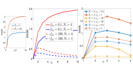
Figure 3: Left image: This figure compares the DASE levels between single-antenna and multi-antenna transmitters. The used parameters are as follows: ${f_{d}}_{1}=10,{f_{d}}_{2}=1,f_{c}=1000,{\rm PL}_{1}=.5,{\rm PL}_{2}=0,q_{\max}=20,M=1,{P_{p}}_{\max}={P_{d}}_{\max}={{P_{p}}_{2}}_{\max}={{P_{d}}_{2}}_{\max}=1,{\rm SNR}=0dB,N_{r}=10,\tau_{p}=10$. Middle image: DASE versus Doppler frequency. The used parameters are ${f_{d}}_{1}=0.1,{f_{d}}_{2}=100,f_{c}=1000,{\rm PL}_{1}=0,{\rm PL}_{2}=0,q_{\max}=10,M=1,{P_{p}}_{\max}={P_{d}}_{\max}={{P_{p}}_{2}}_{\max}={{P_{d}}_{2}}_{\max}=1,{\rm SNR}=0dB,N_{r}=10,\tau_{p}=4$. Right image: DASE versus the power ratio of the tagged user . The used parameters are ${f_{d}}_{1}=50,{f_{d}}_{2}=100,f_{c}=1000,{\rm PL}_{1}=1,{\rm PL}_{2}=0,q_{\max}=5,M=1,{{P_{p}}_{2}}_{\max}={{P_{d}}_{2}}_{\max}=1,P_{\rm tot}=5,N_{r}=20,\tau_{p}=5,\sigma^{2}_{p}=\sigma_{d}^{2}=7.94\times 10^{-5},{\sigma^{2}_{p}}_{2}=10^{-4}$.

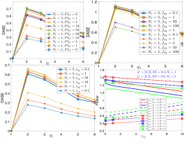
Figure 4: Top-left image: DASE versus the interference path loss. The used parameters are ${f_{d}}_{1}={f_{d}}_{2}=100,f_{c}=1000,{\rm PL}_{1}=1,q_{\max}=6,M_{\max}=1,{{P_{p}}_{1}}_{\max}={{P_{d}}_{1}}_{\max}={{P_{p}}_{2}}_{\max}={{P_{d}}_{2}}_{\max}=1,N_{r}=10,\tau_{p}=5,\sigma^{2}_{p}=\sigma_{d}^{2}=7.94\times 10^{-5},{\sigma^{2}_{p}}_{2}=10^{-4}$. Top-right image: DASE versus the interference maximum Doppler frequency . The used parameters are ${f_{d}}_{1}=100,f_{c}=1000,{\rm PL}_{1}=1,{\rm PL}_{2}=0,q_{\max}=6,M_{\max}=1,{{P_{p}}_{1}}_{\max}={{P_{d}}_{1}}_{\max}={{P_{p}}_{2}}_{\max}={{P_{d}}_{2}}_{\max}=1,N_{r}=10,\tau_{p}=5,\rho_{1}=0.9,\rho_{2}=0,\sigma^{2}_{p}=\sigma_{d}^{2}=7.94\times 10^{-5},{\sigma^{2}_{p}}_{2}=10^{-4}$. Bottom-left image: DASE versus the interference the power ratio of the interference. The used parameters are ${f_{d}}_{1}=100,f_{c}=1000,{\rm PL}_{1}=1,{\rm PL}_{2}=0,q_{\max}=6,M_{\max}=1,{{P_{p}}_{1}}_{\max}={{P_{d}}_{1}}_{\max}=1,N_{r}=10,\tau_{p}=5,\sigma^{2}_{p}=\sigma_{d}^{2}=7.94\times 10^{-5},{\sigma^{2}_{p}}_{2}=10^{-4}.$ Bottom-right image: Pilot and data powers versus the power ratio of the interference . The used parameters are ${f_{d}}_{1}={f_{d}}_{2}=100,f_{c}=1000,{\rm PL}_{1}=10,{\rm PL}_{2}=1,q_{\max}=6,M_{\max}=3,{P_{\rm tot}}_{1}={P_{\rm tot}}_{2}=2,N_{r}=10,\tau_{p}=10,\sigma^{2}_{p}=\sigma_{d}^{2}=7.94\times 10^{-5},{\sigma^{2}_{p}}_{2}=10^{-4}$.

V Conclusions

This work delved into the uplink communications of MIMO multi-user systems featuring multiple transmit and receive antennas, operating over fast-fading non-stationary wireless channels that undergo aging between consecutive pilot signals. A dedicated beamforming framework was developed to address spatial correlations among transmit antennas, complemented by a channel estimation process that capitalizes on the temporal correlations of the channel. Subsequently, a deterministic expression was introduced to approximate the average spectral efficiency in scenarios involving multi-frame data transmission. To enhance the performance further, an optimization framework was proposed to determine the optimal values for beamforming vectors, the number of frames, frame sizes, and power control, while satisfying some power constraints. Notably, our optimization approach exclusively leverages the knowledge of the temporal dynamics of the channel, eliminating the need for measurements or channel estimates. More importantly, optimal frame design and pilot spacing were demonstrated to be unaffected by the velocity of interference users and interference path loss. Furthermore, we showed that the impact of interference path loss and velocity diminishes as the number of transmit antennas increased. Simulation results robustly validated the effectiveness of our methodology, underscoring its profound influence on optimizing beamforming, pilot and data powers, frame sizes, and the number of frames across various practical scenarios.

Appendix A Proof of Proposition 1

At time $t$, the centered normalized channel can be described as follows:

$$\mathbf{h}^{\prime}(t)=\tfrac{1}{\sqrt{L(t)N}}\sum_{i=1}^{L(t)}{\rm e}^{j(2\pi f_{d}^{i}(t)t+\beta_{i})}\mathbf{a}_{R}(\theta^{i}_{\rm AoA})\otimes\mathbf{a}_{T}(\theta^{i}_{\rm AoD})$$ (36)

where

$$\mathbf{a}_{R}(\theta)=[1,{\rm e}^{j\tfrac{2\pi d_{R}\cos(\alpha-\theta)}{\lambda}},...,{\rm e}^{j\tfrac{2\pi d_{R}\cos(\alpha-\theta)(N_{r}-1)}{\lambda}}]^{\rm T}$$ (37)

and

$$\mathbf{a}_{T}(\theta)=[1,{\rm e}^{j\tfrac{2\pi d_{T}\cos(\alpha-\theta)}{\lambda}},...,{\rm e}^{j\tfrac{2\pi d_{T}\cos(\gamma(t)-\theta)(N_{t}-1)}{\lambda}}]^{\rm T}$$ (38)

are the array response vectors corresponding to the receiver and transmitter, respectively. $\beta_{i}$ is the phase of the $i$-th NLoS path. Now, we can proceed to obtain the correlation matrix between times $t_{1}$ and $t_{2}$ as follows:

$$\rho(t_{1},t_{2})=\mathds{E}[\mathbf{h}^{\prime}(t_{1})\mathbf{h}^{\prime}(t_{2})^{\rm H}]=\tfrac{1}{\sqrt{s(t_{1})s(t_{2})}N_{r}N_{t}}$$

$$=\tfrac{1}{\sqrt{s(t_{1})s(t_{2})}N_{r}N_{t}}\mathds{E}\Big{[}\sum_{i=1}^{\min(s(t_{1}),s(t_{2}))}{\rm e}^{j\Big{(}2\pi\big{(}f_{d}^{i}(t_{1})t_{1}-f_{d}^{i}(t_{2})t_{2}\big{)}\Big{)}}$$

$$\mathbf{a}_{R}(\theta_{\rm AoA}^{i}(t_{1}))\mathbf{a}_{R}^{\rm H}(\theta_{\rm AoA}^{i}(t_{2}))\otimes\mathbf{a}_{T}(\theta_{\rm AoD}^{i}(t_{1}))\mathbf{a}_{T}^{\rm H}(\theta_{\rm AoD}^{i}(t_{2}))\Big{]}$$ (39)

where in the second equality, we used the fact that the phases $\beta_{i}$s are independent and zero mean and also independent of AoAs and AoDs. When the number of scatterers goes to infinity, then by using central limit theorem, (A) can be approximated by the relation (1).

In the special case of Corollary 1 where the statistics of user and the environment do not change with time, then the parameters $\nu(t)=\nu,\gamma(t)=\gamma,\theta_{\rm AoA}(t)=\theta_{\rm AoA},\theta_{\rm AoD}(t)=\theta_{\rm AoD}$ are fixed. Define $\tau=t_{2}-t_{1}$ and $n_{R}=q-p,n_{T}=w-v$. When the AoA and AoD follow von Mises distribution with PDFs provided in (8), we can calculate the first and second terms in (1) as follows:

$$I_{2}=\mathds{E}\Big{[}{\rm e}^{j\tfrac{2\pi d_{R}}{\lambda}\big{[}p\cos(\alpha-\theta_{\rm AoA}(t_{1}))-q\cos(\alpha-\theta_{\rm AoA}(t_{2}))\big{]}}\Big{]}.$$ (40)

By exploiting the trigonometric property [36] and the definition of Bessel function of zero kind, the latter integral has a closed-form solution provided in (9). With the obtained integrals in (9), we can obtain the correlation elements for von Mises distribution as in $\rho(t_{1},t_{2},p,q,v,w)=I_{1}I_{2}.$ In the special case of Corollary 2 where $\kappa_{AoD}=\kappa_{AoA}=0$, we have a uniform distribution for AoD and AoA. In this simple case, the correlation becomes in the form of (11).

Appendix B Proof of Theorem 1

Based on the received measurements at data time slots, the BS employs the optimal MMSE receiver to estimate the transmitted data symbol of the tagged user at time slot $i$,i.e., $\widehat{{s}}(i)=\mathbf{g}^{\star}(i)\mathbf{y}_{\rm d}$. The expected energy of $\widehat{{s}}(i)$ conditioned on the channel estimates at time slots $i$ and $i_{p}$ is given by:

$$\mathds{E}_{{s},\mathbf{n}_{d},\mathbf{h}(i)|\bm{\zeta}(i)}|{\widehat{{s}}(i)}|^{2}=\langle\mathbf{g}^{\rm H}\mathbf{g},\mathds{E}\mathbf{y}_{\rm d}\mathbf{y}_{\rm d}^{\rm H}|\bm{\zeta}(i)\rangle.$$ (41)

By using the closed-form expression for $\mathds{E}\mathbf{y}_{\rm d}\mathbf{y}_{\rm d}^{\rm H}|\bm{\zeta}(i)$ which is provided in Equation 18 in Appendix I of the supplementary material, and replacing in the above formulation, it follows that:

$$\mathds{E}_{\mathbf{n}_{d},\mathbf{h}(i)|\bm{\zeta}(i)}|\widehat{s}(i)|^{2}=\sum_{k=1}^{K}\alpha_{k}^{2}\langle\mathbf{g}^{\rm H}\mathbf{g},\mathcal{A}_{k}(\mathbf{D}_{k})\rangle+\sigma^{2}_{d}\|\mathbf{g}\|_{2}^{2}$$

$$=\sum_{k=1}^{K}\alpha_{k}^{2}\langle\mathcal{A}_{k}^{\rm Adj}(\mathbf{g}^{\rm H}\mathbf{g}),\mathbf{D}_{k}\rangle+\sigma^{2}_{d}\|\mathbf{g}\|_{2}^{2},$$ (42)

where $\mathbf{D}_{k}=\mathbf{Q}_{k}+\mathbf{z}_{k}\mathbf{z}_{k}^{\rm H}$ , $\mathbf{z}_{k}=\bm{\Psi}_{k}\widetilde{\bm{\zeta}}_{k}(i)$ and $\mathcal{A}^{\rm Adj}(\cdot)$ is the adjoint operator which can be obtained as stated in the following lemma and is proved in Appendix V of the supplementary material.

Lemma 2.

The ad-joint of $\mathcal{A}_{k}(\cdot)$ is obtained as:

$$\mathcal{A}^{Adj}(\mathbf{Y})=\mathbf{C}_{\mathbf{x}}\otimes\mathbf{Y}.$$ (43)

Now, by characterizing the adjoint operator, we can rewrite (B) as follows:

$$\mathds{E}_{\mathbf{n}_{d},\mathbf{h}(i)|\bm{\zeta}(i)}|\widehat{s}|^{2}=\alpha^{2}\left\langle\mathbf{z}_{1}\mathbf{z}_{1}^{\rm H},\mathbf{C}_{\mathbf{x}}\otimes\mathbf{g}^{\rm H}\mathbf{g}\right\rangle+$$

(44)

By having the expected energy of estimated data symbols, we can now form the instantaneous SINR of the symbol estimate in slot $i$ of frame $m$ corresponding to the tagged user as follows:

(45)

By having the definition of $\mathbf{F}_{1}$ in Theorem 1 and (B) in mind, the instantaneous SINR can be rewritten as

$$\gamma(\mathbf{q},i,\zeta(i))=\tfrac{\left\langle\mathbf{g}^{\rm H}\mathbf{g},\mathbf{F}-\mathbf{F}_{1}\right\rangle}{\left\langle\mathbf{g}^{\rm H}\mathbf{g},\mathbf{F}_{1}\right\rangle}.$$ (46)

It then follows that based on (19), $\mathbf{g}^{\rm H}\mathbf{g}$ can be stated as:

$$\mathbf{g}^{\rm H}\mathbf{g}=\alpha_{1}^{2}P_{\rm d}\mathbf{F}^{-1}\mathbf{J}_{1}\mathbf{w}\mathbf{w}^{\rm H}\mathbf{J}_{1}^{\rm H}\mathbf{F}^{-1}.$$ (47)

Moreover, the following proposition will be required later:

Proposition 4.

For any operator $\mathcal{A}(\cdot):\mathbb{C}^{N_{t}N_{r}\times N_{t}N_{r}}\rightarrow\mathbb{C}^{N_{r}\times N_{r}}$, the following relationship holds:

$$\mathcal{A}(\mathbf{z}\mathbf{z}^{\rm H})=\mathbf{J}\mathbf{C}_{\mathbf{x}}\mathbf{J}^{\rm H}.$$ (48)

Proof. See Appendix IV of the supplementary material.

By incorporating (48) and (47) into (46), we reach to the following relation:

$$\gamma(\mathbf{q},i,\zeta(i))=\tfrac{\alpha_{1}^{2}P_{\rm d}\left\langle\mathbf{F}^{-1}\mathbf{J}\mathbf{w}\mathbf{w}^{\rm H}\mathbf{J}^{\rm H}\mathbf{F}^{-1},\alpha^{2}\mathbf{J}\mathbf{C}_{\mathbf{x}}\mathbf{J}^{\rm H}\right\rangle}{\alpha_{1}^{2}P_{1}\left\langle\mathbf{F}^{-1}\mathbf{J}\mathbf{w}\mathbf{w}^{\rm H}\mathbf{J}^{\rm H}\mathbf{F}^{-1},\mathbf{F}-\alpha^{2}\mathbf{J}\mathbf{w}\mathbf{w}^{\rm H}\mathbf{J}^{\rm H}\right\rangle}=$$

$$\tfrac{\alpha_{1}^{2}P_{\rm d}\left\langle\mathbf{F}^{-1}\mathbf{J}\mathbf{w}\mathbf{w}^{\rm H}\mathbf{J}^{\rm H}\mathbf{F}^{-1},\mathbf{J}\mathbf{C}_{\mathbf{x}}\mathbf{J}^{\rm H}\right\rangle}{\left\langle\mathbf{F}^{-1}\mathbf{J}\mathbf{w}\mathbf{w}^{\rm H}\mathbf{J}^{\rm H}\mathbf{F}^{-1},F\right\rangle-\alpha_{1}^{2}\left\langle\mathbf{F}^{-1}\mathbf{J}\mathbf{w}\mathbf{w}^{\rm H}\mathbf{J}^{\rm H}\mathbf{F}^{-1},\mathbf{J}\mathbf{C}_{\mathbf{x}}\mathbf{J}^{\rm H}\right\rangle}.$$ (49)

When a single symbol is transmitted through multiple antennas at the user side, the covariance matrix satisfy $\mathbf{C}_{\mathbf{x}}=P_{\rm d}\mathbf{w}\mathbf{w}^{\rm H}$ where $\|\mathbf{w}\|_{2}=1$. By using the rotational invariance property of the Frobinous inner product in the numerator of (B), we can rewrite the numerator of (B) as follows

(50)

Also, the first term in the denominator of (B) is simplified as

$${\rm tr}(\mathbf{F}^{-1}\mathbf{J}\mathbf{w}\mathbf{w}^{\rm H}\mathbf{J}^{\rm H}\mathbf{F}^{-1}\mathbf{F})=\mathbf{w}^{\rm H}\mathbf{J}^{\rm H}\mathbf{F}^{-1}\mathbf{J}\mathbf{w}.$$ (51)

By having (50) and (51), the SINR expression in (B) simplifies to

$$\gamma(\mathbf{q},i,\zeta(i))=\tfrac{\alpha^{2}P_{\rm d}\mathbf{w}^{\rm H}\mathbf{J}^{\rm H}\mathbf{F}^{-1}\mathbf{J}\mathbf{w}}{1-\alpha^{2}P_{\rm d}\mathbf{w}^{\rm H}\mathbf{J}^{\rm H}\mathbf{F}^{-1}\mathbf{J}\mathbf{w}}.$$ (52)

Now, we can use the following lemma whose proof is provided in Appendix III of the supplementary material.

Lemma 3.

Let $\mathbf{A}\in\mathbb{C}^{N_{r}\times N_{r}}$ be an invertible matrix and $\beta$ is a scalar. For any $\mathbf{z}\in\mathbb{C}^{N_{r}\times 1}$, it holds that

$$\tfrac{\mathbf{z}^{\rm H}\mathbf{A}\mathbf{z}}{\beta-\mathbf{z}^{\rm H}\mathbf{A}\mathbf{z}}=\mathbf{z}^{\rm H}\left(\beta\mathbf{A}^{-1}-\mathbf{z}\mathbf{z}^{\rm H}\right)^{-1}\mathbf{z}.$$ (53)

By replacing $\mathbf{z}=\mathbf{J}\mathbf{w}$ and $\mathbf{A}=\mathbf{F}^{-1}$ in Lemma 3 and using the definition of $\mathbf{F}_{1}$ in Theorem 1 and Proposition 4, we have

$$\gamma(\mathbf{q},i,\zeta(i))=\alpha^{2}P_{\rm d}\mathbf{w}^{\rm H}\mathbf{J}^{\rm H}\left(\mathbf{F}-\alpha^{2}\mathbf{J}\mathbf{w}\mathbf{w}^{\rm H}\mathbf{J}^{\rm H}\right)^{-1}\mathbf{J}\mathbf{w}$$

$$=\alpha^{2}P_{\rm d}\mathbf{w}^{\rm H}\mathbf{J}^{\rm H}\mathbf{F}_{1}^{-1}\mathbf{J}\mathbf{w}=\alpha^{2}P_{\rm d}\left\langle\mathbf{J}\mathbf{w}\mathbf{w}^{\rm H}\mathbf{J}^{\rm H},\mathbf{F}_{1}^{-1}\right\rangle=$$

$$\alpha^{2}\left\langle\mathcal{A}(\mathbf{z}\mathbf{z}^{\rm H}),\mathbf{F}_{1}^{-1}\right\rangle=\alpha^{2}\left\langle\mathbf{z}\mathbf{z}^{\rm H},\mathbf{C}_{\mathbf{x}}\otimes\mathbf{F}_{1}^{-1}\right\rangle=$$

$$\alpha^{2}\mathbf{z}^{\rm H}\left(\mathbf{C}_{\mathbf{x}}\otimes\mathbf{F}_{1}^{-1}\right)\mathbf{z},$$ (54)

which proves the result.

Appendix C Proof of Theorem 2

Define the expectation of SE and SINR, by

$$\overline{\textup{SE}}(\mathbf{q},i)\mathbin{\setstackgap{S}{0pt}\stackMath\Shortstack{\smalltriangleup{\\ }=}}\mathds{E}\left[\textup{SE}(\mathbf{q},i,\bm{\zeta}(i))\right],\overline{\gamma}(\mathbf{q},i)\mathbin{\setstackgap{S}{0pt}\stackMath\Shortstack{\smalltriangleup{\\ }=}}\mathds{E}\left[\gamma(\mathbf{q},i,\bm{\zeta}(i))\right].$$ (55)

The aim is to find an equivalent deterministic expression denoted by ${\rm SE}^{\circ}(\mathbf{q},i)\mathbin{\setstackgap{S}{0pt}\stackMath\Shortstack{\smalltriangleup\\ =}}\log(1+\gamma^{\circ}(\mathbf{q},i))$ that approximates the average SE $\overline{\textup{SE}}(\mathbf{q},i)$ at time slot $i$. Here, $\gamma^{\circ}(\mathbf{q},i)$ is a deterministic equivalent expression for the SINR to be defined later. First, we claim that $\overline{\textup{SE}}(\mathbf{q},i)$ is close to the equivalent deterministic SE expression as long as $\overline{\gamma}(\mathbf{q},i)$ is sufficiently close to $\gamma^{\circ}(\mathbf{q},i)$ as is shown in the following error bound for Jensen’s inequality [37]:

$$\tfrac{1}{N_{r}}\left|\overline{\textup{SE}}(\mathbf{q},i)-\log(1+{\gamma}^{\circ}(\mathbf{q},i))\right|\leq\tfrac{c^{\prime}}{N_{r}}\left[\Big{|}\overline{\gamma}(\mathbf{q},i)-{\gamma}^{\circ}(\mathbf{q},i)\Big{|}\right],$$ (56)

where $c^{\prime}$ is some constant term independent of the frame parameters. The latter bound stems from Jensen’s inequality error estimate bounds that provides an upper-bound for the error of passing the expectation operator from a concave function. In what follows, we show that the instantaneous SINR $\gamma(\mathbf{q},i,\bm{\zeta}(i))$ concentrates around its expectation $\overline{\gamma}$ and then $\overline{\gamma}$ is well approximated by the SINR expression ${\gamma}^{\circ}(\mathbf{q},i)$.

Define $\mathbf{B}=\sum_{k=2}^{K}\alpha_{k}^{2}\mathcal{A}_{k}(\mathbf{z}_{k}\mathbf{z}_{k}^{\rm H})+\bm{\Theta}$, we can write $\mathbf{F}_{1}$ in Theorem 1 as $\mathbf{F}_{1}=\mathbf{B}+\bm{\Theta}+\rho_{\rm d}\mathbf{I}_{N_{r}}$.

$$\tfrac{\overline{\gamma}(\mathbf{q},i)}{N_{r}}=\tfrac{1}{N_{r}}\alpha_{1}^{2}\left\langle\mathbf{C}_{\mathbf{z}_{1}},\mathbf{C}_{\mathbf{x}_{1}}\otimes\mathds{E}[{\mathbf{F}_{1}}^{-1}]\right\rangle\stackrel{{\scriptstyle N_{r}\rightarrow\infty}}{{=}}$$

$$\tfrac{1}{N_{r}}\alpha_{1}^{2}\left\langle\mathbf{C}_{\mathbf{z}_{1}},\mathbf{C}_{\mathbf{x}_{1}}\otimes\bm{\Xi}^{-1}\right\rangle\mathbin{\setstackgap{S}{0pt}\stackMath\Shortstack{\smalltriangleup{\\ }=}}\tfrac{{\gamma}^{\circ}(\mathbf{q},i)}{N_{r}}$$ (57)

where $\bm{\Xi}\mathbin{\setstackgap{S}{0pt}\stackMath\Shortstack{\smalltriangleup\\ =}}\mathbf{\Gamma}+\bm{\Theta}+\rho_{\rm d}\mathbf{I}_{N_{r}}$ and $\mathbf{\Gamma}$ is a matrix depending on the Stieltjes transform corresponding to the empirical distribution of $\mathbf{B}$ and is determined later.

The approximation error in (C) is defined as the difference between $\gamma(\mathbf{q},i)$ and $\gamma^{\circ}(\mathbf{q},i)$ given by:

$$e_{N}=\tfrac{\alpha_{1}^{2}}{N_{r}}\left\langle\mathcal{A}_{1}(\mathbf{C}_{\mathbf{z}_{1}}),(\mathbf{B}+\rho_{\rm d}\mathbf{I}_{N_{r}})^{-1}\right\rangle-\tfrac{\alpha_{1}^{2}}{N_{r}}\left\langle\mathcal{A}_{1}(\mathbf{C}_{\mathbf{z}_{1}}),\bm{\Xi}^{-1}\right\rangle.$$ (58)

The aim is to show that $e_{N}\xrightarrow[]{N_{r}\rightarrow\infty}0$ with high probability. First, we state the resolvent matrix identity between two matrices i.e.

$$\mathbf{U}^{-1}-\mathbf{V}^{-1}=\mathbf{V}^{-1}(\mathbf{V}-\mathbf{U})\mathbf{U}^{-1},\forall\mathbf{U},\mathbf{V}$$ (59)

to have

(60)

We can proceed with (60) as follows:

$$(\mathbf{B}+\rho_{\rm d}\mathbf{I}_{N_{r}})^{-1}-\bm{\Xi}^{-1}=\bm{\Xi}^{-1}\mathbf{\Gamma}(\mathbf{B}+\rho_{\rm d}\mathbf{I}_{N_{r}})^{-1}$$

$$-\sum_{k=2}^{K}\alpha_{k}^{2}\bm{\Xi}^{-1}\mathcal{A}_{k}(\mathbf{z}_{k}^{\prime}{\mathbf{z}_{k}^{\prime}}^{\rm H})(\mathbf{B}+\rho_{\rm d}\mathbf{I}_{N_{r}})^{-1}.$$ (61)

Now, the residual $e_{N}$ in (58) becomes as

$$e_{N}=\tfrac{\alpha_{1}^{2}}{N_{r}}\left\langle\mathcal{A}_{1}(\mathbf{C}_{\mathbf{z}_{1}}),\bm{\Xi}^{-1}\mathbf{\Gamma}(\mathbf{B}+\rho_{\rm d}\mathbf{I}_{N_{r}})^{-1}\right\rangle-$$

$$\tfrac{\alpha_{1}^{2}}{N_{r}}\sum_{k=2}^{K}\alpha_{k}^{2}\left\langle\mathcal{A}_{1}(\mathbf{C}_{\mathbf{z}_{1}}),\bm{\Xi}^{-1}\mathcal{A}_{k}(\mathbf{z}_{k}{\mathbf{z}_{k}}^{\rm H})(\mathbf{B}+\rho_{\rm d}\mathbf{I}_{N_{r}})^{-1}\right\rangle.$$ (62)

Due to the relation 48, it follows that

$$\langle\mathcal{A}_{k}(\mathbf{z}_{k}{\mathbf{z}_{k}}^{\rm H}),\bm{\Xi}^{-1}\mathcal{A}_{1}(\mathbf{C}_{\mathbf{z}_{1}})(\mathbf{B}+\rho_{\rm d}\mathbf{I}_{N_{r}})^{-1}\rangle$$

$$\langle\mathbf{J}_{k}\mathbf{C}_{\mathbf{x}_{k}}{\mathbf{J}_{k}}^{\rm H},\bm{\Xi}^{-1}\mathcal{A}_{1}(\mathbf{C}_{\mathbf{z}_{1}})(\mathbf{B}+\rho_{\rm d}\mathbf{I}_{N_{r}})^{-1}\rangle=$$

$$P_{d_{k}}\mathbf{w}_{k}^{\rm H}{\mathbf{J}_{k}}^{\rm H}(\mathbf{B}+\rho_{\rm d}\mathbf{I}_{N_{r}})^{-1}\mathcal{A}_{1}(\mathbf{C}_{\mathbf{z}_{1}})\bm{\Xi}^{-1}\mathbf{J}_{k}\mathbf{w}_{k},$$ (63)

where in the last step, we used the definition of the covariance matrix $\mathbf{C}_{\mathbf{x}_{k}}=P_{{\rm d},k}\mathbf{w}_{k}\mathbf{w}_{k}^{\rm H}$ and trace rotational invariance property. Now, by using [38, Equation 2.2], it follows that

$$\mathbf{w}_{k}^{\rm H}{\mathbf{J}_{k}}^{\rm H}(\mathbf{B}+\rho_{\rm d}\mathbf{I}_{N_{r}})^{-1}=\tfrac{\mathbf{w}_{k}^{\rm H}{\mathbf{J}_{k}}^{\rm H}(\mathbf{B}_{(k)}+\rho_{\rm d}\mathbf{I}_{N_{r}})^{-1}}{1+\alpha_{k}^{2}P_{{\rm d},k}\mathbf{w}_{k}^{\rm H}{\mathbf{J}_{k}}^{\rm H}(\mathbf{B}_{(k)}+\rho_{\rm d}\mathbf{I}_{N_{r}})^{-1}\mathbf{J}_{k}\mathbf{w}_{k}},$$ (64)

in which $\mathbf{B}_{(k)}\mathbin{\setstackgap{S}{0pt}\stackMath\Shortstack{\smalltriangleup\\ =}}\mathbf{B}-\alpha_{k}^{2}\mathbf{J}_{k}\mathbf{C}_{\mathbf{x}_{k}}{\mathbf{J}_{k}}^{\rm H}$. We also have:

(65)

By incorporating (64) and (65) into (C), the approximation error reads as:

$$e_{N}=\tfrac{\alpha_{1}^{2}}{N_{r}}\sum_{k=2}^{K}\alpha_{k}^{2}\tfrac{{\mathbf{z}_{k}}^{\rm H}\left(\mathbf{C}_{\mathbf{x}_{k}}\otimes(\mathbf{B}_{(k)}+\rho_{\rm d}\mathbf{I}_{N_{r}})^{-1}\mathcal{A}_{1}(\mathbf{C}_{\mathbf{z}_{1}})\bm{\Xi}^{-1}\right)\mathbf{z}_{k}}{1+\alpha_{k}^{2}{\mathbf{z}_{k}}^{H}\mathbf{C}_{\mathbf{x}_{k}}\otimes(\mathbf{B}_{(k)}+\rho_{\rm d}\mathbf{I}_{N_{r}})^{-1}\mathbf{z}_{k}}-$$

$$\tfrac{\alpha_{1}^{2}}{N_{r}}\left\langle\mathcal{A}_{1}(\mathbf{C}_{\mathbf{z}_{1}}),\bm{\Xi}^{-1}\mathbf{\Gamma}(\mathbf{B}+\rho_{\rm d}\mathbf{I}_{N_{r}})^{-1}\right\rangle.$$ (66)

In what follows, we will prove that by the choice of $\mathbf{\Gamma}$ as

$$\mathbf{\Gamma}=\sum_{k=2}^{K}\tfrac{\alpha_{k}^{2}\mathcal{A}_{k}(\mathbf{C}_{\mathbf{z}_{k}})}{1+\alpha_{k}^{2}N_{r}m_{{\mathbf{C}_{\mathbf{z}_{k}},\mathbf{B}}}(\rho_{\rm d})},$$ (67)

where $m_{{\mathbf{C}_{\mathbf{z}_{k}},\mathbf{B}}}(\rho_{\rm d})\mathbin{\setstackgap{S}{0pt}\stackMath\Shortstack{\smalltriangleup\\ =}}\tfrac{1}{N_{r}}\langle\mathbf{C}_{\mathbf{z}_{k}},\mathbf{C}_{\mathbf{x}_{k}}\otimes(\mathbf{B}+\rho_{\rm d}\mathbf{I}_{N_{r}})^{-1}\rangle$. The residual $e_{N}$ goes to zero as $N_{r}$ goes to infinity. To see this, first, we replace this specific choice of $\mathbf{\Gamma}$ into (C) to form $e_{N}$ as follows:

$$e_{N}=\tfrac{\alpha_{1}^{2}}{N_{r}}\sum_{k=2}^{K}\alpha_{k}^{2}\tfrac{{\mathbf{z}_{k}}^{H}\left(\mathbf{C}_{\mathbf{x}_{k}}\otimes(\mathbf{B}_{(k)}+\rho_{\rm d}\mathbf{I}_{N_{r}})^{-1}\mathcal{A}_{1}(\mathbf{C}_{\mathbf{z}_{1}})\bm{\Xi}^{-1}\right){\mathbf{z}_{k}}}{1+\alpha_{k}^{2}{\mathbf{z}_{k}}^{H}\mathbf{C}_{\mathbf{x}_{k}}\otimes(\mathbf{B}_{(k)}+\rho_{\rm d}\mathbf{I}_{N_{r}})^{-1}{\mathbf{z}_{k}}}$$

(68)

where

$$d_{k}=\tfrac{\alpha_{1}^{2}}{N_{r}}\tfrac{{\mathbf{z}_{k}}^{H}\left(\mathbf{C}_{\mathbf{x}_{k}}\otimes(\mathbf{B}_{(k)}+\rho_{\rm d}\mathbf{I}_{N_{r}})^{-1}\mathcal{A}_{1}(\mathbf{C}_{\mathbf{z}_{1}}){{\bm{\Xi}}^{\prime}}^{-1}\right)\mathbf{z}_{k}}{1+\alpha_{k}^{2}{\mathbf{z}_{k}}^{H}\mathbf{C}_{\mathbf{x}_{k}}\otimes(\mathbf{B}_{(k)}+\rho_{\rm d}\mathbf{I}_{N_{r}})^{-1}\mathbf{z}_{k}}$$

$$-\tfrac{\alpha_{1}^{2}}{N_{r}}\tfrac{\left\langle\mathcal{A}_{k}(\mathbf{C}_{\mathbf{z}_{k}}),{{\bm{\Xi}}^{\prime}}^{-1}\mathcal{A}_{1}(\mathbf{C}_{\mathbf{z}_{1}})(\mathbf{B}+\rho_{\rm d}\mathbf{I}_{N_{r}})^{-1}\right\rangle}{1+\alpha_{k}^{2}N_{r}m_{{\mathbf{C}_{\mathbf{z}_{k}},\mathbf{B}}}(\rho_{\rm d})},$$ (69)

where $\bm{\Xi}^{\prime}\mathbin{\setstackgap{S}{0pt}\stackMath\Shortstack{\smalltriangleup\\ =}}\tfrac{1}{K-1}\bm{\Xi}$. Define

$${\bm{\Xi}^{\prime}}_{(k)}\mathbin{\setstackgap{S}{0pt}\stackMath\Shortstack{\smalltriangleup{\\ }=}}\frac{1}{K-1}\sum_{k=2}^{K}\tfrac{\alpha_{k}^{2}\mathcal{A}_{k}(\mathbf{C}_{\mathbf{z}_{k}})}{1+\alpha_{k}^{2}N_{r}m_{{\mathbf{C}_{\mathbf{z}_{k}},\mathbf{B}_{(k)}}}(\rho_{\rm d})}+\tfrac{\bm{\Theta}}{K-1}+\tfrac{\rho_{\rm d}}{K-1}\mathbf{I}_{N_{r}}.$$ (70)

$d_{k}$ in the relation (C) can be stated as the sum of $4$ terms as below:

$$d_{k}=d_{k}^{(1)}+d_{k}^{(2)}+d_{k}^{(3)}+d_{k}^{(4)},$$ (71)

where

$$d_{k}^{(1)}=\tfrac{\alpha_{1}^{2}}{N_{r}}\tfrac{\mathbf{z}_{k}^{H}\left(\mathbf{C}_{\mathbf{x}_{k}}\otimes(\mathbf{B}_{(k)}+\rho_{\rm d}\mathbf{I}_{N_{r}})^{-1}\mathcal{A}_{1}(\mathbf{C}_{\mathbf{z}_{1}}){\bm{\Xi}^{\prime}}^{-1}\right)\mathbf{z}_{k}}{1+\alpha_{k}^{2}{\mathbf{z}_{k}}^{H}\mathbf{C}_{\mathbf{x}_{k}}\otimes(\mathbf{B}_{(k)}+\rho_{\rm d}\mathbf{I}_{N_{r}})^{-1}\mathbf{z}_{k}}-\tfrac{\alpha_{1}^{2}}{N_{r}},$$

$$\tfrac{\mathbf{z}_{k}^{H}\left(\mathbf{C}_{\mathbf{x}_{k}}\otimes(\mathbf{B}_{(k)}+\rho_{\rm d}\mathbf{I}_{N_{r}})^{-1}\mathcal{A}_{1}(\mathbf{C}_{\mathbf{z}_{1}}){\bm{\Xi}^{\prime}}_{(k)}^{-1}\right)\mathbf{z}_{k}}{1+\alpha_{k}^{2}{\mathbf{z}_{k}}^{H}\mathbf{C}_{\mathbf{x}_{k}}\otimes(\mathbf{B}_{(k)}+\rho_{\rm d}\mathbf{I}_{N_{r}})^{-1}\mathbf{z}_{k}},$$ (72)

$$d_{k}^{(2)}=\tfrac{\alpha_{1}^{2}}{N_{r}}\tfrac{\mathbf{z}_{k}^{H}\left(\mathbf{C}_{\mathbf{x}_{k}}\otimes(\mathbf{B}_{(k)}+\rho_{\rm d}\mathbf{I}_{N_{r}})^{-1}\mathcal{A}_{1}(\mathbf{C}_{\mathbf{z}_{1}}){\bm{\Xi}^{\prime}}_{(k)}^{-1}\right)\mathbf{z}_{k}}{1+\alpha_{k}^{2}{\mathbf{z}_{k}}^{H}\mathbf{C}_{\mathbf{x}_{k}}\otimes(\mathbf{B}_{(k)}+\rho_{\rm d}\mathbf{I}_{N_{r}})^{-1}\mathbf{z}_{k}}-$$

$$\tfrac{\alpha_{1}^{2}}{N_{r}}\tfrac{\langle\mathbf{C}_{\mathbf{z}_{k}},{\bm{\Xi}^{\prime}}_{(k)}^{-1}\mathcal{A}_{1}(\mathbf{C}_{\mathbf{z}_{1}})\mathbf{C}_{\mathbf{x}_{k}}\otimes(\mathbf{B}_{(k)}+\rho_{\rm d}\mathbf{I}_{N_{r}})^{-1}\rangle}{1+\alpha_{k}^{2}{\mathbf{z}_{k}}^{H}\mathbf{C}_{\mathbf{x}_{k}}\otimes(\mathbf{B}_{(k)}+\rho_{\rm d}\mathbf{I}_{N_{r}})^{-1}\mathbf{z}_{k}},$$ (73)

$$d_{k}^{(3)}=\tfrac{\alpha_{1}^{2}}{N_{r}}\tfrac{\langle\mathbf{C}_{\mathbf{z}_{k}},\mathbf{C}_{\mathbf{x}_{k}}\otimes{\bm{\Xi}^{\prime}}_{(k)}^{-1}\mathcal{A}_{1}(\mathbf{C}_{\mathbf{z}_{1}})(\mathbf{B}_{(k)}+\rho_{\rm d}\mathbf{I}_{N_{r}})^{-1}\rangle}{1+\alpha_{k}^{2}{\mathbf{z}_{k}}^{H}\mathbf{C}_{\mathbf{x}_{k}}\otimes(\mathbf{B}_{(k)}+\rho_{\rm d}\mathbf{I}_{N_{r}})^{-1}\mathbf{z}_{k}}-$$

$$\tfrac{\alpha_{1}^{2}}{N_{r}}\tfrac{\langle\mathbf{C}_{\mathbf{z}_{k}},\mathbf{C}_{\mathbf{x}_{k}}\otimes{\bm{\Xi}^{\prime}}^{-1}\mathcal{A}_{1}(\mathbf{C}_{\mathbf{z}_{1}})(\mathbf{B}+\rho_{\rm d}\mathbf{I}_{N_{r}})^{-1}\rangle}{1+\alpha_{k}^{2}{\mathbf{z}_{k}}^{H}\mathbf{C}_{\mathbf{x}_{k}}\otimes(\mathbf{B}_{(k)}+\rho_{\rm d}\mathbf{I}_{N_{r}})^{-1}\mathbf{z}_{k}},$$ (74)

$$d_{k}^{(4)}=\tfrac{\alpha_{1}^{2}}{N_{r}}\tfrac{\langle\mathbf{C}_{\mathbf{z}_{k}},\mathbf{C}_{\mathbf{x}_{k}}\otimes{\bm{\Xi}^{\prime}}^{-1}\mathcal{A}_{1}(\mathbf{C}_{\mathbf{z}_{1}})(\mathbf{B}+\rho_{\rm d}\mathbf{I}_{N_{r}})^{-1}\rangle}{1+\alpha_{k}^{2}{\mathbf{z}_{k}}^{H}\mathbf{C}_{\mathbf{x}_{k}}\otimes(\mathbf{B}+\rho_{\rm d}\mathbf{I}_{N_{r}})^{-1}\mathbf{z}_{k}}-$$

$$\tfrac{\alpha_{1}^{2}}{N_{r}}\tfrac{\langle\mathbf{C}_{\mathbf{z}_{k}},\mathbf{C}_{\mathbf{x}_{k}}\otimes{\bm{\Xi}^{\prime}}^{-1}\mathcal{A}_{1}(\mathbf{C}_{\mathbf{z}_{1}})(\mathbf{B}+\rho_{\rm d}\mathbf{I}_{N_{r}})^{-1}\rangle}{1+\alpha_{k}^{2}Nm_{{\mathbf{C}_{\mathbf{z}_{k}},\mathbf{B}_{(k)}}}(\rho_{\rm d})}.$$ (75)

To bound $d_{k}^{(1)}$, we use Lemma 4 whose proof is given in Appendix III of the supplementary material.

Lemma 4.

Let $\mathbf{J}\in\mathbb{C}^{N_{r}\times N_{t}}$, $\mathbf{B}$ be a Hermitian non-negative definite matrix and $\mathbf{C}$ is of size $N_{t}\times N_{t}$. Then for $t>0$ and $\rho_{\rm d}>0$, we have: $\left|\tfrac{1}{1+t\langle\mathbf{J}\mathbf{C}\mathbf{J}^{H},\left(\mathbf{B}+\rho_{\rm d}\mathbf{I}\right)^{-1}\rangle}\right|\leq 1$.

Proof. See Appendix III of the supplementary material.

It then follows that

$$\scalebox{0.9}{$|d_{k}^{(1)}|\leq\tfrac{\alpha_{1}^{2}P_{d,k}}{\alpha_{k}^{2}N_{r}N_{t}}\|\mathbf{z}_{k}\|_{2}^{2}\|(\mathbf{B}_{(k)}+\rho_{\rm d}\mathbf{I}_{N_{r}})^{-1}\|\|{\bm{\Xi}^{\prime}}^{-1}-{\bm{\Xi}^{\prime}}_{(k)}^{-1}\|\|\mathcal{A}_{1}(\mathbf{C}_{\mathbf{z}_{1}})\|$},$$ (76)

where we used Lemma 4. $(\mathbf{B}_{(k)}+\rho_{\rm d}\mathbf{I}_{N_{r}})^{-1}$ is the Stieltjes transform of a finite measure in $\mathbb{C}^{-}$, so by [39, Theorem 3.2], we have

$$\|\left(\mathbf{B}_{(k)}+\rho_{\rm d}\mathbf{I}_{N_{r}}\right)^{-1}\|\leq\tfrac{1}{|\rho_{\rm d}|}$$ (77)

To bound $\|{\bm{\Xi}^{\prime}}^{-1}-{\bm{\Xi}^{\prime}}_{(k)}^{-1}\|$, we can use the resolvent matrix identity (59) which leads to

$$\|{\bm{\Xi}^{\prime}}^{-1}-{\bm{\Xi}^{\prime}}_{(k)}^{-1}\|\leq\|{\bm{\Xi}^{\prime}}_{(k)}^{-1}\|\|{\bm{\Xi}^{\prime}}_{(k)}-{\bm{\Xi}^{\prime}}\|\|{\bm{\Xi}^{\prime}}^{-1}\|.$$ (78)

By [40, Lemma 8], we have that $\|{\bm{\Xi}^{\prime}}_{(k)}^{-1}\|$ and $\|{\bm{\Xi}^{\prime}}^{-1}\|$ are less than $\tfrac{1}{|\rho_{\rm d}|}$. Also, it follows that

$$\|{\bm{\Xi}^{\prime}}_{(k)}-{\bm{\Xi}^{\prime}}\|\leq\tfrac{\mu_{k}^{\prime}}{K-1}$$

$$\sum_{k=2}^{K}\alpha_{k}^{4}N_{r}\tfrac{|m_{\mathbf{C}_{\mathbf{z}_{k}},\mathbf{B}_{(k)}}(\rho_{\rm d})-m_{\mathbf{C}_{\mathbf{z}_{k}},\mathbf{B}}(\rho_{\rm d})|}{(1+\alpha_{k}^{2}N_{r}m_{\mathbf{C}_{\mathbf{z}_{k}},\mathbf{B}_{(k)}}(\rho_{\rm d}))(1+\alpha_{k}^{2}N_{r}m_{\mathbf{C}_{\mathbf{z}_{k}},\mathbf{B}}(\rho_{\rm d}))}\leq\tfrac{{\mu_{k}^{\prime}}^{4}}{|\rho_{\rm d}|},$$ (79)

where we used [41, Lemma 2.1], and

$$\|\mathcal{A}_{k}(\mathbf{C}_{\mathbf{z}_{k}})\|=\sup_{\begin{subarray}{c}\mathbf{x}\neq\mathbf{0}\\ \mathbf{y}\neq\mathbf{0}\end{subarray}}\tfrac{\langle\mathcal{A}_{k}(\mathbf{C}_{\mathbf{z}_{k}})\mathbf{y},\mathbf{x}\rangle}{\|\mathbf{x}\|_{2}\|\mathbf{y}\|_{2}}=\sup_{\begin{subarray}{c}\mathbf{x}\neq\mathbf{0}\\ \mathbf{y}\neq\mathbf{0}\end{subarray}}\tfrac{\langle\mathcal{A}_{k}(\mathbf{C}_{\mathbf{z}_{k}}),\mathbf{x}\mathbf{y}^{H}\rangle}{\|\mathbf{x}\|_{2}\|\mathbf{y}\|_{2}}$$

$$=\sup_{\begin{subarray}{c}\mathbf{x}\neq\mathbf{0}\\ \mathbf{y}\neq\mathbf{0}\end{subarray}}\tfrac{\langle\mathbf{C}_{\mathbf{z}_{k}},\mathbf{x}\mathbf{y}^{H}\otimes\mathbf{C}_{\mathbf{x}_{k}}\rangle}{\|\mathbf{x}\|_{2}\|\mathbf{y}\|_{2}}\leq{\rm tr}(\mathbf{C}_{\mathbf{z}_{k}})\|\mathbf{C}_{\mathbf{x}_{k}}\|\leq\tfrac{\Omega_{1}^{2}\Omega_{2}L_{k}}{N}\tfrac{{P_{d}}_{k}}{N_{t}}\mathbin{\setstackgap{S}{0pt}\stackMath\Shortstack{\smalltriangleup{\\ }=}}\mu_{k}^{\prime},$$ (80)

in which $\mathbf{C}_{\mathbf{z}_{k}}=\bm{\Psi}_{\mathbf{z}_{k}}\mathbf{C}_{\bm{\zeta}_{k}}\bm{\Psi}_{\mathbf{z}_{k}}^{H}$ and we made the following assumptions:

$$\|\mathbf{\Psi}_{\mathbf{z}_{k}}\|\leq\Omega_{1},\leavevmode\nobreak\ \|\mathbf{C}_{\bm{\zeta}_{k}}\|\leq\tfrac{\Omega_{2}}{N},{\rm tr}(\mathbf{C}_{\bm{\zeta}_{k}})\leq\tfrac{L_{k}\Omega_{2}}{N}\leavevmode\nobreak\ \leavevmode\nobreak\ \forall k.$$ (81)

Here, $L_{k}$ is the number of paths between user $k$ and the BS. Furthermore, it holds that

$$|m_{\mathbf{C}_{\mathbf{z}_{k}},\mathbf{B}_{(k)}}(\rho_{\rm d})-m_{\mathbf{C}_{\mathbf{z}_{k}},\mathbf{B}}(\rho_{\rm d})|\leq\tfrac{\mu_{k}^{\prime}}{N_{r}|\rho_{\rm d}|},$$ (82)

and by [39, Corollary 3.1] when $K\rightarrow\infty$,

$$|\tfrac{1}{K-1}\sum_{k=2}^{K}\tfrac{\alpha_{k}^{2}}{1+\alpha_{k}^{2}Nm_{\mathbf{C}_{\mathbf{z}_{k}},\mathbf{B}_{(k)}}(\rho_{\rm d})}|\leq\mu_{k}^{\prime}.$$ (83)

Thus, this leads to finding an upper-bound in (78) which finally reads as

$$\|{\bm{\Xi}^{\prime}}^{-1}-{\bm{\Xi}^{\prime}}_{(k)}^{-1}\|\leq{\mu_{k}^{\prime}}^{4}\tfrac{1}{|\rho_{\rm d}|^{3}}.$$ (84)

Now by having this in mind, together with (77), (76) reads as follows:

$$|d_{k}^{(1)}|\leq\tfrac{\alpha_{1}^{2}\mathds{E}\|\mathbf{z}_{k}\|_{2}^{2}}{\alpha_{k}^{2}}\tfrac{P_{{\rm d},k}{\mu_{1}^{\prime}}{\mu_{k}^{\prime}}^{4}}{N_{t}N_{r}|\rho_{\rm d}|^{4}}.$$ (85)

To bound $\mathds{E}\|\mathbf{z}_{k}\|_{2}^{2}$ in the above relation, we use the following lemma which provides an adapted version of [35, Lemma B.26], showing that non-centered quadratic matrix forms concentrate around their expectation.

Lemma 5.

Let $\mathbf{A}\in\mathbb{C}^{N\times N}$ be a deterministic matrix and $\mathbf{z}=\overline{\mathbf{h}}+\bm{\Delta}\mathbf{a}\in\mathbb{C}^{N\times 1}$ where $\mathbf{a}\in\mathbb{C}^{r}$ is a random vector of zero mean with i.i.d. elements and variance $\tfrac{1}{N}$ and $\bm{\Delta}\in\mathbb{C}^{N\times r}$ is a deterministic matrix with bounded spectral norm that is $\|\bm{\Delta}\|\leq Q$. Also, assume that the cross-correlations and auto-correlations satisfy $|\mathds{E}\{|a(i)a(j)|^{2}\}|\leq\nu_{4}\leavevmode\nobreak\ \forall i,j$ and $|\mathds{E}\{|a(i)|^{2}\}|\leq\nu_{2}\leavevmode\nobreak\ \forall i$. Then, we have:

$$\mathds{E}|\mathbf{z}^{H}\mathbf{A}\mathbf{z}-\langle\mathbf{R}_{\mathbf{z}},\mathbf{A}\rangle|\leq C\tfrac{1}{N}(\nu_{2}+\sqrt{\nu_{4}})Q^{2}\|\mathbf{A}\|_{F},$$ (86)

for some constant $C$.

Now, by using Lemma 5, (85) reads as follows:

$$\mathds{E}|d_{k}^{(1)}|\leq\tfrac{\alpha_{1}^{2}P_{{\rm d},k}{\mu_{1}^{\prime}}{\mu_{k}^{\prime}}^{4}}{\alpha_{k}^{2}N_{t}N_{r}|\rho_{\rm d}|^{4}}\left(\mathds{E}|\|\mathbf{z}_{k}\|_{2}^{2}-{\rm tr}(\mathbf{C}_{\mathbf{z}_{k}})|+{\rm tr}(\mathbf{C}_{\mathbf{z}_{k}})\right)\leq$$

$$\tfrac{\alpha_{1}^{2}P_{{\rm d},k}{\mu_{1}^{\prime}}{\mu_{k}^{\prime}}^{4}}{\alpha_{k}^{2}N_{t}N_{r}|\rho_{\rm d}|^{4}}\left(c^{\prime}\tfrac{\Omega_{1}^{2}\Omega_{2}}{\sqrt{N}}+\tfrac{\Omega_{1}^{2}\Omega_{2}L_{k}}{N}\right)\xrightarrow[]{N_{r}\rightarrow\infty}0,$$ (87)

where we used (81) and Lemma 5 and

$$\mathds{E}|\|\mathbf{z}_{k}\|_{2}^{2}-\mathbf{C}_{\mathbf{z}_{k}}|\leq c^{\prime}\tfrac{\Omega_{1}^{2}\Omega_{2}}{\sqrt{N}}.$$ (88)

For $d^{(2)}$ bound based on Lemmas 4 and 5 , we have:

$$\leq\tfrac{c^{\prime}\alpha_{1}^{2}}{\alpha_{k}^{2}N_{r}N}\Omega_{1}^{2}\Omega_{2}P_{{\rm d},k}\|(\mathbf{B}_{(k)}+\rho_{\rm d}\mathbf{I}_{N_{r}})^{-1}\|\|{\bm{\Xi}^{\prime}}_{(k)}^{-1}\|\|\mathcal{A}(\mathbf{C}_{\mathbf{z}})\|_{F}$$

$$\leq\tfrac{c^{\prime}\alpha_{1}^{2}\Omega_{1}^{2}\Omega_{2}}{\alpha_{k}^{2}\sqrt{N_{r}}N|\rho_{\rm d}|^{2}}{\mu_{1}^{\prime}}\xrightarrow[]{N_{r}\rightarrow\infty}0.$$ (89)

for some constant $c^{\prime}>0$. To obtain a bound for $d_{k}^{(3)}$, we use Lemmas 4 and 5 which leads to

$$\mathds{E}d_{k}^{(3)}\leq\tfrac{\alpha_{1}^{2}}{N_{r}\alpha_{k}^{2}}\Big{\langle}\mathbf{C}_{\mathbf{z}_{k}},\mathbf{C}_{\mathbf{x}_{k}}\otimes$$

$$\Big{[}({\bm{\Xi}^{\prime}}_{(k)}^{-1}-{\bm{\Xi}^{\prime}}^{-1})\mathcal{A}_{1}(\mathbf{C}_{\mathbf{z}_{1}})(\mathbf{B}_{(k)}+\rho_{\rm d}\mathbf{I}_{N_{r}})^{-1}+{\bm{\Xi}^{\prime}}^{-1}\mathcal{A}_{1}(\mathbf{C}_{\mathbf{z}_{1}})$$

$$\left((\mathbf{B}_{(k)}+\rho_{\rm d}\mathbf{I}_{N_{r}})^{-1}-(\mathbf{B}+\rho_{\rm d}\mathbf{I}_{N_{r}})^{-1})\right)\Big{]}\Big{\rangle}\leq$$

$$\tfrac{\alpha_{1}^{2}}{N_{r}\alpha_{k}^{2}}{\mu_{k}^{\prime}}\Big{(}\|({\bm{\Xi}^{\prime}}_{(k)}^{-1}-{\bm{\Xi}^{\prime}}^{-1})\|\|(\mathbf{B}_{(k)}+\rho_{\rm d}\mathbf{I}_{N_{r}})^{-1}\|{\rm tr}(\mathcal{A}(\mathbf{C}_{\mathbf{z}}))+$$

$$\|{\bm{\Xi}^{\prime}}^{-1}{\mu_{1}^{\prime}}+{\rm tr}((\mathbf{B}_{(k)}+\rho_{\rm d}\mathbf{I}_{N_{r}})^{-1}-(\mathbf{B}+\rho_{\rm d}\mathbf{I}_{N_{r}})^{-1}))\|\Big{)}\leq$$

$$\tfrac{\alpha_{1}^{2}{\mu_{k}^{\prime}}}{N_{r}\alpha_{k}^{2}}\Big{(}{\mu_{k}^{\prime}}^{4}\tfrac{1}{|\rho_{\rm d}|^{4}}\tfrac{P_{d}}{N_{t}}(\tfrac{\Omega_{1}^{2}\Omega_{2}L_{1}}{N})+\tfrac{{\mu_{1}^{\prime}}}{|\rho_{\rm d}|^{2}}\Big{)}\xrightarrow[]{N_{r}\rightarrow\infty}0.$$ (90)

Lastly, $d_{k}^{(4)}$ can be bounded as:

$$\mathds{E}d_{k}^{(4)}\leq\tfrac{\alpha_{1}^{2}\alpha_{k}^{2}}{\alpha_{k}^{4}}|\langle\mathbf{C}_{\mathbf{z}_{k}},\mathbf{C}_{\mathbf{x}_{k}}\otimes{\bm{\Xi}^{\prime}}^{-1}\mathcal{A}_{1}(\mathbf{C}_{\mathbf{z}_{1}})(\mathbf{B}+\rho_{\rm d}\mathbf{I}_{N_{r}})^{-1}\rangle|$$

$$|{\mathbf{z}_{k}}^{H}\mathbf{C}_{\mathbf{x}_{k}}\otimes(\mathbf{B}+\rho_{\rm d}\mathbf{I}_{N_{r}})^{-1}\mathbf{z}_{k}-N_{r}m_{{\mathbf{C}_{\mathbf{z}_{k}},\mathbf{B}_{(k)}}}(\rho_{\rm d})|\leq$$

$$\tfrac{{\mu_{k}^{\prime}}\alpha_{1}^{2}}{N_{r}|\rho_{d}|^{2}}\tfrac{P_{d}}{N_{t}}(\tfrac{\Omega_{1}^{2}\Omega_{2}L_{1}}{N})c^{\prime}\tfrac{\Omega_{1}^{2}\Omega_{2}\sqrt{P_{{\rm d},k}}\sqrt{N_{r}}}{N\alpha_{k}^{2}|\rho_{d}|}\xrightarrow[]{N_{r}\rightarrow\infty}0,$$ (91)

where we used Lemma 5. As $N_{r}$ tends to infinity, $e_{N}$ in (71) vanishes with high probability. Let $\omega^{\star}$ represent the final solution of the fixed-point equation (30) to which it converges. Consequently, as the number of receive antennas $N_{r}$ approaches infinity, the expression $|N_{r}m_{\mathbf{C}_{\mathbf{z}},\mathbf{B}}(\rho_{\rm d})-\omega^{\star}|$ tends to zero with high probability.

Appendix D Proof of Proposition 3

The deterministic expression in (2) is concave relative to $\mathbf{W}\mathbin{\setstackgap{S}{0pt}\stackMath\Shortstack{\smalltriangleup\\ =}}\mathbf{w}\mathbf{w}^{H}$. Thus, the optimum $\mathbf{w}\mathbf{w}^{H}$ is the one that maximizes the the term inside inner product.

$$\left\langle\mathbf{C}_{\mathbf{z}_{1}},\mathbf{W}\otimes\bm{\Phi}\right\rangle=\sum_{i,l=1}^{N_{r}}\Phi(i,l)\langle\mathbf{C}_{\mathbf{z}}^{i,l},\mathbf{W}\rangle,$$ (92)

where the second term is obtained by partitioning $\mathbf{C}_{z}$ as in (31) and using Kronecker product properties. Moreover, the adjoint operator of $\mathcal{G}(\cdot)$ is given by

$$\langle\mathcal{G}(\mathbf{C}_{\mathbf{z}}),\bm{\Phi}\rangle=\langle\mathbf{C}_{\mathbf{z}},\mathcal{G}^{\rm Adj}(\bm{\Phi})\rangle.$$ (93)

The optimal matrix $\mathbf{W}$ is acquired through performing Singular Value Decomposition (SVD) on $\mathcal{G}(\mathbf{R}_{\mathbf{z}})$. Singular vectors associated with the maximum singular value are selectively retained. Consequently, the optimal vector $\mathbf{w}$ corresponds to the singular vector responsible for achieving this maximum value.

References

• [1] W. Rhee, W. Yu, and J. M. Cioffi, “The optimality of beamforming in uplink multiuser wireless systems,” IEEE Transactions on Wireless Communications, vol. 3, no. 1, pp. 86–96, 2004.
• [2] F. Rusek, D. Persson, B. K. Lau, E. G. Larsson, T. L. Marzetta, O. Edfors, and F. Tufvesson, “Scaling up MIMO: Opportunities and challenges with very large arrays,” IEEE signal processing magazine, vol. 30, no. 1, pp. 40–60, 2012.
• [3] S. A. Jafar, S. Vishwanath, and A. Goldsmith, “Channel capacity and beamforming for multiple transmit and receive antennas with covariance feedback,” in ICC 2001. IEEE International Conference on Communications. Conference Record (Cat. No. 01CH37240), vol. 7.   IEEE, 2001, pp. 2266–2270.
• [4] S. A. Jafar and A. Goldsmith, “Transmitter optimization and optimality of beamforming for multiple antenna systems,” IEEE Transactions on Wireless Communications, vol. 3, no. 4, pp. 1165–1175, 2004.
• [5] L. Lu, G. Y. Li, A. L. Swindlehurst, A. Ashikhmin, and R. Zhang, “An overview of massive MIMO: Benefits and challenges,” IEEE journal of selected topics in signal processing, vol. 8, no. 5, pp. 742–758, 2014.
• [6] A. Soysal and S. Ulukus, “Optimality of beamforming in fading MIMO multiple access channels,” IEEE Transactions on Communications, vol. 57, no. 4, pp. 1171–1183, 2009.
• [7] B. Hassibi and B. M. Hochwald, “How much training is needed in multiple-antenna wireless links ?” IEEE Transactions on Information Theory, vol. 49, no. 4, pp. 951–963, April 2003.
• [8] J. Hoydis, S. T. Brink, and M. Debbah, “Massive MIMO in the UL/DL of cellular networks: How many antennas do we need ?” IEEE Journal on Selected Areas in Communications, vol. 31, no. 2, pp. 160–171, Feb. 2013.
• [9] G. Fodor, P. D. Marco, and M. Telek, “On the impact of antenna correlation and csi errors on the pilot-to-data power ratio,” IEEE Transactions on Communications, vol. 64, no. 6, pp. 2622–2633, 2016.
• [10] E. A. Jorswieck and H. Boche, “Channel capacity and capacity-range of beamforming in MIMO wireless systems under correlated fading with covariance feedback,” IEEE Transactions on Wireless Communications, vol. 3, no. 5, pp. 1543–1553, 2004.
• [11] T. L. Marzetta, “Noncooperative cellular wireless with unlimited numbers of base station antennas,” IEEE transactions on wireless communications, vol. 9, no. 11, pp. 3590–3600, 2010.
• [12] A. K. Papazafeiropoulos and T. Ratnarajah, “Deterministic equivalent performance analysis of time-varying massive MIMO systems,” IEEE Transactions on Wireless Communications, vol. 14, no. 10, pp. 5795–5809, 2015.
• [13] Z. Lian, L. Jiang, C. He, and D. He, “A non-stationary 3-D wideband GBSM for HAP-MIMO communication systems,” IEEE Transactions on Vehicular Technology, vol. 68, no. 2, pp. 1128–1139, 2018.
• [14] S. Banerjee, R. Bhattacharjee, and A. Sinha, “Fundamental limits of age-of-information in stationary and non-stationary environments,” in 2020 IEEE International Symposium on Information Theory (ISIT), 2020, pp. 1741–1746.
• [15] H. Iimori, G. T. F. deAbreu, D. González G., and O. Gonsa, “Mitigating channel aging and phase noise in millimeter wave MIMO systems,” IEEE Transactions on Vehicular Technology, vol. 70, no. 7, pp. 7237–7242, 2021.
• [16] D. Löschenbrand, M. Hofer, L. Bernado, S. Zelenbaba, and T. Zemen, “Towards cell-free massive MIMO: A measurement-based analysis,” IEEE Access, vol. 10, pp. 89 232–89 247, 2022.
• [17] Z. Song, T. Yang, X. Wu, H. Feng, and B. Hu, “Regret of age-of-information bandits in nonstationary wireless networks,” IEEE Wireless Communications Letters, vol. 11, no. 11, pp. 2415–2419, 2022.
• [18] X. Cheng, Z. Huang, and L. Bai, “Channel nonstationarity and consistency for beyond 5g and 6g: A survey,” IEEE Communications Surveys & Tutorials, vol. 24, no. 3, pp. 1634–1669, 2022.
• [19] Z. Zou, M. Careem, A. Dutta, and N. Thawdar, “Joint spatio-temporal precoding for practical non-stationary wireless channels,” IEEE Transactions on Communications, vol. 71, no. 4, pp. 2396–2409, 2023.
• [20] J. Bian, C.-X. Wang, X. Gao, X. You, and M. Zhang, “A general 3D non-stationary wireless channel model for 5G and beyond,” IEEE Transactions on Wireless Communications, vol. 20, no. 5, pp. 3211–3224, 2021.
• [21] G. Fodor, S. Fodor, and M. Telek, “Performance analysis of a linear MMSE receiver in time-variant rayleigh fading channels,” IEEE Transactions on Communications, vol. 69, no. 6, pp. 4098–4112, 2021.
• [22] G. Fodor, S.Fodor, and M.Telek, “MU-MIMO receiver design and performance analysis in time-varying Rayleigh fading,” IEEE Transactions on Communications, vol. 70, no. 2, pp. 1214–1228, 2022.
• [23] H. Abeida, “Data-aided SNR estimation in time-variant Rayleigh fading channels,” IEEE Transactions on Signal Processing, vol. 58, no. 11, pp. 5496–5507, Nov. 2010.
• [24] H. Hijazi and L. Ros, “Joint data QR-detection and Kalman estimation for OFDM time-varying Rayleigh channel complex gains,” IEEE Transactions on Communications, vol. 58, no. 1, pp. 170–177, Jan. 2010.
• [25] K. T. Truong and R. W. Heath, “Effects of channel aging in massive MIMO systems,” Journal of Communications and Networks, vol. 15, no. 4, pp. 338–351, 2013.
• [26] C. Kong, C. Zhong, A. K. Papazafeiropoulos, M. Matthaiou, and Z. Zhang, “Sum-rate and power scaling of massive MIMO systems with channel aging,” IEEE Transactions on Communications, vol. 63, no. 12, pp. 4879–4893, 2015.
• [27] J. Yuan, H. Q. Ngo, and M. Matthaiou, “Machine learning-based channel prediction in massive MIMO with channel aging,” IEEE Transactions on Wireless Communications, vol. 19, no. 5, pp. 2960–2973, 2020.
• [28] H. Kim, S. Kim, H. Lee, C. Jang, Y. Choi, and J. Choi, “Massive MIMO channel prediction: Kalman filtering vs. machine learning,” IEEE Transactions on Communications, pp. 1–1, 2020, early access.
• [29] S. Fodor, G. Fodor, D. Gürgünoğlu, and M. Telek, “Optimizing pilot spacing in MU-MIMO systems operating over aging channels,” IEEE Transactions on Communications, vol. 71, pp. 3708–3720, 2023.
• [30] S. Daei, G. Fodor, M. Skoglund, and M. Telek, “Towards optimal pilot spacing and power control in multi-antenna systems operating over non-stationary rician aging channels,” arXiv preprint arXiv:2401.13368, 2024.
• [31] S. Savazzi and U. Spagnolini, “On the pilot spacing constraints for continuous time-varying fading channels,” IEEE Transactions on Communications, vol. 57, no. 11, pp. 3209–3213, 2009.
• [32] S. Savazzi and U. Spagnolini, “Optimizing training lengths and training intervals in time-varying fading channels,” IEEE Transactions on Signal Processing, vol. 57, no. 3, pp. 1098–1112, 2009.
• [33] K. E. Baddour and N. C. Beaulieu, “Accurate simulation of multiple cross-correlated rician fading channels,” IEEE transactions on communications, vol. 52, no. 11, pp. 1980–1987, 2004.
• [34] W. C. Jakes, “Mobile microwave communication,” 1974.
• [35] Z. Bai and J. W. Silverstein, Spectral analysis of large dimensional random matrices.   Springer, 2010, vol. 20.
• [36] E. W. Weisstein, “Harmonic addition theorem,” Mathworld-A Wolfram Web Resource, 2017.
• [37] X. Gao, M. Sitharam, and A. E. Roitberg, “Bounds on the jensen gap, and implications for mean-concentrated distributions,” arXiv preprint arXiv:1712.05267, 2017.
• [38] J. W. Silverstein and Z. Bai, “On the empirical distribution of eigenvalues of a class of large dimensional random matrices,” Journal of Multivariate analysis, vol. 54, no. 2, pp. 175–192, 1995.
• [39] R. Couillet and M. Debbah, Random matrix methods for wireless communications.   Cambridge University Press, 2011.
• [40] R. Couillet, M. Debbah, and J. W. Silverstein, “A deterministic equivalent for the analysis of correlated MIMO multiple access channels,” IEEE Transactions on Information Theory, vol. 57, no. 6, pp. 3493–3514, 2011.
• [41] Z. Bai and J. W. Silverstein, “On the signal-to-interference ratio of CDMA systems in wireless communications,” 2007.