On Hagedorn wavepackets associated with different Gaussians

Abstract

Hagedorn functions are carefully constructed generalizations of Hermite functions to the setting of many-dimensional squeezed and coupled harmonic systems. Wavepackets formed by superpositions of Hagedorn functions have been successfully used to solve the time-dependent Schrödinger equation exactly in harmonic systems and variationally in anharmonic systems. To evaluate typical observables, such as position or kinetic energy, it is sufficient to consider orthonormal Hagedorn functions with a single Gaussian center. Instead, we derive various relations between Hagedorn bases associated with different Gaussians, including their overlaps, which are necessary for evaluating quantities nonlocal in time, such as the time correlation functions needed for computing spectra. First, we use the Bogoliubov transformation to obtain the commutation relations between the ladder operators associated with different Gaussians. Then, instead of using numerical quadrature, we employ these commutation relations to derive exact recurrence relations for the overlap integrals between Hagedorn functions with different Gaussian centers. Finally, we present numerical experiments that demonstrate the accuracy and efficiency of our algebraic method as well as its suitability for treating problems in spectroscopy and chemical dynamics.

1 Introduction

Heller [1, 2] and Hagedorn [3] were among the first to use semiclassical Gaussian wavepackets to approximate the solutions of the nuclear time-dependent Schrödinger equation (TDSE). They were motivated by the fact that these wavepackets are, in fact, exact solutions in multidimensional harmonic systems. Although many modern dynamical methods employ multiple Gaussians [4, 5, 6, 7, 8, 9], single Gaussian wavepacket dynamics [10, 11], such as the thawed [1, 2, 12] and variational [13, 14, 15, 16, 17] Gaussian approximations, have seen a resurgence in their applications in chemical dynamics and vibronic spectroscopy [18, 19, 20, 21, 22, 23, 24, 25, 26, 27, 28, 29, 30, 31, 32, 33]. Although single-Gaussian methods cannot capture wavepacket splitting and are, in general, limited to short-time dynamics in weakly anharmonic systems, they provide substantial improvements over global harmonic models.

To describe the distortion of a Gaussian during propagation and, more broadly, to propagate non-Gaussian wavepackets, Hagedorn devised an elegant orthonormal basis, which generalizes the Hermite basis for a simple harmonic oscillator, is guided by a semiclassical Gaussian, and permits the expansion of an arbitrary wavepacket. In the case of one-dimensional quantum harmonic oscillators, the solution of the time-independent Schrödinger equation yields equally separated energy eigenvalues and eigenfunctions in the form of Hermite polynomials multiplied by a Gaussian function. The same solution can be obtained using an algebraic approach of raising and lowering “ladder” operators introduced by Dirac. [34, 35].

Hagedorn adopted an analogous approach and introduced a set of raising and lowering operators that can be applied to a general multidimensional Gaussian [3, 36, 37]. Starting from a Gaussian wavepacket, these operators generate a complete orthonormal basis consisting of so-called Hagedorn functions, which are products of specific polynomials with the original Gaussian. Remarkably, similar to the Gaussian wavepacket, each Hagedorn function is also an exact solution to the TDSE with a harmonic potential. Superpositions of Hagedorn functions, called Hagedorn wavepackets, can be used to approximate the solutions to the TDSE in arbitrary orders of $\hbar$ [37, 10]. While the Gaussian center is propagated in the same way as in the Gaussian wavepacket dynamics, the coefficients of the basis functions remain constant in harmonic potentials and can be propagated variationally in non-quadratic potentials [17, 10]. Consequently, Hagedorn wavepackets are much more suitable for treating weakly anharmonic many-dimensional problems than are computationally expensive grid-based numerical methods [38, 39, 40, 41]. They have attracted significant attention in the mathematical literature [38, 42, 43, 44, 45, 46, 47, 48, 49, 50, 51, 52, 53, 54, 55, 56, 57, 58, 59] with several applications in physics [60, 61, 62, 63, 64, 65, 40, 41, 66]. For detailed and mathematically rigorous reviews of the properties of Hagedorn wavepackets, see [17, 10].

The orthonormality of the Hagedorn basis avoids many numerical issues encountered by methods, such as multi-trajectory Gaussian-basis techniques, that employ nonorthogonal bases. In a Hagedorn wavepacket, it is straightforward to evaluate the expectation values of observables local in time, such as position, momentum, or kinetic energy. In contrast, the application of Hagedorn wavepackets in spectroscopy has been limited because the spectrum depends on the wavefunction at all times (up to the time that determines the spectral resolution). Specifically, the spectrum is given by the Fourier transform of the wavepacket autocorrelation function [12], the overlap between the initial and propagated wavepackets, which is numerically difficult to evaluate because the initial and final Hagedorn wavepackets are expanded in different, mutually nonorthogonal Hagedorn bases associated with the initial and propagated Gaussians. Overlaps of highly excited Hagedorn functions result in highly oscillatory integrals that are difficult to evaluate numerically in high dimensions, and may even encounter problems due to the finite precision of computers [51]. Because standard numerical methods, including Gauss–Hermite quadratures, are insufficient, more sophisticated numerical algorithms, such as those based on sparse grids have been proposed [38, 51].

Here, we avoid numerical approaches altogether and instead derive an exact algebraic scheme for computing the overlap between arbitrary Hagedorn functions or wavepackets with different Gaussian centers. Although the integrals of multivariate Gaussians multiplied by an explicit polynomial are known, no explicit form is currently available for the polynomial prefactors of Hagedorn wavepackets. In a remarkable tour de force, Lasser and Troppmann derived an analytical expression for the Fourier–Bros–Iagolnitzer transform of any Hagedorn function, which is a special case of the overlap of a Hagedorn function with a (spherical) Gaussian [45]. In contrast, our exact expression is only recursive but applies directly to more general situations where both states are arbitrary Hagedorn functions. The main result of our study is this overlap expression, which should find interesting applications in spectroscopy. Yet, we also obtain on the way various other useful relations between Hagedorn operators and functions associated with two different Gaussians.

The remainder of this paper is organized as follows. In Sec. II, we review Hagedorn operators, functions, and wavepackets with a single Gaussian center. In Sec. III, we describe the Bogoliubov transformation and commutation relations between the ladder operators associated with different Gaussians and relate the results to the canonical symplectic structure on phase space. In Sec. IV, we derive and solve a system of linear equations for the overlaps of higher-order Hagedorn functions with two different Gaussian centers in terms of the overlaps of lower-order Hagedorn functions. This solution provides a recursive algorithm for the overlap between two arbitrary Hagedorn functions, because the formula for the overlap of two Gaussian wavepackets (i.e., zeroth-order Hagedorn basis functions) is well-known. Section V contains numerical experiments that demonstrate that the recursive expression for the overlap is accurate, efficient, robust, and applicable to higher dimensional problems in chemical dynamics. For a three-dimensional harmonic system, we also compare the autocorrelation function obtained with our algorithm from the propagated Hagedorn wavepacket to the autocorrelation function computed numerically from the exact quantum split-operator propagation.

2 Hagedorn wavepackets associated with a single Gaussian

We begin by reviewing the construction of Hagedorn functions and wavepackets with a single Gaussian center and by defining notation that will be useful in later sections.

2.1 Canonical symplectic structure on phase space

Let $I_{D}$ be the $D$-dimensional identity matrix and

$$J=\begin{pmatrix}0&I_{D}\\ -I_{D}&0\end{pmatrix}$$ (1)

the $2D\times 2D$-dimensional standard symplectic matrix. $J$ defines a canonical symplectic structure $\omega$ on phase space, i.e., a nondegenerate skew-symmetric bilinear form, which for any $2D$-dimensional phase-space vectors $z:=\binom{q}{p}$ and $z^{\prime}:=\binom{q^{\prime}}{p^{\prime}}$ gives the real number

$$\omega(z,z^{\prime})=z^{T}\cdot J\cdot z^{\prime}.$$ (2)

We use (and slightly abuse) the notation $\omega$ more generally, so that for any $2D\times D_{1}$ complex matrix $X$ and $2D\times D_{2}$ complex matrix $Y$, the expression

$$\omega(X,Y):=X^{T}\cdot J\cdot Y$$ (3)

yields a $D_{1}\times D_{2}$ complex matrix.

2.2 Gaussian wavepacket in Hagedorn parametrization

In Hagedorn’s parametrization [37, 17, 11], a normalized complex-valued $D$-dimensional Gaussian wavepacket is written as

$$g[\Lambda_{t}](q)=\frac{1}{(\pi\hbar)^{D/4}\sqrt{\det(Q_{t})}}\exp\left[\frac{i}{\hbar}\left(\frac{1}{2}x^{T}\cdot P_{t}\cdot Q_{t}^{-1}\cdot x+p_{t}^{T}\cdot x+S_{t}\right)\right],$$ (4)

with the shifted position $x:=q-q_{t}$ and a set of time-dependent parameters $\Lambda_{t}=(q_{t},p_{t},Q_{t},P_{t},S_{t})$, where $q_{t}$ and $p_{t}$ represent the position and momentum of the center of the wavepacket. Whereas Heller’s parametrization uses a complex, symmetric $D$-dimensional width matrix $C_{t}$ with a positive definite imaginary part and a complex phase factor $\gamma_{t}$, here the width matrix $C_{t}=P_{t}\cdot Q_{t}^{-1}$ is factorized into two complex $D$-dimensional matrices and the real phase factor $S_{t}$ is related to the classical action. Hagedorn’s parametrization offers classical-like equations of motion for the components related to the width of the Gaussian [37, 10, 11] and facilitates the algebraic construction of higher-order Hagedorn functions, which is described in Sections 2.3 and 2.4.

The complex matrices $Q_{t}$ and $P_{t}$ are related to the position and momentum covariances [11] and must satisfy the conditions [17, 10]

$$Q_{t}^{T}\cdot P_{t}-P_{t}^{T}\cdot Q_{t} =0,$$ (5)

$$Q_{t}^{{\dagger}}\cdot P_{t}-P_{t}^{{\dagger}}\cdot Q_{t} =2iI_{D}.$$ (6)

which are equivalent to requiring that the real $2D\times 2D$ matrix

$$Y:=\begin{pmatrix}\operatorname{Re}Q_{t}&\operatorname{Im}Q_{t}\\ \operatorname{Re}P_{t}&\operatorname{Im}P_{t}\end{pmatrix}$$ (7)

be symplectic, i.e., $Y^{T}\cdot J\cdot Y=J$. In addition [10], $\operatorname{Im}C=(Q_{t}\cdot Q_{t}^{{\dagger}})^{-1},$ and both $Q_{t}\cdot Q_{t}^{{\dagger}}$ and $P_{t}\cdot P_{t}^{{\dagger}}$ are symmetric matrices

$$(Q_{t}\cdot Q_{t}^{{\dagger}})^{T} =Q_{t}\cdot Q_{t}^{{\dagger}},$$ (8)

$$(P_{t}\cdot P_{t}^{{\dagger}})^{T} =P_{t}\cdot P_{t}^{{\dagger}}.$$ (9)

Symmetry of $Q_{t}\cdot Q_{t}^{{\dagger}}$ and $P_{t}\cdot P_{t}^{{\dagger}}$ is equivalently expressed by the relations

$$\bar{Q}_{t}\cdot Q_{t}^{T}=Q_{t}\cdot Q_{t}^{{\dagger}}\text{ \ \ and \ \ }\bar{P}_{t}\cdot P_{t}^{T}=P_{t}\cdot P_{t}^{{\dagger}}.$$ (10)

Every complex symmetric matrix $C_{t}$ with a positive definite imaginary part can be factorized into two matrices that satisfy symplecticity conditions (5) and (6) [17]. However, this factorization is not unique. For convenience, given a Gaussian initial state with a known width matrix $C_{0}$ (e.g., from electronic structure calculations), we choose $Q_{0}=(\operatorname{Im}C_{0})^{-1/2}$ and $P_{0}=C_{0}\cdot Q_{0}$.

From a mathematical point of view, Gaussian wavepackets $g[\Lambda_{t}](q)$ form a finite-dimensional submanifold of the Hilbert space $L^{2}(\mathbb{R}^{D})$ of square-integrable functions on $\mathbb{R}^{D}$. For each Gaussian, its tangent vectors are precisely all functions obtained from this Gaussian by multiplication by at most quadratic polynomials. As a result, the Gaussian wavepacket $g[\Lambda_{t}](q)$ preserves its form at all times and exactly solves the TDSE when the potential function is at most quadratic and the parameters $(q_{t},p_{t},Q_{t},P_{t},S_{t})$ solve a classical-like system of ordinary differential equations [17]. Moreover, the symplecticity relations (5) and (6) remain satisfied at all times [10]. Remarkably, none of these properties of the Gaussian wavepacket are lost even when the quadratic potential depends on time [10] or on the wavepacket itself [11]. For example, if an arbitrary potential is approximated with the local harmonic approximation, one obtains Heller’s celebrated thawed Gaussian approximation [1], which has been applied to solve a wide range of spectroscopic problems beyond global harmonic models [19, 22, 67, 68, 69, 70, 71].

2.3 Raising and lowering operators

Generalizing Dirac’s construction for a one-dimensional harmonic oscillator, Hagedorn constructed an orthonormal basis of $L^{2}(\mathbb{R}^{D})$ by applying certain raising operators to the Gaussian state (4). In the following, we suppress the time subscript $t$ on all quantities except for parameters $q_{t}$ and $p_{t}$, where the subscript is necessary for distinguishing the parameters $q_{t}$ and $p_{t}$ of the Gaussian from the arguments $q$ and $p$ of the wavefunction in position or momentum representation.

To simplify notation, let us define the shifted position and momentum operators

$$\hat{x}:=\hat{q}-q_{t}\text{ \ \ and \ \ }\hat{\xi}:=\hat{p}-p_{t}$$ (11)

with zero expectation values ($\langle\hat{x}\rangle=\langle\hat{\xi}\rangle=0$) in the Gaussian wavepacket. Hagedorn introduced the lowering and raising $D$-dimensional vector operators

$$A :=-\frac{i}{\sqrt{2\hbar}}\left(P^{T}\cdot\hat{x}-Q^{T}\cdot\hat{\xi}\right),$$ (12)

$$A^{{\dagger}} :=\frac{i}{\sqrt{2\hbar}}\left(P^{{\dagger}}\cdot\hat{x}-Q^{{\dagger}}\cdot\hat{\xi}\right).$$ (13)

With $Q$ and $P$ satisfying the symplecticity relations (5) and (6), the components of the two operators enjoy the commutator relations

$$[A_{j},A_{k}^{\dagger}]=\delta_{jk}\text{ \ \ and \ \ }[A_{j},A_{k}]=[A_{j}^{{\dagger}},A_{k}^{{\dagger}}]=0,$$ (14)

for $j,k=1,...,D$. In one-dimensional cases, the two operators reduce to Dirac’s well-known ladder operators. The shifted position and momentum operators can be recovered from the raising and lowering operators as

$$\hat{x} =\sqrt{\hbar/2}(\bar{Q}\cdot A+Q\cdot A^{{\dagger}}),$$ (15)

$$\hat{\xi} =\sqrt{\hbar/2}(\bar{P}\cdot A+P\cdot A^{{\dagger}}).$$ (16)

2.4 Hagedorn functions

The zeroth-order Hagedorn function $\varphi_{0}:=g$ is defined to be the Gaussian wavepacket in (4). Other Hagedorn functions $\varphi_{K}$ associated with a Gaussian $\varphi_{0}$ are parametrized with a multi-index $K=(K_{1},\dots,K_{D})\in\mathbb{N}_{0}^{D}$ and recursively generated by applying the raising operator, $\varphi_{K+\langle j\rangle}=\frac{1}{\sqrt{K_{j}+1}}A_{j}^{\dagger}\varphi_{K}$, where $\langle j\rangle=(0,\dots,0,1,0,\dots,0)$ denotes the $D$-dimensional unit vector with nonzero $j$th component [17]. Indeed, both the raising and lowering operators owe their names to the way they act on the Hagedorn functions:

$$A_{j}\varphi_{K} =\sqrt{K_{j}}\varphi_{K-\left\langle j\right\rangle},$$ (17)

$$A_{j}^{{\dagger}}\varphi_{K} =\sqrt{K_{j}+1}\varphi_{K+\left\langle j\right\rangle}.$$ (18)

In other words, lowering operator $A_{j}$ reduces the $j$th component of the multi-index $K$ by $1$, whereas raising operator $A_{j}^{{\dagger}}$ increases the $j$th component of $K$ by $1$. Owing to the commutation relations (14), different components of the $A^{\dagger}$ and $A$ vectors act independently to increase and decrease $K$ in different degrees of freedom.

If expressed in position representation, Hagedorn functions take the form of a Gaussian multiplied by a polynomial of degree $|K|=K_{1}+\dots+K_{D}$. These polynomial prefactors (“Hagedorn polynomials”) have been studied in detail [50, 47, 56]; however, we do not have an explicit closed-form expression for them. They are connected to the Hermite polynomials through squeezing and rotation operators [56], but for $D>1$ they are not, in general, simple tensor products of one-dimensional Hermite polynomials [36].

A special case occurs when the matrix product $Q^{-1}\cdot\overline{Q}$ is diagonal. The polynomial prefactor $\mathrm{Pol}_{K}$ of $\varphi_{K}$ can then be expressed as a direct product

$$\mathrm{Pol}_{K}(q)=\prod_{j=1}^{D}\lambda_{j}^{K_{j}/2}H_{K_{j}}\left(\frac{q_{j}}{\sqrt{\lambda_{j}}}\right)$$ (19)

of scaled Hermite polynomials $H_{K_{j}}$, where $\lambda_{j}$’s are the eigenvalues of $Q^{-1}\cdot\overline{Q}=\operatorname{diag}(\lambda_{1},\dots,\lambda_{D})$. In an appropriate coordinate system, Hagedorn functions can therefore easily represent the vibrational eigenfunctions of a harmonic oscillator. Consequently, we sometimes refer to $K$ as the “excitation” of the Hagedorn function $\varphi_{K}$ and we shall do so even when the condition for (19) is not satisfied.

2.5 Hagedorn wavepackets

For any $\Lambda$, the Hagedorn functions form a complete orthonormal basis in $L^{2}(\mathbb{R}^{D})$; therefore, we can expand an arbitrary solution $\psi(t)$ of the TDSE as their superposition, called the Hagedorn wavepacket $h(\mathbf{c},\Lambda)$:

$$\psi(t)\equiv h(\mathbf{c}_{t},\Lambda_{t}):=\sum_{K}c_{K}(t)\varphi_{K}[\Lambda_{t}],$$ (20)

where $c_{K}(t)$ are complex-valued coefficients, and the basis functions $\varphi_{K}$ are time-dependent only via the Gaussian parameters $\Lambda_{t}$ defining $\varphi_{0}$ and the ladder operators. In practice, the infinite-dimensional basis must be truncated to a finite basis by constraining the multi-index $K$ to be only in a finite subset $\mathcal{K}\subset\mathbb{N}_{0}^{D}$ [38].

A beautiful property of the Hagedorn wavepackets is that if one employs the global or local harmonic approximation for the potential, the coefficients $c_{K}(t)$ do not change with time and one only needs to propagate the Gaussian parameters—in exactly the same classical-like way as in the thawed Gaussian approximation. Alternatively, the coefficients $c_{K}$ can be propagated with the variational principle to include the effects from the potential beyond the local harmonic potential [38].

Let us introduce a more succinct notation $K(\Lambda)$ for the Hagedorn function $\varphi_{K}(\Lambda)$ and let us even suppress the argument $\Lambda$ if all Hagedorn functions have the same Gaussian center. As such Hagedorn functions are orthonormal,

$$\langle J,K\rangle=\delta_{JK},$$ (21)

the scalar product of the Hagedorn wavepackets $\psi\equiv h(\mathbf{c},\Lambda)$ and $\psi^{\prime}\equiv h(\mathbf{c}^{\prime},\Lambda)$ associated with the same Gaussian can be computed as

$$\langle\psi,\psi^{\prime}\rangle=\sum_{J,K}\bar{c}_{J}c_{K}^{\prime}\langle J,K\rangle=\sum_{J,K}\bar{c}_{J}c_{K}^{\prime}\delta_{JK}=\sum_{J}\bar{c}_{J}c_{J}^{\prime}=:\mathbf{c}^{{\dagger}}\mathbf{c}^{\prime},$$ (22)

where we have introduced a shorthand notation $\mathbf{c}^{{\dagger}}\mathbf{c}^{\prime}$.

2.6 Commutators of vector operators

To avoid writing many explicit indices in expressions in the following sections, let us define a commutator of vector operators and prove several of its properties. Assuming that $A$ and $B$ are two $D$-dimensional vector operators, we define a $D\times D$ matrix operator $[A,B]$ by

$$[A,B]_{jk}:=[A_{j},B_{k}].$$ (23)

Note that this definition will be more convenient for our purposes than the alternative definition $[A,B]:=A\otimes B^{T}-B\otimes A^{T}$, i.e., $[A,B]_{jk}:=A_{j}B_{k}-B_{j}A_{k}$. We shall often need the following:

Lemma 1. Let $A$ and $B$ be vector operators, $c$ and $d$ vectors of numbers, and $C$ and $D$ matrices of numbers. Then

$$[c^{T}\cdot A,d^{T}\cdot B] =c^{T}\cdot\left[A,B\right]\cdot d,$$ (24)

$$[C\cdot A,D\cdot B] =C\cdot\left[A,B\right]\cdot D^{T},$$ (25)

$$[B,A] =-[A,B]^{T}.$$ (26)

Proof. Employing Einstein’s summation convention over repeated indices, we have

$$[c^{T}\cdot A,d^{T}\cdot B] =[c_{j}A_{j},d_{k}B_{k}]=c_{j}[A_{j},B_{k}]d_{k}=c_{j}\left[A,B\right]_{jk}d_{k},$$ (27)

$$[C\cdot A,D\cdot B]_{jk} =[(C\cdot A)_{j},(D\cdot B)_{k}]=[C_{jl}A_{l},D_{km}B_{m}]$$

$$=C_{jl}[A_{l},B_{m}]D_{km}=C_{jl}[A,B]_{lm}D_{mk}^{T},$$ (28)

$$[B,A]_{jk} =[B_{j},A_{k}]=-[A_{k},B_{j}]=-[A,B]_{kj}=(-[A,B]^{T})_{jk}.\square$$ (29)

For example, let us re-express the commutators (14) between the raising and lowering operators in the matrix form.

Proposition 2. Hagedorn’s lowering and raising operators (12) and (13) satisfy the following commutation relations:

$$\left[A,A\right] =[A^{{\dagger}},A^{{\dagger}}]=0,$$ (30)

$$[A,A^{{\dagger}}] =I_{D}.$$ (31)

Proof. Of course, we can obtain these simply by rewriting (14) in matrix form. However, let us prove them directly from the definition of raising and lowering operators [that is, we effectively also prove (14)]. The relation $\left[A,A\right]=0$ follows from the calculation

$$2\hbar\left[A,A\right] =-[P^{T}\cdot\hat{x}-Q^{T}\cdot\hat{\xi},P^{T}\cdot\hat{x}-Q^{T}\cdot\hat{\xi}]$$

$$=-[P^{T}\cdot\hat{x},P^{T}\cdot\hat{x}]-[Q^{T}\cdot\hat{\xi},Q^{T}\cdot\hat{\xi}]+[P^{T}\cdot\hat{x},Q^{T}\cdot\hat{\xi}]+[Q^{T}\cdot\hat{\xi},P^{T}\cdot\hat{x}]$$

$$=-P^{T}\cdot[\hat{x},\hat{x}]\cdot P-Q^{T}\cdot[\hat{\xi},\hat{\xi}]\cdot Q+P^{T}\cdot[\hat{x},\hat{\xi}]\cdot Q+Q^{T}\cdot[\hat{\xi},\hat{x}]\cdot P$$

$$=i\hbar(P^{T}\cdot Q-Q^{T}\cdot P)=0,$$

where we have used the definition (12) of $A$ in the first step, bilinearity of the commutator in the second step, relation (25) in the third step, commutation relations

$$[\hat{x},\hat{x}] =[\hat{q},\hat{q}]=[\hat{\xi},\hat{\xi}]=[\hat{p},\hat{p}]=0,$$ (32)

$$[\hat{x},\hat{\xi}] =[\hat{q},\hat{p}]=i\hbar I_{D}$$ (33)

in the fourth step, and the symplecticity conditions (5) of matrices $P$ and $Q$ in the last step. Likewise,

$$2\hbar\left[A^{{\dagger}},A^{{\dagger}}\right] =P^{{\dagger}}\cdot[\hat{x},\hat{\xi}]\cdot\bar{Q}+Q^{{\dagger}}\cdot[\hat{\xi},\hat{x}]\cdot\bar{P}=i\hbar(P^{{\dagger}}\cdot\bar{Q}-Q^{{\dagger}}\cdot\bar{P})=0,$$ (34)

$$2\hbar\left[A,A^{{\dagger}}\right] =-P^{T}\cdot[\hat{x},\hat{\xi}]\cdot\bar{Q}-Q^{T}\cdot[\hat{\xi},\hat{x}]\cdot\bar{P}=i\hbar(-P^{T}\cdot\bar{Q}+Q^{T}\cdot\bar{P})=2\hbar I_{D},$$ (35)

completing the proof.$\square$

3 Hagedorn wavepackets associated with different Gaussians

Hagedorn wavepackets with the same Gaussian center are sufficient for finding expectation values $\langle\hat{O}\rangle:=\langle\psi(t),\hat{O}\psi(t)\rangle$ of observables in a state $\psi(t)\equiv h(\mathbf{c}_{t},\Lambda_{t})$. If one expresses $\hat{O}\psi(t)$ as another Hagedorn wavepacket $h(\mathbf{d}_{t},\Lambda_{t})$ with different expansion coefficients $\mathbf{d}_{t}$ but the same Gaussian center, the expectation value of the observable is simply obtained as the scalar product $\langle\hat{O}\rangle=\langle h(\mathbf{c}_{t},\Lambda_{t}),h(\mathbf{d}_{t},\Lambda_{t})\rangle=\mathbf{c}_{t}^{{\dagger}}\mathbf{d}_{t}$ of the two Hagedorn wavepackets. This procedure is particularly simple if $\hat{O}$ is a polynomial of position and momentum operators, because then it can be expressed as a polynomial of Hagedorn’s raising and lowering operators and its action on $h(\mathbf{c}_{t},\Lambda_{t})$ yields another well-defined Hagedorn wavepacket $h(\mathbf{d}_{t},\Lambda_{t})$ with the same Gaussian center. More general operators $\hat{O}$ can be expanded in Taylor series about $q_{t}$ and $p_{t}$.

There are situations, however, where one needs to deal with Hagedorn wavepackets associated with different Gaussians. For example, a wavepacket spectrum is the Fourier transform of the autocorrelation function

$$\langle\psi(0)|\psi(t)\rangle=\langle h(\mathbf{c}_{0},\Lambda_{0}),h(\mathbf{c}_{t},\Lambda_{t})\rangle,$$ (36)

which requires the overlap of Hagedorn wavepackets associated with different Gaussians $\varphi_{0}(\Lambda_{0})$ and $\varphi_{0}(\Lambda_{t})$. In this section, we shall therefore study Hagedorn operators, functions, and wavepackets associated with different Gaussians. To simplify notation, we will use the prime symbol to denote parameters, operators, and multi-indices associated with the “second” Gaussian, i.e., $\Lambda^{\prime}\equiv(q_{t}^{\prime},p_{t}^{\prime},Q^{\prime},P^{\prime},S^{\prime}),\hat{x}^{\prime},\hat{\xi}^{\prime},A^{\prime},A^{\dagger\prime},K^{\prime}$, etc.

3.1 Commutators of raising and lowering operators

Proposition 3. Let $A\equiv A(\Lambda)$ and $A^{\prime}\equiv A(\Lambda^{\prime})$. Then

$$[A,A^{\prime{\dagger}}]=\frac{i}{2}\left(Q^{T}\cdot\bar{P}^{\prime}-P^{T}\cdot\bar{Q}^{\prime}\right).$$ (37)

Proof. Using definitions (12) and (13) of $A$ and $A^{\prime{\dagger}}$ gives

$$2\hbar[A,A^{\prime{\dagger}}] =[P^{T}\cdot\hat{x}-Q^{T}\cdot\hat{\xi},P^{\prime{\dagger}}\cdot\hat{x}^{\prime}-Q^{\prime{\dagger}}\cdot\hat{\xi}^{\prime}]$$

$$=-P^{T}\cdot[\hat{x},\hat{\xi}^{\prime}]\cdot\bar{Q}^{\prime}-Q^{T}\cdot[\hat{\xi},\hat{x}^{\prime}]\cdot\bar{P}^{\prime}$$ (38)

$$=i\hbar(-P^{T}\cdot\bar{Q}^{\prime}+Q^{T}\cdot\bar{P}^{\prime}),$$

where we have used (28) and commutation relations (32) in the second step and commutation relation (33) in the third step.$\square$

The special case $[A,A^{{\dagger}}]=I_{D}$ for two identical Gaussians follows from (37) and the complex conjugate of the symplecticity condition (6) satisfied by $Q$ and $P$.

3.2 Bogoliubov transformation

Proposition 4. Ladder operators associated with different Gaussians are related by the Bogoliubov transformation

$$A^{\prime} =U\cdot A+V\cdot A^{{\dagger}}+v,$$ (39)

$$A^{\prime{\dagger}} =\bar{V}\cdot A+\bar{U}\cdot A^{{\dagger}}+\bar{v},$$ (40)

where matrices $U$, $V$, and vector $v$ are defined in terms of the Gaussian parameters as

$$U(\Lambda,\Lambda^{\prime}) :=\frac{i}{2}\left(Q^{\prime T}\cdot\bar{P}-P^{\prime T}\cdot\bar{Q}\right),$$ (41)

$$V(\Lambda,\Lambda^{\prime}) :=\frac{i}{2}\left(Q^{\prime T}\cdot P-P^{\prime T}\cdot Q\right),$$ (42)

$$v(\Lambda,\Lambda^{\prime}) :=\frac{i}{2}[Q^{\prime T}\cdot(p_{t}-p^{\prime}_{t})-P^{\prime T}\cdot(q_{t}-q^{\prime}_{t})].$$ (43)

Proof. Since the definitions (12) and (13) of the ladder operators hold regardless of the guiding Gaussian, we have

$$A^{\prime} =-\frac{i}{\sqrt{2\hbar}}\left(P^{\prime T}\cdot\hat{x}^{\prime}-Q^{\prime T}\cdot\hat{\xi}^{\prime}\right),$$ (44)

$$A^{\prime{\dagger}} =\frac{i}{\sqrt{2\hbar}}\left(P^{\prime{\dagger}}\cdot\hat{x}^{\prime}-Q^{\prime{\dagger}}\cdot\hat{\xi}^{\prime}\right).$$ (45)

The claim of the proposition follows by noting that the displaced position and momentum operators $\hat{x}^{\prime}$ and $\hat{\xi}^{\prime}$ for the second Gaussian satisfy

$$\hat{x}^{\prime} =\hat{q}-q^{\prime}_{t}=\hat{x}+(q_{t}-q^{\prime}_{t}),$$ (46)

$$\hat{\xi}^{\prime} =\hat{p}-p^{\prime}_{t}=\hat{p}+(p_{t}-p^{\prime}_{t}),$$ (47)

and by using expressions (15) and (16) for $\hat{x}$ and $\hat{\xi}$ in terms of $A$ and $A^{{\dagger}}$.$\square$

Let us make three remarks at this point: (i) The result stated in the proposition is a generalization of the textbook one-dimensional Bogoliubov transformation to several degrees of freedom: it includes displacement, squeezing, and rotation. It is closely related to the multimode squeeze operators from the quantum optics literature [72]. (ii) Note that expressions (39) and (40) for operators $A^{\prime}$ and $A^{\prime{\dagger}}$ have the desirable property $(A^{\prime})^{{\dagger}}=A^{\prime{\dagger}}$. (iii) In the special case $\Lambda^{\prime}=\Lambda$, equations (41)–(43) and symplecticity conditions (5) and (6) for $P$ and $Q$ yield $U\left(\Lambda,\Lambda\right)=I_{D}$, $V\left(\Lambda,\Lambda\right)=v(\Lambda,\Lambda)=0$, and therefore $A^{\prime}=A$, $A^{\prime{\dagger}}=A^{{\dagger}}$, as expected.

Corollary 5. Ladder operators associated with different Gaussians satisfy the commutation relations

$$[A,A^{\prime{\dagger}}] =U^{{\dagger}},$$ (48)

$$[A,A^{\prime}] =V^{T},$$ (49)

$$[A^{{\dagger}},A^{\prime{\dagger}}] =-V^{{\dagger}},$$ (50)

$$[A^{{\dagger}},A^{\prime}] =-U^{T}.$$ (51)

Proof. These follow easily from the transformation rules (39) and (40):

$$[A,A^{\prime{\dagger}}] =[A,A^{{\dagger}}]\cdot U^{{\dagger}}=U^{{\dagger}},$$ (52)

$$[A,A^{\prime}] =[A,A^{{\dagger}}]\cdot V^{T}=V^{T},$$ (53)

$$[A^{{\dagger}},A^{\prime{\dagger}}] =[A^{{\dagger}},A]\cdot V^{{\dagger}}=-V^{{\dagger}},$$ (54)

$$[A^{{\dagger}},A^{\prime}] =[A^{{\dagger}},A]\cdot U^{T}=-U^{T}.\square$$ (55)

3.3 Properties of the transformation matrices $U$ and $V$

Proposition 6. Transformation matrices $U$ and $V$ have the properties

$$U\cdot V^{T} =V\cdot U^{T},$$ (56)

$$U\cdot U^{{\dagger}}-V\cdot V^{{\dagger}} =I_{D}.$$ (57)

The first property expresses the symmetry of $U\cdot V^{T}$ and is equivalent (by complex conjugation) to the relation $\bar{U}\cdot V^{{\dagger}}=\bar{V}\cdot U^{{\dagger}}$.

Proof. Since the operators $A^{\prime}$ and $A^{\prime{\dagger}}$ are defined [see (44) and (45)] from parameters $\Lambda^{\prime}$ in the same way as operators $A$ and $A^{{\dagger}}$ from $\Lambda$, they must satisfy the commutation relations (see Proposition 2) $[A^{\prime},A^{\prime}]=[A^{\prime{\dagger}},A^{\prime{\dagger}}]=0$ and $[A^{\prime},A^{\prime{\dagger}}]=I_{D}$. Expressing these commutators in terms of $A$, $A^{{\dagger}}$ using the transformations (39) and (40) provides the proofs of the properties of $U$ and $V$ matrices:

$$0 =[A^{\prime},A^{\prime}]=U\cdot[A,A^{{\dagger}}]\cdot V^{T}+V\cdot[A^{{\dagger}},A]\cdot U^{T}=U\cdot V^{T}-V\cdot U^{T},$$ (58)

$$I_{D} =[A^{\prime},A^{\prime{\dagger}}]=U\cdot[A,A^{{\dagger}}]\cdot U^{{\dagger}}+V\cdot[A^{{\dagger}},A]\cdot V^{{\dagger}}=U\cdot U^{{\dagger}}-V\cdot V^{{\dagger}}.$$ (59)

The commutator $[A^{\prime{\dagger}},A^{\prime{\dagger}}]=0$ does not provide any new information because it yields the equivalent, complex conjugate of the property obtained from $[A^{\prime},A^{\prime}]=0$.$\square$

Proposition 7. Transformation matrices $U^{\prime}\equiv U(\Lambda^{\prime},\Lambda)$ and $V^{\prime}\equiv V(\Lambda^{\prime},\Lambda)$ of the reverse Bogoliubov transformation are related to the transformation matrices $U\equiv U(\Lambda,\Lambda^{\prime})$ and $V\equiv V(\Lambda,\Lambda^{\prime})$ of the forward Bogoliubov transformation by the equations

$$U^{\prime}=U^{{\dagger}}\text{ \ \ and \ \ }V^{\prime}=-V^{T}.$$ (60)

Proof. On one hand, exchanging the roles of forward and reverse Bogoliubov transformations in (55) yields $[A^{\prime{\dagger}},A]=-U^{\prime T}$. On the other hand, applying the general relation (26) to (52) gives $[A^{\prime{\dagger}},A]=-[A,A^{\prime{\dagger}}]^{T}=-(U^{{\dagger}})^{T}$. Equating these two expressions for $[A^{\prime{\dagger}},A]$ yields (60) for $U^{\prime}$. Likewise, using expression (26) to relate (53) for $[A^{\prime},A]$ to the same equation for $[A,A^{\prime}]$ , we find that

$$V^{\prime T}=[A^{\prime},A]=-[A,A^{\prime}]^{T}=(-V^{T})^{T},$$ (61)

which proves (60) for $V^{\prime}$.$\square$

3.4 Relation to the symplectic structure

Many quantities discussed above can be expressed more compactly in terms of the canonical symplectic structure $\omega$ [(2)] on phase space or its generalization (3). Recalling that $z=\binom{q}{p}$ denotes a phase-space vector and defining a complex $2D\times D$ matrix

$$Z=\binom{Q}{P},$$ (62)

we can use the generalized notation (3) to give meaning to expressions $\omega(z,z^{\prime})$, $\omega(Z,z)$, $\omega(z,Z)$, $\omega(Z,Z^{\prime})$. These allow us to express $U,V$, $v$, and $v^{\prime}$ as

$$U(\Lambda,\Lambda^{\prime}) =\frac{i}{2}\omega(Z^{\prime},\bar{Z}),$$ (63)

$$V(\Lambda,\Lambda^{\prime}) =\frac{i}{2}\omega(Z^{\prime},Z),$$ (64)

$$v(\Lambda,\Lambda^{\prime}) =\frac{i}{2}\omega(Z^{\prime},z-z^{\prime}),$$ (65)

$$v^{\prime}(\Lambda^{\prime},\Lambda) =\frac{i}{2}\omega(Z,z^{\prime}-z),$$ (66)

and the commutators of raising and lowering operators as

$$[A,A^{\prime{\dagger}}] =U^{{\dagger}}=\frac{i}{2}\omega(Z,\bar{Z}^{\prime}),$$ (67)

$$[A,A^{\prime}] =V^{T}=-\frac{i}{2}\omega(Z,Z^{\prime}),$$ (68)

$$[A^{{\dagger}},A^{\prime{\dagger}}] =-V^{{\dagger}}=-\frac{i}{2}\omega(\bar{Z},\bar{Z}^{\prime})$$ (69)

$$[A^{{\dagger}},A^{\prime}] =-U^{T}=\frac{i}{2}\omega(\bar{Z},Z^{\prime}).$$ (70)

Note that we also have

$$\omega(Z,Z) =0,$$ (71)

$$\omega(Z,\bar{Z}) =-2iI_{D}.$$ (72)

Using the symplectic structure, the ladder operators themselves can be written as

$$A =\frac{i}{\sqrt{2\hbar}}\omega(Z,\hat{\zeta}),$$ (73)

$$A^{{\dagger}} =-\frac{i}{\sqrt{2\hbar}}\omega(\bar{Z},\hat{\zeta}),$$ (74)

where the operator $\hat{\zeta}$ is defined as

$$\hat{\zeta}:=\binom{\hat{x}}{\hat{\xi}}$$

and, as before, $\hat{x}:=\hat{q}-q_{t}$, $\hat{\xi}:=\hat{p}-p_{t}$ are the shifted position and momentum operators.

4 Overlap of Hagedorn functions associated with different Gaussians

As mentioned above, the autocorrelation function $\left\langle\psi(0)|\psi(t)\right\rangle$ needed in the evaluation of wavepacket spectra requires evaluating the overlap

$$\langle\psi,\psi^{\prime}\rangle=\langle h(\mathbf{c},\Lambda),h(\mathbf{c}^{\prime},\Lambda^{\prime})\rangle,$$ (75)

of Hagedorn wavepackets associated with different Gaussians. This scalar product could be computed either directly, or indirectly, using the overlap of Hagedorn functions, as

$$\langle\psi,\psi^{\prime}\rangle=\sum_{J,K^{\prime}}\bar{c}_{J}\langle J(\Lambda),K^{\prime}(\Lambda^{\prime})\rangle c_{K^{\prime}}^{\prime}=\mathbf{c}^{{\dagger}}\mathbf{Mc}^{\prime},$$ (76)

where

$$M_{JK^{\prime}}:=\langle J(\Lambda),K^{\prime}(\Lambda^{\prime})\rangle$$ (77)

is the overlap matrix of Hagedorn functions with different Gaussian centers.

In the direct approach, one could first express the two Hagedorn wavepackets in the position representation and then evaluate their overlap using various sophisticated quadrature techniques for highly oscillatory integrals. Instead, we take the indirect path. Below, we will derive an explicit recursive expression for the scalar product (77), $M_{JK^{\prime}}$, in terms of the simple overlap of Gaussians with different parameters, i.e., in terms of

$$M_{00^{\prime}}=\langle g(\Lambda),g(\Lambda^{\prime})\rangle,$$ (78)

which is well known from the thawed Gaussian wavepacket dynamics. An analytical expression for this overlap is [68]

$$M_{00^{\prime}}=\frac{(2i)^{D/2}}{\sqrt{\det(Q^{\dagger}\cdot P^{\prime}-P^{\dagger}\cdot Q^{\prime})}}\exp\left\{\frac{i}{\hbar}\left[-\frac{1}{2}\delta y^{T}\cdot(\delta\Gamma)^{-1}\cdot\delta y+\delta\eta\right]\right\},$$ (79)

where we used the notation $\delta X:=X^{\prime}-\overline{X}$ for matrix, vector, and scalar tensors

$$\Gamma :=P\cdot Q^{-1},$$ (80)

$$y :=p_{t}-\Gamma\cdot q_{t},$$ (81)

$$\eta :=S-\frac{1}{2}\left(y+p_{t}\right)^{T}\cdot q_{t}$$ (82)

obtained from parameters of each Gaussian. When expression (79) is used for evaluating the autocorrelation function at different times $t$, the branch of the square root in (79) should be chosen appropriately to ensure continuity of the overlap $M_{00}$ in time.

Next, we derive a system of linear equations satisfied by the overlaps $M_{JK^{\prime}}$. The central result of this paper is Proposition 10, in which we solve the system analytically and thus obtain the promised recurrence relation for these overlaps.

4.1 System of $2D$ linear equations

It is useful to group Hagedorn functions $\varphi_{J}$ into “shells” according to the total excitation $|J|:=J_{1}+\cdots+J_{D}$. The $n$th shell is defined to consist of Hagedorn functions with multi-indices $J$ such that $|J|=n$.

Lemma 8. The overlaps of Hagedorn functions in shell $|J|+1$ with those in shell $|K^{\prime}|$ and of functions in shell $|J|$ with those in shell $|K^{\prime}|+1$ satisfy the system

$$\sqrt{J_{j}+1}M_{J+\langle j\rangle,K^{\prime}} =\sum_{k=1}^{D}\left(U_{jk}^{{\dagger}}\sqrt{K_{k}^{\prime}}M_{J,K^{\prime}-\langle k\rangle}-V_{jk}^{T}\sqrt{K_{k}^{\prime}+1}M_{J,K^{\prime}+\langle k\rangle}\right)+v_{j}^{\prime}M_{JK^{\prime}}$$ (83)

$$\sqrt{K_{k}^{\prime}+1}M_{J,K^{\prime}+\langle k\rangle} =\sum_{j=1}^{D}\left(\bar{V}_{kj}\sqrt{J_{j}+1}M_{J+\langle j\rangle,K^{\prime}}+\bar{U}_{kj}\sqrt{J_{j}}M_{J-\langle j\rangle,K^{\prime}}\right)+\bar{v}_{k}M_{JK^{\prime}}$$ (84)

of $2D$ linear equations for $2D$ unknowns $M_{J+\langle j\rangle,K^{\prime}}$ ($j=1,\ldots,D$) and $M_{J,K^{\prime}+\langle k\rangle}$ ($k=1,\ldots,D$) in terms of overlaps $M_{JK^{\prime}}$, $M_{J,K^{\prime}-\langle k\rangle}$, and $M_{J-\langle j\rangle,K^{\prime}}$ of functions in up to the $|J|$-th and $|K^{\prime}|$-th shells.

Proof. Let us start by evaluating matrix elements of the lowering operator $A$ associated with the “bra” Hagedorn function $\langle J|$ and raising operator $A^{\prime{\dagger}}$ associated with the “ket” Hagedorn function $|K^{\prime}\rangle$. On one hand, these matrix elements are trivially evaluated from the definitions of $A_{j}$ and $A_{k}^{\prime{\dagger}}$ as

$$\langle J|A_{j}|K^{\prime}\rangle =\sqrt{J_{j}+1}\langle J+\langle j\rangle|K^{\prime}\rangle,$$ (85)

$$\langle J|A_{k}^{\prime{\dagger}}|K^{\prime}\rangle =\sqrt{K_{k}^{\prime}+1}\langle J|K^{\prime}+\langle k\rangle\rangle.$$ (86)

On the other hand, using the Bogoliubov transformations (39) and (40),

$$A =U^{\prime}\cdot A^{\prime}+V^{\prime}\cdot A^{\prime{\dagger}}+v^{\prime},$$ (87)

$$A^{\prime{\dagger}} =\bar{V}\cdot A+\bar{U}\cdot A^{{\dagger}}+\bar{v},$$ (88)

where [see (60)] $U^{\prime}=U^{{\dagger}}$  and $V^{\prime}=-V^{T}$, we find that

$$\langle J|A_{j}|K^{\prime}\rangle =\langle J|U_{jk}^{\prime}A_{k}^{\prime}+V_{jk}^{\prime}A_{k}^{\prime{\dagger}}+v_{j}^{\prime}|K^{\prime}\rangle=U_{jk}^{\prime}\langle J|A_{k}^{\prime}|K^{\prime}\rangle+V_{jk}^{\prime}\langle J|A_{k}^{\prime{\dagger}}|K^{\prime}\rangle+v_{j}^{\prime}\langle J|K^{\prime}\rangle$$

$$=\sum_{k=1}^{D}\left(U_{jk}^{\prime}\sqrt{K_{k}^{\prime}}\langle J|K^{\prime}-\langle k\rangle\rangle+V_{jk}^{\prime}\sqrt{K_{k}^{\prime}+1}\langle J|K^{\prime}+\langle k\rangle\rangle\right)+v_{j}^{\prime}\langle J|K^{\prime}\rangle.$$ (89)

(We have used Einstein’s summation convention over repeated indices in the first but not the second line.) Likewise, for the matrix element of the raising operator we get

$$\langle J|A_{k}^{\prime{\dagger}}|K^{\prime}\rangle =\langle J|\bar{V}_{kj}A_{j}+\bar{U}_{kj}A_{j}^{{\dagger}}+\bar{v}_{k}|K^{\prime}\rangle=\bar{V}_{kj}\langle J|A_{j}|K^{\prime}\rangle+\bar{U}_{kj}\langle J|A_{j}^{{\dagger}}|K^{\prime}\rangle+\bar{v}_{k}\langle J|K^{\prime}\rangle$$

$$=\sum_{j=1}^{D}\left(\bar{V}_{kj}\sqrt{J_{j}+1}\langle J+\langle j\rangle|K^{\prime}\rangle+\bar{U}_{kj}\sqrt{J_{j}}\langle J-\langle j\rangle|K^{\prime}\rangle\right)+\bar{v}_{k}\langle J|K^{\prime}\rangle.$$ (90)

Equating the two expressions for $\langle J|A_{j}|K^{\prime}\rangle$ and repeating the same for $\langle J|A_{k}^{\prime{\dagger}}|K^{\prime}\rangle$ yields the system (83)–(84).$\square$

This system can be solved by standard numerical methods, and its sequential application yields a recursive algorithm for finding all required overlaps $M_{JK^{\prime}}$: Starting from the zeroth shell $M_{00^{\prime}}$, which is the overlap (79) of the two guiding Gaussians, we can gradually find overlaps of all Hagedorn functions by solving a sequence of linear systems for additional shells. Next we present a more efficient way to solve the system.

4.2 Two systems of $D$ linear equations

Lemma 9. System (83)–(84) of $2D$ equations is equivalent to two independent systems of $D$ linear equations for $D$ unknowns. The first system,

$$\sqrt{J_{j}+1}M_{J+\langle j\rangle,K^{\prime}} =\sum_{k=1}^{D}\Big{[}U_{jk}^{{\dagger}}\sqrt{K_{k}^{\prime}}M_{J,K^{\prime}-\langle k\rangle}-(V^{T}\cdot\bar{V})_{jk}\sqrt{J_{k}+1}M_{J+\langle k\rangle,K^{\prime}}$$

$$~{}~{}~{}~{}~{}~{}~{}~{}-(V^{T}\cdot\bar{U})_{jk}\sqrt{J_{k}}M_{J-\langle k\rangle,K^{\prime}}\Big{]}+w_{j}M_{JK^{\prime}},~{}~{}~{}j=1,\ldots,D,$$ (91)

is for the overlaps $M_{J+\langle j\rangle,K^{\prime}}$, whereas the second system,

$$\sqrt{K_{k}^{\prime}+1}M_{J,K^{\prime}+\langle k\rangle} =\sum_{j=1}^{D}\Big{[}(\bar{V}\cdot U^{{\dagger}})_{kj}\sqrt{K_{j}^{\prime}}M_{J,K^{\prime}-\langle j\rangle}-(\bar{V}\cdot V^{T})_{kj}\sqrt{K_{j}^{\prime}+1}M_{J,K^{\prime}+\langle j\rangle}$$

$$~{}~{}~{}~{}~{}~{}~{}~{}+\bar{U}_{kj}\sqrt{J_{j}}M_{J-\langle j\rangle,K^{\prime}}\Big{]}+w_{k}^{\prime}M_{JK^{\prime}},~{}~{}~{}k=1,\ldots,D,$$ (92)

is for the overlaps $M_{J,K^{\prime}+\langle k\rangle}$. In (91) and (92), vectors $w$ and $w^{\prime}$ are defined as

$$w :=-V^{T}\cdot\bar{v}+v^{\prime},$$ (93)

$$w^{\prime} :=\bar{V}\cdot v^{\prime}+\bar{v}.$$ (94)

Proof. System (83)–(84) of $2D$ equations is simplified by substituting the former $D$ equations into the latter $D$ equations and vice versa. This procedure uncouples the equations for $M_{J+\langle j\rangle,K^{\prime}}$ and $M_{J,K^{\prime}+\langle k\rangle}$, yielding two independent systems of $D$ equations for $D$ unknowns:

$$\sqrt{J_{j}+1}M_{J+\langle j\rangle,K^{\prime}} =\sum_{k=1}^{D}\Big{\{}U_{jk}^{{\dagger}}\sqrt{K_{k}^{\prime}}M_{J,K^{\prime}-\langle k\rangle}-V_{jk}^{T}\Big{[}\sum_{l=1}^{D}\Big{(}\bar{V}_{kl}\sqrt{J_{l}+1}M_{J+\langle l\rangle,K^{\prime}}$$

$$~{}~{}~{}~{}~{}+\bar{U}_{kl}\sqrt{J_{l}}M_{J-\langle l\rangle,K^{\prime}}\Big{)}+\bar{v}_{k}M_{JK^{\prime}}\Big{]}\Big{\}}+v_{j}^{\prime}M_{JK^{\prime}}$$ (95)

$$\sqrt{K_{k}^{\prime}+1}M_{J,K^{\prime}+\langle k\rangle} =\sum_{j=1}^{D}\Big{\{}\bar{V}_{kj}\Big{[}\sum_{l=1}^{D}\left(U_{jl}^{{\dagger}}\sqrt{K_{l}^{\prime}}M_{J,K^{\prime}-\langle l\rangle}-V_{jl}^{T}\sqrt{K_{l}^{\prime}+1}M_{J,K^{\prime}+\langle l\rangle}\right)$$

$$~{}~{}~{}~{}~{}+v_{j}^{\prime}M_{JK^{\prime}}\Big{]}+\bar{U}_{kj}\sqrt{J_{j}}M_{J-\langle j\rangle,K^{\prime}}\Big{\}}+\bar{v}_{k}M_{JK^{\prime}}$$ (96)

If we replace the sum over $k$ in the three terms in square brackets of (95) by matrix products and subsequently rename the dummy index $l$ to $k$, we obtain the system (91). Repeating this procedure for (96) yields the system (92) and completes the proof.$\square$

4.3 Analytical solution

Proposition 10. Linear systems (91) and (92) have analytical solutions

$$\sqrt{J_{j}+1}M_{J+\langle j\rangle,K^{\prime}} =\sum_{k=1}^{D}\left(F_{jk}\sqrt{K_{k}^{\prime}}M_{J,K^{\prime}-\langle k\rangle}-G_{jk}\sqrt{J_{k}}M_{J-\langle k\rangle,K^{\prime}}\right)+u_{j}M_{JK^{\prime}},$$ (97)

$$\sqrt{K_{k}^{\prime}+1}M_{J,K^{\prime}+\langle k\rangle} =\sum_{j=1}^{D}\left(G_{kj}^{\prime}\sqrt{K_{j}^{\prime}}M_{J,K^{\prime}-\langle j\rangle}+F_{kj}^{\prime}\sqrt{J_{j}}M_{J-\langle j\rangle,K^{\prime}}\right)+u_{k}^{\prime}M_{JK^{\prime}},$$ (98)

where we have defined matrices

$$W :=(U^{{\dagger}}\cdot U)^{-1},$$ (99)

$$W^{\prime} :=(\bar{U}\cdot U^{T})^{-1},$$ (100)

$$F :=W\cdot U^{{\dagger}}\text{ \ \ and \ \ }G:=W\cdot V^{T}\cdot\bar{U},$$ (101)

$$F^{\prime} :=W^{\prime}\cdot\bar{U}\text{ \ \ and \ \ }G^{\prime}:=W^{\prime}\cdot\bar{V}\cdot U^{{\dagger}},$$ (102)

and vectors

$$u :=W\cdot w,$$ (103)

$$u^{\prime} :=W^{\prime}\cdot w^{\prime}.$$ (104)

Note that $W$, $W^{\prime}$, $F$, $F^{\prime}$, $G$, $G^{\prime}$, $u$, and $u^{\prime}$ are independent of multi-indices $J$ and $K^{\prime}$, and therefore only depend on the guiding Gaussians.

Proof. Moving the middle term in the square brackets in (91) to the left-hand side yields

$$\sum_{k=1}^{D}\left[(I_{D}+V^{T}\cdot\bar{V})_{jk}\sqrt{J_{k}+1}M_{J+\langle k\rangle,K^{\prime}}\right] =\sum_{k=1}^{D}\left[U_{jk}^{{\dagger}}\sqrt{K_{k}^{\prime}}M_{J,K^{\prime}-\langle k\rangle}-(V^{T}\cdot\bar{U})_{jk}\sqrt{J_{k}}M_{J-\langle k\rangle,K^{\prime}}\right]$$

$$~{}~{}~{}+w_{j}M_{JK^{\prime}}.$$ (105)

The matrix prefactor on the left-hand side can be replaced with $W^{-1}$ since

$$I_{D}+V^{T}\cdot\bar{V}=I_{D}+V^{\prime}\cdot V^{\prime{\dagger}}=U^{\prime}\cdot U^{\prime{\dagger}}=U^{{\dagger}}\cdot U=W^{-1},$$ (106)

where we have used relations $U^{\prime}=U^{{\dagger}}$, $V^{\prime}=-V^{T}$, and $U\cdot U^{{\dagger}}-V\cdot V^{{\dagger}}=I_{D}$ [see (60) and (57)] and the definition (99) of $W$. Note that $W$ is well-defined since $I_{D}+V^{\prime}\cdot V^{\prime{\dagger}}$ is a positive-definite and hence invertible Hermitian matrix. This, in turn, follows because for an arbitrary vector $v\in\mathbb{C}^{D}$

$$\langle v,(I_{D}+V^{T}\cdot\bar{V})v\rangle=\langle v,v\rangle+\langle v,V^{T}\cdot\bar{V}\cdot v\rangle=\left\|v\right\|^{2}+\left\|\bar{V}\cdot v\right\|^{2}$$ (107)

is zero if and only if $v=0$. Multiplying (105) from the left by $W$, we find the explicit solution (97).

Likewise, we can move the middle term in the square brackets in (92) to the left-hand side and obtain the linear system

$$\sum_{j=1}^{D}(I_{D}+\bar{V}\cdot V^{T})_{kj}\sqrt{K_{j}^{\prime}+1}M_{J,K^{\prime}+\langle j\rangle} =\sum_{j=1}^{D}\left[(\bar{V}\cdot U^{{\dagger}})_{kj}\sqrt{K_{j}^{\prime}}M_{J,K^{\prime}-\langle j\rangle}+\bar{U}_{kj}\sqrt{J_{j}}M_{J-\langle j\rangle,K^{\prime}}\right]$$

$$~{}~{}~{}+w_{k}^{\prime}M_{JK^{\prime}}.$$ (108)

The matrix prefactor on the left-hand side satisfies

$$I_{D}+\bar{V}\cdot V^{T}=\left(I_{D}+V\cdot V^{{\dagger}}\right)^{T}=(U\cdot U^{{\dagger}})^{T}=\bar{U}\cdot U^{T}=W^{\prime-1},$$ (109)

where $W^{\prime}$ is the matrix defined in (94). Multiplying (108) on the left with $W^{\prime}$, we obtain the exact solution (98).$\square$

Note that all expressions above are explicit since $U$, $V$, $v$, and $v^{\prime}$ are given by (63)–(66). In particular, all auxiliary matrices ($U,V,W,F,G,U^{\prime},\ldots$) and vectors ($v,w,u,v^{\prime},\ldots$) depend only on the parameters $\Lambda\equiv(q,p,Q,P,S)$ and $\Lambda^{\prime}\equiv(q^{\prime},p^{\prime},Q^{\prime},P^{\prime},S^{\prime})$ of the two guiding Gaussians. As a result, these auxiliary matrices and vectors, which appear repeatedly in the recursive expressions, do not have to be recomputed for different overlaps $M_{JK^{\prime}}$ as long as $\Lambda$ and $\Lambda^{\prime}$ do not change. In the Appendix, we provide explicit, nonrecursive expressions for the first and second shells in general dimensions and describe how the recursive expressions simplify in one dimension.

Ideally, one should come up also with a direct recursive algorithm for converting the scalar product (75) of Hagedorn wavepackets directly to the scalar product (78) of Gaussians. Note, however, that computing the overlap matrix $\mathbf{M}$ first allows a quick calculation of overlap of any Hagedorn wavepackets associated to the same two Gaussians. In contrast, the direct algorithm would be specific for the given two Hagedorn wavepackets.

5 Numerical experiments

To verify the analytical expressions (97) and (98) for the overlaps of arbitrary Hagedorn functions, we performed several numerical experiments.

5.1 Implementation and numerical details

The recursive algebraic expressions described in the previous section were implemented in Python with the NumPy package [73]. For numerical integration, we used the default quadrature integration procedure (nquad) included in the SciPy package [74], which in turn calls subroutines from the Fortran library QUADPACK [75]. For simplicity, we set $\hbar=1$ in the numerical experiments.

5.2 Comparison with numerical integration results

To verify the correctness and assess the accuracy of our algorithm, we compared its results to numerically evaluated overlaps $\langle J|K^{\prime}\rangle$ of basis functions from a pair of two-dimensional Hagedorn bases associated with two different Gaussian wavepackets, $g[\Lambda]\equiv\varphi_{0}[\Lambda]$ and $g^{\prime}[\Lambda^{\prime}]\equiv\varphi_{0}^{\prime}[\Lambda^{\prime}]$, with

$$q =(0.033,0.141), {q^{\prime}} =(-0.943,-0.657),$$

$$p =(0.371,0.668), {p^{\prime}} =(-0.386,0.787),$$

$$S =0, {S^{\prime}} =-0.62,$$

$$Q =\begin{pmatrix}\phantom{-}1.626&\,-0.256\\ -0.256&\,\phantom{-}1.409\end{pmatrix}, P =\begin{pmatrix}-0.009+0.633i&\,\phantom{+}0.051+0.115i\\ \phantom{+}0.059+0.115i&\,-0.009+0.731i\end{pmatrix}$$

$$Q^{\prime} =\begin{pmatrix}\phantom{+}2.042&\,-0.235\\ -0.235&\,\phantom{+}1.268\end{pmatrix}, P^{\prime} =\begin{pmatrix}-0.004+0.500i&\,\phantom{+}0.022+0.093i\\ \phantom{+}0.035+0.093i&\,-0.004+0.806i\end{pmatrix}.$$

The overlap integrals $\langle{J}|{K}^{\prime}\rangle$ for $\max J_{j},\max K_{k}^{\prime}\leq 2$ (for a total of 81 pairs of basis functions) were calculated with both our algebraic approach and numerical integration.

For all 81 integrals considered, the absolute differences between the algebraic and numerical results, for both real and imaginary parts, were smaller than $10^{-10}$. Table 1 shows the overlaps computed using the algebraic approach for nine selected pairs of basis functions and the differences from the numerical results (the numerical results themselves were omitted from the Table due to the tiny differences between algebraic and numerical results). Full results are available in the Supplementary material. Analogous comparisons are carried out for four other pairs of Hagedorn bases with randomly generated parameters, and the differences between the algebraic algorithm and numerical integration results were of a similar order of magnitude (see the Supplementary material). These results reassure us that our algebraic scheme as well as its Python implementation were correct.

Table 1: Algebraic results for the overlaps between selected pairs of Hagedorn basis functions $\langle{J}|K^{\prime}\rangle$ and differences (algebraic results minus numerical ones) from numerical results. The full comparison table of algebraic and numerical results (up to 15 decimal places) for all 81 pairs are available in the Supplementary material.

• $J$	$K^{\prime}$	Overlap (algebraic)	Alg. $-$ Num. ($\times 10^{-11}$)
  (0, 0)	(0, 0)	$0.47376-0.08503i$	$-0.0006\phantom{}+0.001\phantom{}i$
  (0, 0)	(2, 1)	$-0.06856-0.18401i$	$-0.009\phantom{0}+0.07\phantom{0}i$
  (0, 2)	(1, 0)	$-0.06029-0.06231i$	$\phantom{+}0.0007\phantom{}+0.001\phantom{}i$
  (1, 0)	(1, 2)	$-0.01413-0.02169i$	$\phantom{+}0.2\phantom{000}+0.2\phantom{00}i$
  (1, 1)	(0, 2)	$0.02424-0.33445i$	$\phantom{+}0.01\phantom{00}-0.03\phantom{0}i$
  (1, 1)	(1, 1)	$-0.04884-0.10501i$	$-0.04\phantom{00}+0.09\phantom{0}i$
  (2, 0)	(1, 2)	$0.03729-0.08187i$	$\phantom{+}0.3\phantom{000}-1\phantom{.000}i$
  (2, 1)	(1, 1)	$-0.17283-0.20042i$	$\phantom{+}0.2\phantom{000}-0.6\phantom{00}i$
  (2, 1)	(2, 2)	$-0.10699-0.15887i$	$-2\phantom{.0000}+5\phantom{.000}i$

We also note that, despite being implemented in an interpreted (hence relatively slow) language, the algebraic algorithm in Python was much faster than the numerical computation: on the same computer, the computation of all 81 overlaps took on average 0.1 seconds using the algebraic algorithm, while the numerical integrals took about one minute. Improvements may be possible using a more efficient implementation (e.g., in Fortran) or more advanced numerical schemes, but the time of computation using our algebraic method is in any case satisfactory for applications in chemical dynamics.

5.3 Approximation of wavefunctions in another Hagedorn basis

As a secondary check and a small demonstration of the properties of Hagedorn bases, we test the self-consistency of our scheme using the property of the Hagedorn functions as a complete orthonormal basis of $L^{2}(\mathbb{R}^{D})$.

Given a wavepacket $\psi$ expanded in a Hagedorn basis associated with the Gaussian $\varphi_{0}[\Lambda]$, we approximate it by projecting the wavepacket onto another Hagedorn basis associated with a different Gaussian ${\varphi}_{0}^{\prime}[{\Lambda}^{\prime}]$:

$$\psi=\sum_{J}c_{J}\varphi_{J}\simeq\sum_{|K^{\prime}|\leq K_{\text{max}}^{\prime}}{c}_{K^{\prime}}^{\prime}{\varphi}_{K^{\prime}}^{\prime}=\sum_{K}\langle{\varphi}_{K^{\prime}}^{\prime}|\psi\rangle{\varphi}_{K^{\prime}}^{\prime}={\psi}_{K_{\text{max}}^{\prime}}^{\prime}.$$ (110)

For a given dimensionality $D$, two sets of Gaussian parameters were randomly generated. The wavepacket $\psi$ is defined as the linear combination of four basis functions $\varphi_{J}$ (with $|J|:=\sum_{i=1}^{D}J_{i}<5$) with the same weight ($c_{J}=0.5$). The approximate wavepacket ${\psi}^{\prime}$ was computed following (110) with a “simplex” basis set defined by the requirement that all multi-indices $K^{\prime}$ satisfy $|K^{\prime}|\leq K^{\prime}_{\text{max}}$. The overlap integral $\langle\psi|{\psi}^{\prime}_{K^{\prime}_{\text{max}}}\rangle$ was then calculated for increasing values of $K^{\prime}_{\text{max}}$.

Table 2: Overlaps $|\langle\psi|{\psi}^{\prime}_{K^{\prime}_{\text{max}}}\rangle|$ (rounded to four significant digits) between the original wavefunction $\psi$ and its projection ${\psi}^{\prime}_{K^{\prime}_{\text{max}}}$ onto another Hagedorn basis with a restricted number of basis functions.

• (a) $D=3$
  $K^{\prime}_{\text{max}}$  $\#$ of basis functions $\quad|\langle\psi|{\psi}^{\prime}_{K^{\prime}_{\text{max}}}\rangle|$ 0 1 $\quad 0.04688$ 2 10 $\quad 0.1719\phantom{0}$ 4 35 $\quad 0.4525\phantom{0}$ 8 165 $\quad 0.7988\phantom{0}$ 16 969 $\quad 0.9893\phantom{0}$ 32 6 545 $\quad 1.000\phantom{0}$
  

• (b) $D=5$
  $K^{\prime}_{\text{max}}$  $\#$ of basis functions $\quad|\langle\psi|{\psi}^{\prime}_{K^{\prime}_{\text{max}}}\rangle|$ 0 1 $\quad 0.006848$ 2 21 $\quad 0.04019\phantom{0}$ 4 126 $\quad 0.1318\phantom{00}$ 8 1 287 $\quad 0.4565\phantom{00}$ 16 20 349 $\quad 0.9203\phantom{00}$ 32 435 897 $\quad 0.9999\phantom{00}$

Table 2 presents the results for two examples, one in three dimensions and another in five dimensions, with parameters specified in the Supplementary material. We observe that the overlap between the wavepacket and its projection clearly converges towards unity as the number of basis functions increases. These results demonstrate that our algorithm is consistent with the algebraic structure and properties of Hagedorn bases.

5.4 Propagated wavepacket: comparison with the split-operator Fourier method

Hagedorn wavepackets, like the thawed Gaussian wavepacket, are exact solutions of the TDSE with a harmonic potential. In a harmonic system, the coefficients of the Hagedorn basis functions remain unchanged while the Gaussian parameters evolve with classical-like equations of motion [10]. Here, we used a three-dimensional harmonic potential to propagate a Hagedorn wavepacket $\psi(t)$ and calculate the autocorrelation function $\langle\psi(0)|\psi(t)\rangle$ along the trajectory. The same simulation was carried out with the split-operator Fourier method [76, 35, 77, 78]. Since the wavepacket was continuously displaced, squeezed, and rotated under the influence of the potential, the comparison with the numerical quantum benchmark effectively verifies our expressions and implementation for many different Hagedorn bases.

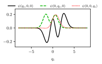
Figure 1: Select cross-sections of the three-dimensional initial wavepacket $\psi(q_{1},q_{2},q_{3})$.

The initial wavepacket, with a unit mass, was chosen to be the linear combination of the $(3,0,0)$ and $(1,2,1)$ basis functions with equal weights (see Figure 1 for cross-sections of the initial wavefunction). The associated Gaussian parameters corresponded to the ground state of another harmonic potential that is displaced, squeezed and rotated compared to the potential used for propagation (the parameters are available in the Supplementary material). The wavepacket was propagated for 2000 steps with a time step of 0.1 and the autocorrelation function was computed every five steps.

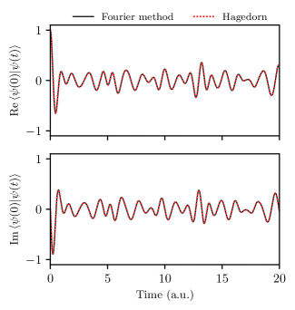
Figure 2: Comparison of the autocorrelation functions obtained with the split-operator Fourier method and Hagedorn approach.

Figure 2 shows that the autocorrelation function computed with the Hagedorn approach agrees perfectly with the autocorrelation function obtained with the split-operator Fourier method. In this example, the Fourier method required $32^{3}$ grid points to obtain a converged result, whereas the gridless Hagedorn wavepacket dynamics only needed the propagation of the five Gaussian parameters by solving a system of first-order ordinary differential equations. The Hagedorn approach can easily treat both the propagation and the computation of overlap integrals in much higher dimensions than the grid-based Fourier method whose cost grows exponentially with the number of degrees of freedoms.

6 Conclusions

We have discussed properties of Hagedorn functions and wavepackets associated with two different Gaussians. In particular, we have derived algebraic recurrence expressions for the overlap between two Hagedorn functions with different Gaussian centers and numerically demonstrated that both our expressions and their implementation are correct, efficient, and robust.

With these expressions available, Hagedorn wavepackets should find more applications in spectroscopy, particularly in situations where a non-Gaussian initial state is generated (e.g., in single vibronic level fluorescence [79] or Herzberg–Teller spectroscopy [80]) or where anharmonicity results in the occupation of excited Hagedorn functions.

Appendix A Special cases

The algebraic recursive expressions (97)–(98) for the overlaps are valid for any dimension $D$ and any excitation shells numbered by the total excitation $|J|$ and $|K^{\prime}|$. Here we describe how the general expressions simplify substantially if one is only interested in arbitrary excitations of one-dimensional systems or in low excitations of arbitrary-dimensional systems.

A.1 One-dimensional case

For $D=1$, the multi-indices become ordinary indices and the solutions (97)–(98) are:

$$M_{J+1,K^{\prime}} =\left[\sqrt{J+1}|U|^{2}\right]^{-1}(\bar{U}\sqrt{K^{\prime}}M_{J,K^{\prime}-1}-V\bar{U}\sqrt{J}M_{J-1,K^{\prime}}+wM_{JK^{\prime}}),$$ (111)

$$M_{J,K^{\prime}+1} =\left[\sqrt{K^{\prime}+1}|U|^{2}\right]^{-1}(\bar{V}\bar{U}\sqrt{K^{\prime}}M_{J,K^{\prime}-1}+\bar{U}\sqrt{J}M_{J-1,K^{\prime}}+w^{\prime}M_{JK^{\prime}}).$$ (112)

A.2 First shell in many dimensions

Let us evaluate the overlaps between the zeroth and first shells for any $D$. We set $J:=0$ and $K^{\prime}:=0$ in the general solutions (97) for $M_{J+\langle j\rangle,K^{\prime}}$ and (98) for $M_{J,K^{\prime}+\langle k\rangle}$ to find

$$M_{\langle j\rangle,0} =u_{j}M_{00},$$ (113)

$$M_{0,\langle k\rangle} =u_{k}^{\prime}M_{00},$$ (114)

where the scalar quantity

$$M_{00}:=M_{|J|=0,|K^{\prime}|=0}=\langle 0|0^{\prime}\rangle$$ (115)

is the overlap of the guiding Gaussians. In matrix form, the solution can be written as

$$M_{10} =uM_{00},$$ (116)

$$M_{01} =u^{\prime}M_{00},$$ (117)

where

$$M_{10}:=M_{|J|=1,|K^{\prime}|=0}\text{ \ \ and \ \ }M_{01}:=M_{|J|=0,|K^{\prime}|=1}\text{ }$$ (118)

are the $D$-vectors of overlaps between the zeroth and first shells.

To find overlaps of the first shells, we set $J:=0$ and $K^{\prime}:=\left\langle k\right\rangle$ in the general solution (97) for $M_{J+\langle j\rangle,K^{\prime}}$ and get

$$M_{\langle j\rangle,\langle k\rangle}=F_{jk}M_{00}+u_{j}M_{0,\langle k\rangle},$$ (119)

which, in matrix notation, becomes

$$M_{11} =FM_{00}+u\otimes M_{01}^{T}$$

$$=(F+u\otimes u^{\prime T})M_{00}$$ (120)

where

$$M_{11}:=M_{|J|=1,|K^{\prime}|=1}$$ (121)

is a $D\times D$ overlap matrix of the first shell functions. If $U$ itself is invertible, so is $U^{{\dagger}}$ since $(U^{{\dagger}})^{-1}=(U^{-1})^{{\dagger}}$. As a result, $W=U^{-1}\cdot(U^{{\dagger}})^{-1}$, $F=U^{-1}$, and

$$M_{11}\overset{U\text{ invertible}}{=}(U^{-1}+u\otimes u^{\prime T})M_{00}.$$ (122)

A.3 Second shell in many dimensions

To evaluate the overlap matrix $M_{20}$, let us set $J:=\langle j\rangle$, $j:=k$, $K^{\prime}:=0$, and $k:=l$ in the general expression (97) for $M_{J+\langle j\rangle,K^{\prime}}$ and find that

$$\sqrt{\delta_{jk}+1}M_{\langle j\rangle+\langle k\rangle,0}=(-GM_{00}+u\otimes M_{10}^{T})_{jk}=(-G+u\otimes u^{T})_{jk}M_{00}.$$ (123)

To compute the $3$-tensor $M_{21}$, we set $J:=\langle j\rangle$, $j:=k$, $K^{\prime}:=\langle l\rangle$, $k:=m$ in the expression (97) for $M_{J+\langle j\rangle,K^{\prime}}$ and find that

$$\sqrt{\delta_{jk}+1}M_{\langle j\rangle+\langle k\rangle,\langle l\rangle} =F_{kl}M_{\langle j\rangle,0}-G_{kj}M_{0,\langle l\rangle}+u_{k}M_{\langle j\rangle\langle l\rangle}$$

$$=[F_{kl}u_{j}-G_{kj}u_{l}^{\prime}+u_{k}(F+u\otimes u^{\prime T})_{jl}]M_{00}.$$ (124)

Note that the left-hand sides of equations for $M_{20}$ and $M_{21}$ are obviously symmetric w.r.t. exchange of $j$ and $k$. It may be numerically advantageous to take the symmetric average of the right-hand side of the corresponding equations.

To find $M_{02}$, let us set $J:=0$ and $K^{\prime}:=\langle j\rangle$ in the expression for $M_{J,K^{\prime}+\langle k\rangle}$:

$$\sqrt{\delta_{jk}+1}M_{0,\langle j\rangle+\langle k\rangle}=(G^{\prime}M_{00}+u^{\prime}\otimes M_{01}^{T})_{kj}=(G^{\prime}+u^{\prime}\otimes u^{\prime T})_{kj}M_{00}.$$ (125)

To find $M_{12}$, we set $J:=\langle j\rangle$, $K^{\prime}:=\langle k\rangle$, $k:=l$, $j:=m$ in the general expression for $M_{J,K^{\prime}+\langle k\rangle}$ and obtain

$$\sqrt{\delta_{kl}+1}M_{\langle j\rangle,\langle k\rangle+\langle l\rangle} =G_{lk}^{\prime}M_{\langle j\rangle,0}+F_{lj}^{\prime}M_{0,\langle k\rangle}+u_{l}^{\prime}M_{\langle j\rangle\langle k\rangle}$$

$$=[G_{lk}^{\prime}u_{j}+F_{lj}^{\prime}u_{k}^{\prime}+u_{l}^{\prime}(F+u\otimes u^{\prime T})_{jk}]M_{00}.$$ (126)

Finally, to find $M_{22}$ from $M_{12}$, let us set $J:=\langle j\rangle$, $K^{\prime}:=\langle k\rangle+\langle m\rangle$, $k:=r$, $j:=l$ in the general expression for $M_{J+\langle j\rangle,K^{\prime}}$:

$$\sqrt{\delta_{jl}+1}M_{\langle j\rangle+\langle l\rangle,\langle k\rangle+\langle m\rangle}$$

$$=\sum_{r=1}^{D}\left(F_{lr}\sqrt{\delta_{kr}+\delta_{mr}}M_{\langle j\rangle,\langle k\rangle+\langle m\rangle-\langle r\rangle}-G_{lr}\sqrt{\delta_{jr}}M_{\langle j\rangle-\langle r\rangle,\langle k\rangle+\langle m\rangle}\right)+u_{l}M_{\langle j\rangle,\langle k\rangle+\langle m\rangle}$$

$$=\sum_{r=1}^{D}\left(F_{lr}\sqrt{\delta_{kr}+\delta_{mr}}M_{\langle j\rangle,\langle k\rangle+\langle m\rangle-\langle r\rangle}\right)-G_{lj}M_{0,\langle k\rangle+\langle m\rangle}+u_{l}M_{\langle j\rangle,\langle k\rangle+\langle m\rangle}$$ (127)

It is convenient to distinguish cases $k=m$ and $k\neq m$:

$$\sqrt{\delta_{jl}+1}M_{\langle j\rangle+\langle l\rangle,\langle k\rangle+\langle m\rangle}\overset{k\neq m}{=}F_{lk}M_{\langle j\rangle,\langle m\rangle}+F_{lm}M_{\langle j\rangle,\langle k\rangle}-G_{lj}M_{0,\langle k\rangle+\langle m\rangle}+u_{l}M_{\langle j\rangle,\langle k\rangle+\langle m\rangle},$$ (128)

$$\sqrt{\delta_{jl}+1}M_{\langle j\rangle+\langle l\rangle,2\langle k\rangle}\overset{k=m}{=}F_{lk}\sqrt{2}M_{\langle j\rangle,\langle k\rangle}-G_{lj}M_{0,2\langle k\rangle}+u_{l}M_{\langle j\rangle,2\langle k\rangle}.$$ (129)

Data availability statement

All data that support the findings of this study are included within the article (and any supplementary files).

References

References

- [1] Heller E J 1975 J. Chem. Phys. 62 1544–1555
- [2] Heller E J 1981 Acc. Chem. Res. 14 368–375
- [3] Hagedorn G A 1981 Ann. Phys. (NY) 135 58–70
- [4] Herman M F and Kluk E 1984 Chem. Phys. 91 27–34
- [5] Ben-Nun M, Quenneville J and Martínez T J 2000 J. Phys. Chem. A 104 5161–5175
- [6] Worth G A, Robb M A and Burghardt I 2004 Faraday Discuss. 127 307–323
- [7] Beck M, Jäckle A, Worth G and Meyer H D 2000 Phys. Rep. 324 1–105
- [8] Miller W H 2001 J. Phys. Chem. A 105 2942
- [9] Werther M and Großmann F 2020 Phys. Rev. B 101 174315
- [10] Lasser C and Lubich C 2020 Acta Numerica 29 229–401
- [11] Vaníček J J L 2023 J. Chem. Phys. 159 014114
- [12] Heller E J 2018 The semiclassical way to dynamics and spectroscopy (Princeton, NJ: Princeton University Press)
- [13] Heller E J 1976 J. Chem. Phys. 64 63–73
- [14] Hellsing B, Sawada S I and Metiu H 1985 Chem. Phys. Lett. 122 303–309
- [15] Arickx F, Broeckhove J, Kesteloot E, Lathouwers L and Van Leuven P 1986 Chem. Phys. Lett. 128 310–314
- [16] Coalson R D and Karplus M 1990 J. Chem. Phys. 93 3919–3930
- [17] Lubich C 2008 From Quantum to Classical Molecular Dynamics: Reduced Models and Numerical Analysis 12th ed (Zürich: European Mathematical Society) ISBN 978-3037190678
- [18] Frantsuzov P A and Mandelshtam V A 2004 J. Chem. Phys. 121 9247–9256
- [19] Grossmann F 2006 J. Chem. Phys. 125 014111
- [20] Deckman J and Mandelshtam V A 2010 J. Phys. Chem. A 114 9820–9824
- [21] Cartarius H and Pollak E 2011 J. Chem. Phys. 134 044107
- [22] Wehrle M, Šulc M and Vaníček J 2014 J. Chem. Phys. 140 244114
- [23] Gottwald F, Ivanov S D and Kühn O 2019 J. Chem. Phys. 150
- [24] Begušić T, Cordova M and Vaníček J 2019 J. Chem. Phys. 150 154117
- [25] Golubev N V, Begušić T and Vaníček J 2020 Phys. Rev. Lett. 125 083001
- [26] Begušić T and Vaníček J 2020 J. Chem. Phys. 153 024105
- [27] Begušić T, Tapavicza E and Vaníček J 2022 J. Chem. Theory Comput. 18 3065–3074
- [28] Scheidegger A, Vaníček J and Golubev N V 2022 J. Chem. Phys. 156 034104
- [29] Moghaddasi Fereidani R and Vaníček J J L 2023 J. Chem. Phys. 159 094114
- [30] Moghaddasi Fereidani R and Vaníček J J L 2024 J. Chem. Phys. 160 044113
- [31] Poulsen J A and Nyman G 2024 Entropy 26 412
- [32] Gherib R, Ryabinkin I G and Genin S N 2024 Thawed Gaussian wavepacket dynamics with -machine learned potentials (Preprint arXiv:2405.00193)
- [33] Ryabinkin I G, Gherib R and Genin S N 2024 Thawed Gaussian wave packet dynamics: a critical assessment of three propagation schemes (Preprint arXiv:2405.01729)
- [34] Dirac P 1947 The Principles of Quantum Mechanics International series of monographs on physics (Clarendon Press)
- [35] Tannor D J 2007 Introduction to Quantum Mechanics: A Time-Dependent Perspective (Sausalito: University Science Books) ISBN 978-1891389238
- [36] Hagedorn G A 1985 Ann. Henri Poincaré 42 363–374
- [37] Hagedorn G A 1998 Ann. Phys. (NY) 269 77–104
- [38] Faou E, Gradinaru V and Lubich C 2009 SIAM J. Sci. Comp. 31 3027–3041
- [39] Gradinaru V, Hagedorn G A and Joye A 2010 J. Chem. Phys. 132 184108
- [40] Zhou Z 2014 J. Comput. Phys. 272 386–407
- [41] Gradinaru V and Rietmann O 2021 J. Comput. Phys. 445 110581
- [42] Hagedorn G A 2013 A minimal uncertainty product for one dimensional semiclassical wave packets Spectral Analysis, Differential Equations and Mathematical Physics: A Festschrift in Honor of Fritz Gesztesy’s 60th Birthday (Proceedings of Symposia in Pure Mathematics vol 87) ed Holden H, Simon B and Teschl G (Providence, Rhode Island: American Mathematical Society) p 183
- [43] Ohsawa T and Leok M 2013 J. Phys. A 46 405201
- [44] Gradinaru V and Hagedorn G A 2014 Numer. Math. 126 53–73
- [45] Lasser C and Troppmann S 2014 J. Fourier Anal. Appl. 20 679–714
- [46] Li X and Xiao A 2014 International Journal of Modeling, Simulation, and Scientific Computing 05 1450013
- [47] Hagedorn G A 2015 Ann. Phys-new. York. 362 603–608
- [48] Ohsawa T 2015 J. Math. Phys. 56 032103
- [49] Punoševac P and Robinson S L 2016 J. Math. Phys. 57 092102
- [50] Dietert H, Keller J and Troppmann S 2017 J. Math. Anal. Appl. 450 1317–1332
- [51] Bourquin R 2017 Numerical Algorithms for Semiclassical Wavepackets Ph.D. thesis ETH Zürich
- [52] Hagedorn G A and Lasser C 2017 SIAM J. Matrix Anal. Appl. 38 1560–1579
- [53] Lasser C, Schubert R and Troppmann S 2018 J. Math. Phys. 59 082102
- [54] Ohsawa T 2018 Nonlinearity 31 1807–1832
- [55] Punoševac P and Robinson S L 2019 J. Math. Phys. 60 052106
- [56] Ohsawa T 2019 J. Fourier Anal. Appl. 25 1513–1552
- [57] Blanes S and Gradinaru V 2020 J. Comput. Phys. 405 109157
- [58] Arnaiz V 2022 J. Spectr. Theory 12 745–812
- [59] Miao B, Russo G and Zhou Z 2023 IMA J. Numer. Anal. 43 1221–1261
- [60] Kargol A 1999 Annales de l’I.H.P. Physique théorique 71 339–357
- [61] Hagedorn G and Joye A 2000 Ann. Henri Poincaré 1 837–883
- [62] Gradinaru V, Hagedorn G A and Joye A 2010 J. Phys. Math. Theor. 43 474026
- [63] Gradinaru V, Hagedorn G A and Joye A 2010 J. Chem. Phys. 132 184108
- [64] Kieri E, Holmgren S and Karlsson H O 2012 J. Chem. Phys. 137 044111
- [65] Bourquin R, Gradinaru V and Hagedorn G A 2012 J. Math. Chem. 50 602–619
- [66] Gradinaru V and Rietmann O 2024 J. Comput. Phys. 509 113029
- [67] Wehrle M, Oberli S and Vaníček J 2015 J. Phys. Chem. A 119 5685
- [68] Begušić T and Vaníček J 2020 J. Chem. Phys. 153 184110
- [69] Prlj A, Begušić T, Zhang Z T, Fish G C, Wehrle M, Zimmermann T, Choi S, Roulet J, Moser J E and Vaníček J 2020 J. Chem. Theory Comput. 16 2617–2626
- [70] Begušić T and Vaníček J 2021 Chimia 75 261
- [71] Klētnieks E, Alonso Y C and Vaníček J J L 2023 J. Phys. Chem. A 127 8117–8125
- [72] Ma X and Rhodes W 1990 Phys. Rev. A 41 4625–4631
- [73] Harris C R, Millman K J, van der Walt S J, Gommers R, Virtanen P, Cournapeau D, Wieser E, Taylor J, Berg S, Smith N J, Kern R, Picus M, Hoyer S, van Kerkwijk M H, Brett M, Haldane A, del Río J F, Wiebe M, Peterson P, Gérard-Marchant P, Sheppard K, Reddy T, Weckesser W, Abbasi H, Gohlke C and Oliphant T E 2020 Nature 585 357–362
- [74] Virtanen P, Gommers R, Oliphant T E, Haberland M, Reddy T, Cournapeau D, Burovski E, Peterson P, Weckesser W, Bright J, van der Walt S J, Brett M, Wilson J, Millman K J, Mayorov N, Nelson A R J, Jones E, Kern R, Larson E, Carey C J, Polat İ, Feng Y, Moore E W, VanderPlas J, Laxalde D, Perktold J, Cimrman R, Henriksen I, Quintero E A, Harris C R, Archibald A M, Ribeiro A H, Pedregosa F, van Mulbregt P and SciPy 10 Contributors 2020 Nat. Methods 17 261–272
- [75] Piessens R, de Doncker-Kapenga E, Überhuber C W and Kahaner D K 1983 QUADPACK: A subroutine package for automatic integration (Springer Verlag)
- [76] Feit M D, Fleck Jr J A and Steiger A 1982 J. Comp. Phys. 47 412
- [77] Kosloff D and Kosloff R 1983 J. Comp. Phys. 52 35–53
- [78] Roulet J, Choi S and Vaníček J 2019 J. Chem. Phys. 150 204113
- [79] Tapavicza E 2019 J. Phys. Chem. Lett. 10 6003–6009
- [80] Patoz A, Begušić T and Vaníček J 2018 J. Phys. Chem. Lett. 9 2367–2372