Accelerating the prediction of stacking fault energy by combining ab initio calculations and machine learning

Abstract

Stacking fault energies (SFEs) are key parameters to understand the deformation mechanisms in metals and alloys, and prior knowledge of SFEs from ab initio calculations is crucial for alloy designing. Machine learning (ML) algorithms used in the present work show a $\sim$80 times acceleration of generalized stacking fault energy (GSFE) predictions, which are otherwise computationally very expensive to get directly from density functional theory (DFT) calculations, particularly for alloys. The origin of the features used for training the ML algorithms lies in the physics-based Friedel model, and the present work uncovers the connection between the physics of d-electrons and the deformation behavior of transition metals and alloys. Predictions based on the ML model agree with the experimental data. Our model can be helpful in accelerated alloy designing by providing a fast method of screening materials in terms of stacking fault energies.

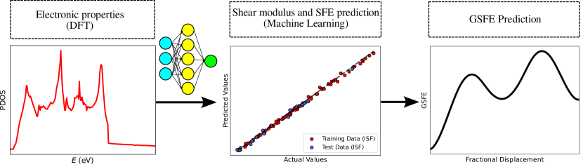
Figure 1: Workflow for physics based accelerated generalized stacking fault energy (GSFE) calculation: ab initio electronic density of states (DOS) calculation, followed by machine learning based prediction of stacking fault energy and GSFE curve.

I Introduction

Stacking fault (SF) in face-centered cubic (FCC) materials is a planar defect that arises during plastic deformation through dissociating a perfect dislocation into two Shockley partial dislocations. Stacking fault energy (SFE) is a crucial parameter that determines the deformation mechanisms of FCC materials. Materials with low-to-medium SFE generally deform via transformation-induced plasticity (TRIP) or twinning-induced plasticity (TWIP), while those with high SFE deform via dislocation slip. SFE depends on several parameters like temperature [1, 2] and stress [3, 4] and it can be tuned via alloying [5, 6, 7, 8]. Since SFE dictates dislocation dissociation, it is one of the determining factors for the dislocation pile-up at the twin boundaries (TBs), resulting in fatigue cracking [9]. Deformation processing (like ball milling, rolling, and torsion) or lattice mismatch-induced interface strain can form high-density SFs in low-to-medium SFE metals, leading to strain hardening while maintaining good ductility [10]. SFE plays a major role in the mechanical properties of bulk nanostructured materials processed via severe plastic deformation [11]. The creep life of Ni-based superalloys improves due to SFE reduction by alloying with Co [12]. Due to its importance in the mechanical behavior of metals, several experimental and computational methods have been developed for SFE estimation, as discussed below.

Experimentally, SFEs are estimated by transmission electron microscopy (TEM) or by X-ray diffraction (XRD) and neutron diffraction (ND). Using TEM, the intrinsic SFE is estimated by measuring the stacking fault width, which is defined as the separation distance of isolated pairs of leading and trailing partial dislocations. This method assumes a balance between the excess energy stored in the stacking fault and the elastic strain energy responsible for the mutual repulsion of leading and trailing partials [13]. The determination of SFE through XRD and ND involves analyzing the shift and broadening of the Bragg peak, considering the relationship between stacking fault probability, dislocation density, and intrinsic SFE [14]. An in situ XRD method to measure the critical stress in the early stage of plastic deformation provides another way of estimating SFE experimentally [15, 16].

The experimental methods mentioned above have one limitation - SFE at any unstable point (lying between perfect and faulted crystal) cannot be estimated. Such curves with SFE values at multiple points between perfect and faulted crystals are known as the generalized stacking fault energy (GSFE) profile or $\gamma$ surface. Computational methods like DFT or classical molecular dynamics (MD) are used to calculate the $\gamma$ surface [17, 18, 19, 4, 20, 21]. The $\gamma$ surface represents the potential energy landscape between adjacent planes in a slip system. Simulated $\gamma$ surface acts as an input for calculating the Peierls stresses via the Peierls-Nabarro model (P-N model) for studying dislocations [22, 23, 24, 25, 26, 27, 28, 27, 29, 30], plastic deformation in high entropy alloys [31, 32] and phase transitions [33, 34]. Due to its ab initio nature, $\gamma$ surface predicted by DFT is believed to be very accurate, and the SFE values are in reasonable agreement with experimental findings. However, DFT calculation predicts negative SFEs for some materials like metastable alloys, which are experimentally reported to have small but positive SFE [35, 36, 37, 38, 39, 40, 41]. Several attempts have been made to understand the reasons behind the discrepancy, further establishing the reliability of DFT for SFE prediction [14, 42].

Accuracy and reliability of DFT for SFE prediction lies in its ability to accurately incorporate the effect of electronic contributions [43, 44, 45, 46, 47, 48, 49]. For example, I. R. Harris et al. showed the connection between the electronic structure (empty d-states) and SFE [50]. Datta et al. found that the electronic density of states (DOS) plots for the faulted structures are considerably smoother compared to the pristine materials [51]. A study on the influence of solute substitutions in Ni on its GSFE found a correlation between density of state (DOS) and intrinsic stacking fault (ISF) energy [52]. The energy barriers for both deformation slip and twinning formation decrease with the increased electron concentrations in ZnS, ZnTe, and CdTe [53]. A recent study also revealed a direct correlation of SFE with the width of the d-band of FCC transition metals [4]. As suggested by the previous studies, a deep connection exists between the electronic band structure and SFE, which we would like to explore in detail in the present work.

In contemporary times, machine learning (ML) algorithms have emerged as practical tools capable of achieving robust predictive outcomes for a given input dataset. Recent reports highlight the application of ML in several domains of materials science and engineering, like potential development [54], microstructure modeling [55], and structure-property correlation [56, 57]. In alloy development, ML has been employed for predicting phase stability, glass forming ability, and properties as a function of alloy composition [58, 59, 60]. Stacking fault energy, the subject matter of this paper has also been predicted using ML models using local composition, atomic size, electronic structure, physical, thermomechanical, and elastic properties as descriptors [61, 62, 63, 64, 65, 66]. However, it is noteworthy that the values of these fundamental properties for alloys are often estimated using the rule of mixture, introducing potential discrepancies in the results. A few studies have attempted to predict SFE using charge density obtained from DFT calculations [67, 68].

The novelty of the present work lies in its use of the physics-based Friedel model for deriving the features for machine learning. The physics-based model helps us to uncover the connection between the SFE and electronic band structure of FCC transition metals and alloys. A schematic diagram is illustrated in Figure 1. First, we calculate the electronic density of states (DOS), a routine job for DFT packages. Using the electronic DOS data, we calculate some parameters like the width of the d-band (W_d), energy at the band center ($\varepsilon_{d}$), electrons in the d-orbital (z_d), and electrons in the s-orbital (z_s). Using various machine learning models [Gaussian process regression (GPR), support vector regression (SVR), deep neural network (DNN), and random forest], we are able to predict the stacking fault energy and shear modulus of transition metals and alloys using the parameters obtained from DOS. Values predicted by the ML models agree with the experimental data. We are also able to predict the GSFE curve with reasonable accuracy, and our combined ab initio-ML approach can accelerate the GSFE calculation 80x faster compared to solely ab initio based approach in the case of alloys. Our work paves the way for fast and accurate computational prediction of transition metal alloys with desired SFE values, providing a valuable understanding of the deformation mechanism and mechanical behavior.

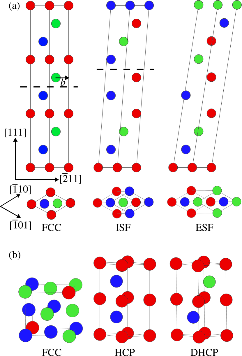
Figure 2: (a) Supercell method: side view (first row) and top view (second row) of the supercell of the face centered cubic or FCC (left), intrinsic stacking fault or ISF (center) and extrinsic stacking fault or ESF (right). Starting from the FCC structure, all the atoms located above the dotted line and the out-of-plane cell vector are displaced by $\vec{b}$ (2$\vec{b}$) to go from the FCC to ISF (ESF) structure. (b) ANNNI model: FCC, hexagonal closed packed or HCP and double hexagonal closed packed or DHCP cells used for the stacking fault energy calculations. In both (a) and (b) the A, B and C stacking sequence of atoms along the closed packed direction are represented in red, blue and green colors respectively.

II Methodology

Density functional theory (DFT) calculations, as implemented in the Vienna Ab-initio Simulation Package (VASP) [69], are performed using a plane wave basis set (with a 400 eV kinetic energy cut-off) and projector augmented wave (PAW) potentials [70]. The generalized gradient approximation (GGA), applying Perdew, Burke, and Ernzerhof (PBE) as exchange-correlation functional [71], is used. The unit cell parameters and atomic coordinates are fully relaxed until the energy converges to within $10^{-6}$ eV and the atomic force dips below 0.01 eV/Å. Further details about the supercell size and k-point mesh used for Brillouin zone sampling are given in the respective sections.

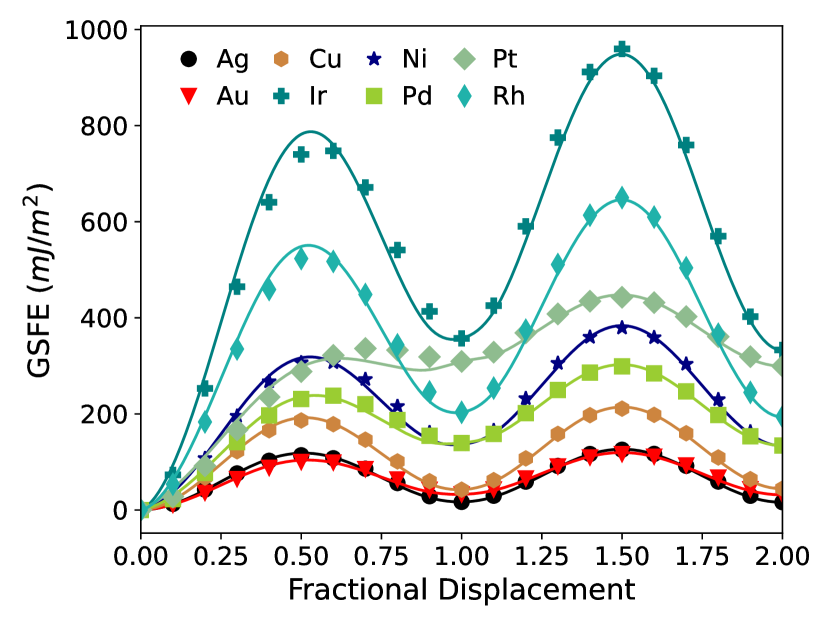
Figure 3: Generalized stacking fault energy (GSFE) curves for FCC metals, illustrated along the $[\overline{2}11]$ direction. Energy values are plotted from 0 to $2\vec{b}$, where Bergers vector $\vec{b}=\frac{1}{6}[\overline{2}11]$. Symbols depict DFT values, while the curves are fitted using Equation 2.

III Results and discussion

III.1 Stacking fault energy calculations

Table 1: Comparison of SFEs obtained from DFT using two approaches (supercell and ANNNI model), predicted SFEs (using deep neural network or DNN) and experimental data [72]^a, [73]^b, [74]^c. A similar comparison for shear modulus values obtained through DFT, predicted using DNN and experimental values [75]^d. Both DFT and ML-predicted values are in good agreement with the experimental values.

Metals	DFT					Predicted			Exp.
	Supercell		ANNNI		G	$\gamma_{ISF}$	$\gamma_{ESF}$	G	$\gamma_{ISF}$	Gd
	$\gamma_{ISF}$	$\gamma_{ESF}$	$\gamma_{ISF}$	$\gamma_{ESF}$
Ag	16.9	16.3	17.5	18.4	22.0	18.1	23.2	22.8	25.0a	27.0
Au	32.6	31.7	23.6	23.3	15.4	32.8	37.5	19.2	45.0a	27.7
Cu	42.4	44.6	48.7	53.3	49.8	43.8	56.3	39.6	55.0b	48.3
Ir	357.2	333.1	348.3	334.3	214.4	359.6	400.3	216.1	480.0c	210.0
Ni	136.6	133.9	140.8	135.0	95.1	138.5	162.7	95.1	125.0c	75.0
Pd	139.5	134.3	146.6	139.5	44.4	137.1	148.3	45.1	130.0a	43.6
Pt	309.1	299.5	277.0	282.6	48.6	299.8	315.6	50.6	322.0c	61.0
Rh	203.4	194.3	190.2	188.2	146.8	207.0	240.4	150.5	330.0a	150.0
Pd-Pt	190.8	180.9	176.0	172.0	45.8	172.2	186.5	47.0	-	-
Ir-Pt	359.5	342.9	328.5	326.2	163.5	326.6	371.5	150.5	-	-
Pd-Au	131.4	128.2	118.0	112.0	37.4	116.0	123.9	37.5	-	-

III.1.1 SFE using periodic supercell

We consider an ideal FCC structure composed of 9 layers stacked in an …ABCABCABC… pattern [Figure 2(a)]. Two of the cell vectors, $\frac{1}{2}[\overline{1}10]$ and $\frac{1}{2}[\overline{1}01]$, lie on the (111) plane, while the third one is perpendicular to the (111) plane and aligned along the [111] direction. An intrinsic stacking fault (ISF) has a stacking sequence of …ABCABABCABC…, as shown in Figure 2(a).

An ISF is created by fixing the bottom five layers and displacing each of the top four layers by the Burgers vector $\vec{b}=\frac{1}{6}[\overline{2}11]$. Simultaneously, we shift the out-of-the-plane cell vector (oriented initially along the [111] direction) by the same vector $\vec{b}$ to preserve the unit cell’s periodicity. This approach enables us to compute the stacking fault energy using periodic cells, eliminating the need for introducing surface layers [76]. We define the intrinsic stacking fault energy $\gamma_{ISF}$ as the energy difference between the faulted and ideal structures per unit area:

$$\gamma_{ISF}=\frac{E_{ISF}-E_{FCC}}{A}.$$ (1)

To get the energy values for metals from DFT calculations, we use $21\times 21\times 2$ k-point mesh.

An extrinsic stacking fault (ESF) has a stacking sequence of …ABCABACABC…, as shown in Figure 2(a). Starting with the ISF structure, we now fix the bottom six layers and displace the top three layers by $\vec{b}=\frac{1}{6}[\overline{2}11]$. The out-of-the-plane cell vector is also shifted by $\vec{b}$, yielding the ESF stacking sequence [Figure 2(a)]. Notably, in the case of ESF, the top 3 layers and the out-of-the-plane cell vector are displaced by $2\vec{b}$ relative to the ideal FCC configuration. To determine the $\gamma_{ESF}$ value, we employ an expression similar to Equation 1.

Apart from the $\gamma_{ISF}$ and $\gamma_{ESF}$, we compute stacking fault energies at various displacements, ranging from 0 to $2b$, with a step size of $0.1b$ to delineate the entire GSFE curve, as shown in Figure 3. Two significant peaks along the GSFE curve are noteworthy—one situated at approximately the middle of ideal FCC and ISF (referred to as the unstable stacking fault or USF), and the other located at approximately the middle of ISF and ESF (referred to as the unstable twinning fault or UTF). These peaks represent the energy barriers for forming ISF and ESF, respectively.

We illustrate the GSFE curves of all the transition and noble metals having FCC ground state in Figure 3. The symbols in the figure represent the values calculated from DFT. The curves are drawn using the following expressions:

$$\small\gamma=\begin{cases}cG\sin^{2}(\pi x)+\gamma_{ISF}\cdot x,&0\leq x\leq 1\\ cG\sin^{2}(\pi x)+\gamma_{ISF}\cdot(2-x)+\gamma_{ESF}\cdot(x-1),&1\leq x\leq 2\end{cases}$$ (2)

where $\gamma_{ISF}$, $\gamma_{ESF}$ and shear modulus $G$ are calculated from DFT, $c$ is a constant, and $x$ is the fractional displacement in terms of Burgers vector $\vec{b}$. The values of $c$ are 5.01 for Ag, 5.67 for Au, 3.43 for Cu, 3.74 for Pd, 2.96 for Pt, 2.61 for Ni, 3.04 for Rh, and 2.81 for Ir. We calculate the shear modulus via strain-energy approach [77] by using VASPKIT tool [78], details of which are given in Section I, Supplemental Material (SM) [79]. In conclusion, one can generate the entire GSFE curve with reasonable accuracy by calculating three numbers: $\gamma_{ISF}$, $\gamma_{ESF}$, and $G$ from DFT. Such an approach is computationally cheaper than calculating the entire GSFE curve from DFT, particularly when dealing with alloys.

III.1.2 SFE using ANNNI model

Axial-next-nearest-neighbor ising (ANNNI) model is an alternate route for finding SFEs. Although the model is computationally less expensive, one can get only the ISF and ESF values instead of the entire GSFE curve. ANNNI model uses specific combinations of energies corresponding to different short-period stacking sequences of close-packed (111) planes. For example, the second-order approximation to obtain the ISF and ESF energies is given by the following combinations:

$$E_{ISF}=\frac{E_{HCP}+2E_{DHCP}-3E_{FCC}}{A},$$ (3)

$$E_{ESF}=\frac{4(E_{DHCP}-E_{FCC})}{A}.$$

In the above equation, $A=\frac{\sqrt{3}}{4}a^{2}$, where $a$ is the lattice parameter of a conventional FCC unit cell. Energies of the face-centered cubic (ABCABC stacking), hexagonal close-packed (ABAB stacking), and double hexagonal close-packed (ABACABAC stacking) structures are denoted by $E_{\text{FCC}}$, $E_{\text{HCP}}$, and $E_{\text{DHCP}}$, respectively. FCC, HCP, and DHCP unit cells used for the SFE calculation using the ANNNI model are illustrated in Figure 2(b). To get the energy values for metals from DFT calculations, we use $12\times 12\times 12$, $21\times 21\times 5$, and $21\times 21\times 5$ k-point mesh for FCC, HCP, and DHCP, respectively. SFE values calculated from the supercell method and ANNNI model are compared in Table 1. Besides Au, values obtained from both models are in remarkable agreement.

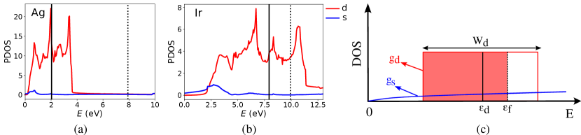
Figure 4: Orbital projected density of states for (a) Ag (completely full narrow d-band, low SFE) and (b) Ir (partially full wide d-band, high SFE). The black solid line denotes the d-band center ($\varepsilon_{d}$), while the dotted line represents the Fermi energy ($E_{F}$). (c) Schematic s-band and d-band electronic density of states, according to the Freidel model.

III.2 Friedel model

Understanding electronic structure is the primary building block for a comprehensive study of the material’s properties. Electrons serve as the quantum glue that keeps the nuclei of a solid together and influences the mechanical, electrical, optical, and magnetic properties of materials. It is well known that d-electrons play a significant role in transition metals’ electronic and magnetic properties. Figures 4(a)-(b) illustrate the DOS of s-electrons and d-electrons of Ag and Ir, respectively. Unlike the DOS of s-states, the DOS of d-states is sharply peaked, which indicates that d-states are relatively localized compared to the s-states. Although the DOS curves are quite intricate, Friedel proposed a significant simplification. The DOS of s-states, denoted by $g_{s}(\varepsilon)$, is approximated to be free electron like, obeying $g_{s}(\varepsilon)\propto\sqrt{\varepsilon}$ [Figure 4(c)]. The DOS of d-states, denoted by $g_{d}(\varepsilon)$, is approximated to be a step function [Figure 4(c)], expressed as,

$$g_{d}\left(\varepsilon\right)=\dfrac{10}{W_{d}},\hskip 28.45274pt\varepsilon_{d}-\dfrac{W_{d}}{2}<\varepsilon<\varepsilon_{d}+\dfrac{W_{d}}{2}$$ (4)

$$=0.\hskip 96.73918pt\rm{otherwise}.$$

The center of the d-band and its width are denoted by $\varepsilon_{d}$ and $W_{d}$, which are related to the projected density of states (PDOS) of the d-band. The first moment of DOS with respect to the Fermi energy ($\varepsilon_{F}$) is,

$$\mu=\int(\varepsilon-\varepsilon_{F})g^{DFT}_{d}(\varepsilon)d\varepsilon,$$ (5)

where $g^{DFT}_{d}(\varepsilon)$ is the PDOS of d-band, obtained from the ab initio calculations. The number $\varepsilon_{d}=(\varepsilon_{F}-|\mu|)$ corresponds to the center of the d-band. Further, we calculate the second moment of the DOS with respect to $\varepsilon_{d}$,

$$\sigma^{2}=\int(\varepsilon-\varepsilon_{d})^{2}g^{DFT}_{d}(\varepsilon)d\varepsilon.$$ (6)

We define the width of the d-band as $W_{d}$ = $2\sigma$. As shown in Figure S1 and S2 in SM, the periodic trend of calculated $\varepsilon_{d}$ and $W_{d}$ agree with the solid-state table [80].

It is evident that, unlike s-states, d-states can not be treated using free electron theory, and a tight binding-like description would be more appropriate. In a tight binding description, bandwidth is an important parameter that depends on the overlap of atomic orbitals. For example, core states have zero width because of no overlap. Valence d-states have a finite width, leading to some energy gain, depending on $W_{d}$. Using the DOS expression in Equation 4, one can illustrate that the energy gain is,

$$E_{d}=5W_{d}\left[-\dfrac{z_{d}}{10}+\left(\dfrac{z_{d}}{10}\right)^{2}\right],$$ (7)

where $z_{d}$ is the number of electrons in the d-band. We compute $z_{d}$ from the ab initio calculations by integrating the d-band PDOS up to the Fermi energy. We obtain $W_{d}$ from ab initio calculations using Equation 6. We define $E_{d}$ as the cohesive energy due to the overlap of adjacent d-bands. The term within the square bracket in Equation 7 has a minimum at $z_{d}=5$ (middle of the transition metal series), and it is zero at $z_{d}=10$ (noble metal). Our ab initio calculations confirm that $z_{d}$ increases as we move from left to right of a row in the periodic table [Figure S3 in SM]. However, $z_{d}$ is slightly less than 10 in noble metals, as some electrons are transferred to the free electron-like band. Interestingly, we also find a periodic trend in $W_{d}$ along a particular row; values increase from the left to the center and decrease from the center to the noble metal. In other words, $W_{d}$ has a maximum near the middle of the transition metal series [Figure S2 in SM]. According to the Friedel model, the binding energy [Equation 7] of transition metals is maximum near the middle of a row [Figure S4 in SM]. This trend is in reasonably good agreement with experimental values. For example, the melting point is higher near the middle of the transition metal series [Figure S4 in SM]. Such a correlation makes the Friedel model credible despite its simplicity.

We calculate the Wigner-Seitz radius $r_{0}$ by equating volume per atom (obtained from ab initio) to $4\pi r_{0}^{3}/3$. Values of $r_{0}$ obtained from ab initio agree well with the ones reported in the solid state table [Figure S5, SM]. Since d-band overlap decreases with increasing distance between the atoms, we assume bandwidth $W_{d}\propto r_{0}^{-\alpha}$. As a result, volume dependence of $E_{d}$, denoted by $\kappa_{d}$, can be expressed as,

$$\kappa_{d}=\frac{\partial E_{d}}{\partial r_{0}}=\frac{5\alpha W_{d}}{r_{0}}\left[\dfrac{z_{d}}{10}-\left(\dfrac{z_{d}}{10}\right)^{2}\right].$$ (8)

Similar to $E_{d}$, $\kappa_{d}$ also peaks near the middle of the transition metal series [Figure S6, SM].

In summary, the Friedel model defines binding among d-electrons in terms of specific material parameters, which can be computed from the electronic density of states obtained from ab initio calculations. In the following section, we use these parameters to fit a machine learning model, which can predict SFE values of transition metals and binary alloys.

III.3 Machine learning

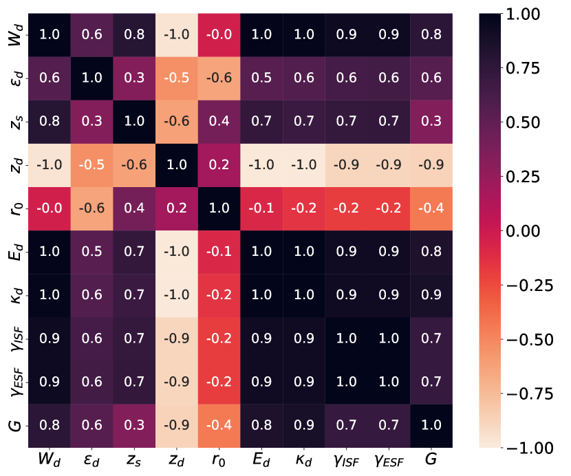
Figure 5: Heatmap of Pearson correlation coefficient matrix: target variables are $\gamma_{ISF},\gamma_{ESF},G$ and feature variables are $W_{d},\varepsilon_{d},z_{s},z_{d},r_{0},E_{d},\kappa_{d}$. Values close to black (white) indicate strongly positive (negative) correlations.

III.3.1 Data generation using ANNNI model

We use the ANNNI model to generate an extensive database of $\gamma_{ISF}$ and $\gamma_{ESF}$ values for Au-Pd, Pd-Ag, Ag-Au, Rh-Pd, Ir-Pd, Pd-Pt, Cu-Pt, Ir-Pt, Ni-Ag, Ni-Au, Ni-Pd, Ni-Pt, Ni-Rh and Ni-Cu binary alloys. These alloys are selected because of the solid solubility of the two elements throughout the composition range, spanning from 12.5% to 87.5%, with intervals of 12.5%, encompassing seven compositions for each alloy. Using the ATAT package [81], we generate special quasirandom structures (SQS) to describe the random arrangement of constituent atoms in a binary alloy. We generate three types of supercells, each containing 32 atoms: a conventional $2\times 2\times 2$ FCC supercell, a $2\times 2\times 4$ HCP supercell, and a $2\times 2\times 2$ DHCP supercell. We use a k-point mesh of $12\times 12\times 12$ for FCC, $21\times 21\times 5$ for HCP and DHCP supercell. The complete dataset for training and testing the ML model contains $\gamma_{ISF}$, $\gamma_{ESF}$ and $G$ values for 8 metals and all the binary alloys mentioned above. We also calculate the d-band PDOS and related parameters [Figure 4(c)] using the FCC supercell of the metals and alloys.

III.3.2 Feature and model selection

We aim to train a model to predict $\gamma_{ISF},\gamma_{ESF}$ and $G$ of a material from its DOS, such that one can generate the GSFE curves using Equation 2. For the purpose of prediction, we use $\varepsilon_{d},W_{d},z_{d},r_{0}$, and $z_{s}$ (number of s-electrons) as feature variables. Except $r_{0}$, the rest of the features have moderate to high values of correlation coefficients [Figure 5]. Notably, $z_{d}$ (number of d-electrons) has a very high negative correlation with SFEs, which implies lower SFE for a material with higher $z_{d}$. This observation agrees with the experimental facts that noble metals (Au, Ag, Cu) have low SFEs, as they have the highest d-electrons. Bandwidth $W_{d}$ has a very high positive correlation with SFEs, which is again consistent with the fact that noble metals have narrow bands compared to others [Figure 4 and Figure S7, S8 in SM], resulting in low SFEs.

Although some features have high correlation coefficients, a multivariable linear regression fails to predict the target variables accurately. Thus, we use other regression methods like deep neural network (DNN), support vector regression (SVR), Gaussian process regression (GPR), and random forest. We split the data set for training and testing (80:20). The latter is used to test the trained model and compute the test error. The mean absolute error between the actual and predicted values gives the loss. We select the model that exhibits the highest coefficient of determination for total average $R^{2}$ for the test set and the highest total $R^{2}$ for the training set as the optimal one for each approach. The following discussion covers DNN and random forest, while SVR and GPR are given in Section II and Figure S9, SM.

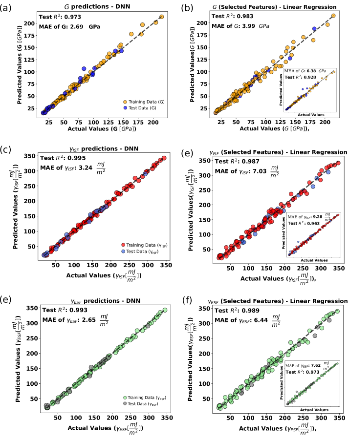
Figure 6: Panels (a), (c) and (e) illustrate the comparison between actual and predicted values from DNNs for $G$, $\gamma_{ISF}$ and $\gamma_{ESF}$, respectively. Panels (b), (d), and (f) depict the same for selected features using Equations 9, 10 and 11, while the insets illustrate the outcomes of random forest regression with all the features.

III.3.3 Deep neural network

DNNs can capture highly non-linear relationships and complex patterns because of their highly flexible and expressive interconnected architecture [82]. We evaluate the performance of different activation functions, like rectified linear unit (ReLU), leaky ReLU, and parametric ReLU (PReLU). PReLU demonstrates superior overall performance, achieving the highest accuracy among the tested activation functions with a test $R^{2}$ of 0.995 for $\gamma_{ISF}$ prediction, compared to leaky ReLU (0.993) and traditional ReLU (0.988). The neural network with PReLU activation showcases enhanced resistance to sample bias because of its adaptive nature to effectively modulate activation for negative inputs and minimize outliers’ impact while promoting superior generalization for a more reliable and stable predictive model than leaky ReLU and ReLU counterparts. Figure 6 (a), (c), (e) shows the predicted vs. actual values for the best models of DNN, which we train with 5-7 dense layers with a learning rate of $10^{-3}$ with around 200-500 epochs for iterations. We evaluate the model’s performance based on the test error and the change in loss with the iterations. Convergence with the number of iterations is shown in Figure S10, SM. The test $R^{2}$ values of $G$, $\gamma_{ISF}$ and$\gamma_{ESF}$ are 0.973, 0.995 and 0.993, respectively. The mean absolute errors (MAEs) of $G$, $\gamma_{ISF}$ and$\gamma_{ESF}$ are 2.69 GPa, 3.24 mJ/m² and 2.65 mJ/m², respectively.

III.3.4 Random forest

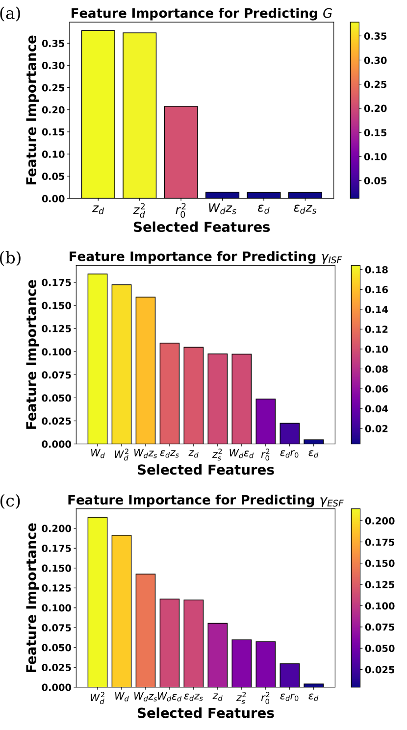
Figure 7: Feature importance plot for $G$, $\gamma_{ISF}$, and $\gamma_{ESF}$.

While the DNN exhibited impressive accuracy in predicting, it is not possible to understand how $\gamma_{ISF},\gamma_{ESF}$, and $G$ depend on the feature variables. Our next objective is to predict the expression for $\gamma_{ISF},\gamma_{ESF}$ and $G$ in terms of the feature variables. For this purpose, one must perform high-order polynomial regression, such as quadratic regression. This method expands the sample space from the initial five parameters ($\varepsilon_{d},W_{d},z_{d},r_{0}$, and $z_{s}$) to twenty parameters by incorporating quadratic combinations. However, employing this approach may introduce redundant parameters, potentially leading to overfitting.

A strategy to mitigate overfitting is to utilize a random forest regressor, incorporating the quadratic terms. The advantage of employing random forest lies in its ability to perform regression and simultaneously provide insights into the minimum number of terms essential for optimal prediction without the issue of overfitting by performing a search using its randomly ensembled decision trees. This process is called feature importance analysis. Details of feature importance analysis using random forest are given in Section III, SM. After feature importance analysis, we select only six terms for shear modulus prediction and ten terms for SFE prediction [Figure 7]. Finally, we do a multivariable linear regression with the selected features to obtain the following expressions, which can be directly used for prediction.

$$G=51.07z_{d}^{2}-63.21r_{0}^{2}+25.82\varepsilon_{d}$$ (9)

$$-876.15z_{d}+33.80W_{d}z_{s}-60.14\varepsilon_{d}z_{s}+3877.91.$$

$$\gamma_{\text{ISF}}=-22.66W_{d}^{2}-579.36z_{s}^{2}-522.06r_{0}^{2}-220.46\varepsilon_{d}$$ (10)

$$+27.77z_{d}+64.57W_{d}+18.51W_{d}\varepsilon_{d}+278.81W_{d}z_{s}$$

$$-49.31\varepsilon_{d}z_{s}+74.77\varepsilon_{d}r_{0}+996.58.$$

$$\gamma_{\text{ESF}}=-21.29W_{d}^{2}-730.97z_{s}^{2}-453.58r_{0}^{2}-178.69\varepsilon_{d}$$ (11)

$$+31.77z_{d}+78.59W_{d}+16.30W_{d}\varepsilon_{d}+249.45W_{d}z_{s}$$

$$+0.80\varepsilon_{d}z_{s}+41.06\varepsilon_{d}r_{0}+781.64.$$

Note that, before applying the feature importance selection analysis, the mean absolute error obtained by including all the twenty terms are 6.38 GPa, 9.28 mJ/m², and 7.62 mJ/m² for G, $\gamma_{ISF}$ and $\gamma_{ESF}$ [insets of Figure 6 (b), (d), (f)], which reduces to 3.99 GPa, 7.03 mJ/m², and 6.44 mJ/m² [Figure 6 (b), (d), (f)], respectively. The test $R^{2}$ values of $G$, $\gamma_{ISF}$ and$\gamma_{ESF}$ also improve from 0.928, 0.963, and 0.973 (with all twenty features) to 0.983, 0.987 and 0.989 (with selected features), respectively. The improvement can be attributed to keeping only essential features, thus reducing the problem of overfitting.

Figure 7 illustrates all the selected features that are utilized in predicting the formula [Equation 9, 10,  11] in descending order in terms of their importance. Two features are dominant for shear modulus $G$: linear and quadratic terms of the number of d-electrons ($z_{d}$), followed by $r_{0}^{2}$. Stacking fault energies $\gamma_{ISF}$ and $\gamma_{ESF}$ depend on multiple features, the linear and quadratic term of d-band width ($W_{d}$) being the most important among them. The list also contains some cross terms like $W_{d}\varepsilon_{d},W_{d}z_{s},\varepsilon_{d}z_{s}$ with non-negligible weight, highlighting the highly non-linear nature of the problem, which requires a combined approach involving state-of-the-art ab initio calculations and machine learning methods for complete understanding.

III.4 GSFE curve prediction

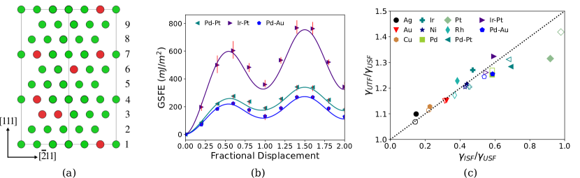
Figure 8: (a) Supercell for GSFE calculation of alloys; numbers adjacent to the atomic planes represent the layer number. (b) GSFE curves for Pd_0.75Pt_0.25, Ir_0.75Pt_0.25, and Pd_0.75Au_0.25 alloys. The symbols are from DFT calculations, while the curves are generated from Equation 2, using $\gamma_{ISF}$, $\gamma_{ESF}$, and $G$ values predicted via ML. (c) $\gamma_{UTF}/\gamma_{USF}$ scales linearly with $\gamma_{ISF}/\gamma_{USF}$, as shown by the dotted line. Comparison of actual values from DFT calculations (solid symbols) and predicted values (open symbols).

So far, we have focused on training ML models for predicting $\gamma_{ISF},\gamma_{ESF}$ and $G$. Finally, we take up the most challenging task of predicting the entire GSFE. Conventionally, one should calculate the GSFE curves for several alloys using DFT and use them to train ML models. However, calculating the GSFE curves for alloys is computationally very expensive. Instead, we use the predicted $G$, $\gamma_{ISF}$ and $\gamma_{ESF}$ values from the previous section and construct the GSFE curves using Equation 2. For a binary alloy, we use the rule of mixture to get the value of $c$ (listed after Equation 2), which is the weighted average of the pure element’s values. The following discussion shows that our method makes GSFE prediction 80X faster for alloys.

Figure 8 compares the predicted GSFE curves with actual DFT values, illustrated for binary Pd-Pt, Ir-Pt, and Pd-Au alloys. We use the same technique as described earlier (Figure 2), but with a nine times larger supercell, having cell vectors $\frac{3}{2}[\overline{1}10],\frac{3}{2}[\overline{1}01],[111]$. Such a supercell contains eighty-one atoms, nine each in 9 different layers [Figure 8(a)]. We generate SQS to describe the random arrangement of constituent atoms in a binary alloy and use a k-point mesh of $9\times 9\times 3$. Because of the randomness, each layer has a different composition [Figure 8(a)], and the GSFE curve depends on the specific choice of layers during the deformation. For example, we start by fixing layer 1 and displacing layers 2 to 9, followed by fixing layers 1-2 and displacing layers 3 to 9, etc., as shown in Figure 8(a). Thus, we have to repeat the calculation eight times, and the average value yields one single DFT data point on a GSFE curve [Figure 8(b)]. The error bars show the lowest and highest among the eight DFT values calculated. Since there are 10 data points on a GSFE curve, we need to perform 80 calculations to get the entire GSFE curve from DFT directly.

Considering the large number of atoms in the supercell, predicting GSFE directly from DFT is computationally expensive for alloys. As an alternative, the proposed ML approach requires only one DFT calculation to get the DOS and compute relevant parameters like $\varepsilon_{d},W_{d},z_{d},z_{s}$, and $r_{0}$. Using these parameters, one can predict $\gamma_{ISF},\gamma_{ESF}$, and $G$ using the ML model and finally predict the GSFE curve using Equation 2. Figure 8(b) illustrates that the ML-predicted GSFE curves are in good agreement with the actual DFT points (based on eighty DFT calculations). As shown in Figure 8(c), $\gamma_{UTF}/\gamma_{USF}$ scales linearly with $\gamma_{ISF}/\gamma_{USF}$. Predicted values agree reasonably well with the DFT results.

IV Conclusions

In conclusion, we have proposed a combined ab initio and ML-based model that can accelerate the computational prediction of GSFE curves for alloys by a factor of 80. The training dataset is generated using DFT calculations to find the SFE values of 106 metals and alloys using the ANNNI model. The features used for training the ML algorithms come from the physics-based Friedel model. The features are obtained from the electronic DOS, calculated using DFT. Other than accelerating the process of GSFE calculation, the present work also highlights a deep connection between the physics of d-electrons and the deformation behavior of transition metals and alloys. Our study reveals a highly non-linear dependence of shear modulus and stacking fault energies on the electronic features, which requires a combined approach involving state-of-the-art ab initio calculations and machine learning methods for complete understanding. The present model can accelerate alloy designing with targeted mechanical behavior by providing a fast method of screening materials in terms of stacking fault energies.

V Acknowledgements

We acknowledge National Super Computing Mission (NSM) for providing computing resources of “PARAM Sanganak” at IIT Kanpur, which is implemented by CDAC and supported by the Ministry of Electronics and Information Technology (MeitY) and Department of Science and Technology (DST), Government of India. We also thank ICME National Hub, IIT Kanpur and CC, IIT Kanpur for providing HPC facility.

References

- Molnár et al. [2019] D. Molnár, X. Sun, S. Lu, W. Li, G. Engberg, and L. Vitos, Effect of temperature on the stacking fault energy and deformation behaviour in 316l austenitic stainless steel, Materials Science and Engineering: A 759, 490 (2019)
- Zhang et al. [2018] X. Zhang, B. Grabowski, F. Körmann, A. V. Ruban, Y. Gong, R. C. Reed, T. Hickel, and J. Neugebauer, Temperature dependence of the stacking-fault gibbs energy for al, cu, and ni, Phys. Rev. B 98, 224106 (2018)
- Andric et al. [2019] P. Andric, B. Yin, and W. Curtin, Stress-dependence of generalized stacking fault energies, Journal of the Mechanics and Physics of Solids 122, 262 (2019)
- Linda et al. [2022] A. Linda, P. K. Tripathi, S. Nagar, and S. Bhowmick, Effect of pressure on stacking fault energy and deformation behavior of face-centered cubic metals, Materialia 26, 101598 (2022)
- Shao et al. [2017] Q. Shao, L. Liu, T. Fan, D. Yuan, and J. Chen, Effects of solute concentration on the stacking fault energy in copper alloys at finite temperatures, Journal of Alloys and Compounds 726, 601 (2017)
- Kumar et al. [2023] J. Kumar, A. Linda, M. Sadhasivam, K. Pradeep, N. Gurao, and K. Biswas, The effect of si addition on the structure and mechanical properties of equiatomic cocrfemnni high entropy alloy by experiment and simulation, Materialia 27, 101707 (2023)
- Zhang et al. [2019] Y. Zhang, J. Guo, J. Chen, C. Wu, K. S. Kormout, P. Ghosh, and Z. Zhang, On the stacking fault energy related deformation mechanism of nanocrystalline cu and cu alloys: A first-principles and tem study, Journal of Alloys and Compounds 776, 807 (2019)
- Zhao et al. [2017] S. Zhao, G. M. Stocks, and Y. Zhang, Stacking fault energies of face-centered cubic concentrated solid solution alloys, Acta Materialia 134, 334 (2017)
- Li et al. [2023] L. Li, Z. Zhang, P. Zhang, and Z. Zhang, A review on the fatigue cracking of twin boundaries: Crystallographic orientation and stacking fault energy, Progress in Materials Science 131, 101011 (2023)
- Su et al. [2021] R. Su, D. Neffati, Y. Zhang, J. Cho, J. Li, H. Wang, Y. Kulkarni, and X. Zhang, The influence of stacking faults on mechanical behavior of advanced materials, Materials Science and Engineering: A 803, 140696 (2021)
- An et al. [2019] X. An, S. Wu, Z. Wang, and Z. Zhang, Significance of stacking fault energy in bulk nanostructured materials: Insights from cu and its binary alloys as model systems, Progress in Materials Science 101, 1 (2019)
- Tian et al. [2014] C. Tian, G. Han, C. Cui, and X. Sun, Effects of stacking fault energy on the creep behaviors of ni-base superalloy, Materials & Design 64, 316 (2014)
- Delavignette and Amelinckx [1962] P. Delavignette and S. Amelinckx, Dislocation patterns in graphite, Journal of Nuclear Materials 5, 17 (1962)
- Werner et al. [2021] K. V. Werner, F. Niessen, M. Villa, and M. A. J. Somers, Experimental validation of negative stacking fault energies in metastable face-centered cubic materials, Applied Physics Letters 119, 141902 (2021)
- Rafaja et al. [2014] D. Rafaja, C. Krbetschek, C. Ullrich, and S. Martin, Stacking fault energy in austenitic steels determined by using in situ X-ray diffraction during bending, Journal of Applied Crystallography 47, 936 (2014)
- Byun [2003] T. Byun, On the stress dependence of partial dislocation separation and deformation microstructure in austenitic stainless steels, Acta Materialia 51, 3063 (2003)
- Su et al. [2019] Y. Su, S. Xu, and I. J. Beyerlein, Density functional theory calculations of generalized stacking fault energy surfaces for eight face-centered cubic transition metals, Journal of Applied Physics 126, 105112 (2019)
- Hunter et al. [2014] A. Hunter, R. F. Zhang, and I. J. Beyerlein, The core structure of dislocations and their relationship to the material -surface, Journal of Applied Physics 115, 134314 (2014)
- Hu and Yang [2013] Q.-M. Hu and R. Yang, Basal-plane stacking fault energy of hexagonal close-packed metals based on the ising model, Acta Materialia 61, 1136 (2013)
- Wu et al. [2010] X.-Z. Wu, R. Wang, S.-F. Wang, and Q.-Y. Wei, Ab initio calculations of generalized-stacking-fault energy surfaces and surface energies for fcc metals, Applied Surface Science 256, 6345 (2010)
- Jarlöv et al. [2022] A. Jarlöv, W. Ji, Z. Zhu, Y. Tian, R. Babicheva, R. An, H. L. Seet, M. L. S. Nai, and K. Zhou, Molecular dynamics study on the strengthening mechanisms of cr–fe–co–ni high-entropy alloys based on the generalized stacking fault energy, Journal of Alloys and Compounds 905, 164137 (2022)
- Joós et al. [1994] B. Joós, Q. Ren, and M. S. Duesbery, Peierls-nabarro model of dislocations in silicon with generalized stacking-fault restoring forces, Phys. Rev. B 50, 5890 (1994)
- Hartford et al. [1998] J. Hartford, B. von Sydow, G. Wahnström, and B. I. Lundqvist, Peierls barriers and stresses for edge dislocations in pd and al calculated from first principles, Phys. Rev. B 58, 2487 (1998)
- Shang et al. [2012a] S. L. Shang, W. Y. Wang, Y. Wang, Y. Du, J. X. Zhang, A. D. Patel, and Z. K. Liu, Temperature-dependent ideal strength and stacking fault energy of fcc ni: a first-principles study of shear deformation, Journal of Physics: Condensed Matter 24, 155402 (2012a)
- Shang et al. [2012b] S. L. Shang, C. L. Zacherl, H. Z. Fang, Y. Wang, Y. Du, and Z. K. Liu, Effects of alloying element and temperature on the stacking fault energies of dilute ni-base superalloys, Journal of Physics: Condensed Matter 24, 505403 (2012b)
- El Kadiri et al. [2013] H. El Kadiri, J. Kapil, A. Oppedal, L. Hector, S. R. Agnew, M. Cherkaoui, and S. Vogel, The effect of twin–twin interactions on the nucleation and propagation of 101¯2 twinning in magnesium, Acta Materialia 61, 3549 (2013)
- Linda et al. [2024] A. Linda, M. F. Akhtar, and S. Bhowmick, Deformation in metals: Insights from ab-initio calculations, in Proceedings of the International Conference on Metallurgical Engineering and Centenary Celebration, edited by S. Patra, S. Sinha, G. S. Mahobia, and D. Kamble (Springer Nature Singapore, Singapore, 2024) pp. 83–92
- Kamimura et al. [2018] Y. Kamimura, K. Edagawa, A. Iskandarov, M. Osawa, Y. Umeno, and S. Takeuchi, Peierls stresses estimated via the peierls-nabarro model using ab-initio -surface and their comparison with experiments, Acta Materialia 148, 355 (2018)
- Xu et al. [2020] S. Xu, J. R. Mianroodi, A. Hunter, B. Svendsen, and I. J. Beyerlein, Comparative modeling of the disregistry and peierls stress for dissociated edge and screw dislocations in al, International Journal of Plasticity 129, 102689 (2020)
- Ma et al. [2022] T. Ma, H. Kim, N. Mathew, D. J. Luscher, L. Cao, and A. Hunter, Dislocation transmission across 3112 incoherent twin boundary: a combined atomistic and phase-field study, Acta Materialia 223, 117447 (2022)
- Schönecker et al. [2021] S. Schönecker, W. Li, L. Vitos, and X. Li, Effect of strain on generalized stacking fault energies and plastic deformation modes in fcc-hcp polymorphic high-entropy alloys: A first-principles investigation, Phys. Rev. Mater. 5, 075004 (2021)
- Zhu and Wu [2023] L. Zhu and Z. Wu, Effects of short range ordering on the generalized stacking fault energy and deformation mechanisms in fcc multiprincipal element alloys, Acta Materialia 259, 119230 (2023)
- Yang et al. [2023] C. Yang, B. Zhang, L. Fu, Z. Wang, J. Teng, R. Shao, Z. Wu, X. Chang, J. Ding, L. Wang, and X. Han, Chemical inhomogeneity–induced profuse nanotwinning and phase transformation in aucu nanowires, Nature Communications 14, 5705 (2023)
- Wen et al. [2022] D. Wen, B. Kong, S. Wang, L. Liu, Q. Song, and Z. Yin, Mechanism of stress- and thermal-induced fct → hcp → fcc crystal structure change in a tial-based alloy compressed at elevated temperature, Materials Science and Engineering: A 840, 143011 (2022)
- Pei et al. [2021] Z. Pei, B. Dutta, F. Körmann, and M. Chen, Hidden effects of negative stacking fault energies in complex concentrated alloys, Phys. Rev. Lett. 126, 255502 (2021)
- Werner et al. [2023] K. V. Werner, F. Niessen, W. Li, S. Lu, L. Vitos, M. Villa, and M. A. Somers, Reconciling experimental and theoretical stacking fault energies in face-centered cubic materials with the experimental twinning stress, Materialia 27, 101708 (2023)
- You et al. [2023] D. You, O. K. Celebi, A. S. K. Mohammed, and H. Sehitoglu, Negative stacking fault energy in fcc materials-its implications, International Journal of Plasticity 170, 103770 (2023)
- Wei and Tasan [2020] S. Wei and C. C. Tasan, Deformation faulting in a metastable cocrniw complex concentrated alloy: A case of negative intrinsic stacking fault energy?, Acta Materialia 200, 992 (2020)
- Shih et al. [2021] M. Shih, J. Miao, M. Mills, and M. Ghazisaeidi, Stacking fault energy in concentrated alloys, Nature Communications 12, 3590 (2021)
- Walter et al. [2020] M. Walter, L. Mujica Roncery, S. Weber, L. Leich, and W. Theisen, Xrd measurement of stacking fault energy of cr–ni austenitic steels: influence of temperature and alloying elements, Journal of Materials Science 55, 13424 (2020)
- Chandan et al. [2021] A. Chandan, S. Tripathy, B. Sen, M. Ghosh, and S. Ghosh Chowdhury, Temperature dependent deformation behavior and stacking fault energy of fe40mn40co10cr10 alloy, Scripta Materialia 199, 113891 (2021)
- Sun et al. [2021] X. Sun, S. Lu, R. Xie, X. An, W. Li, T. Zhang, C. Liang, X. Ding, Y. Wang, H. Zhang, and L. Vitos, Can experiment determine the stacking fault energy of metastable alloys?, Materials & Design 199, 109396 (2021)
- Hu et al. [2016] H. Hu, M. Zhao, X. Wu, Z. Jia, R. Wang, W. Li, and Q. Liu, The structural stability, mechanical properties and stacking fault energy of al3zr precipitates in al-cu-zr alloys: Hrtem observations and first-principles calculations, Journal of Alloys and Compounds 681, 96 (2016)
- Shi et al. [2018] S. Shi, L. Zhu, H. Zhang, Z. Sun, and R. Ahuja, Mapping the relationship among composition, stacking fault energy and ductility in nb alloys: A first-principles study, Acta Materialia 144, 853 (2018)
- Stange et al. [2015] H. Stange, S. Brunken, H. Hempel, H. Rodriguez-Alvarez, N. Schäfer, D. Greiner, A. Scheu, J. Lauche, C. A. Kaufmann, T. Unold, D. Abou-Ras, and R. Mainz, Effect of Na presence during CuInSe2 growth on stacking fault annihilation and electronic properties, Applied Physics Letters 107, 152103 (2015)
- Wang et al. [2014] W. Y. Wang, S. L. Shang, Y. Wang, Z.-G. Mei, K. A. Darling, L. J. Kecskes, S. N. Mathaudhu, X. D. Hui, and Z.-K. Liu, Effects of alloying elements on stacking fault energies and electronic structures of binary mg alloys: A first-principles study, Materials Research Letters 2, 29 (2014)
- Li et al. [2022] X. Li, S. Schönecker, L. Vitos, and X. Li, Generalized stacking faults energies of face-centered cubic high-entropy alloys: A first-principles study, Intermetallics 145, 107556 (2022)
- Qi and Mishra [2007] Y. Qi and R. K. Mishra, Ab initio study of the effect of solute atoms on the stacking fault energy in aluminum, Phys. Rev. B 75, 224105 (2007)
- Natarajan and Van der Ven [2020] A. R. Natarajan and A. Van der Ven, Linking electronic structure calculations to generalized stacking fault energies in multicomponent alloys, npj Computational Materials 6, 80 (2020)
- Harris et al. [1966] I. Harris, I. Dillamore, R. Smallman, and B. Beeston, The influence of d-band structure on stacking-fault energy, Philosophical magazine 14, 325 (1966)
- Datta et al. [2008] A. Datta, U. Waghmare, and U. Ramamurty, Structure and stacking faults in layered mg–zn–y alloys: A first-principles study, Acta Materialia 56, 2531 (2008)
- Kumar et al. [2018] K. Kumar, R. Sankarasubramanian, and U. V. Waghmare, Influence of dilute solute substitutions in ni on its generalized stacking fault energies and ductility, Computational Materials Science 150, 424 (2018)
- Shen et al. [2020] Y. Shen, H. Wang, and Q. An, Modified generalized stacking fault energy surface of ii–vi ionic crystals from excess electrons and holes, ACS Applied Electronic Materials 2, 56 (2020)
- Li et al. [2015] Z. Li, J. R. Kermode, and A. De Vita, Molecular dynamics with on-the-fly machine learning of quantum-mechanical forces, Phys. Rev. Lett. 114, 096405 (2015)
- Ahmad et al. [2023] O. Ahmad, N. Kumar, R. Mukherjee, and S. Bhowmick, Accelerating microstructure modeling via machine learning: A method combining autoencoder and convlstm, Phys. Rev. Mater. 7, 083802 (2023)
- Schütt et al. [2014] K. T. Schütt, H. Glawe, F. Brockherde, A. Sanna, K. R. Müller, and E. K. U. Gross, How to represent crystal structures for machine learning: Towards fast prediction of electronic properties, Phys. Rev. B 89, 205118 (2014)
- Zhang et al. [2020] H. Zhang, H. Fu, X. He, C. Wang, L. Jiang, L.-Q. Chen, and J. Xie, Dramatically enhanced combination of ultimate tensile strength and electric conductivity of alloys via machine learning screening, Acta Materialia 200, 803 (2020)
- Liu et al. [2020] X. Liu, X. Li, Q. He, D. Liang, Z. Zhou, J. Ma, Y. Yang, and J. Shen, Machine learning-based glass formation prediction in multicomponent alloys, Acta Materialia 201, 182 (2020)
- Krishna et al. [2021] Y. V. Krishna, U. K. Jaiswal, and R. M. R, Machine learning approach to predict new multiphase high entropy alloys, Scripta Materialia 197, 113804 (2021)
- Revi et al. [2021] V. Revi, S. Kasodariya, A. Talapatra, G. Pilania, and A. Alankar, Machine learning elastic constants of multi-component alloys, Computational Materials Science 198, 110671 (2021)
- Chong et al. [2021] X. Chong, S.-L. Shang, A. M. Krajewski, J. D. Shimanek, W. Du, Y. Wang, J. Feng, D. Shin, A. M. Beese, and Z.-K. Liu, Correlation analysis of materials properties by machine learning: illustrated with stacking fault energy from first-principles calculations in dilute fcc-based alloys, Journal of Physics: Condensed Matter 33, 295702 (2021)
- Mahato et al. [2024] S. Mahato, N. P. Gurao, and K. Biswas, Accelerated prediction of stacking fault energy in fcc medium entropy alloys using multilayer perceptron neural networks: correlation and feature analysis, Modelling and Simulation in Materials Science and Engineering 32, 035021 (2024)
- Liu et al. [2023] X. Liu, Y. Zhu, C. Wang, K. Han, L. Zhao, S. Liang, M. Huang, and Z. Li, A statistics-based study and machine-learning of stacking fault energies in heas, Journal of Alloys and Compounds 966, 171547 (2023)
- Hu et al. [2021] Y.-J. Hu, A. Sundar, S. Ogata, and L. Qi, Screening of generalized stacking fault energies, surface energies and intrinsic ductile potency of refractory multicomponent alloys, Acta Materialia 210, 116800 (2021)
- Wang et al. [2021a] M. Wang, H. Yu, Y. Chen, and M. Huang, Machine learning assisted screening of non-rare-earth elements for mg alloys with low stacking fault energy, Computational Materials Science 196, 110544 (2021a)
- Khan et al. [2022] T. Z. Khan, T. Kirk, G. Vazquez, P. Singh, A. Smirnov, D. D. Johnson, K. Youssef, and R. Arróyave, Towards stacking fault energy engineering in fcc high entropy alloys, Acta Materialia 224, 117472 (2022)
- Arora et al. [2022a] G. Arora, A. Manzoor, and D. S. Aidhy, Charge-density based evaluation and prediction of stacking fault energies in Ni alloys from DFT and machine learning, Journal of Applied Physics 132, 225104 (2022a)
- Arora et al. [2022b] G. Arora, S. Kamrava, P. Tahmasebi, and D. S. Aidhy, Charge-density based convolutional neural networks for stacking fault energy prediction in concentrated alloys, Materialia 26, 101620 (2022b)
- Kresse and Joubert [1999] G. Kresse and D. Joubert, From ultrasoft pseudopotentials to the projector augmented-wave method, Phys. Rev. B 59, 1758 (1999)
- Kresse and Furthmüller [1996] G. Kresse and J. Furthmüller, Efficient iterative schemes for ab-initio total energy calculations using a plane-wave basis set, Phys. Rev. B 54, 11169 (1996)
- Perdew et al. [1996] J. P. Perdew, K. Burke, and M. Ernzerhof, Generalized gradient approximation made simple, Phys. Rev. Lett. 77, 3865 (1996)
- Dillamore and Smallman [1965] I. L. Dillamore and R. E. Smallman, The stacking-fault energy of f.c.c. metals, The Philosophical Magazine: A Journal of Theoretical Experimental and Applied Physics 12, 191 (1965)
- Gallagher [1970] P. C. J. Gallagher, The influence of alloying, temperature, and related effects on the stacking fault energy, Metallurgical Transactions 1, 2429 (1970)
- Hirth et al. [1983] J. P. Hirth, J. Lothe, and T. Mura, Theory of Dislocations (2nd ed.), Journal of Applied Mechanics 50, 476 (1983)
- Buch [2005] A. Buch, Short handbook of metal elements properties and elastic properties of pure metals, 3rd ed. (Krzysztof Biesaga, 2005)
- Kibey et al. [2007] S. Kibey, J. B. Liu, D. D. Johnson, and H. Sehitoglu, Energy pathways and directionality in deformation twinning, Applied Physics Letters 91, 181916 (2007)
- Le Page and Saxe [2001] Y. Le Page and P. Saxe, Symmetry-general least-squares extraction of elastic coefficients from ab initio total energy calculations, Phys. Rev. B 63, 174103 (2001)
- Wang et al. [2021b] V. Wang, N. Xu, J.-C. Liu, G. Tang, and W.-T. Geng, Vaspkit: A user-friendly interface facilitating high-throughput computing and analysis using vasp code, Computer Physics Communications 267, 108033 (2021b)
- [79] See supplemental material for technical details of shear modulus calculation, materials parameters calculated from density functional theory, gaussian process regression, support vector regression, and feature importance analysis., URLwillbeinsertedbypublisher.
- Harrison [2012] W. A. Harrison, Electronic structure and the properties of solids: the physics of the chemical bond (Courier Corporation, 2012)
- van de Walle et al. [2013] A. van de Walle, P. Tiwary, M. de Jong, D. Olmsted, M. Asta, A. Dick, D. Shin, Y. Wang, L.-Q. Chen, and Z.-K. Liu, Efficient stochastic generation of special quasirandom structures, Calphad 42, 13 (2013)
- Schmidhuber [2015] J. Schmidhuber, Deep learning in neural networks: An overview, Neural Networks 61, 85 (2015)