Nonequilibrium entropy from density estimation

Abstract

Entropy is a central concept in physics, but can be challenging to calculate even for systems that are easily simulated. This is exacerbated out of equilibrium, where generally little is known about the distribution characterizing simulated configurations. However, modern machine learning algorithms can estimate the probability density characterizing an ensemble of images, given nothing more than sample images assumed to be drawn from this distribution. We show that by mapping system configurations to images, such approaches can be adapted to the efficient estimation of the density, and therefore the entropy, from simulated or experimental data. We then use this idea to obtain entropic limit cycles in a kinetic Ising model driven by an oscillating magnetic field. Despite being a global probe, we demonstrate that this allows us to identify and characterize stochastic dynamics at parameters near the dynamical phase transition.

Evaluating entropy of statistical mechanical systems from simulations or experimental snapshots is a challenge that has drawn attention repeatedly for more than half a century. In equilibrium, this issue was largely resolved by the introduction of celebrated and widely used concepts like thermodynamic integration [1] and later the Wang–Landau method [2]. On the other hand, entropy is of particular interest in nonequilibrium situations, where most state variables are ill-defined [3, 4]. Here, despite decades of study, the question of how entropy can be generically and efficiently evaluated has never been fully answered [5, 6, 7, 8, 9].

The problem is succinctly stated as follows. Suppose we can simulate the statistics of a system. In all that follows, simulating a system may be considered equivalent to experimentally realizing and fully characterizing it. The ability to simulate implies that we can access a set of $N$ sample configurations $\left\{\mathbf{x}_{i}\right\}$, with index $i\in\left\{1,\ldots,N\right\}$, drawn from some (unknown) probability distribution $P\left(\mathbf{x}\right)$ describing the system’s behavior at some moment in time. Given these samples, we can estimate expectation values of various properties of the system. For example, given the energy of a configuration $E\left(\mathbf{x}\right)$, the mean energy is

$$\left\langle E\right\rangle=\int\mathrm{d}\mathbf{x}P\left(\mathbf{x}\right)E\left(\mathbf{x}\right)=\sum_{i=1}^{N}\frac{E\left(\mathbf{x}_{i}\right)}{N}+O\left(\frac{1}{\sqrt{N}}\right).$$ (1)

Importantly, eq. (1) can be evaluated without knowing $P\left(\mathbf{x}\right)$. On the other hand, analogous considerations for the Von Neumann entropy (or similarly the free energy) give

$$\left\langle S\right\rangle =\frac{1}{N}\sum_{i=1}^{N}\ln\left[P\left(\mathbf{x}_{i}\right)\right]+O\left(\frac{1}{\sqrt{N}}\right),$$ (2)

and knowledge of $P\left(\mathbf{x}\right)$ is expressly required. In equilibrium, some progress can be made from knowing that $P\left(\mathbf{x}\right)\sim e^{-\frac{E\left(\mathbf{x}\right)}{k_{B}T}}$; but for generic nonequilibrium situations we have no a priori knowledge of the distribution.

Numerous routes around this have been proposed in the literature, from the beautiful early work of Ma on coincidence counting in 1981 [10] to increasingly sophisticated recent approaches based on compression algorithms [11, 4] and machine learning models for mutual information between subsystems [12]. Other approaches are approximate, for example relying on structure factors [13, 14] or making other assumptions [15]. Rapidly increasing interest in applying machine learning techniques to a variety of physical problems [16, 17, 18] makes many of these directions appealing. Despite these continuing advances, existing methodologies are either slow to converge in the number of samples; intrinsically biased; or too computationally expensive to be applied to large systems without additional assumptions.

Entropy from density estimation.

Here, we propose a surprisingly straightforward and efficient solution based on first solving a seemingly harder problem: density estimation. In machine learning terms, density estimation is the task of parametrizing an optimal probability distribution $P_{\boldsymbol{\vartheta}}\left(\mathbf{x}\right)$ from a set of samples $\mathbf{x}_{i}$ taken from an unknown distribution $P\left(\mathbf{x}\right)$; here $\boldsymbol{\vartheta}$ is a set of parameters. There is no unique criterion for what should be considered optimal, but a common approach is to select $\boldsymbol{\vartheta}$ so as to minimize the Kullback–Leibler divergence (KLD) between $P_{\boldsymbol{\vartheta}}\left(\mathbf{x}\right)$ and the prior distribution $P_{\mathrm{Prior}}\left(\mathbf{x}\right)\equiv\frac{1}{N}\sum_{i=1}^{N}\delta\left(\mathbf{x}-\mathbf{x}_{i}\right)$. Given a model distribution $P_{\boldsymbol{\vartheta}}\left(\mathbf{x}\right)$ and samples $\mathbf{x}_{i}$, eq. (2) can then be approximated by

$$\left\langle S\right\rangle\approx\frac{1}{N}\sum_{i=1}^{N}\ln\left(P_{\boldsymbol{\vartheta}}\left(\mathbf{x}_{i}\right)\right).$$ (3)

Perhaps the simplest density estimation algorithm is the division of space into bins and the construction of a normalized histogram. Another simple approach, known as kernel density estimation, involves convolving $P_{\mathrm{Prior}}\left(\mathbf{x}\right)$ with, e.g., a Gaussian function $P_{\boldsymbol{\vartheta}}\left(\mathbf{x}\right)={\displaystyle\frac{1}{\sqrt{2\pi\sigma^{2}N^{2}}}\sum_{i=1}^{N}e^{-\left(\frac{\mathbf{x}-\mathbf{x}_{i}}{4\sigma}\right)^{2}}}$. The lone parameter $\boldsymbol{\vartheta}=\sigma$ then expresses a trade-off between the smoothness and resolution of the resulting distribution. However, histograms and kernel methods do not scale well to high dimension. Recent interest in applying density estimation to extremely high-dimensional problems like image processing has resulted in a variety of novel and highly accurate generative models based on artificial neural networks [19, 20, 21, 22, 23, 24, 25, 26, 27, 28].

Generative models earn their name from their ability to generate samples drawn from the distribution they describe. In the context of statistical mechanics, this has been taken advantage of to not only characterize—but rather to effectively simulate—equilibrium models, by minimizing the variational free energy of generated samples [29, 30, 31, 32, 33]. This approach requires less ad hoc simulation and analysis than traditional approaches like Wang–Landau, but is much more expensive, and in practice it has only been used for small systems. In particular, ref. [30] solved a $24\times 24$ square Ising model, whereas ref. [12] reached $64\times 64$; for comparison, Wang and Landau demonstrated their approach on the $256\times 256$ case two decades earlier [2].

In what follows, we first demonstrate that by leveraging standard simulations to generate samples and using generative density estimation to learn the distribution, system sizes comparable with those treatable by the Wang–Landau algorithm become easily accessible. We then show that nonequilibrium systems become just as tractable, and use our approach to investigate the dynamics of entropy in a nonequilibrium Ising model driven by an oscillating magnetic field. There, we study the entropic limit cycle at the boundary between the ferromagnetic and paramagnetic phases, showing that it reveals a nonequilibrium critical regime with long-lived hysteretic behavior.

Autoregressive ansatz.

While the evaluation of entropy from density estimation is a completely general idea, it is useful to limit our attention to physical models for which configurations may be expressed as two dimensional images. To be concrete, we assume $\left(\mathbf{x}_{i}\right)^{nm}=\sigma_{i}^{nm}$, where $n\in\left\{1,2,\ldots,L_{1}\right\}$ and $m\in\left\{1,2,\ldots,L_{2}\right\}$ are spatial indices; $\sigma_{i}^{nm}$ can take on any of some discrete set of values; and $L_{1}$ and $L_{2}$ determine the system’s size. For example, in the Ising model on an $L\times L$ square lattice, $\sigma\in\left\{-1,1\right\}$ and $L_{1}=L_{2}=L$.

Given the assumptions above, we employ a highly successful approach to density estimation known as PixelCNN++ [34, 21, 23]. This is an autoregressive model, meaning that to make the joint distribution $P\left(\mathbf{x}\right)$ tractable, it is decomposed using the chain rule into a product of conditionals:

$$P_{\boldsymbol{\vartheta}_{1},\ldots,\boldsymbol{\vartheta}_{N}}\left(\mathbf{x}\right)=\prod_{\ell=1}^{N}P_{\boldsymbol{\vartheta}_{\ell}}\left(\left.x^{n_{\ell}m_{\ell}}\right|\left\{x^{n_{\ell^{\prime}}m_{\ell^{\prime}}},\ell^{\prime}<\ell\right\}\right).$$ (4)

Here, the indices $\ell$ and $\ell^{\prime}$ define a 1D ordering over the spatial indices $n$ and $m$ (i.e. over spins in an Ising model) and $N=L_{1}\cdot L_{2}$. The conditionals $P_{\boldsymbol{\vartheta}_{\ell}}$ themselves are expressed in terms of an efficient neural network ansatz that allows for their rapid training in parallel, and the set of spins on which each spin’s conditional depends is effectively limited to simplify training [23]. Despite its intrinsically 1D nature, it turns out that a sequential scan over lines in 2D images often works very well in describing the distributions of complicated ensembles [27].

Equilibrium Ising model.

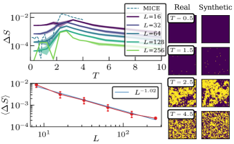
Figure 1: (upper left panel) Difference in entropy from exact result at different system sizes $L$, as a function of temperature $T$. For comparison, the dashed line is the $L=64$ MICE data from ref. [12]. (lower left panel) Temperature-averaged entropy difference, with standard deviation as error bars. (right panels) Monte Carlo samples at different temperature (left column), next to samples drawn from the generative ansatz at the same temperatures (right column).

We begin by benchmarking our approach against known results for the ferromagnetic Ising model on a square lattice with toroidal boundary conditions, given by

$$E\left(\mathbf{x}\right)=E\left(\boldsymbol{\sigma}\right)=-J\sum_{\left\langle nm,n^{\prime}m^{\prime}\right\rangle}\sigma^{nm}\sigma^{n^{\prime}m^{\prime}}+\underset{nm}{\sum}h\sigma^{nm},$$ (5)

where the sum in the first term is taken over nearest neighbors. Here, we set $J=1$ and employ it as our unit of energy. The system is simulated using a standard Monte Carlo procedure, with the Metropolis–Hastings algorithm[35] used at higher temperatures and the Wolff algorithm [36] used at critical and low temperatures. We generate 10,000 independent training samples and attempt to minimize a loss function comprising the KLD of $P_{\boldsymbol{\vartheta}_{1},\ldots,\boldsymbol{\vartheta}_{N}}\left(\mathbf{x}\right)$ with the prior. Training continues until the loss associated with 1,000 additional test samples reaches a plateau. A final set of samples is then used to estimate the entropy using Eq. (3), and a standard error is obtained from five independent calculations of this type.

The top left panel of Fig. 1 shows the error in our estimate for the entropy as a function of temperature, at several system sizes ranging from $L=16$ to $L=256$. Note that this is obtained from comparison with the exact result at finite system size [37], not with the thermodynamic limit [38]; other than statistical uncertainty, which is easily accounted for, this error is therefore entirely due to the bias introduced by the machine learning ansatz and its optimization, and is always positive. For comparison, we also reproduce the MICE result from Ref. [12] for $L=64$ (dashed line). The latter was obtained with 5,000 samples, but used data augmentation techniques to increase the effective number available.

We use the same number of samples for all system sizes, but each sample contains $L^{2}$ bits of information; therefore, more data was available at large system sizes, and as a result accuracy (generally) improves. On the other hand, one might expect larger systems to be harder to characterize—this, especially in the critical regime, where large length scales appear and errors are maximal. To gain some understanding of the method’s behavior, we plot the temperature-averaged entropy as a function of system size in the bottom left panel of Fig. 1. The overall trend is consistent with a power law, $\left\langle\Delta S\right\rangle\sim L^{-1.02}$. This is comparable with the ideal scaling for intrinsic quantities in Monte Carlo simulations, $\left\langle\Delta S\right\rangle\sim\frac{1}{\sqrt{L^{2}}}=L^{-1}$.

In the right panels, we show examples of real samples at several temperature regimes, alongside samples synthesized by the trained generative model at each temperature. The visual resemblance is striking, and it should be immediately clear that this generative capability promises to be a basis for powerful diagnostic techniques. In principle, the trained model could now be used to perform a simulation. However, since knowledge the distribution is sufficient information for evaluating any observable, it is difficult to imagine scenarios where enough samples are available to properly characterize the distribution, yet even more are still wanted for some other purpose. One intriguing and promising approach involves generation of systems that are too large to simulate [39, 40, 41], though it remains unknown whether this can capture, e.g., long-ranged correlations.

Kinetic Ising model and dynamical phases.

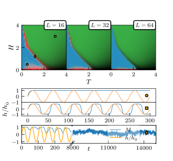
Figure 2: (top panels) Phases of the kinetic Ising model at different oscillating magnetic field amplitudes $H$ and temperatures $T$ and different system sizes $L$. The order parameters characterizing the dynamically ordered/ferromagnetic phase and the dynamically disordered/paramagnetic phase are marked in blue and green, respectively. The parameter for the strongly fluctuating/chaotic regime is marked in red (see text for details). (middle and bottom panels) Traces of the magnetization $\overline{M}$ at $L=16$ and in the three different regimes and averaged over 96 realizations, with symbols marking the parameters in the upper left panel.

Having established that modern density estimation techniques produce accurate estimates of entropy in equilibrium, we note that nothing in the method depends on taking samples from an equilibrium distribution. We therefore now consider a nonequilibrium application. In particular, we will explore the response of a 2D Ising ferromagnet to an oscillating magnetic field $H\left(t\right)=H\sin\left(\omega_{0}t\right)$, as described by Glauber dynamics [42], where every $L^{2}$ Metropolis steps are taken to be a time step. This is a minimal toy model for exploring hysteresis in magnetic systems [43, 44, 45], and is known to exhibit a dynamical phase transition [46, 47, 48, 49, 50, 51]. A dynamically disordered phase with zero period-averaged magnetization emerges at weak magnetic fields, small field frequencies and high temperatures; while a dynamically ordered phase with nonzero period-averaged magnetic response is observed elsewhere [52, 53].

The dynamical phase diagram at several system sizes is shown in the three top panels of Fig. 2, as a function of the temperature $T$ and magnetic field amplitude $H$, and with $\omega_{0}=\frac{2\pi}{50}$ throughout. To obtain this diagram, we plotted the order parameter $O_{\text{Ordered}}=\left|\left\langle\overline{M}\right\rangle\right|$, which characterizes the ordered phase, in blue (lower left regions); and the parameter $O_{\text{Disordered}}=\left\langle\left|\overline{M}\right|\right\rangle\left(1-O_{\text{Ordered}}\right)$, which characterizes the amplitude of oscillations in the disordered phase, in green (upper right regions). Here, $\left|\cdots\right|$ is the absolute value, $\overline{\cdots}$ is an ensemble average and $\left\langle\cdots\right\rangle$ is a time average over many cycles. Examples of the time dependence of the ensemble-averaged magnetization at $L=16$ in the ordered and disordered regimes, respectively, are shown in the two middle panels. Similar phase diagrams have appeared in the literature [50, 54], and the kink in the phase boundary at $H=2$ was found to result from the fact that the ordered regime actually comprises two dynamical phases with different nucleation dynamics [50].

Strong fluctuations at the phase boundary.

At certain parameters, both in and out of equilibrium, the Glauber dynamics of small systems are highly stochastic. In particular, they remain non-periodic for very long timescales even after averaging over an ensemble of 96 realizations (see bottom panel of Fig. 2 for an example). This behavior has been observed and discussed in the literature before [46, 50]. It can be characterized by the ensemble variance of the magnetization, $O_{\text{Fluctuating}}=\left\langle\overline{M^{2}}-\overline{M}^{2}\right\rangle$, which we plot in red in the top panels of Fig. 2.

Fluctuations of this kind are a mesoscopic effect: they become weaker and appear over smaller parameter regimes as the system size grows (i.e. going from leftmost to rightmost panel). Notably, $O_{\text{Fluctuating}}$ is large near equilibrium, at small magnetic fields and below the critical temperature (horizontal red strips at bottom of three top panels of Fig. 2). The hysteretic dynamics there can be approximately described as stochastic hopping between the two fully magnetized states, and is well understood [55, 56]. We will focus on the other manifold of parameters where large fluctuations appear: along the phase boundary (diagonal red strips in three top panels).

Signature of fluctuations in the entropic limit cycle.

The ensemble variance of magnetic fluctuations is easily accessible from simulations. However, it is generally more difficult to access experimentally than the mean magnetization: to obtain this, it would be necessary to perform, e.g., many local measurements in a large system, or many measurements of separate nanoscale crystals. Let us therefore consider an alternative: characterizing the critical strongly fluctuating regime using its entropy, e.g. by measuring the specific heat globally for an ensemble of many nanoscale samples (or uncorrelated regions in a large sample) at a series of temperatures. We will argue that this is sufficient, with one complication.

Since the system occupies a very small subset of its possible states in the near-equilibrium stochastic regime, we expect the entropy there to be almost as low as that of the equilibrium ferromagnet. In contrast, in the critical stochastic regime we expect the system to occupy a wide variety of states at any given moment, and therefore exhibit a high entropy compared to the ordered phase. On the other hand, the disordered phase is also high in entropy, so it is not immediately clear that these two scenarios can be distinguished from each other by entropy alone.

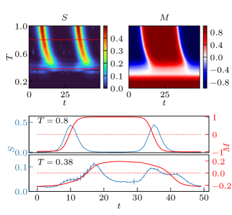
Figure 3: (top left) Entropic limit cycle for system size $L=32$, at magnetic field amplitude $H=2.5$. (top right) Magnetization limit cycle at same parameters. (Bottom panels) Constant temperature cuts across upper panels in the disordered (upper subpanel) and the critical strongly fluctuating (lower subpanel) regimes, at the red horizontal lines shown in top left panel.

We therefore propose to study the time dependence $\overline{S}\left(t\right)$ of the entropy within a limit cycle rather than its time-averaged value $\left\langle\overline{S}\right\rangle=\lim_{s\rightarrow\infty}\frac{\omega_{0}}{2\pi}\int_{s}^{s+\frac{2\pi}{\omega_{0}}}\mathrm{d}t\thinspace\overline{S}\left(t\right)$. Experimentally, this could be measured by performing a global specific heat measurement, but with heat injected by a sequence of short pulses with the same periodicity as the field. The quantity $\overline{S}\left(t\right)$, obtained from density estimation, is shown for the $L=32$ case in the top left panel of Fig. 3 at a range of temperatures spanning the transition. The corresponding limit cycle for the mean magnetization is shown in the top right panel. The two panels below show cuts across this data at two temperatures marked by horizontal red lines in the top left panel.

In the disordered phase, as might be expected, the entropy is large where the absolute value of the magnetization is small. As temperature is lowered the magnetic and entropic response gradually slow down and their peak shifts forward in time. At the other limit, where temperature is near zero, the system enters the ordered phase and entropy is negligible. Note that due to the constant initial phase of the field, at low temperature we break symmetry in favor of positive magnetization (see also the dynamics in the relevant panel of Fig. 2). This manifests itself in the red band at the bottom of the top right panel, and in the different magnitude of the two entropic peaks in the lower panel.

At temperatures near the phase transition (see cut in lower panel of Fig. 3), magnetic response is weaker, while entropic response is higher at all times. This directly demonstrates that the system achieves low magnetization by exploring states that are not fully magnetized, rather than by modifying the relative probability of occupying the two opposite fully magnetized states. The converse is true at lower temperatures (compare light red horizontal band in top right panel to the corresponding region in the top left panel). In that sense, the entropic limit cycle is a global measurement that provides the kind of information that would only otherwise be available in a local measurement (i.e. of the variance in the magnetization).

Conclusions.

We showed that generative density estimation algorithms are capable of accurately capturing the distributions characterizing certain statistical mechanical systems, with no input other than samples obtained by traditional simulation algorithms. After benchmarking the methodology on the equilibrium Ising model, we used it to investigate nonequilibrium physics in a kinetic Ising model. We obtained the time-dependent entropy of the system when driven by a periodic oscillating magnetic field. We found that global entropy can be used to demonstrate that near the dynamical phase transition, in a regime characterized by strong local fluctuations, the system attains a limit cycle where it is constantly exploring a large manifold of states.

Within machine learning frameworks, generative density estimation is straightforward to implement with a variety of algorithms. The method shown here is widely applicable, since it requires only that the system’s configuration can be (at least approximately) mapped onto a low-dimensional image. We’ve therefore provided a simple and freely available code repository demonstrating how to reproduce and extend our work [57].