SCALA: Split Federated Learning with Concatenated Activations
and Logit Adjustments
Abstract
Split Federated Learning (SFL) is a distributed machine learning framework which strategically divides the learning process between a server and clients and collaboratively trains a shared model by aggregating local models updated based on data from distributed clients. However, data heterogeneity and partial client participation result in label distribution skew, which severely degrades the learning performance. To address this issue, we propose SFL with Concatenated Activations and Logit Adjustments (SCALA). Specifically, the activations from the client-side models are concatenated as the input of the server-side model so as to centrally adjust label distribution across different clients, and logit adjustments of loss functions on both server-side and client-side models are performed to deal with the label distribution variation across different subsets of participating clients. Theoretical analysis and experimental results verify the superiority of the proposed SCALA on public datasets.
1 Introduction

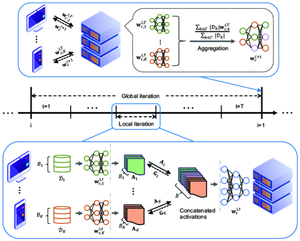
Split Federated Learning (SFL) (Jeon & Kim, 2020; Thapa et al., 2022; Gawali et al., 2021) is a promising technology that integrates the characteristics of both Federated Learning (FL) (Li et al., 2020a; McMahan et al., 2017) and Split Learning (SL) (Gupta & Raskar, 2018), where model splitting and aggregation are concurrently deployed, as depicted in Figure 1a. Specifically, akin to SL, SFL also splits the artificial intelligence (AI) model into two parts, with each part deployed separately on server and clients. In training phase, each client processes local data through the client-side model, and then sends the activations to server to complete the forward propagation. Then, the server updates the server-side model and sends back the backpropagated gradients to each client to finish the update of client-side model. In this way, clients only need to execute the initial layers of complex AI models like deep neural networks and offload the remaining layers to the server for execution. On the other hand, SFL employs parallel training to enhance training efficiency and utilizes FL technology to aggregate server-side and client-side models. Therefore, SFL takes the advantages of both FL and SL by combining the parallel training structure of FL and computation offloading of SL.
Same as other distributed machine learning methods, SFL also encounters the issue of skewed label distribution due to two-fold. The first is local label distribution skew (Zhang et al., 2022; Wang et al., 2021) caused by the data heterogeneity of clients where label distribution varies across clients. The second is global label distribution skew (Zhang et al., 2023a) brought by partial client participation, resulting in label distribution variation across different subsets of participating clients. Specifically, the local objective functions are inconsistent among clients due to local label distribution skew, causing the aggregated model to deviate from the global optimum (Wang et al., 2020; Woodworth et al., 2020; Acar et al., 2021). On the other hand, partial client participation (Yang et al., 2021a) is usually assumed, where only a subset of clients are involved in model training due to heterogenous communication and computational capabilities of clients. However, in this case the server can not access label distribution of non-participating clients, which is likely to exhibit a skewed label distribution and fails to learn a global model that can generalize well for all clients.
The common approaches to skewed label distribution are regularization (Li et al., 2020b; Shi et al., 2023; Chen et al., 2023), loss function calibration (Lee et al., 2022; Zhang et al., 2022), and client selection (Zhang et al., 2023a; Yang et al., 2021b). However, if the local label distribution is highly skewed, there are missing classes in the local data and the local model still exhibits adverse bias towards the existing labels. Moreover, the adverse bias is present in every layer of the model and intensifies as the depth of the model increases, and thus the classifier is the most severely affected (Luo et al., 2021). This issue is unavoidable in the distributed machine learning algorithms, where each client may lack certain classes of its local data.
To address the above issue of skewed label distribution, we propose SCALA whose core idea is to centrally adjust label information from clients at the server. On one hand, to deal with the local label distribution skew raised from data heterogeneity, as shown in Figure 1b, we concatenate the activations (output of the client-side models) to serve as input for the server-side model (i.e., the parallel SL step). This enables the server to train the server-side model centrally based on a dataset with concatenated label distribution, thereby effectively alleviating the bias introduced by local label distribution skew with missing classes. Concurrently, the clients share the same server-side model during training, directly addressing the deep-layer adverse bias as demonstrated in prior studies (Luo et al., 2021; Shang et al., 2022).
On the other hand, we adopt logit adjustment to tackle the global label distribution skew due to partial client participation. Note that the skewed label distribution in centralized training shows as a long-tail distribution (Menon et al., 2021; Zhong et al., 2021; Zhang et al., 2023b), where common loss functions may not be applicable. Specifically, the misclassification error of loss functions is related to label distribution, where high-frequency labels result in a smaller misclassification error, leading the model to focus on improving predictive accuracy for high-frequency labels. Therefore, we perform logit adjustments for both server-side and client-side models to mitigate the impact of label distribution on loss function updates. In detail, we employ logit adjustment to decrease the logits for high-frequency labels by a larger value and for low-frequency labels by a smaller value, thereby achieving a calibrated misclassification error that is independent of label distribution. Our main contributions are summarized as follows.
-
•
We propose a concatenated activations enabled SFL framework to address the issue of highly skewed local label distribution with missing classes, where the server-side model is trained in a centralized manner based on the concatenated activations output by participating clients.
-
•
We introduce the loss functions with logit adjustments for both the server-side and client-side models to address the issue of global label distribution skew, where logits before softmax cross-entropy is adjusted according to the concatenated label distribution and the local label distributions.
-
•
Several useful insights are obtained via our analysis: First, label distribution skew results in classifier bias, since it neglects the prediction of low-frequency labels and outputs higher accuracy for high-frequency labels. Second, logit adjustment can update the classifier without bias by enhancing the recognition of low-frequency labels at the cost of sacrificing the recognition for high-frequency labels.
2 Related Works
Split Federated Learning: SFL (Thapa et al., 2022) represents a significant advancement in distributed machine learning by combining the strengths of FL (McMahan et al., 2017) and SL (Gupta & Raskar, 2018). Recent researches focus on improving the communication efficiency of SFL. For example, (Wang et al., 2022; Wu et al., 2023) employ compression techniques to reduce the data volume of activations, while (Han et al., 2021) introduces an auxiliary network on the client side so that the server does not need to send gradients. Additionally, (Xiao et al., 2022; Thapa et al., 2022) propose privacy-preserving mechanisms for SFL, leveraging mixing activations and differential privacy to prevent the raw data from being reconstructed from the activations.
Long-tail Distribution: Long-tail distribution of data has gained significant traction due to its prevalence in real-world datasets (Zhong et al., 2021; Zhang et al., 2023b). Long-tailed data poses a challenge for traditional machine learning algorithms which often assume a balanced data distribution. Re-sampling and re-weighting are two commonly employed methods to address this issue. Re-sampling (Chawla et al., 2002) often involve either oversampling the minority classes or undersampling the majority classes to create a more balanced distribution. Re-weighting (Cao et al., 2019; Jamal et al., 2020), on the other hand, aims to adjust the contribution of each class during model training by assigning different weights to classes. Additionally, (Menon et al., 2021) defines a balanced class-probability function from a statistical perspective and proposes a logit adjustment algorithm. Representation learning and classifier training are decoupled in (Kang et al., 2020) to achieve strong long-tailed recognition ability.
Label Distribution Skew: Label distribution skew is a prevalent issue in distributed machine learning. On one hand, the variance in label distribution across clients leads to local label distribution skew. Recent works address this issue through optimizations on both the client and server sides. Specifically, (Li et al., 2020b; Tan et al., 2022; Shi et al., 2023; Chen et al., 2023; Mu et al., 2023) add extra regularization terms to the local loss function to reduce bias between local and global models. (Lee et al., 2022; Zhang et al., 2022) directly calibrate the local loss function based on the characteristics of local data to produce higher quality local models. Additionally, global classifiers are calibrated at the server side using virtual representations in (Luo et al., 2021; Shang et al., 2022) and the prioritization of high-quality client data at the server side is explored in (Ren et al., 2020; Fu et al., 2023; Yang et al., 2023; Nguyen et al., 2020; Michieli et al., 2022). For partial client participation, the varying subsets of participating clients lead to global label distribution skew, where the global label distribution shows as a long-tailed distribution. Recent works (Zhang et al., 2023a; Yang et al., 2021b) employ client selection to choose a balanced subset of participating clients to address this issue.
In this paper, we propose SCALA to fill the gap in the capabilities of SFL for dealing with label distribution skew. SCALA trains the server-side model with concatenated activations to addresses the unavoidable inconsistencies between local and global models (Li et al., 2020b; Lee et al., 2022; Zhang et al., 2022), particularly when local models are trained on data with missing classes. Moreover, for global label distribution skew, previous approaches (Zhang et al., 2023a; Yang et al., 2021b) adopt client selection, but we introduce logit adjustments to calibrate the loss functions directly, thereby mitigating the adverse effects of long-tail distributions.
Note that the proposed SCALA only requires the label information from participating clients. Compared to vanilla SL, it does not expose any additional client-side information. Additionally, existing communication-efficient solutions designed for SFL can also be applied to SCALA with the consideration of resource-constrained clients, which is however out of the scope of this paper.
3 Proposed Method: SCALA
In this section, we first describe the concatenated activations enabled SFL framework, followed by proposing the loss functions with logit adjustments for the server-side and client-side models.
3.1 Concatenated Activations Enabled SFL Framework
3.1.1 Preliminaries
We consider clients participating in the training indexed by , each holding local data of size . The goal of the clients is to learn a global model with the help of the server. In SFL, the global model is split into the client-side model , which is collaboratively trained and updated by the clients and the server, and the server-side model , which is only stored and trained on the server. The global model is obtained by minimizing the averaged loss over all participating clients as
| (1) |
where denotes the local expected loss function, and it is unbiasedly estimated by the empirical loss , i.e., . In addition, under the setting of model splitting, the empirical loss of client is formulated as
| (2) |
where is the client-side function mapping the input data to the activation space and is the server-side function mapping the activation to a scalar loss value.
3.1.2 Algorithm Description
As shown in Figure 2, we propose a concatenated activations enabled SFL framework. The server-side model is updated based on the concatenated activations, which we refer to as the parallel SL phase. And the client-side model is updated through aggregation, which we refer to as the FL phase. The pseudo-code is illustrated in Algorithm 1. At the start of training, the server will set the minibatch size , the number of local iterations indexed by , and the number of global iterations indexed by . Given a set of clients , concatenated activations enabled SFL will output a global model after global iterations. Taking the -th global iteration as an example, we provide a detailed description of the training process in the following, where the superscript is omitted for notational brevity.
Client-side models deployments (line 5-7). At the beginning of a global iteration, the server randomly selects a subset of clients and sets the minibatch size for each client in proportion to its local data size as
| (3) |
so that the number of local iterations can be synchronized. Then each client downloads the client-side model and the minibatch size from the server.
Parallel SL phase (line 8-20). The selected clients and the server collaborate to perform parallel SL over local iterations, during which the server-side model is updated at each local iteration. It is worth noting that the server-side model is updated at each local iteration in SCALA, whereas that is updated at each global iteration, i.e., at the -th local iteration, in traditional SFL. The detailed description of the process is as follows:
-
•
Step 1 (Forward propagation of client-side model): Each client randomly selects a minibatch of size as , where the sample set of the minibatch is denoted by and the label set of the minibatch is denoted by . Then each client performs forward propagation based on and computes the activations of the last layer of the client-side model as
(4) Then the activation and the label set are uploaded to the server.
-
•
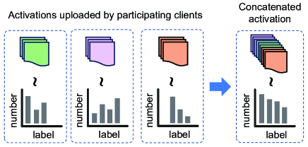
Step 2 (Backpropagation and update of server-side model): As shown in Figure 3, the server receives the activation sets from the selected clients and concatenates them as
(5) The corresponding labels for the activations are also concatenated as
(6) We can observed that the phenomenon of missing classes is mitigated, indicating an improvement in the local label distribution skew. Then, the server performs forward propagation for the concatenated activation , and updates the server-side model as
(7) where is the learning rate. Additionally, the server computes the backpropagated gradients as
(8) which is then sent back to each client .
- •
FL phase (line 21-24). After local iterations, each client uploads the client-side model to the server. Then the server aggregates the client-side models as
| (10) |
Note that all participating clients synchronously execute local iterations (line 9-13 and line 17-19), where the client-side models are updated locally and sent to the server for aggregation at the -th local iteration. The server-side model is centrally updated in each local iteration (line 14-15), where the input is concatenated from the activations uploaded by participating clients, thereby effectively mitigating the issue of missing classes under highly skewed local label distribution.
3.2 Logit Adjustments on Loss Functions
While the manner of concatenating activations offers a solution to the challenge of missing classes caused by local label distribution skew, it unveils a new obstacle: the global label distribution skew resulting from partial client participation. This is clearly depicted in Figure 3, where the label distribution after concatenation exhibits a long-tail distribution. This distribution poses a challenge for common loss functions, as their misclassification error sensitivity varies with label frequency, where high-frequency labels result in a smaller misclassification error, leading the model to focus on improving predictive accuracy for high-frequency labels. To address this, we propose SCALA, which employs loss functions with logit adjustments for both server-side and client-side models.
Specifically, consider the data distribution represented by . For a given data point , the logit of label is denoted as and the goal of standard machine learning is to minimize the misclassification error , where is the predicted class. Since according to Bayes’ theorem, the class with a high will achieve a reduced misclassification error. To tackle this, the balanced error is proposed by averaging each of the per-class error rates (Menon et al., 2021), defined as , where is the total number of classes. In this manner, the native class-probability function is calibrated to a balanced class-probability function , so that the varying no longer affects the result of the prediction.
In this paper, we choose softmax cross-entropy to predict class probabilities and the predicted probability of label for input is
| (11) |
where is regarded as the estimates of . Then the surrogate loss function of misclassification error can be formulated as
| (12) |
When using the balanced error, the predicted class in softmax cross-entropy can be rewritten as
| (13) |
which indicates that the balanced class-probability function tends to reduce the logits of classes with high . Inspired by this, the logits for each class before softmax cross-entropy can be adjusted by (13) and the softmax cross-entropy loss function with logit adjustment of the server-side model is formulated as
| (14) |
where is the distribution of concatenated labels.
However, the backpropagated gradients computed by (14) are not suitable for updating the client-side models due to the mismatch between the label distribution of individual clients and the concatenated label distribution, that is, for . Therefore, we introduce logit adjustments for the loss functions of client-side models according to the label distribution of participating clients. Specifically, given a participating client along with the label distribution , the softmax cross-entropy loss function with logit adjustment of each participating client-side model is formulated as
| (15) |
To summarize, we propose SCALA, which is obtained based on concatenated activations enabled SFL by introducing the loss functions with logit adjustments for server-side and client-side models. Specifically, the server adjusts the loss function using (14) and updates the server-side model using (7). Subsequently, the server adjusts the loss function using (15), and computes the backpropagated gradients for each client using (8). The pseudo-code of whole training process of SCALA is illustrated in Appendix A.
4 Theoretical Analysis for SCALA
In this section, we analyze the update of the classifier to demonstrate how SCALA enhances the model performance under highly label distribution skew.
4.1 Classifier Bias Caused by Skewed Label Distribution
We denote as the model feature for a given input and as the weight matrix of the classifier, where represents the classifier of label . Then the logit of label for a given input is calculated as , where represents the dot product operator. Denote as the update of the classifier. According to (11), the update of the classifier should increase the logit, that is, make . Then will increase to improve the prediction accuracy. We concentrate on the impact of label distribution on the update process of a classifier. To this end, we consider an ideal model feature extraction layer which ensures that the features of different labels are orthogonal to each other, as demonstrated below:
Assumption 4.1.
Given a dataset with classes, the model features satisfy for all , where is the averaged model features of label defined as and is the subset of dataset with label .
Then we analyze the update process of a classifier when using the softmax cross-entropy loss function, as illustrated in the following lemma:
Lemma 4.2.
Consider a dataset with classes and assume that Assumption 4.1 holds, we can obtain the update of the logit when using the softmax cross-entropy loss function as
| (16) |
where .
Proof.
See Appendix B. ∎
Lemma 4.2 indicates that the update of the logit is positively correlated with the label distribution , where decreases with the reduction of and ultimately tends to . Therefore, the classifier will exhibit a bias, because it neglects the prediction of low-frequency labels and outputs higher accuracy for high-frequency labels.
4.2 Analysis on Update Process of the Classifier of SCALA
Based on the softmax cross-entropy loss function with logit adjustment defined in (14), we propose the following lemma:
Lemma 4.3.
Let be the update of the classifier when using softmax cross-entropy loss function with logit adjustment. Consider a dataset with classes and assume that Assumption 4.1 holds, we can obtain the corresponding update of the logit as
| (17) |
Proof.
See Appendix C. ∎
Lemma 4.3 reveals that, compared with the traditional loss function, a loss function with logit adjustment can balance the updates of the classifier under skewed label distributions and can achieve similar recognition capabilities for both low-frequency and high-frequency labels. Specifically, when is low, the update of the logit starts from and increases with the increase of to promote recognition of low-frequency labels. When is high, the update of the logit decreases and approaches with the increase of to prevent biased updating of high-frequency labels. Based on Lemma 4.2 and Lemma 4.3, we propose the following theorem:
Theorem 4.4.
When approaches , the update of the logit of label satisfies
| (18) |
Proof.
See Appendix D. ∎
| Method | CIFAR10 | CINIC10 | CIFAR100 | |||||
|---|---|---|---|---|---|---|---|---|
| FedAvg | ||||||||
| FedProx | ||||||||
| FedDyn | ||||||||
| FedDecorr | - | |||||||
| FedLogit | ||||||||
| FedLA | ||||||||
| Ours | ||||||||
Theorem 4.4 reveals that, compared with the traditional loss function, a loss function with logit adjustment can update classifiers for low-frequency labels more efficiently. This provides us an insight: a loss function with logit adjustment actually works by sacrificing the recognition for high-frequency labels in order to enhance the recognition of low-frequency labels.
Based on Lemma 4.3 and Theorem 4.4, we can demonstrate the performance enhancement brought by SCALA. On one hand, the centralized training manner of the server-side model in SCALA improves model performance when there are missing classes among training data of clients under highly skewed local label distribution. Specifically, according to (4.3), if data for label is missing, that is, , the update for the classifier of label will be . In other words, the classifier for the missing classes will stop updating. However, in SCALA, the activations output by participating clients are concatenated to form the input of the server-side model, alleviating the issue of missing classes. On the other hand, to solve the issue of global label distribution skew, SCALA employs logit adjustment to correctly update the classifier, and thus prevents the classifier from biasing towards predicting high-frequency labels while ignoring the low-frequency labels.
| Method | ||||||||
|---|---|---|---|---|---|---|---|---|
| FedAvg | ||||||||
| FedProx | ||||||||
| FedLA | ||||||||
| Ours | ||||||||
5 Experiments
5.1 Experiment Setting
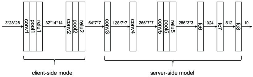
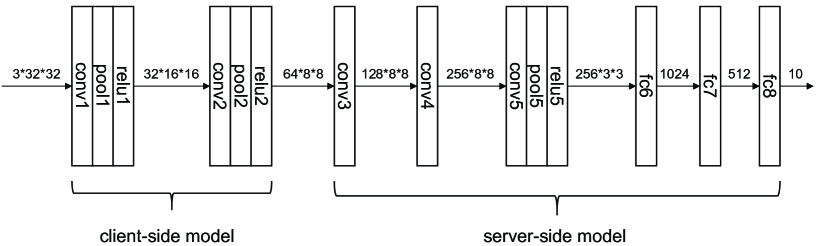
Implementation details. Unless otherwise stated, we set up clients and the server randomly selects of the total clients at each global iteration. We use AlexNet as the model, where we set up the first layers as the client-side model and the last layers as the server-side model. The detail of model architecture can be seen in Appendix E. The size of minibatch for the server-side model is and the number of local iterations is . The model is updated via SGD optimizer with learning rate .
Baselines. We first choose FL with logit adjustment as our baseline, that is, use (15) for local training of FL, which we refer to this method as FedLogit. Simultaneously, we select typical methods proposed to solve the issue of data heterogeneity as our baselines, such as FedLA (Zhang et al., 2022), FedDyn (Acar et al., 2021), FedProx (Li et al., 2020b), and FedDecorr (Shi et al., 2023).
Dataset. We adopt three popular image classification benchmark datasets, namely CIFAR10 (Krizhevsky et al., 2009), CIFAR100 (Krizhevsky et al., 2009) and CINIC10 (Darlow et al., 2018). CIFAR10 contains classes and CIFAR100 contains classes. Both of them have training samples and testing samples, and size of each image is . CINIC10 contains classes with training samples and testing samples, and size of each image is . To simulate the label skew distribution and generate local data for each client, we consider two label skew settings (Zhang et al., 2022): 1) quantity-based label skew and 2) distribution-based label skew. In quantity-based label skew, given clients and classes, we divide the data of each label into portions, and then randomly allocate portions of data to each client. Consequently, each client can obtain data from at most classes, indicating that there is the presence of class missing in the client data. We use to represent the degree of label skew, where a smaller implies stronger label skewness. In distribution-based label skew, for each selected client , we use Dirichlet distribution with classes to sample a probability vector and allocate a portion of of the samples in class to client . We use to denote the degree of skewness, where a smaller implies stronger label skewness.
5.2 Effect of Data Heterogeneity
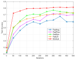
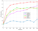
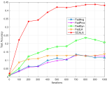
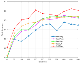
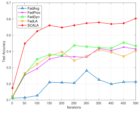
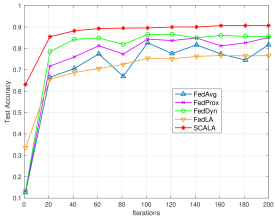
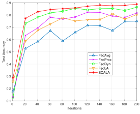
We first compare our method with previous works aimed at solving the issue of data heterogeneity. We select a quantity-based label skew with and , and a distribution-based label skew with and . For CIFAR10, CIFAR100, and CINIC10, we employ , , and global iterations. We run each experiment with random seeds and report the average accuracy and standard deviation as Table 1, where ‘-’ indicates the model fails to converge. Table 1 shows that our method significantly improves the model accuracy across various degrees of label skewness, particularly in settings where some classes of local data are missing, that is, under and configurations. The results demonstrate that our method mitigates the impact of highly skewed local label distribution. Additionally, we plot the test accuracy over global iteration in Figure 4, which further shows that our method SCALA not only enhances the model accuracy but also accelerates the convergence rate of the model.
5.3 Effect of Partial Client Participation
In this subsection, we study the robustness of SCALA to the proportion of clients participating at each global iteration. We select participation ratios of , , , and and set the degree of label skewness as and . The results are shown in Table 2. We observe that our method SCALA exhibits high robustness to the variation in client participation ratios, maintaining high accuracy across all settings. Note that, at higher client participation ratios, such as , all methods demonstrate higher accuracy because the increased client participation ensures that data from each class are sufficiently trained in each iteration, reducing the impact of global label distribution skew. As the client participation ratio decreases, SCALA significantly enhances the model performance. Thus our method SCALA is even applicable for spectrum constrained environments where only a few number of clients can participate in training at each global iteration.
| Method | CIFAR10 | CINIC10 | |||
|---|---|---|---|---|---|
| FedAvg | |||||
| FedProx | |||||
| FedLA | |||||
| Ours | |||||
| FedAvg | |||||
| FedProx | |||||
| FedLA | |||||
| Ours | |||||
| FedAvg | |||||
| FedProx | |||||
| FedLA | |||||
| Ours | |||||
| FedAvg | |||||
| FedProx | |||||
| FedLA | |||||
| Ours | |||||
5.4 Effect of Number of Clients
In this subsection, we ablate on the total number of clients. We set the total number of clients as , , , and and set the degree of label skewness as and . For experiments with clients and clients, we set of clients to participate in the training at each global iteration. For experiments with clients and clients, we set of clients to participate in the training at each global iteration. Results are shown in Table 3. We observe that SCALA exhibits better performance across various setting of the number of clients, particularly under more challenging settings with a higher number of clients. Specifically, even with clients, SCALA still achieves a to improvement in accuracy compared with FedAvg, which demonstrates that SCALA is more scalable in practice.
6 Conclusion
We proposed SCALA to address the issue of label distribution skew in SFL. We first concatenated activations output by participating clients to serve as the input of server-side model training. Then we proposed loss functions with logit adjustments for the server-side and client-side models. We performed detailed theoretical analysis and extensive experiments to verify the effectiveness of SCALA.
7 Impact Statements
This paper presents work whose goal is to advance the field of Machine Learning. There are many potential societal consequences of our work, none which we feel must be specifically highlighted here.
References
- Acar et al. (2021) Acar, D. A. E., Zhao, Y., Matas, R., Mattina, M., Whatmough, P., and Saligrama, V. Federated learning based on dynamic regularization. In International Conference on Learning Representations, 2021.
- Cao et al. (2019) Cao, K., Wei, C., Gaidon, A., Arechiga, N., and Ma, T. Learning imbalanced datasets with label-distribution-aware margin loss. Advances in neural information processing systems, 32, 2019.
- Chawla et al. (2002) Chawla, N. V., Bowyer, K. W., Hall, L. O., and Kegelmeyer, W. P. Smote: synthetic minority over-sampling technique. Journal of artificial intelligence research, 16:321–357, 2002.
- Chen et al. (2023) Chen, H., Wang, C., and Vikalo, H. The best of both worlds: Accurate global and personalized models through federated learning with data-free hyper-knowledge distillation. In The Eleventh International Conference on Learning Representations, 2023.
- Darlow et al. (2018) Darlow, L. N., Crowley, E. J., Antoniou, A., and Storkey, A. J. Cinic-10 is not imagenet or cifar-10. arXiv preprint arXiv:1810.03505, 2018.
- Fu et al. (2023) Fu, L., Zhang, H., Gao, G., Zhang, M., and Liu, X. Client selection in federated learning: Principles, challenges, and opportunities. IEEE Internet of Things Journal, pp. 1–1, 2023.
- Gawali et al. (2021) Gawali, M., Arvind, C., Suryavanshi, S., Madaan, H., Gaikwad, A., Bhanu Prakash, K., Kulkarni, V., and Pant, A. Comparison of privacy-preserving distributed deep learning methods in healthcare. In Medical Image Understanding and Analysis: 25th Annual Conference, MIUA 2021, Oxford, United Kingdom, July 12–14, 2021, Proceedings 25, pp. 457–471. Springer, 2021.
- Gupta & Raskar (2018) Gupta, O. and Raskar, R. Distributed learning of deep neural network over multiple agents. Journal of Network and Computer Applications, 116:1–8, 2018.
- Han et al. (2021) Han, D.-J., Bhatti, H. I., Lee, J., and Moon, J. Accelerating federated learning with split learning on locally generated losses. In ICML 2021 workshop on federated learning for user privacy and data confidentiality. ICML Board, 2021.
- Jamal et al. (2020) Jamal, M. A., Brown, M., Yang, M.-H., Wang, L., and Gong, B. Rethinking class-balanced methods for long-tailed visual recognition from a domain adaptation perspective. In Proceedings of the IEEE/CVF Conference on Computer Vision and Pattern Recognition, pp. 7610–7619, 2020.
- Jeon & Kim (2020) Jeon, J. and Kim, J. Privacy-sensitive parallel split learning. In 2020 International Conference on Information Networking (ICOIN), pp. 7–9, 2020.
- Kang et al. (2020) Kang, B., Xie, S., Rohrbach, M., Yan, Z., Gordo, A., Feng, J., and Kalantidis, Y. Decoupling representation and classifier for long-tailed recognition. In International Conference on Learning Representations, 2020.
- Krizhevsky et al. (2009) Krizhevsky, A., Hinton, G., et al. Learning multiple layers of features from tiny images. 2009.
- Lee et al. (2022) Lee, G., Jeong, M., Shin, Y., Bae, S., and Yun, S.-Y. Preservation of the global knowledge by not-true distillation in federated learning. In Oh, A. H., Agarwal, A., Belgrave, D., and Cho, K. (eds.), Advances in Neural Information Processing Systems, 2022.
- Li et al. (2020a) Li, T., Sahu, A. K., Talwalkar, A., and Smith, V. Federated learning: Challenges, methods, and future directions. IEEE Signal Processing Magazine, 37(3):50–60, 2020a.
- Li et al. (2020b) Li, T., Sahu, A. K., Zaheer, M., Sanjabi, M., Talwalkar, A., and Smith, V. Federated optimization in heterogeneous networks. Proceedings of Machine learning and systems, 2:429–450, 2020b.
- Luo et al. (2021) Luo, M., Chen, F., Hu, D., Zhang, Y., Liang, J., and Feng, J. No fear of heterogeneity: Classifier calibration for federated learning with non-iid data. In Ranzato, M., Beygelzimer, A., Dauphin, Y., Liang, P., and Vaughan, J. W. (eds.), Advances in Neural Information Processing Systems, volume 34, pp. 5972–5984. Curran Associates, Inc., 2021.
- McMahan et al. (2017) McMahan, B., Moore, E., Ramage, D., Hampson, S., and y Arcas, B. A. Communication-efficient learning of deep networks from decentralized data. In Artificial intelligence and statistics, pp. 1273–1282. PMLR, 2017.
- Menon et al. (2021) Menon, A. K., Jayasumana, S., Rawat, A. S., Jain, H., Veit, A., and Kumar, S. Long-tail learning via logit adjustment. In International Conference on Learning Representations, 2021.
- Michieli et al. (2022) Michieli, U., Toldo, M., and Ozay, M. Federated learning via attentive margin of semantic feature representations. IEEE Internet of Things Journal, 10(2):1517–1535, 2022.
- Mu et al. (2023) Mu, X., Shen, Y., Cheng, K., Geng, X., Fu, J., Zhang, T., and Zhang, Z. Fedproc: Prototypical contrastive federated learning on non-iid data. Future Generation Computer Systems, 143:93–104, 2023.
- Nguyen et al. (2020) Nguyen, H. T., Sehwag, V., Hosseinalipour, S., Brinton, C. G., Chiang, M., and Poor, H. V. Fast-convergent federated learning. IEEE Journal on Selected Areas in Communications, 39(1):201–218, 2020.
- Ren et al. (2020) Ren, J., He, Y., Wen, D., Yu, G., Huang, K., and Guo, D. Scheduling for cellular federated edge learning with importance and channel awareness. IEEE Transactions on Wireless Communications, 19(11):7690–7703, 2020.
- Rumelhart et al. (1986) Rumelhart, D. E., Hinton, G. E., and Williams, R. J. Learning representations by back-propagating errors. nature, 323(6088):533–536, 1986.
- Shang et al. (2022) Shang, X., Lu, Y., Huang, G., and Wang, H. Federated learning on heterogeneous and long-tailed data via classifier re-training with federated features. arXiv preprint arXiv:2204.13399, 2022.
- Shi et al. (2023) Shi, Y., Liang, J., Zhang, W., Tan, V., and Bai, S. Towards understanding and mitigating dimensional collapse in heterogeneous federated learning. In The Eleventh International Conference on Learning Representations, 2023.
- Tan et al. (2022) Tan, Y., Long, G., Liu, L., Zhou, T., Lu, Q., Jiang, J., and Zhang, C. Fedproto: Federated prototype learning across heterogeneous clients. In Proceedings of the AAAI Conference on Artificial Intelligence, volume 36, pp. 8432–8440, 2022.
- Thapa et al. (2022) Thapa, C., Arachchige, P. C. M., Camtepe, S., and Sun, L. Splitfed: When federated learning meets split learning. In Proceedings of the AAAI Conference on Artificial Intelligence, volume 36, pp. 8485–8493, 2022.
- Wang et al. (2020) Wang, J., Liu, Q., Liang, H., Joshi, G., and Poor, H. V. Tackling the objective inconsistency problem in heterogeneous federated optimization. Advances in neural information processing systems, 33:7611–7623, 2020.
- Wang et al. (2022) Wang, J., Qi, H., Rawat, A. S., Reddi, S., Waghmare, S., Yu, F. X., and Joshi, G. Fedlite: A scalable approach for federated learning on resource-constrained clients. arXiv preprint arXiv:2201.11865, 2022.
- Wang et al. (2021) Wang, L., Xu, S., Wang, X., and Zhu, Q. Addressing class imbalance in federated learning. In Proceedings of the AAAI Conference on Artificial Intelligence, volume 35, pp. 10165–10173, 2021.
- Woodworth et al. (2020) Woodworth, B. E., Patel, K. K., and Srebro, N. Minibatch vs local sgd for heterogeneous distributed learning. Advances in Neural Information Processing Systems, 33:6281–6292, 2020.
- Wu et al. (2023) Wu, D., Ullah, R., Rodgers, P., Kilpatrick, P., Spence, I., and Varghese, B. Communication efficient dnn partitioning-based federated learning. arXiv preprint arXiv:2304.05495, 2023.
- Xiao et al. (2022) Xiao, D., Yang, C., and Wu, W. Mixing activations and labels in distributed training for split learning. IEEE Transactions on Parallel and Distributed Systems, 33(11):3165–3177, 2022. doi: 10.1109/TPDS.2021.3139191.
- Xiao et al. (2017) Xiao, H., Rasul, K., and Vollgraf, R. Fashion-mnist: a novel image dataset for benchmarking machine learning algorithms. arXiv preprint arXiv:1708.07747, 2017.
- Yang et al. (2021a) Yang, H., Fang, M., and Liu, J. Achieving linear speedup with partial worker participation in non-IID federated learning. In International Conference on Learning Representations, 2021a.
- Yang et al. (2023) Yang, J., Liu, Y., and Kassab, R. Client selection for federated bayesian learning. IEEE Journal on Selected Areas in Communications, 41(4):915–928, 2023.
- Yang et al. (2021b) Yang, M., Wang, X., Zhu, H., Wang, H., and Qian, H. Federated learning with class imbalance reduction. In 2021 29th European Signal Processing Conference (EUSIPCO), pp. 2174–2178. IEEE, 2021b.
- Zhang et al. (2022) Zhang, J., Li, Z., Li, B., Xu, J., Wu, S., Ding, S., and Wu, C. Federated learning with label distribution skew via logits calibration. In International Conference on Machine Learning, pp. 26311–26329. PMLR, 2022.
- Zhang et al. (2023a) Zhang, J., Li, A., Tang, M., Sun, J., Chen, X., Zhang, F., Chen, C., Chen, Y., and Li, H. Fed-cbs: A heterogeneity-aware client sampling mechanism for federated learning via class-imbalance reduction. In International Conference on Machine Learning, pp. 41354–41381. PMLR, 2023a.
- Zhang et al. (2023b) Zhang, Y., Kang, B., Hooi, B., Yan, S., and Feng, J. Deep long-tailed learning: A survey. IEEE Transactions on Pattern Analysis and Machine Intelligence, 45(9):10795–10816, 2023b.
- Zhong et al. (2021) Zhong, Z., Cui, J., Liu, S., and Jia, J. Improving calibration for long-tailed recognition. In Proceedings of the IEEE/CVF Conference on Computer Vision and Pattern Recognition (CVPR), pp. 16489–16498, June 2021.
Appendix A Algorithm of SCALA
In this section, we summarizes the algorithm of SCALA in Algorithm 2. In each global iteration, the selected clients and the server collaborate to perform parallel SL over local iterations (line 8-21). In parallel SL phase, all selected clients synchronously execute local iterations (line 9-13 and line 18-20). The server-side model is centrally updated in each local iteration (line 14-15), where the loss functions for server-side and client-side models is adjust (line 15 and line 16). In FL phase, the client-side models are sent to the server for aggregation at the -th local iteration (line 21-24).
Appendix B Proof of Lemma 4.2
Given a dataset with classes, we can obtain the update of the classifier of label when using the softmax cross-entropy loss function as
| (19) |
where is the subset of dataset with label and . By introducing (B), we can obtain the update of the logit of label as
| (20) |
where is the averaged model feature of label defined as . Assume that model feature of label is similar, (B) can be rewritten as
| (21) |
When Assumption 4.1 holds, we can rewrite (B) as (4.2) and completes the proof.
Appendix C Proof of Lemma 4.3
Given a dataset with classes, we can obtain the update of the classifier of label when using the softmax cross-entropy loss function with logit adjustment as
| (22) |
By introducing (C), we can obtain the update of the logit of label as
| (23) |
Assume that model feature of label is similar, (C) can be rewritten as
| (24) |
When Assumption 4.1 holds, we can rewrite (C) as (4.3) and completes the proof.
Appendix D Proof of Theorem 4.4
We assume a mild condition where all labels are uniformly distributed except for label , that is, for all , . Then (4.3) can be rewritten as
| (25) |
Let denote , we have
| (26) |
and
| (27) |
According to (D) and (27), we have
| (28) |
Consequently, as approaches , will increase at a faster rate with the increase of . Given that when , we can draw the conclusion:
| (29) |
which completes the proof.
Appendix E The Details of Model Architecture of AlexNet
Appendix F More Experimental Results for Section 5.2
| Method | Fashion-MNIST | CIFAR10 | CIFAR100 | |||||
|---|---|---|---|---|---|---|---|---|
| FedAvg | ||||||||
| FedProx | ||||||||
| FedDyn | ||||||||
| FedDecorr | - | |||||||
| FedLogit | ||||||||
| FedLA | ||||||||
| Ours | ||||||||
| Method | CIFAR10 | CIFAR100 | ||||||
|---|---|---|---|---|---|---|---|---|
| SplitFedV1 | - | |||||||
| SplitFedV2 | - | - | - | - | ||||
| SplitFedV3 | ||||||||
| SFLLocalLoss | ||||||||
| Ours | ||||||||
| Method | Fashion-MNIST | CINIC10 | ||||||
|---|---|---|---|---|---|---|---|---|
| SplitFedV1 | ||||||||
| SplitFedV2 | - | |||||||
| SplitFedV3 | ||||||||
| SFLLocalLoss | ||||||||
| Ours | ||||||||
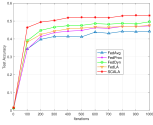
We conduct more experiments to compare our proposed method with compared FL algorithms on Fashion-MNIST, CIFAR10, and CIFAR100. Fashion-MNIST (Xiao et al., 2017) contains classes, with training samples and testing samples. Each image size of Fashion-MNIST is . We run each experiment with random seeds and report the average accuracy and standard deviation as Table 4. Additionally, we plot the test accuracy of the global model at each global iteration in Figure 7. These results further demonstrate our proposed SCALA improves model performance in the setting with label distribution skew.
In addition, we compare the proposed method with some of the latest SFL algorithms, such as SplitFedV1 (Thapa et al., 2022), SplitFedV2 (Thapa et al., 2022), SplitFedV3 (Gawali et al., 2021), and SFLLocalLoss (Han et al., 2021), as shown in Table 5 and Table 6. Specifically, in SplitFedV1, the server-side models and local-side models of participating clients are executed separately in parallel and then aggregated to obtain the global model at each global iteration. SplitFedV2 processes the forward-backward propagations of the server-side model sequentially with respect to the activations of clients (no FedAvg of the server-side models). In SplitFedV3, the client-side models are unique for each client and the server-side model is an averaged version. And SFLLocalLoss introduces an auxiliary network (local classification) at the client side, where clients update local models based on the local loss functions. Table 5 and Table 6 indicate that our method markedly boosts the performance of SFL and facilitating its widespread adoption for SFL in label distribution skew.
Appendix G Effect of Number of Local Iterations
| Method | ||||||||
|---|---|---|---|---|---|---|---|---|
| FedAvg | ||||||||
| FedProx | ||||||||
| FedLA | ||||||||
| Ours | ||||||||
We ablate on the number of local iterations on CIFAR10. We set the number of local iterations as , , , and and set the degree of label skewness as and . The number of the global iterations is uniformly set to . As shown in Table 7, the accuracy of each method initially increases with more local iterations but subsequently decreases. This is because the model is not sufficiently trained when the number of local iterations is small, leading to an enhancement in accuracy as local iterations increase. However, when the number of local iterations is substantial, the local models tend to bias towards local optima, adversely affecting the model performance. Nevertheless, our method consistently outperforms other methods.
Appendix H Effect of Splitting Points Selection
| Dataset | Splitting point selection | ||||
|---|---|---|---|---|---|
| CINIC10 | S1 | ||||
| S2 | |||||
| S3 | |||||
| S4 | |||||
| S5 | |||||
| CIFAR10 | S1 | ||||
| S2 | |||||
| S3 | |||||
| S4 | |||||
| S5 | |||||
| CIFAR100 | S1 | ||||
| S2 | |||||
| S3 | |||||
| S4 | |||||
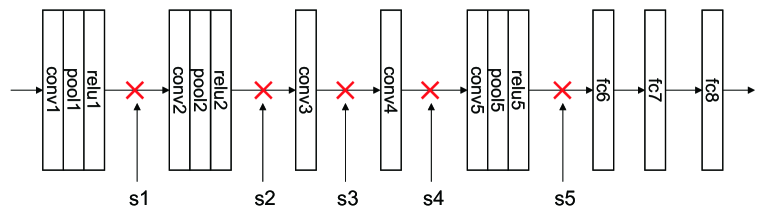
| S5 |
We ablate on the different splitting points, with the splitting points shown in the figure 8 as s1, s2, s3, s4, and s5. We select a quantity-based label skew with and , and a distribution-based label skew with and . For CIFAR10, CIFAR100, and CINIC10, we employ , , and global iterations, respectively. We run each experiment with random seeds and report the average accuracy as shown in Table 8. As indicated in Table 8, the model accuracy decreases as the depth of the split increases. This experimental result demonstrates that deploying more models on the server to utilize concatenated activations for centralized training can effectively mitigate the model drift in label distribution skew, thereby improving the model performance.