Fate of Two-Particle Bound States in the Continuum in non-Hermitian Systems

Abstract

We unveil the existence of two-particle bound state in the continuum (BIC) in a one-dimensional interacting nonreciprocal lattice with a generalized boundary condition. By applying the Bethe-ansatz method, we can exactly solve the wavefunction and eigenvalue of the bound state in the continuum band, which enable us to precisely determine the phase diagrams of BIC. Our results demonstrate that the non-reciprocal hopping can delocalize the bound state and thus shrink the region of BIC. By analyzing the wavefunction, we identify the existence of two types of BICs with different spatial distributions and analytically derive the corresponding threshold values for the breakdown of BICs. The BIC with similar properties is also found to exist in another system with an impurity potential.

Introduction- An intriguing property of Non-Hermitian systems is the sensitivity of wavefunctions and spectra to boundary conditions and local impurity. Intensive studies have unveiled that non-Hermitian nonreciprocal systems can exhibit some novel non-Hermitian phenomena, e.g., non-Hermitian skin effect (NHSE) LeeCH ; 13 ; 15 ; 16 ; 17 ; 18 and scale-free localization LiLH2021 ; Murakami ; GuoCX2023 ; WangZ2023 ; Bergholtz2023 , characterized by the emergence of diverse localizing behaviors and changes of spectrum structures when translational invariance is locally broken, either by introducing an impurity or by tuning the boundary coupling strength LiuYX2021 ; CXGuo2021 . While most novel phenomena and concepts about the non-Hermitian effects are built based on the non-interacting systems, recently there is growing interest in exploring non-Hermitian phenomena in interacting systems XuZ ; ZhangDW ; Nori2020 ; Fukui ; ZhengMC ; LiLH2024 .

The concept of bound state in the continuum (BIC) was initially proposed by von Neumann and Wigner, which refers to the eigenenergies of the bound states that can be embedded in the continuum Neumann29 ; Hsu16 . Recently, BICs attracted much renewed interest both theoretically and experimentally Zhang23 ; Zhen14 ; Kang23 ; Qian24 ; Vaidya21 ; Cerjan20 ; Yuan20 ; Xiao17 . The BICs are found to be present in many physical systems, including the Hubbard modelZhangJM12 ; ZhangJM13 ; Valle14 ; YAshida22 ; Sugimoto23 ; WZhang23 ; Huang23 , optical systems Koshelev18 ; Cao20 ; Kravtsov20 ; Fan19 ; Han19 , etc, and have caused many applications such as enhanced optical nonlinearity Carletti18 ; Bulgakov14 ; Krasikov18 , sensing Yanik11 ; Liu17 ; Romano19 , lasers Kodigala17 ; Song18 ; Midya18 ; Yu21 , and filtering Foley14 . Usually, the emergence of BIC in a single particle system requires certain exotic potentials. For multi-particle systems, BIC can be created via the interplay of local potential and particle-particle interaction ZhangJM12 ; ZhangJM13 ; Sugimoto23 ; WZhang23 . It has been demonstrated that BICs can be engineered in impurity systems by adding inter-particle interaction ZhangJM12 ; ZhangJM13 . Meanwhile, edge states in the continuum are also found in interacting topological models Liberto16 ; Gorlach17 . Usually, bound states must have quantized energies in a Hermitian system, whereas free states form a continuum. However, this principle may fail for non-Hermitian systems MaGC . Some recent works demonstrate that continuum of bound states can occur in non-Hermitian systems MaGC ; ChongYD ; ChenG . In the presence of NHSE, a local bound state may be delocalized depending on the competition between non-reciprocal hopping and impurity strength. Studies on the impurity model in non-reciprocal lattices reveals that the bound state disappears when it touches the continuum of spectrum LiuYX2020 . As most previous studies of BIC focused on the Hermitian systems, this raises our interest to pursue the BIC in non-Hermitian system with non-reciprocal hopping and interaction.

In this Letter, we study two-particle BICs in non-Hermitian lattices and unveil their specific feature and fate under the influence of the nonreciprocal hopping. To be concrete, we consider two interacting bosons in a nonreciprocal lattice with GBC or an impurity potential. Although the model is generally not solvable, we demonstrate that the BIC can be exactly solved with Bethe-ansatz wavefunction. The analytical expression of wavefunction and bound energy enables us to determine the phase diagram of BIC exactly. We unveil the existence of two kinds of BICs, characterized by different spatial distributions, which are delocalized by increasing the nonreciprocal hopping. By analyzing the wavefunction, we derive analytical expressions of threshold values for the breakdown of BICs. Our analytical results provide a firm ground for understanding the fate of BICs in non-Hermitian systems.

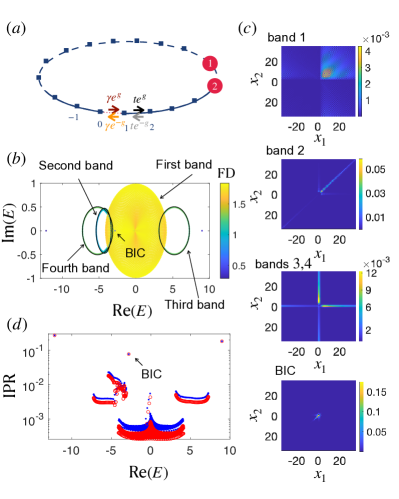
Figure 1: (a) Schematics of the two-particle Hatano-Nelson model with GBCs described in Eq. (Fate of Two-Particle Bound States in the Continuum in non-Hermitian Systems). The dark blue squares represent the lattice. The red circles represent two particles. (b) The real and imaginary parts of spectra of the system with parameters $(g,\gamma,U)=(0.25,5,-3.5)$. The color of each dot represents the fractal dimension $\Gamma$ of different eigenstates. The three black circles from left to right are the fourth band $E_{4}=-(\gamma+1/\gamma)+2\cos(k-ig)$, the second band $E_{2}=-\sqrt{U^{2}+16\cos^{2}(K-ig)}$, and the third band $E_{3}=\gamma+1/\gamma+2\cos(k-ig)$, respectively. The length of the lattice is $N=2M=90$. (c) From top to bottom, we display the density distribution of the wave function in the first, second, third (or fourth) bands and BIC, respectively. (d). IPRs for eigenstates with the corresponding real parts of eigenvalues $Re(E)$ for the system with parameters $(g,\gamma,U)=(0.25,5,-3.5)$. The length of the lattice is chosen to be $N=70$ (blue dots) and $N=90$ (red circles).

Model and spectrum.- The model we consider consists of two identical spinless bosons in the Hatano-Nelson model with generalized boundary conditions (GBCs), as illustrated in Fig 1 (a), which can be described by

$$\hat{H} =\sum_{x=-L,x\neq 0}^{M}\left[-t\left(e^{g}\hat{a}_{x}^{{\dagger}}\hat{a}_{x+1}+e^{-g}\hat{a}_{x+1}^{{\dagger}}\hat{a}_{x}\right)+\frac{U}{2}\hat{a}_{x}^{{\dagger}}\hat{a}_{x}^{{\dagger}}\hat{a}_{x}\hat{a}_{x}\right]$$

$$-\gamma\left(e^{g}\hat{a}_{0}^{{\dagger}}\hat{a}_{1}+e^{-g}\hat{a}_{1}^{{\dagger}}\hat{a}_{0}\right),$$ (1)

where $\hat{a}_{x}^{{\dagger}}$ $(\hat{a}_{x})$ is the boson creation (annihilation) operator at site $x$, $te^{g}$ and $te^{-g}$ are imbalanced hopping amplitudes, $\gamma$ represents the boundary strength, and $t,~{}\gamma,~{}g\in\mathbb{R}$. $U$ is the interaction strength between particles and we shall consider the case of attractive interaction with $U<0$. We set $t=1$ as the unit of energy in the following calculation. For clear numerical presentation, we put the boundary in the middle of the lattice, and we label the lattice sites from $-L$ to $M$ and set $\hat{a}_{-L}^{{\dagger}}=\hat{a}_{M+1}^{{\dagger}}$, $\hat{a}_{-L}=\hat{a}_{M+1}$. $L=M-1$ for even lattice, $L=M$ for odd lattice.

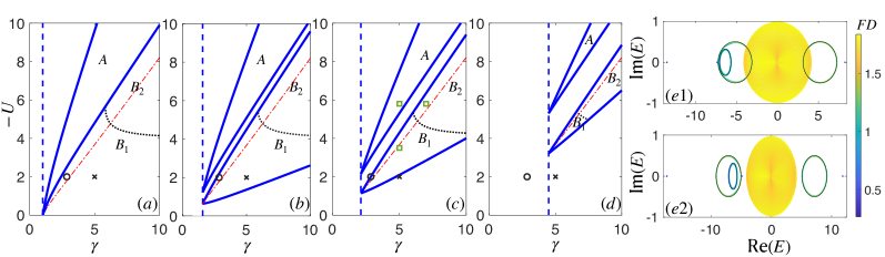
Figure 2: (a)-(d) The phase diagram for the bound state (16) with parameter $g=0$, $0.15$, $0.25$, and $0.5$, respectively. The bound state with $E_{b1}$ exists in the region $A$, which is below all four real parts of continuum bands. In the region of $B_{1}$, the state with energy $E_{b2}$ is a bound state in the first continuum band $2\cos(k_{1}+ig)+2\cos(k_{2}+ig)$. In the region of $B_{2}$, this state is below the real part of the first and third continuum bands and above the real part of the second and fourth continuum bands. The condition that distinguishes those two regions is $E_{b1}=4\cosh g$, which is represented by the black dotted lines. The blue dashed lines represent $\gamma=e^{3|g|}$. When $\gamma<e^{3|g|}$, none of the third and fourth bands and bound state (16) exist. The red dotted-dashed lines represent $g_{1}=g_{2}$, where $g_{1}=\ln h(1/\gamma-\gamma-U)$ and $g_{2}=\ln\left[\gamma/h(1/\gamma-\gamma-U)\right]/2$ with $h(x)=(\sqrt{x^{2}+4}+|x|)/2$. The black crosse represents $(\gamma,U)=(2.855434,-2)$ and the black circle represents $(\gamma,U)=(5,-2)$. The three green squares in (c) represent $(\gamma,U)=(5,-3.5)$, $(5,-5.8)$, and $(7,-5.8)$, which are points in the regions $B_{1}$, $A$, and $B_{2}$, respectively. (e) The spectra of the system with parameters $(g,\gamma,U)=(0.25,5,-5.8)$ and $(g,\gamma,U)=(0.25,5,-5.8)$.

With wave function $|\psi\rangle=\sum_{x_{1}\leqslant x_{2}}\left[\sqrt{2}-(\sqrt{2}-1)\delta_{x_{1},x_{2}}\right]u(x_{1},x_{2})\hat{a}_{x_{1}}^{{\dagger}}\hat{a}_{x_{1}}^{{\dagger}}|0\rangle$, the eigenvalue equation $H|\psi\rangle=E|\psi\rangle$ can be rewritten as homogeneous linear difference equation about $u(x_{1},x_{2})$:

$$-\sum_{a=\pm 1}te^{ag}\left[u(x_{1}+a,x_{2})+u(x_{1},x_{2}+a)\right]$$ (2)

$$+U\delta_{x_{1},x_{2}}u(x_{1},x_{2})=E u(x_{1},x_{2}),$$

and the equations of GBCs are

$$-\sum_{a=\pm 1}te^{ag}u(0,x_{2}+a)+U\delta_{0,x_{2}}u(0,x_{2})$$ (3)

$$-\gamma e^{g}u(1,x_{2})-e^{g}u(-1,x_{2})=E u(0,x_{2}),$$

and

$$-\sum_{a=\pm 1}te^{ag}u(1,x_{2}+a)+U\delta_{1,x_{2}}u(1,x_{2})$$ (4)

$$-e^{g}u(2,x_{2})-\gamma e^{g}u(0,x_{2})=E u(1,x_{2}).$$

In the absence of interaction ($U=0$), the model reduces to the Hatano-Nelson (HN) model Hatano96 ; Hatano97 with GBC LiLH2021 ; CXGuo2021 , which can be exactly solvable in the whole parameter region CXGuo2021 . The boundary parameter $\gamma$ interpolates the OBC($\gamma=0$) to PBC ($\gamma=1$).

Our goal is to address the eigenvalue problem, with a focus on the bound states where both particles are confined near the boundary sites at $x=0$ and $1$. To get a straightforward view of the BIC, we display the spectra of the system with $\gamma=5$ in Fig. 1(b), including four complex continuum bands SM , a BIC and two separated bound states above or below the bands, where eigenvalues of the three bound states are all real. The spectral of the first band is given by $2\cos(k_{1}-ig)+2\cos(k_{2}-ig)$ with $k_{1},~{}k_{2}\in\left[0,2\pi\right)$ and interval of real parts in $\left[-4\cosh g,~{}4\cosh g\right]$, corresponding to scattering states of two particles in the HN lattice. In comparison with free particles, the scattering eigenstates have phase shifts at boundaries and the location where the two particles interact. A typical distribution of random chosen wavefunction in this band is displayed in the first row of Fig. 1(c). The spectral of the second band is given by $-\sqrt{U^{2}+16\cos^{2}(K-ig)}$ for $U<0$ and $\sqrt{U^{2}+16\cos^{2}(K-ig)}$ for $U>0$ with $K\in\left[0,2\pi\right)$, which corresponds to the delocalized molecule states. The interval of the real part is $\left[-\sqrt{U^{2}+16\cosh^{2}g},~{}-\sqrt{U^{2}-16\sinh^{2}g}\right]$ for $U<-4\sinh|g|$ and $\left[\sqrt{U^{2}-16\sinh^{2}g},~{}\sqrt{U^{2}+16\cosh^{2}g}\right]$ for $U>4\sinh|g|$. The density distribution of a typical state in this band is presented in the second row of Fig. 1(c). It is shown that two particles are bound together and distribute along the diagonal line. Here the asymmetric distribution along the diagonal line is attributed to the nonreciprocal hopping. States in the third and fourth bands correspond to scattering states with one particle bound around the boundary, with the corresponding density distribution shown in the third row of Fig. 1(c). The energy of the bound particle can be either of $\pm(\gamma+1/\gamma)$, while the other is $2\cos(k-ig)$ with $k\in\left[0,2\pi\right)$. Thus the real part of these two bands covers $\left[\gamma+1/\gamma-2\cosh g,~{}\gamma+1/\gamma+2\cosh g\right]$ and $\left[-\gamma-1/\gamma-2\cosh g,~{}-\gamma-1/\gamma+2\cosh g\right]$, respectively.

To characterize the distribution properties of states in these four bands and bound states, we can numerically calculate their fractal dimension (FD) defined as

$$\text{FD}_{j}=-\lim_{N\rightarrow\infty}\ln(\text{IPR}_{j})/\ln(N),$$ (5)

where $\text{IPR}_{j}=\sum_{x_{1},x_{2}}|u_{j}(x_{1},x_{2})|^{4}$ is the inverse participation ratio. The FD tends to $2$, $1$, and $0$ for the states in the first band, in the other bands, and bound states, respectively, as displayed in Fig. 1 (b). To see it more clearly, we also display the corresponding IPRs with different lattice sizes in Fig. 1(d). It is shown that the IPRs of states in continuum bands change with the lattice size, whereas IPRs of the three bound states are not sensitive to the change of lattice size. A BIC corresponds to the bound state with energy falling in $\left[-4\cosh g,~{}4\cosh g\right]$.

Analytical solution of BIC.- Although general eigenstates of our model (1) are not solvable, we show that the BIC can be analytically derived by taking the Bethe ansatz type (BAT) wavefunction:

$$u(x_{1},x_{2}) =\sum_{n=1}^{3}\sum_{Q,P}\sum_{\epsilon_{P}=\pm 1}\theta(x_{Q_{1}}<x_{Q_{2}})$$ (6)

$$\times A_{n}(\epsilon_{P}P)e^{i\sum_{j}(\epsilon_{P_{1}}k_{P_{j}}+ig)x_{Q_{j}}},$$

where $Q=(Q_{1},Q_{2})$ and $P=(P_{1},P_{2})$ are two arrangements of $(1,2)$. The index $n$, together with $\theta(x_{Q_{1}}<x_{Q_{2}})$ can distinguish the six regions (see supplementary materia for details SM ). Note that the wavefunction in $x_{1}>x_{2}$ can be determined by the wavefunction in $x_{1}<x_{2}$, due to the exchange symmetry $u(x_{1},x_{2})=u(x_{2},x_{1})$, so $A_{n}(\epsilon_{P}P)$ is independent of the ordering of $x_{1}$ and $x_{2}$. Eq. (6) is just a formal solution. To be an eigenstate, the BAT wavefunction should satisfy the boundary equations. Inserting Eq. (6) into Eqs. (3) and (4) gives us a set of homogeneous linear equations about $A_{n}(\epsilon_{P_{1}}P_{1},\epsilon_{P_{2}}P_{2})$, which can determine these values as well as $k_{1}$ and $k_{2}$. The wavefunction can be exactly expressed as

$$u_{b}(x_{1},x_{2})=u_{b,0}(x_{1},x_{2})e^{-g(x_{1}+x_{2})},$$ (7)

where

$$u_{b,0}(x_{1},x_{2})=\left\{\begin{array}[]{cc}f_{1}(x_{1},x_{2}),{}{}{}{}{}{}&0<x_{1}\leqslant x_{2}\\ f_{2}(x_{1},x_{2}),{}{}{}{}{}{}&x_{1}\leqslant 0<x_{2},\\ -f_{1}(-x_{2},-x_{1}),&x_{1}\leqslant x_{2}\leqslant 0\\ f_{1}(x_{2},x_{1}),{}{}{}{}{}{}&0<x_{2}<x_{1},\\ f_{2}(x_{2},x_{1}),{}{}{}{}{}{}&x_{2}\leqslant 0<x_{1},\\ -f_{1}(-x_{1},-x_{2}),&x_{2}<x_{1}\leqslant 0,\\ \end{array}\right.$$ (14)

with

$$f_{1} (x_{1},x_{2})=\frac{e^{ik_{1}}-\gamma^{2}e^{-ik_{1}}}{2i\gamma\sin k_{1}}e^{ik_{1}x_{1}+ik_{2}x_{2}}$$ (15)

$$+\frac{e^{ik_{1}}(\gamma^{2}-1)}{2i\gamma\sin k_{1}}e^{-ik_{1}x_{1}+ik_{2}x_{2}}-\frac{e^{ik_{1}}(1-\gamma^{2})}{2i\gamma\sin k_{2}}e^{ik_{2}x_{1}-ik_{1}x_{2}},$$

and

$$f_{2}(x_{1},x_{2})=e^{ik_{1}x_{1}+ik_{2}x_{2}}-e^{ik_{1}+ik_{2}}e^{-ik_{2}x_{1}-ik_{1}x_{2}}.$$ (16)

To correctly describe a bound state, from (7), we see that $|e^{ik_{1}}|>e^{|g|}$ and $|e^{ik_{2}}|<e^{-|g|}$ are required. Meanwhile, $k_{1,2}$ are given by

$$\gamma=e^{-ik_{2}},~{}~{}~{}1/\gamma-\gamma-U=e^{ik_{1}}-e^{-ik_{1}}.$$ (17)

The exact energy of bound state $E_{b}=-2\cos k_{1}-2\cos k_{2}$ has two possibilities: $E_{b1}=-1/\gamma-\gamma-\sqrt{(\gamma-1/\gamma+U)^{2}+4}$ for $1/\gamma-\gamma>U$ and $E_{b2}=-1/\gamma-\gamma+\sqrt{(\gamma-1/\gamma+U)^{2}+4}$ for $1/\gamma-\gamma<U$. Here, we can see that the energy of the bound state is independent of the parameter $g$. However, the wavefunction is different from the Hermitian case by a factor of $e^{-g(x_{1}+x_{2})}$.

Phase diagram of BIC.- To maintain the state of $E_{b}=E_{b1}$ as a bound state, the condition $U_{1,1}<U<U_{1,2}$ must be satisfied, where $U_{1,1}=2(e^{|g|}/\gamma-e^{-|g|}\gamma)\cosh g$ and $U_{1,2}=1/\gamma-\gamma-2\sinh|g|$, which forms areas $A$. This region shrinks with increasing $g$, as shown in Fig. 2 (a)-(d). Since $E_{b1}<\min\{-4\cosh g,~{}-\sqrt{U^{2}+16\cosh^{2}g},~{}\pm(\gamma+1/\gamma)-2-2\cosh g\}$, the bound state is below all four continuum bands in the real axis and thus is not a BIC. A typical spectrum structure for the system marked by the square in the region of $A$ is displayed in Fig. 2 (e1). The two transfer points $U_{1,1}$ and $U_{1,2}$ are determined by the touching points that $E_{b1}$ touches the second and fourth continuum bands, respectively.

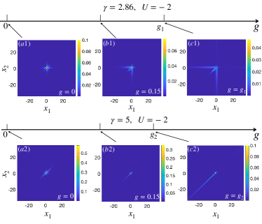
Figure 3: (a1)-(c1) The density distribution of the BIC with $g=0$, $g=0.15$, and $g=g_{1}$ for the system with $\gamma=2.86$ and $U=-2$. (a2)-(c2) The density distribution of the BIC with $g=0$, $g=0.15$, and $g=g_{2}$ for the system with $\gamma=5$ and $U=-2$.

Similarly, the condition to maintain the state of $E_{b}=E_{b2}$ as a bound state is $U_{2,1}<U<U_{2,2}$ with $U_{2,1}=1/\gamma-\gamma+2\sinh|g|$ and $U_{2,2}=-2(e^{|g|}/\gamma+e^{-|g|}\gamma)\sinh|g|$, which forms areas $B_{1,2}$ as shown in Fig. 2. As the value of $g$ increases, the corresponding regions also shrink. The points $U=U_{2,1}$ and $U=U_{2,2}$ are just the touching points of $E_{b2}$ with second and fourth bands. We can prove that $E_{b2}>\max\{-\sqrt{U^{2}+16\cos^{2}(\pi/2-ig)}~{},-(\gamma+1/\gamma)+2\cosh(g)\}$ and $E_{b2}<(\gamma+1/\gamma)-2\cosh(g)$. Thus this bound state can not fall in the second to fourth bands. It may fall within the first continuum band, if an additional condition $E_{b2}>-4\cosh g$ is fulfilled, which gives rise to the area $B_{1}$ as displayed in Fig. 2. In the parameter region $B_{1}$ there exists a BIC with a typical spectrum structure depicted in Fig. 1(b). As a comparison, a typical spectrum for the system marked by the square in region of $B_{2}$ is displayed in Fig. 2 (e2).

Although the parameter $g$ does not change the energy of the bound state, it changes the continuous spectrum and affects the fate of BIC by modifying the wavefunction. With the increase in $g$, the first band expands in both directions along the real axis, while the second and fourth bands also increase in size. When the $2nd$ or $4th$ band touches the bound energy, the bound state merges into this band and vanishes. The touching point gives rise to a threshold value $g_{1}=\ln h(1/\gamma-\gamma-U)$ with $h(x)=(\sqrt{x^{2}+4}+|x|)/2$ or $g_{2}=\ln\left[\gamma/h(1/\gamma-\gamma-U)\right]/2$, determined by either $E_{b2}=-\gamma-1/\gamma+2\cosh|g_{1}|$ or $E_{b2}=-\sqrt{U^{2}-16\sinh^{2}g}_{2}$. In the parameter space spanned by $\gamma$ and U, the relation $g_{1}(\gamma,U)=g_{2}(\gamma,U)$ gives a dividing line distinguishing which band expanding to $E_{b2}$ first, as shown in Fig. 2 (a)-(d) by the dashed-dotted red lines. The bound state above the dividing line merges into the fourth band and vanishes when $g>g_{1}$, whereas the bound state below the dividing line merges into the second band when $g>g_{2}$. Besides the threshold values determined by different relations, the BICs above and below the dividing line exhibit different spatial distributions, as displayed in Fig. 3 (a1)-(c1) and Fig. 3 (a2)-(c2), respectively. Here, density distributions shown in Fig. 3 (a1)-(c1) correspond to the circles in Fig. 2 (a)-(c), and the ones in Fig. 3 (a2) and (b2) correspond to the crosses in Fig. 2 (a) and (b), respectively.

With the increase in $g$, it can be found from Fig. 3 that the BIC is delocalized either along the $x_{1}$ and $x_{2}$ axis or the diagonal direction $x_{1}=x_{2}$. The wavefunction along the axis-$x_{1}$ is $u_{b}(x_{1},0)=e^{-gx_{1}}u_{b,0}(x_{1},0)$ with

$$u_{b,0}(x_{1},0)=\left\{\begin{array}[]{cc}e^{ik_{2}x_{1}}-e^{ik_{1}+ik_{2}}e^{-ik_{1}x_{1}},&x_{1}>0,\\ e^{ik_{1}x_{1}}-e^{ik_{1}+ik_{2}}e^{-ik_{2}x_{1}},&x_{1}\leqslant 0.\\ \end{array}\right.$$ (20)

Eq. (20) is the superposition of two exponentially decaying wave functions $e^{-ik_{1}x_{1}}$ and $e^{ik_{2}x_{1}}$ with exponential decay factors (EDFs) $L_{h1}=-\text{Im}(k_{1})$ and $L_{h2}=\text{Im}(k_{2})$, respectively. From Eq. (17), it follows that $L_{h1}=\ln h(1/\gamma-\gamma-U)$ with $h(x)=(\sqrt{x^{2}+4}+|x|)/2$ ik1 and $L_{h2}=\ln\gamma$. Since $L_{h1}<L_{h2}$ is always fulfilled for BIC, we see that $u_{b}(x_{1},0)$ is completely delocalized when $g=L_{h1}\equiv g_{1}$. The wavefunction $u_{b}(0,x_{2})$ has the same properties due to the exchange symmetry of $x_{1}$ and $x_{2}$. The wavefunction (14) along the diagonal line $x_{1}=x_{2}$, i.e., $u_{b,0}(x_{1},x_{1})$, also has two EDFs: $L_{d1}=\text{Im}(k_{1}+k_{2})=\ln\left[\gamma/h(1/\gamma-\gamma-U)\right]$ and $L_{d2}=\text{Im}(k_{2}-k_{1})=\ln\left[\gamma h(1/\gamma-\gamma-U)\right]$. Since $L_{d1}<L_{d2}$, $u_{b}(x_{1},x_{2})$ is completely delocalized along the diagonal line when $g=L_{d1}/2\equiv g_{2}$. From the analysis of wavefuntion of BIC, we see clearly that the threshold value for the breakdown of BIC is given by $g=\min\{g1,g2\}$.

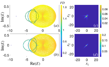
Figure 4: (a) (b) The real and imaginary parts of spectra of the system with parameters $(g,V,U)=(0.15,-2.6,-2)$ and $(g,V,U)=(0.15,-3.5,-2)$, respectively. The color of each dot represents the fractal dimension $\Gamma$ of different eigenstates. The two black circles from left to right are the third band $E_{3}=-\sqrt{V^{2}+4}+2\cos(k-ig)$ and the second band $E_{2}=-\sqrt{U^{2}+16\cos^{2}(K-ig)}$, respectively. (c) (d) The density distribution of the BIC for the system with parameters $(g,V,U)=(0.15,-2.5,-2)$ and $(g,V,U)=(0.15,-3.5,-2)$, respectively. The length of the lattice is $2M+1=91$.

BIC in the impurity model.- Next we show that BIC can be also identified in the two-particle Hatano-Nelson model with an impurity under periodic boundary condition, described by

$$\hat{H}= \sum_{x=-L}^{M}\left[-e^{g}\hat{a}_{x}^{{\dagger}}\hat{a}_{x+1}-e^{-g}\hat{a}_{x+1}^{{\dagger}}\hat{a}_{x}+\frac{U}{2}\hat{a}_{x}^{{\dagger}}\hat{a}_{x}^{{\dagger}}\hat{a}_{x}\hat{a}_{x}\right]$$

$$+V\hat{a}_{0}^{{\dagger}}\hat{a}_{0},$$ (21)

where the impurity strength $V<0$ and $U<0$. Similarly, BIC can be solved exactly by applying the BA method. The corresponding energy $E_{BIC}=-\sqrt{V^{2}+4}+\sqrt{(V-U)^{2}+4}$ and the conditions for existence of BIC are $V+2\sinh|g|<U<V-e^{-2|g|}V-2\sinh^{2}(2|g|)\frac{V+\sqrt{V^{2}+4}}{2}$ and $E_{BIC}>-4\cosh g$. For this system, there are three continuum bands, the first band $2\cos(k_{1}-ig)+2\cos(k_{2}-ig)$ with $k_{1},~{}k_{2}\in\left[0,2\pi\right)$, the second band $\text{sign}(U)\sqrt{U^{2}+16\cos^{2}(K-ig)}$ with $K\in\left[0,2\pi\right)$, and the third band $-\sqrt{V^{2}+4}+2\cos(k-ig)$, with $k\in\left[0,2\pi\right)$, as shown in Fig. 4 (a) and (b).

The BICs also exhibit two kinds of different distributions, as displayed in Fig. 4 (c) and (d), leading to different ways to compete with the non-reciprocal term. The first way is that the increase of $g$ causes the BIC to lose localization along the axis of $x_{1}$ and $x_{2}$ when $g_{1}(V,U)<g_{2}(V,U)$, where $g_{1}(V,U)=\ln h(V-U)$ and $2g_{2}(V,U)=\ln[h(V)/h(V-U)]$ are the minimum EDFs of the wavefunction of BIC along the $x_{1}$ and $x_{2}$ axis and the diagonal direction $x_{1}=x_{2}$ with $g=0$. This BIC will merge into the third band. The second way is that as the value of $g$ increases, the wavefunction of BIC becomes extended along the diagonal direction when $g_{2}(V,U)<g_{1}(V,U)$. This BIC will merge into the second band.

Summary.- Using Bethe ansatz method, we have obtained the exact solution for the BIC in the two-particle interacting Hatano-Nelson model with either generalized boundary conditions or an impurity potential. Our results demonstrate that the interplay of interactions, boundary potential and non-reciprocal hopping can give rise to two types of BICs with different spatial distributions. The exact wave function and energy of BIC enable us to get a precise phase diagram of BICs with the boundaries marking the emergence and breakdown of BICs being analytically determined.

- (1) S. Yao and Z. Wang, Edge States and Topological Invariants of Non-Hermitian Systems, Phys. Rev. Lett. 121, 086803 (2018).
- (2) F. K. Kunst, E. Edvardsson, J. C. Budich, and E. J. Bergholtz, Biorthogonal bulk-boundary correspondence in non-Hermitian systems, Phys. Rev. Lett. 121, 026808 (2018).
- (3) C. H. Lee and R. Thomale, Anatomy of skin modes and topology in non-hermitian systems, Phys. Rev. B 99, 201103(R) (2019).
- (4) K. Yokomizo and S. Murakami, Non-Bloch Band Theory of Non-Hermitian Systems, Phys. Rev. Lett. 123, 066404 (2019).
- (5) K. Zhang, Z. Yang, and C. Fang, Correspondence between winding numbers and skin modes in non-hermitian systems, Phys. Rev. Lett. 125, 126402 (2020).
- (6) N. Okuma, K. Kawabata, K. Shiozaki and M. Sato, Topological Origin of Non-Hermitian Skin Effects, Phys. Rev. Lett. 124, 086801 (2020).
- (7) L. Li, C. H. Lee, and J. Gong, Impurity induced scale-free localization, Commun. Phys. 4, 42 (2021).
- (8) K. Yokomizo and S. Murakami, Scaling rule for the critical non-Hermitian skin effect, Phys. Rev. B 104, 165117 (2021).
- (9) C.-X. Guo, X. Wang, H. Hu, and S. Chen, Accumulation of scale-free localized states induced by local non-Hermiticity, Phys. Rev. B 107, 134121 (2023).
- (10) B. Li, H.-R. Wang, F. Song, and Z. Wang, Scale-free localization and PT symmetry breaking from local non-Hermiticity, Phys. Rev. B 108, L161409 (2023).
- (11) P. Molignini, O. Arandes, E. J. Bergholtz, Anomalous skin effects in disordered systems with a single non-Hermitian impurity, Phys. Rev. Research 5, 033058 (2023).
- (12) C.-X. Guo, C.-H. Liu, X.-M. Zhao, Y. Liu, and S. Chen, Exact Solution of Non-Hermitian Systems with Generalized Boundary Conditions: Size-Dependent Boundary Effect and Fragility of the Skin Effect, Phys. Rev. Lett. 127, 116801(2021)
- (13) Y. Liu, Y. Zeng, L. Li, S. Chen, Exact solution of single impurity problem in non-reciprocal lattices: impurity induced size-dependent non-Hermitian skin effect, Phys. Rev. B 104, 085401 (2021).
- (14) D.-W. Zhang, Y.-L. Chen, G.-Q. Zhang, L.-J. Lang, Z. Li, and S.-L. Zhu, Skin superfluid, topological Mott insulators, and asymmetric dynamics in an interacting non-Hermitian Aubry-André-Harper model, Phys. Rev. B 101, 235150 (2020).
- (15) T. Fukui and N. Kawakami, Breakdown of the Mott insulator: Exact solution of an asymmetric Hubbard model, Phys. Rev. B 58, 16051 (1998).
- (16) T. Liu, J. J. He, T. Yoshida, Z.-L. Xiang, and F. Nori, Non-Hermitian topological Mott insulators in 1D fermionic superlattices, Phys. Rev. B 102, 235151 (2020).
- (17) Z. Xu and S. Chen, Topological Bose-Mott insulators in one-dimensional non-Hermitian superlattices, Phys. Rev. B 102, 035153 (2020).
- (18) M. Zheng, Y. Qiao, Y. Wang, J. Cao, and S. Chen, Exact solution of Bose Hubbard model with unidirectional hopping, Phys. Rev. Lett. 132, 086502 (2024).
- (19) Y. Qin and L. Li, Occupation-Dependent Particle Separation in One-Dimensional Non-Hermitian Lattices, Phys. Rev. Lett. 132, 096501 (2024).
- (20) J. Von Neumann and E. Wigner, Über Merkwürdige Diskrete Eigenwerte, Phys. Z. 30, 465 (1929).
- (21) C. W. Hsu, B. Zhen, A. D. Stone, J. D. Joannopoulos, and M. Soljačić, Bound States in the Continuum, Nat. Rev. Mater. 1, 16048 (2016).
- (22) J. Zhang, Z. Feng, X. Sun, Realization of Bound States in the Continuum in Anti-PT-Symmetric Optical Systems: A Proposal and Analysis, Laser Photonics Reviews, 17, 2200079 (2023).
- (23) B. Zhen, C. W. Hsu, L. Lu, A. D. Stone, and M. Soljačić, Topological nature of optical bound states in the continuum, Phys. Rev. Lett. 113, 257401 (2014).
- (24) M. Kang, T. Liu, C. T. Chan, M. Xiao, Applications of bound states in the continuum in photonics, Nature Reviews Physics, 5, 659 (2023).
- (25) L. Qian, W. Zhang, H. Sun, and X. Zhang, Non-Abelian Topological Bound States in the Continuum, Phys. Rev. Lett. 132, 046601 (2024).
- (26) S. Vaidya, W. A. Benalcazar, A. Cerjan, and M. C. Rechtsman, Point-Defect-Localized Bound States in the Continuum in Photonic Crystals and Structured Fibers, Phys. Rev. Lett. 127, 023605 (2021).
- (27) A. Cerjan, M. Jürgensen, W. A. Benalcazar, S. Mukherjee, and M. C. Rechtsman, Observation of a Higher-Order Topological Bound State in the Continuum, Phys. Rev. Lett. 125, 213901 (2020).
- (28) L. Yuan and Y. Y. Lu, Perturbation theories for symmetry-protected bound states in the continuum on two-dimensional periodic structures, Phys. Rev. A 101, 043827 (2020).
- (29) Y.-X. Xiao, G. Ma, Z.-Q. Zhang, and C. T. Chan, Topological Subspace-Induced Bound State in the Continuum, Phys. Rev. Lett. 118, 166803 (2017)
- (30) J. M. Zhang, D. Braak, and M. Kollar, Bound states in the continuum realized in the one-dimensional two-particle Hubbard model with an impurity, Phys. Rev. Lett. 109, 116405 (2012).
- (31) J. M. Zhang, D. Braak, and M. Kollar, Bound states in the one-dimensional two-particle Hubbard model with an impurity, Phys. Rev. A 87, 023613 (2013).
- (32) G. Della Valle and S. Longhi, Floquet-hubbard bound states in the continuum, Phys. Rev. B 89, 115118 (2014).
- (33) S. Sugimoto, Y. Ashida, and M. Ueda, Many-body bound states in the continuum, arXiv:2307.05456 (2023).
- (34) B. Huang, Y. Ke, H. Zhong, Y. S. Kivshar, C. Lee, Interaction-induced multiparticle bound states in the continuum, arXiv:2312.15664 (2023).
- (35) W. Zhang, L. Qian, H. Sun, and X. Zhang, Anyonic bound states in the continuum, Commun. Phys. 6, 139 (2023).
- (36) Y. Ashida, T. Yokota, A. İmamoğlu, and E. Demler, Nonperturbative waveguide quantum electrodynamics, Physical Review Research 4, 023194 (2022).
- (37) K. L. Koshelev, S. K. Sychev, Z. F. Sadrieva, A. A. Bog- danov, and I. V. Iorsh, Strong coupling between excitons in transition metal dichalcogenides and optical bound states in the continuum, Phys. Rev. B 98, 161113 (2018).
- (38) S. Cao, H. Dong, J. He, E. Forsberg, Y. Jin, and S. He, Normal-incidence-excited strong coupling between exci- tons and symmetry-protected quasi-bound states in the continuum in Silicon Nitride–WS2 heterostructures at room temperature, J. Phys. Chem. Lett. 11, 4631 (2020).
- (39) V. Kravtsov, E. Khestanova, F. A. Benimetskiy, T. Ivanova, A. K. Samusev, I. S. Sinev, D. Pidgayko, A. M. Mozharov,I.S.Mukhin,M.S.Lozhkin,etal.,Nonlinear polaritons in a monolayer semiconductor coupled to optical bound states in the continuum, Light Sci. Appl. 9, 56 (2020).
- (40) K. Fan, I. V. Shadrivov, and W. J. Padilla, Dynamic bound states in the continuum, Optica 6, 169 (2019).
- (41) S. Han, L. Cong, Y. K. Srivastava, B. Qiang, M. V. Rybin, A. Kumar, R. Jain, W. X. Lim, V. G. Achanta, S. S. Prabhu, et al., All-dielectric active terahertz photonics driven by bound states in the continuum, Adv. Mater. 31, 1901921 (2019).
- (42) L. Carletti, K. Koshelev, C. De Angelis, and Y. Kivshar, Giant Nonlinear Response at the Nanoscale Driven by Bound States in the Continuum, Phys. Rev. Lett. 121, 033903 (2018).
- (43) E. N. Bulgakov and A. F. Sadreev, Robust bound state in the continuum in a nonlinear microcavity embedded in a photonic crystal waveguide, Opt. Lett. 39, 5212 (2014).
- (44) S. D. Krasikov, A. A. Bogdanov, and I. V. Iorsh, Nonlinear bound states in the continuum of a one-dimensional photonic crystal slab, Phys. Rev. B 97, 224309 (2018).
- (45) A. A. Yanik, A. E. Cetin, M. Huang, A. Artar, S. H. Mousavi, A. Khanikaev, J. H. Connor, G. Shvets, and H. Altug, Seeing protein monolayers with naked eye through plasmonic Fano resonances, Proc. Natl. Acad. Sci. U.S.A. 108, 11784 (2011).
- (46) Y. Liu, W. Zhou, and Y. Sun, Optical refractive index sensing based on high-Q bound states in the continuum in free-space coupled photonic crystal slabs, Sensors 17, 1861 (2017).
- (47) S. Romano, G. Zito, S. N. L. Yépez, S. Cabrini, E. Penzo, G. Coppola, I. Rendina, and V. Mocellaark, Tuning the exponential sensitivity of a bound-state-in-continuum optical sensor, Opt. Express 27, 18776 (2019).
- (48) A. Kodigala, T. Lepetit, Q. Gu, B. Bahari, Y. Fainman, and B. Kanté, Lasing action from photonic bound states in continuum, Nature (London) 541, 196 (2017).
- (49) Y. Song, N. Jiang, L. Liu, X. Hu, and J. Zi, Cherenkov Radiation from Photonic Bound States in the Continuum: Towards Compact Free-Electron Lasers, Phys. Rev. Appl. 10, 064026 (2018).
- (50) B. Midya and V. V. Konotop, Coherent-perfect-absorber and laser for bound states in a continuum, Opt. Lett. 43, 607 (2018).
- (51) Y. Yu, A. Sakanas, A. R. Zali, E. Semenova, K. Yvind, and J. Mørk, Ultra-coherent Fano laser based on a bound state in the continuum, Nat. Photonics 15, 758 (2021).
- (52) J. M. Foley, S. M. Young, and J. D. Phillips, Symmetry-protected mode coupling near normal incidence for narrow-band transmission filtering in a dielectric grating, Phys. Rev. B 89, 165111 (2014).
- (53) M. Di Liberto, A. Recati, I. Carusotto, and C. Menotti, Two-body physics in the Su-Schrieffer-Heeger model, Phys. Rev. A 94, 062704 (2016).
- (54) M. A. Gorlach, and A. N. Poddubny, Topological edge states of bound photon pairs, Phys. Rev. A 95, 053866 (2017).
- (55) Wei Wang, Xulong Wang, and Guancong Ma, Extended State in a Localized Continuum, Phys. Rev. Lett. 129, 264301 (2022).
- (56) Qiang Wang, Changyan Zhu, Xu Zheng, Haoran Xue, Baile Zhang, and Y. D. Chong, Continuum of Bound States in a Non-Hermitian Model, Phys. Rev. Lett. 130, 103602 (2023).
- (57) X. Zhang, C. Wu, M. Yan, N. Liu, Z. Wang, and G. Chen, Observation of continuum Landau modes in non-Hermitian electric circuits, Nature Communications 15, 1798 (2024).
- (58) Yanxia Liu and Shu Chen, Diagnosis of bulk phase diagram of nonreciprocal topological lattices by impurity modes, Phys. Rev. B 102, 075404 (2020).
- (59) N. Hatano and D. R. Nelson, Localization Transitions in Non-Hermitian Quantum Mechanics, Phys. Rev. Lett. 77, 570 (1996).
- (60) N. Hatano and D.R. Nelson, Vortex pinning and non-Hermitian quantum mechanics, Phys. Rev. B 56, 8651 (1997).
- (61) See Supplemental Material for (I) the band structure of complex continuum bands in two limit cases (II) the details for the derivation of Bethe-ansatz solution of BICs.
- (62) Let , Eq. (17) becomes . The formula of roots of a quadric equation gives . Because and , we only can choose . Then we can get that with .