TF4CTR: Twin Focus Framework for CTR Prediction via Adaptive Sample Differentiation

Abstract

Effective feature interaction modeling is critical for enhancing the accuracy of click-through rate (CTR) prediction in industrial recommender systems. Most of the current deep CTR models resort to building complex network architectures to better capture intricate feature interactions or user behaviors. However, we identify two limitations in these models: (1) the samples given to the model are undifferentiated, which may lead the model to learn a larger number of easy samples in a single-minded manner while ignoring a smaller number of hard samples, thus reducing the model’s generalization ability; (2) differentiated feature interaction encoders are designed to capture different interactions information but receive consistent supervision signals, thereby limiting the effectiveness of the encoder. To bridge the identified gaps, this paper introduces a novel CTR prediction framework by integrating the plug-and-play Twin Focus (TF) Loss, Sample Selection Embedding Module (SSEM), and Dynamic Fusion Module (DFM), named the Twin Focus Framework for CTR (TF4CTR). Specifically, the framework employs the SSEM at the bottom of the model to differentiate between samples, thereby assigning a more suitable encoder for each sample. Meanwhile, the TF Loss provides tailored supervision signals to both simple and complex encoders. Moreover, the DFM dynamically fuses the feature interaction information captured by the encoders, resulting in more accurate predictions. Experiments on five real-world datasets confirm the effectiveness and compatibility of the framework, demonstrating its capacity to enhance various representative baselines in a model-agnostic manner. To facilitate reproducible research, our open-sourced code and detailed running logs will be made available at: https://github.com/salmon1802/TF4CTR.

I Introduction

Click-through Rate (CTR) prediction is crucial for industrial recommender systems [1, 2, 3, 4], leveraging user profiles, item attributes, and context to predict user-item interactions. Accurate CTR predictions significantly influence system profits [5, 6, 7, 8], while also improving user satisfaction and retention through better recognition of user interests, enhancing the overall experience.

The majority of CTR models [9, 7, 10, 11] are dedicated to building diverse explicit Feature Interaction (FI) encoders that are product-based, which are then synergized with implicit FI encoders grounded in Multi-Layer Perceptron (MLP) to enhance performance. The architecture of these models can be divided into stacked and parallel structures depending on their integration approach [7, 5]. A stacked structure [12, 13, 14, 15] uses a sequential linking of explicit and implicit encoders, with the output of one encoder feeding into the next. In contrast, a parallel structure [16, 17, 5], as shown in Figure 1, typically integrates encoders parallelly, allowing all encoders to learn simultaneously and their results to be integrated at a fusion layer.

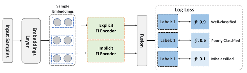
Figure 1: The workflow of current parallel-structured CTR models

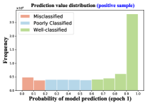
(a) Training on Frappe

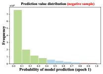
(b) Training on Frappe

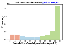
(c) Training on ML-tag

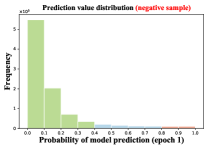
(d) Training on ML-tag

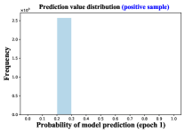
(e) Validation on Frappe

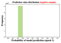
(f) Validation on Frappe

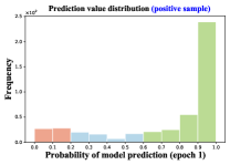
(g) Validation on ML-tag

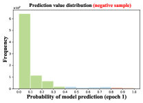
(h) Validation on ML-tag

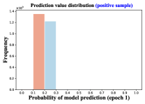
(i) Validation on Frappe

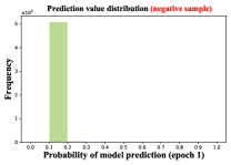
(j) Validation on Frappe

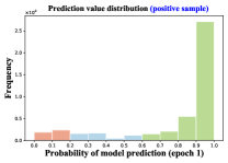
(k) Validation on ML-tag

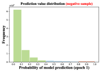
(l) Validation on ML-tag

Figure 2: Distribution of DNN’s prediction results for positive and negative samples on training and validation datasets. Red indicates misclassified, blue indicates poorly classified, and green indicates well-classified.

Compared to stacked structures, the CTR model with parallel structure has received considerable research attention due to their decoupled ability and parallel computing-friendly properties [7, 5, 18], leading to state-of-the-art (SOTA) performance [16, 19]. Despite the effectiveness of current CTR models based on this parallel structure, there are limitations to overcome:

• Insufficient sample differentiation ability. As shown in Figure 1, we classify the samples in terms of the gap between the model predictions and the labels as: #Well-classified (corresponding to easy sample, e.g., a male student purchasing a T-shirt during summer, aligning with typical behavior), #Poorly Classified (corresponding to challenging sample, e.g., a female student buys a T-shirt in winter, which seems unconventional but is explained by her spending a lot of time in warm indoor environments), and #Misclassified (corresponding to hard sample, e.g., a male engineer purchases lipstick, which is non-typical behavior for males). Most CTR models learn the above three classes of samples indiscriminately, without the ability to differentiate samples based on complexity or learning difficulty. Without this, models may overlook the informative hard samples essential for enhancing robustness and predictive accuracy [20].

• Unbalanced sample distribution. We visualize the distribution of the DNN’s prediction results during the initial learning phase, as illustrated in Figure 2. The CTR model fits most of the samples (i.e., more green part) quickly after the first epoch. However, multiple problems arise on the validation set: (1) Figure 2 (a $\sim$ d) reveals an obvious thing that there are significantly more easy samples than hard samples. This disproportionate influence of simple samples can limit a model’s effectiveness and its generalization capabilities [21]; (2) from Figure 2 (e) and (i), we can identify insufficient generalization on the Frappe dataset; (3) from Figure 2 (e $\sim$ l), the model does not fit hard and challenging samples well as the number of epochs increases.

• Undifferentiated learning process. The training process of most CTR models tends to use the same supervision signal for all encoders, ignoring the varying degree to which different samples contribute to the learning process. This can lead to poor encoder training that fails to adequately capture the more appropriate interaction information from different samples.

To address the aforementioned limitations, we introduce a novel CTR prediction framework, called the Twin Focus Framework for CTR (TF4CTR). Considering the excellent performance of parallel structures, we focus on applying our proposed framework within CTR models that utilize such structures, thereby helping various representative baseline models to differentiate sample complexity in a model-agnostic manner adaptively. This enables encoders to capture feature interaction information more effectively and target-specific. More specifically, this framework incorporates two plug-and-play modules alongside a target-specific loss function designed to enhance the model’s prediction and generalization capabilities: (1) Sample Selection Embedding Module (SSEM) aims to select different encoders for samples of different complexity, thus preventing the encoder from being simultaneously biased towards capturing information in simple samples. SSEM is positioned at the base of the model, and adaptively selects the most appropriate encoder for the current input sample; (2) Dynamic Fusion Module (DFM) dynamically aggregates and evaluates the outputs of different encoders to achieve a more accurate prediction outcome. In this way, it can take advantage of multiple encoding strategies to dynamically synthesize information to accommodate the diversity of input data; (3) Twin Focus (TF) Loss provides target-specific auxiliary supervision signals to encoders of varying complexities. It aims to refine the learning process by providing differentiated training signals that emphasize the learning of complex encoders to harder samples or simple encoders to easy samples, thus reducing the effect of the imbalance in the number of hard and easy samples and improving the overall generalization ability of the model. The major contributions of this paper are summarized as follows:

• We elucidate three inherent limitations of current parallel-structured CTR models and confirm their existence through experimental validation and theoretical analysis.

• We propose a novel model-agnostic CTR framework, called TF4CTR, which improves the information capture ability of the encoder and the final prediction accuracy of the model through adaptive sample differentiation.

• We introduce a lightweight Sample Selection Embedding Module, Dynamic Fusion Module, and Twin Focus Loss, all of which can be seamlessly integrated as plug-and-play components into various CTR baseline models to improve their generalization capabilities and performance.

• We conduct comprehensive experiments across five real-world datasets, demonstrating the effectiveness and compatibility of the proposed TF4CTR framework.

II Preliminaries

II-A CTR Prediction Task

CTR prediction is typically considered a binary classification task that utilizes user profiles [1, 22], item attributes, and context as features to predict the probability of a user clicking on an item. The composition of these three types of features is as follows:

• User profiles (p): age, gender, occupation, etc.

• Item attributes (a): brand, price, category, etc.

• Context (c): timestamp, device, position, etc.

Further, we can define a CTR sample in the tuple data format: $X=\{\textbf{p},\textbf{a},\textbf{c}\}$. Variable $y\in\{0,1\}$ is an true label for user click behavior:

$$y=\begin{cases}1,&\text{user}\text{ has clicked }\text{item},\\ 0,&\text{ otherwise. }\end{cases}$$ (1)

A positive sample when $y=1$ and a negative sample when $y=0$.

The final purpose of the CTR prediction model, which is to reduce the gap between the model’s prediction and the true label, is formulated as follows:

$${\arg\min}\|y-\hat{y}\|,$$ (2)

$$\hat{y}=\texttt{MODEL}(X).$$

where MODEL denotes the CTR model.

II-B Three Categories of Samples

In the real world, CTR prediction tasks handle millions of data points [15, 23] and encounter issues related to high sparsity and the cold start problem, with some datasets exhibiting sparsity levels exceeding 99.9% [22]. Consequently, the samples within these datasets inevitably present varied levels of prediction difficulty. Based on the discrepancies between the model’s predictions and the true labels, we can categorize these samples into three categories:

• #Well-classified $\leftrightarrow$ easy sample,

• #Poorly Classified $\leftrightarrow$ challenging sample,

• #Misclassified $\leftrightarrow$ hard sample.

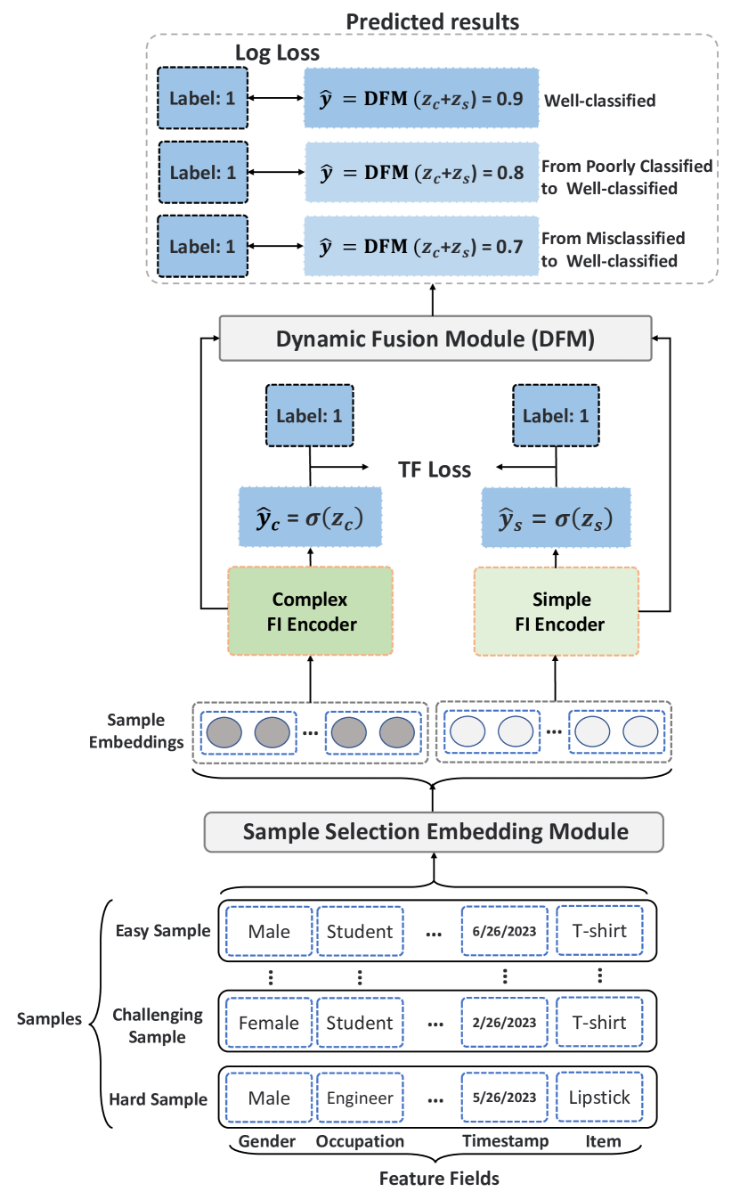
Figure 3: The workflow of TF4CTR.

III PROPOSED METHOD

III-A Twin Focus Networks Framework

Inspired by the Focal Loss [21], the TF4CTR framework introduces an adaptive strategy for differentiating between sample data. This allows for targeted learning of network parameters to predict CTR. As depicted in Figure 3, the architecture of TF4CTR is structured around four main components:

• Sample Selection Embedding Module (SSEM): This component adaptively differentiates the post-embedding samples, directing them to the most appropriate encoder. For instance, easy samples are channeled to a simple encoder, whereas hard samples are routed to a complex encoder. Challenging samples are determined collectively by multiple encoders.

• Differentiated Feature Interaction Encoder (FI Encoder): This encoder performs interactions on data samples to varying extents. Our proposed framework allows a variety of FI Encoders to achieve more precise predictions and enhance the model’s overall generalization capability. To keep it simple, we adopt the simple and widely-used Multilayer Perceptron (MLP) as our base FI Encoder. The depth of the MLP is used to differentiate between the complex and simple FI Encoders, thereby generating two distinct predictions for the same sample.

• Twin Focus Loss (TF Loss) Function: This loss function provides auxiliary supervision signals to the complex and simple FI Encoders. This encourages the encoders to target-specific learn the feature interactions of complex (or simple) samples.

• Dynamic Fusion Module (DFM): This module dynamically integrates the prediction results from the distinct FI Encoders to reduce classification errors.

We randomly sample a mini-batch of $N$ user click behaviors. As depicted in Figure 3, each sample within the batch contains several feature fields $f$, with each field comprising its own attributes. Taking an easy sample as an example, {Gender, Occupation, Timestamp, Item} $\in f$, we can extract the specific features of a click behavior: {Male, Student, 6/26/2023, T-shirt}. From the interpretability perspective, it makes sense for a male student to show interest in purchasing a T-shirt in summer, thus it is categorized as an easy sample ($es$). In contrast, for the features set {Male, Engineer, 5/26/2023, Lipstick}, this can be interpreted as a male engineer who suddenly decides to purchase lipstick in May, possibly as a gift. Because it is less typical for males to develop an interest in lipstick, this scenario would be classified as a hard sample ($hs$). For the challenging sample {Female, Student, 2/26/2023, T-shirt}, it is observed that a female student purchases a T-shirt during winter. Although buying a T-shirt in winter may seem unconventional, the reason for this purchase could be that she spends significant time in heated indoor environments. Therefore, to more accurately predict user click behavior, it is essential to analyze user data patterns further.

III-B Embedding Layer

In most deep learning-based CTR models, the embedding layer is an essential component [16, 18, 22]. Simply put, for each input sample $x_{i}\in X$ ($x_{i}$ denotes a particular feature of the input sample $X$), it can be transformed into a high-dimensional sparse vector using one-hot encoding [1, 24, 25], which is then converted into a low-dimensional dense embedding through the embedding matrix: $\mathbf{e}_{i}=E_{i}x_{i}$, where $E_{i}\in\mathbb{R}^{d\times s_{i}}$ and $s_{i}$ separately indicate the embedding matrix and the vocabulary size for the $i^{th}$ field, and $d$ represents the embedding dimension. After that, we concatenate the individual features to get the input $\mathbf{h}=\left[\mathbf{e}_{1},\mathbf{e}_{2},\cdots,\mathbf{e}_{f}\right]\in\mathbb{R}^{D}$ to the FI Encoder, where $D=\sum_{i=1}^{f}d$. However, it is often not a good choice to directly input $\mathbf{h}$ after the embedding layer into the FI Encoder, and the validity of this idea has been confirmed in many previous works [26, 19, 12, 13].

III-C Sample Selection Embedding Module

In this work, we start from the predictive difficulty of the samples themselves and use the SSEM to make an adaptive selection. This module is designed to evaluate the complexity of the samples and guide them to different encoders in the model architecture. For example, simple samples like the previously mentioned male student interested in a T-shirt may be processed through a simpler encoder that captures the most straightforward features, while hard samples like the male engineer interested in lipstick may require a more sophisticated encoder that can learn to understand deeper data patterns and feature interactions. This adaptive approach aims to optimize the model’s performance by ensuring that each sample is processed in an efficient and effective manner. By recognizing and treating samples differently based on their complexity, the SSEM contributes to an overall more accurate and robust CTR prediction model.

Specifically, we have defined several methods to implement the SSEM, as follows:

• Separate Embedding Representations (SER): Instead of sharing feature embeddings between different encoders [8], we use two distinct embedding matrices $\mathbf{E}_{es}$ and $\mathbf{E}_{hs}$ to embed the input sample $X$, which greatly alleviates the problem of excessive sharing [7]. Additionally, by changing the embedding dimensions, samples can obtain representations that are better suited to their complexity. This is formalized as:

  $$\mathbf{h}_{es}=\mathbf{E}_{es}X,\ \ \mathbf{h}_{hs}=\mathbf{E}_{hs}X,$$ (3)

  where $\mathbf{E}_{es}\in\mathbb{R}^{\frac{d}{2}\times s_{i}\times f}$ and $\mathbf{E}_{hs}\in\mathbb{R}^{d\times s_{i}\times f}$, $\mathbf{h}_{es}$ and $\mathbf{h}_{hs}$ denote easy sample embedding and hard sample embedding respectively.

• Gating Mechanism (GM): A simple yet effective gating network can serve as a judge to direct samples of varying difficulties to appropriate encoders. To reduce the number of model parameters, a single gating unit is utilized to control the input embeddings for FI Encoders:

  $$\mathrm{g} =\sigma(\texttt{Gate}(\mathbf{h})),$$ (4)

  $$\mathbf{h}_{es} =\mathrm{g}\cdot\mathbf{h},\ \ \mathbf{h}_{hs}=(1-\mathrm{g})\cdot\mathbf{h},$$

  where $\mathrm{g}\in\mathbb{R}^{1}$ is the gate value, $\sigma$ is the sigmoid function, $\cdot$ denotes the dot product, and Gate denotes a gating unit. For convenience, we implement this using a simple MLP, and other more complex gating networks could be used here.

• Multi-gate Mixture-of-Experts Structures (MMoE): To address the potential issue of insufficient sample differentiation capability with a gating unit alone, we further incorporate the concept of MMOE [27]. This approach allows multiple expert networks to evaluate the same sample and selects the most suitable FI Encoder for the sample using the gating mechanism. Considering the complexity, we only use two experts paired with their corresponding gating units:

  $$\mathrm{g}_{11},\mathrm{g}_{12} =\texttt{SoftMax}(\texttt{Gate}_{1}(\mathbf{h})),$$ (5)

  $$\mathrm{g}_{21},\mathrm{g}_{22} =\texttt{SoftMax}(\texttt{Gate}_{2}(\mathbf{h})),$$

  $$\mathrm{\textbf{m}_{1}} =\texttt{EX}_{1}(\mathbf{h}),$$

  $$\mathrm{\textbf{m}_{2}} =\texttt{EX}_{2}(\mathbf{h}),$$

  $$\mathbf{h}_{es} =\mathrm{{g}_{11}}\cdot\mathrm{\textbf{m}_{1}}+\mathrm{{g}_{12}}\cdot\mathrm{\textbf{m}_{2}},$$

  $$\mathbf{h}_{hs} =\mathrm{{g}_{21}}\cdot\mathrm{\textbf{m}_{1}}+\mathrm{{g}_{22}}\cdot\mathrm{\textbf{m}_{2}},$$

  where EX represents an expert network, $\mathrm{\textbf{m}}\in\mathbb{R}^{D}$ represents the output of the expert network.

III-D Differentiated FI Encoder

Improving the FI Encoder has always been a focal point of research in the CTR prediction [11, 5, 28, 29, 7]. Generally, FI Encoders can be categorized into two types based on their encoding methods: (1) explicit FI Encoders [22, 16] enhance the order of feature interactions according to predefined rules, thereby obtaining interpretable low-order feature interactions; (2) Implicit FI Encoders [18, 17] capture the interactions between features implicitly through the deep neural network. Most studies [8, 5, 16] suggest that combining explicit and implicit FI Encoders can further improve model performance. As a result, researchers are dedicated to designing various more complex explicit FI Encoders to enhance the overall predictive ability and interpretability of the model.

In this work, however, we categorize FI Encoders simply as either simple or complex encoders, allowing samples of varying prediction difficulty levels to have more suitable differentiated encoding pathways. To keep it simple, we use MLP with different numbers of layers to validate this idea.

$$\hat{\mathbf{h}}_{es} =\texttt{MLP}_{s}(\mathbf{h}_{es}),\ \ \hat{\mathbf{h}}_{hs}=\texttt{MLP}_{c}(\mathbf{h}_{hs}),$$ (6)

$$z_{s} =\mathbf{W}_{s}\hat{\mathbf{h}}_{es},\ \ z_{c}=\mathbf{W}_{c}\hat{\mathbf{h}}_{hs},$$

$$\hat{y}_{s} =\sigma(z_{s}),\ \ \hat{y}_{c}=\sigma(z_{c}),$$

where $\hat{\mathbf{h}}_{es}$ ($\hat{\mathbf{h}}_{hs}$) denotes the final representation of the encoder, the number of layers in $\texttt{MLP}_{s}$ is smaller than the number of layers in $\texttt{MLP}_{c}$, $\hat{y}_{e}$ and $\hat{y}_{c}$ denote the prediction results of the simple encoder ($\texttt{MLP}_{s}$) and complex encoder ($\texttt{MLP}_{c}$) respectively, $\mathbf{W}_{s}$ and $\mathbf{W}_{c}$ are the learned weights, and $z$ is the logit value. Other more complex or simpler FI Encoders could similarly be employed.

III-E Twin Focus Loss Function

Relying only on a single and undifferentiated loss function for specialized training of differentiated FI Encoders is undoubtedly inefficient, and introducing an auxiliary loss function is an effective strategy [15]. Therefore, we further add an auxiliary loss to the FI Encoders, which is designed to facilitate the learning of parameters by both simple FI Encoders and complex FI Encoders that are more favorable to their respective target sample classes. Doing so improves the model’s ability to specialize on samples with different levels of difficulty. More specifically, this loss function encourages the simple FI Encoder to better fit easy samples, while encouraging the complex FI Encoder to better fit hard samples, and for the challenged samples to be jointly determined by the two FI Encoders. The general form of TF Loss is shown below:

$$\mathcal{L}_{TF}=\alpha\mathcal{L}_{\text{simple}}\left(\hat{y}_{s},y\right)+(1-\alpha)\mathcal{L}_{\text{complex}}\left(\hat{y}_{c},y\right),$$ (7)

$$\mathcal{L}_{\text{simple}}(\hat{y}_{s},y)=-\frac{1}{N}\sum_{i=1}^{N}(c+\hat{y}_{s,i})^{\gamma}\log\left(\hat{y}_{s,i}\right),\ \ c\in[0,1]$$

$$\mathcal{L}_{\text{complex}}(\hat{y}_{c},y)=-\frac{1}{N}\sum_{i=1}^{N}(m-\hat{y}_{c,i})^{\gamma}\log\left(\hat{y}_{c,i}\right),\ \ m=2-c$$

where $\alpha$ controls the balance between the losses attributed to the simple and complex FI Encoders. The true label is denoted by $y$, while $c\in[0,1]$ and $m\in[1,2]$ are a pair of coefficients. The term $\gamma$ acts as a modulating factor and is typically selected from set $\{1,2,3\}$. These hyperparameters allow for the fine-tuning of the TF Loss, ensuring that it is suitably calibrated to the specific requirements of the sample difficulty being addressed. $\mathcal{L}_{TF}$ is visualized for several hyperparameters in Figure 4. Briefly, the hyperparameter $c$ (and its corresponding $m$) can be used as a threshold to divide the range of applicability of various prediction results, thereby adjusting the corresponding loss function crosspoints. $\gamma$ then further adjusts the size of the loss using the $c$ dividing result as a reference.

Intuitively, as illustrated in Figure 4, it is evident that a decrease in $c$ results in expanded applicability for #Misclassified samples, while simultaneously diminishing the scope for #Poorly classified and #Well-classified samples. Concurrently, as $\gamma$ increases, the loss corresponding to the #Misclassified range decreases for $\mathcal{L}_{simple}$, and the losses for #Poorly classified and #Well-classified samples increase. This means that $\mathcal{L}_{simple}$ guided FI Encoder will be more inclined to learn #Poorly classified and #Well-classified samples. Conversely, the opposite trend is observed for $\mathcal{L}_{complex}$. By manipulating the loss function in this manner, we enable it to exhibit differential sensitivity to various types of samples, thereby guiding the two distinct FI Encoders to refine their optimization process for the sample types they are inherently more proficient at handling. This approach helps to enhance the performance of the model and its ability to generalize to sophisticated samples.

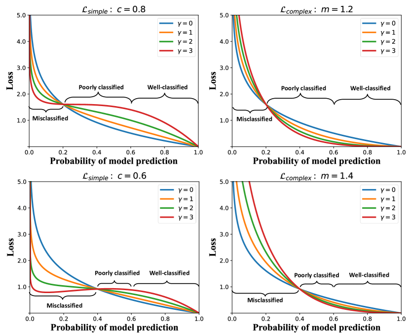
Figure 4: Visualization of $\mathcal{L}_{TF}$ for various hyperparameters

III-F Dynamic Fusion Module

We also tried various methods in order to dynamically converge more accurate predictions from different FI Encoders:

• Weighted Sum Fusion (WSF): This is a simple yet effective method that fusion the predictive outputs from differentiated encoders through a process of weighted summation:

  $$\hat{y}=\sigma(w_{1}z_{s}+w_{2}z_{c}),$$ (8)

  where $w_{1},w_{2}\in\mathbb{R}^{1}$ are a learnable parameter initialized to 0.5.

• Voting Fusion (VF): When we consider the process of fusion of the predicted results as a probabilistic choice, a voting mechanism [30] can be introduced naturally. However, to further tune the model’s predictions, we implement a tunable voting mechanism using Gumbel-Softmax [31] in the following form:

  $$\pi_{s} =\mathbf{W}_{es}\hat{\mathbf{h}}_{es},\ \ \pi_{c}=\mathbf{W}_{hs}\hat{\mathbf{h}}_{hs},$$ (9)

  $$p_{i} =\frac{\exp\left(\left(\log\left(\pi_{i}\right)+g_{i}\right)/\tau\right)}{\sum_{j=1}^{k}\exp\left(\left(\log\left(\pi_{j}\right)+g_{j}\right)/\tau\right)},$$

  $$\hat{y} =\sigma(p_{s}\cdot z_{s}+p_{c}\cdot z_{c}),$$

  where $p_{i}$ represents the probability of selecting $\pi_{i}\in\mathbb{R}^{1}$, $\tau$ represents the temperature coefficient, which controls the smoothness of the Gumbel-Softmax output, $g$ is i.i.d. sample drawn from Gumbel distribution. We can control the degree of certainty in the voting outcome by adjusting the temperature coefficient $\tau$. At lower values of $\tau$, the output approximates hard voting, selecting the option with the highest probability. Conversely, at higher values of $\tau$, the output becomes smoother, with probabilities across options more evenly distributed.

• Concatenation Fusion (CF): Concatenating the outputs of different FI Encoders and then passing them through a simple linear layer is also a simple and effective method, which is formulated as shown below:

  $$\hat{y}=\sigma\left(\mathbf{W}_{cf}\left[\hat{\mathbf{h}}_{es}\ ||\ \hat{\mathbf{h}}_{hs}\right]\right),$$ (10)

  where $\mathbf{W}_{cf}$ is learnable weight.

• Mixture-of-Experts Fusion (MoEF): Similar to SSEM, we can use Mixture-of-Experts networks to determine how much different encoders contribute to the final prediction result:

  $$\mathrm{g}_{1},\mathrm{g}_{2} =\texttt{SoftMax}(\texttt{gate}\left[\hat{\mathbf{h}}_{es}\ ||\ \hat{\mathbf{h}}_{hs}\right]),$$ (11)

  $$\mathrm{{m}_{1}} =\texttt{ex}_{1}(\left[\hat{\mathbf{h}}_{es}\ ||\ \hat{\mathbf{h}}_{hs}\right]),$$

  $$\mathrm{{m}_{2}} =\texttt{ex}_{2}(\left[\hat{\mathbf{h}}_{es}\ ||\ \hat{\mathbf{h}}_{hs}\right]),$$

  $$\hat{y} =\sigma(\mathrm{{g}_{1}}\cdot\mathrm{{m}_{1}}+\mathrm{{g}_{2}}\cdot\mathrm{{m}_{2}}),$$

  where $\mathrm{m}\in\mathbb{R}^{1}$, gate and ex denote micro gating units and expert networks, respectively.

III-G Multi-task Training

To integrate the TF4CTR framework into the CTR prediction scenario, we employ a multi-task training strategy to co-optimize the TF Loss and the original CTR prediction loss in an end-to-end manner. Thus, the final objective function can be expressed as:

$$\mathcal{L}_{total} =\mathcal{L}_{ctr}+\mathcal{L}_{TF},$$ (12)

where $\mathcal{L}_{ctr}=-\frac{1}{N}\sum_{i=1}^{N}\log\left(\hat{y}_{i}\right)$, $\hat{y}=(1-\hat{y})\ \text{if}\ y=0$, and $\hat{y}=\hat{y}\ \text{if}\ y=1$. To clearly delineate the overall workflow of the TF4CTR framework, we provide a detailed description of its complete training process, as shown in Algorithm 1.

Input: input samples $X\in N$;

Output: model parameters $\Theta$;

1 Initialize parameters $\Theta$;

2 while TF4CTR has not reached the early stopping patience threshold do

3       for $X\in N$ do

4             $\mathbf{h}_{es},\ \mathbf{h}_{hs}$ $\leftarrow$ SSEM($X$) according to Section III-C;

5             Get $\hat{y}_{s},\ \hat{y}_{c},z_{s},z_{c}$ from Differentiated FI Encoders according to Section III-D ;

6             $\hat{y}$ $\leftarrow$ DFM($z_{s},z_{c}$) according to Section III-F ;

7             Calculate Twin Focus Loss $\mathcal{L}_{TF}$ according to Eq. (7);

8             Calculate CTR Loss $\mathcal{L}_{ctr}$;

9             Get total loss according to Eq. (12);

10            

11       end for

12      Get Average gradients from mini-batch;

13       Update parameters by descending the gradients $\nabla_{\Theta}\mathcal{L}_{ctr}+\nabla_{\Theta}\mathcal{L}_{TF}$;

14 end while

return model parameters $\Theta$;

Algorithm 1 The training process of TF4CTR

Using the TF4CTR framework, Differentiated FI Encoders can be replaced by encoders from other models in line 5 of Algorithm 1.

III-H Theoretical Analysis

In most CTR models with parallel structures, a simple logical sum fusion method is widely favored [8, 22, 28], taking the form of $\hat{y}=\sigma(z_{s}+z_{c})$. To keep the formula derivation simple and understandable, we will use this form of fusion as a basis for deriving the gradients obtained for different types of samples.

III-H1 Gradient of $\mathcal{L}_{ctr}$ for Encoders

The gradient of $\mathcal{L}_{ctr}$ for logit values output by different encoders can be derived as:

$$\|\nabla_{(z_{s})}\mathcal{L}_{ctr}\| =\frac{\partial\left(\log\sigma(z_{s}+z_{c})\right)}{\partial z_{s}}=1-\sigma\left(z_{s}+z_{c}\right),$$ (13)

$$\|\nabla_{(z_{c})}\mathcal{L}_{ctr}\| =\frac{\partial\left(\log\sigma(z_{s}+z_{c})\right)}{\partial z_{c}}=1-\sigma\left(z_{s}+z_{c}\right).$$

This equation proves that $\mathcal{L}_{ctr}$ gives the same gradient for encoders with different task objectives. This often leads to untargeted learning of the encoders, thus weakening their performance and generalization ability.

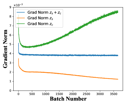
(a) $\mathcal{L}_{ctr}+\mathcal{L}_{TF}$

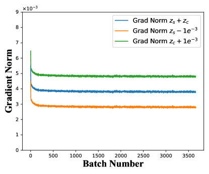
(b) $\mathcal{L}_{ctr}$ only

Figure 5: Gradient norm dynamics of $\mathcal{L}_{ctr}+\mathcal{L}_{TF}$ and $\mathcal{L}_{ctr}$ for the first training epoch on the Criteo dataset.

III-H2 Gradient of $\mathcal{L}_{TF}$ for Encoders

$$\|\nabla_{(z_{s})}\mathcal{L}_{simple}\| =\frac{\partial\left((c+\sigma(z_{s}))^{\gamma}\log\sigma(z_{s})\right)}{\partial z_{s}}$$ (14)

$$\propto(c+\sigma(z_{s}))^{\gamma-1}(1-\sigma(z_{s})),$$

$$\|\nabla_{(z_{c})}\mathcal{L}_{complex}\| =\frac{\partial\left((m-\sigma(z_{c}))^{\gamma}\log\sigma(z_{c})\right)}{\partial z_{c}}$$

$$\propto(m-\sigma(z_{c}))^{\gamma-1}(1-\sigma(z_{c})),$$

From this equation, it can be seen that $\mathcal{L}_{TF}$ can be tuned to the gradient size accepted by different encoders using the hyperparameters $c$ and $\gamma$. For example, when the simple encoder encounters a hard sample (i.e., the gap between the predicted value and the true label is too large), the $\sigma(z_{s})$ at this point tends to be a smaller value, which results in the value of $c+\sigma(z_{s})$ being less than 1. The $\gamma$ amplifies this deflated scale, thus the loss results in the simple encoder accepts a lower gradient from difficult samples, and the opposite for complex encoders. On the other hand, as shown in Figure 2, we weight the simple samples since they represent a larger proportion of the total samples, and the complete gradient of $\mathcal{L}_{TF}$ can be derived as:

$$\|\nabla_{(z_{s})}\mathcal{L}_{TF}\| \propto\alpha(c+\sigma(z_{s}))^{\gamma-1}(1-\sigma(z_{s})),$$ (15)

$$\|\nabla_{(z_{c})}\mathcal{L}_{TF}\| \propto(1-\alpha)(c+\sigma(z_{c}))^{\gamma-1}(1-\sigma(z_{c})).$$

In order to further demonstrate whether $\mathcal{L}_{TF}$ generates varying gradients for encoders, enabling them to precisely capture target-specific feature interaction information across different samples. We visualized the gradient norm obtained from logit values on the Criteo dataset, and the results are shown in Figure 5. In Figure 5 (a), benefiting from the addition of $\mathcal{L}_{TF}$, the logit $z_{c}$ of the complex encoder output is gradually increasing, while the logit $z_{s}$ of the simple encoder is gradually decreasing. This implies that after the model has quickly fitted the simple samples, it gradually emphasizes capturing more effective information from the complex samples. However, as shown in Figure 5 (b), $z_{c}$ and $z_{s}$ have no change in the gradient that they are subjected to as the number of batch increases. This implies that the model does not realize that it is only fitting the simple samples, which reduces the model performance.

IV EXPERIMENTS

In this section, we conduct extensive experiments on five real-world CTR prediction datasets to validate the effectiveness and compatibility of the proposed TF4CTR framework and address the following research questions (RQs):

• RQ1 Can the proposed TF Loss be generalized across different models? Moreover, does it outperform similar loss functions?

• RQ2 Do the proposed SSEM and DFM synergistically enhance model performance when combined? Which combination is the highest for performance improvement?

• RQ3 Does our proposed model framework exhibit superiority over other models or frameworks?

• RQ4 Does the TF4CTR framework generalize better than other representative baseline models?

• RQ5 How should the hyperparameters of TF Loss be configured and balanced?

• RQ6 Is the TF4CTR framework lightweight and does it improve the generalization of the model?

IV-A Experimental Settings

Datasets and preprocessing. We evaluate TF4CTR on five real-world datasets: Criteo [1], KKBox [2], ML-1M [22], ML-tag [11] [2], and Frappe [11, 32]. Table I provides detailed information about these datasets. A more detailed description of these datasets can be found in the given references and links.

For data preprocessing methods, we follow to the protocols established by [1]. Notably, due to the Criteo dataset’s large size and extremely high sparsity (over 99.99%) [22], we implement a threshold of 10, replacing features occurring less than this threshold with a default ”OOV” token. For other datasets, a threshold of 2 is applied. Meanwhile, on the Criteo dataset, we discretize numerical features by rounding down each numeric value $x$ to $\lfloor\log^{2}(x)\rfloor$ for $x>2$, and setting $x=1$ otherwise, following the approach used by the winner of the Criteo competition.

TABLE I: Dataset statistics

Dataset	#Instances	#Fields	#Features	#Split
Criteo	45,840,617	39	5,549,252	8:1:1
KKBox	7,377,418	13	227,853	8:1:1
ML-1M	1,006,209	5	9,626	8:1:1
ML-tag	2,006,859	3	88,596	7:2:1
Frappe	288,609	10	5,382	7:2:1

TABLE II: Compatibility study of TF Loss. $\triangle\text{AUC}$ denote the absolute performance improvement. AVG.AUC and AVG.RI denotes the average AUC performance and average absolute improvement on the four datasets, respectively. Typically, CTR researchers consider an improvement of 0.1% in AUC to be statistically significant [17, 1].

FI Encoder				Base Model	Loss function	KKBox		Criteo		ML-tag		Frappe	AVG.AUC	AVG.RI
			AUC(%)$\uparrow$	$\triangle\text{AUC}\uparrow$	AUC(%)$\uparrow$	$\triangle\text{AUC}\uparrow$	AUC(%)$\uparrow$	$\triangle\text{AUC}\uparrow$	AUC(%)$\uparrow$	$\triangle\text{AUC}\uparrow$
MLP	DualMLP	Log Loss (Base)	84.08	-	81.40	-	96.96	-	98.37	-	90.20	-
		Focal Loss [21]	83.83	-0.25	81.42	+0.02	96.99	+0.03	98.29	-0.08	90.13	-0.07
		R-CE Loss [33]	84.20	+0.12	81.36	-0.04	97.07	+0.11	98.35	-0.02	90.24	+0.04
		TF Loss (Ours)	84.29	+0.21	81.48	+0.08	97.12	+0.16	98.55	+0.18	90.36	+0.16
Attention	AutoInt+	Log Loss (Base)	84.08	-	81.39	-	96.97	-	98.41	-	90.21	-
		Focal Loss [21]	83.91	-0.17	81.35	-0.04	96.76	-0.21	98.53	+0.12	90.13	-0.08
		R-CE Loss [33]	84.01	-0.07	81.40	+0.01	97.08	+0.11	98.46	+0.05	90.23	+0.02
		TF Loss (Ours)	84.25	+0.17	81.46	+0.07	97.11	+0.14	98.56	+0.15	90.34	+0.13
Product	DeepFM	Log Loss (Base)	84.11	-	81.38	-	96.92	-	98.37	-	90.19	-
		Focal Loss [21]	83.81	-0.30	81.33	-0.05	96.95	+0.03	98.43	+0.06	90.13	-0.06
		R-CE Loss [33]	84.11	+0.00	81.41	+0.03	96.92	+0.00	98.42	+0.05	90.21	+0.02
		TF Loss (Ours)	84.31	+0.20	81.43	+0.05	96.99	+0.07	98.48	+0.11	90.30	+0.11
	DCN	Log Loss (Base)	84.22	-	81.39	-	96.91	-	98.38	-	90.22	-
		Focal Loss [21]	84.07	-0.15	81.38	-0.01	96.85	-0.06	98.46	+0.08	90.19	-0.03
		R-CE Loss [33]	84.00	-0.22	81.32	-0.07	97.10	+0.19	98.39	+0.01	90.20	+0.02
		TF Loss (Ours)	84.35	+0.13	81.44	+0.05	97.12	+0.21	98.53	+0.15	90.36	+0.14
	DCNv2	Log Loss (Base)	84.24	-	81.40	-	96.92	-	98.45	-	90.25	-
		Focal Loss [21]	83.86	-0.38	81.42	+0.02	96.99	+0.07	98.50	+0.05	90.19	-0.06
		R-CE Loss [33]	84.18	-0.06	81.40	+0.00	96.90	-0.02	98.46	+0.01	90.23	-0.02
		TF Loss (Ours)	84.32	+0.08	81.45	+0.05	97.03	+0.11	98.52	+0.07	90.33	+0.08
	AFN+	Log Loss (Base)	83.57	-	81.31	-	96.84	-	98.19	-	89.97	-
		Focal Loss [21]	82.92	-0.65	81.25	-0.06	96.43	-0.41	97.79	-0.40	89.59	-0.38
		R-CE Loss [33]	83.74	+0.17	81.31	+0.00	96.88	+0.04	98.20	+0.01	90.03	+0.06
		TF Loss (Ours)	84.37	+0.80	81.42	+0.11	97.02	+0.18	98.45	+0.26	90.31	+0.34

Evaluation metrics. To compare the performance, we utilize two commonly used metrics in CTR models: AUC, gAUC [22, 16, 34]. AUC stands for Area Under the ROC Curve, which measures the probability that a positive instance will be ranked higher than a randomly chosen negative one. gAUC implements user-level AUC computation. It is worth noting that even a slight improvement (e.g., 0.1%) in AUC and gAUC is meaningful in the context of CTR prediction tasks [7, 17, 1].

Baselines. We compared TF4CTR with some state-of-the-art (SOTA) models (+ denotes Integrating the original model with DNN networks):

• Focal Loss [21]: It is designed to address class imbalance by focusing more on hard-to-classify samples.

• R-CE Loss [33]: This treats some of the hard samples as outliers and prevents the model from learning the wrong information to improve the performance of the model.

• Wide & Deep [6]: It consists of logistic regression (Wide) and feedforward neural network (Deep) integration.

• DeepFM [8]: This model combines parallelly FM with feedforward neural networks by sharing embeddings.

• DCN [9]: This model proposes a CrossNet that can explicitly model feature interactions and integrates feedforward neural networks in parallel.

• xDeepFM [28]: This model is similar to DCN, and its proposed compressed interaction network (CIN) improves the level of feature interaction from bit-wise to vector-wise.

• AutoInt+ [22]: This model learns higher-order feature interactions for the first time using a multi-headed attention mechanism.

• AFN+ [11]: This model uses a logarithmic transformation layer to learn feature interactions of adaptive order.

• DCNv2 [5]: This model expands the dimensionality of the projection matrix based on DCN and introduces a mixture of low-rank expert systems to optimize the model inference speed.

• EDCN [7]: This model attempts to introduce a plug-and-play Bridge Module and Regulation Module for DCNs to mitigate the gradient vanishing problem and improve the model performance.

• CL4CTR [17]: This is a CTR prediction model based on contrast learning. Its aim is to adopt a self-supervised approach to the environmental data sparsity problem.

• EulerNet [29]: It utilizes a rigorous Eulerian formulation to adaptively capture feature interaction information.

Implementation Details. We implement all models using PyTorch [35] and refer to existing works [1, 36]. We employ the Adam optimizer [37] to optimize all models, with a default learning rate set to 0.001. For the sake of fair comparison, we set the embedding dimension to 16 [1, 2], the numbers of MLP hidden units are [400, 400, 400]. The batch size is set to 4,096 on the Criteo dataset and 10,000 on the other datasets. To prevent overfitting, we employ early stopping with a patience value of 2. The hyperparameters of the baseline model are configured and finetuned based on the optimal values provided in [36, 1] and their original paper. Further details on model hyperparameters and dataset configurations are available in our straightforward and accessible running logs, and are not reiterated here.

IV-B Effectiveness Analysis

IV-B1 Comparison and Compatibility Study of Loss (RQ1)

To verify whether our proposed $\mathcal{L}_{TF}$ can be generalized to other SOTA models and outperform other loss functions, we fix the hyperparameters of the base model and conduct compatibility and comparison experiments. The results are shown in Table II. We bold the best performance, while underlined scores are the second best.

We can find that TF Loss gains performance on all four datasets relative to the base Logloss. This proves that the model optimized by TF Loss has better generalization ability and performance. It is worth mentioning that the AFN+ model does not perform well with Logloss optimization, but after optimization with TF Loss, the model achieves the same benchmarks as the other SOTA models, and even achieves the best performance on the KKBox dataset. Additionally, the design idea of TF Loss is to help encoders target-specific handling samples of varying difficulty, thereby enabling more precise adjustment of model parameters.

Meanwhile, we further compared the performance differences when optimizing models with TF Loss and other loss functions. R-CE Loss often achieves the sub-optimal performance, while Focal Loss is not always effective, and often even degrades the performance of the model. We empirically think that this is due to the loss weights of Focal Loss always being less than 1, leading to a less effective supervision signal received by the encoders. Regarding R-CE Loss, it abandons the optimization of hard samples, thereby allowing the model to focus more on the information within challenging and easy samples. However, this approach is not always effective. For instance, in DCNv2, R-CE Loss led to negative optimization and recent work [38] suggests that encouraging the model to learn simpler samples might lead to gradient vanishing issues. For TF Loss, its effectiveness in enhancing model performance across various datasets and models further confirms the validity of our approach.

TABLE III: Performance comparison of different SSEM and DFM methods. Bold indicates the best-combined performance.

ML-tag			Method	WSF		VF		CF		MoEF		Sum		Frappe	Method	WSF		VF		CF		MoEF		Sum
		AUC	gAUC	AUC	gAUC	AUC	gAUC	AUC	gAUC	AUC	gAUC			AUC	gAUC	AUC	gAUC	AUC	gAUC	AUC	gAUC	AUC	gAUC
	SER	97.46	96.50	96.96	96.02	97.25	96.33	97.23	96.26	97.44	96.50		SER	98.72	98.17	98.52	98.02	98.70	98.21	98.64	98.20	98.72	98.21
	GM	97.02	96.07	97.02	96.09	97.02	96.07	96.99	95.99	97.09	96.19		GM	98.57	98.06	98.40	97.88	98.41	97.84	98.42	97.92	98.57	97.97
	MoE	96.79	95.72	96.95	95.94	96.82	95.79	96.77	95.72	96.79	95.77		MoE	98.54	98.00	98.53	98.00	98.56	98.01	98.44	9791	98.55	97.97
	Share	97.06	96.18	97.04	96.12	97.03	96.05	97.00	95.98	97.11	96.19		Share	98.52	98.02	98.51	97.98	98.54	98.04	98.41	97.85	98.51	97.98
KKBox	Method	WSF		VF		CF		MoEF		Sum		ML-1M	Method	WSF		VF		CF		MoEF		Sum
		AUC	gAUC	AUC	gAUC	AUC	gAUC	AUC	gAUC	AUC	gAUC			AUC	gAUC	AUC	gAUC	AUC	gAUC	AUC	gAUC	AUC	gAUC
	SER	84.47	77.60	84.17	77.11	84.36	77.48	84.50	77.62	84.41	77.54		SER	81.94	77.50	81.57	77.01	81.32	76.79	81.46	76.73	81.83	77.39
	GM	83.92	76.82	83.78	76.60	83.98	76.95	83.97	76.88	83.97	77.00		GM	81.61	76.88	81.27	76.45	81.36	77.01	81.24	76.58	81.41	76.76
	MoE	83.71	76.53	83.59	76.27	83.73	76.51	83.75	76.63	83.76	76.52		MoE	81.27	76.56	81.26	76.42	81.29	76.55	81.31	76.74	81.19	76.39
	Share	84.05	77.03	83.83	76.66	84.11	77.07	84.08	77.07	84.09	77.17		Share	81.58	77.05	81.33	76.52	81.41	77.00	81.35	76.95	81.26	76.69

TABLE IV: Performance comparison of different models. We conducted a two-tailed T-test ($p$-values) to assess the statistical significance between the TF4CTR and the best baseline model.

Dataset			Metric	WideDeep	DeepFM	DCN	xDeepFM	AutoInt+	AFN+	DCNv2	EDCN	CL4CTR	EulerNet	TF4CTR	$p$-values
KKBox	$\text{AUC(\%)}\uparrow$	84.12	84.11	84.22	84.02	84.08	83.57	84.24	83.96	84.05	83.68	$\mathbf{84.50}$	2.44e-4
ML-1M	$\text{AUC(\%)}\uparrow$	81.22	81.37	81.38	81.37	81.30	81.37	81.44	81.22	81.13	81.45	$\mathbf{81.94}$	4.79e-4
ML-tag	$\text{AUC(\%)}\uparrow$	96.92	96.92	96.91	96.92	96.97	96.84	96.92	96.03	96.83	96.79	$\mathbf{97.46}$	1.49e-4
Frappe	$\text{AUC(\%)}\uparrow$	98.32	98.37	98.38	98.45	98.41	98.19	98.45	98.41	98.27	98.16	$\mathbf{98.72}$	7.26e-5
Criteo	$\text{AUC(\%)}\uparrow$	81.38	81.38	81.39	81.40	81.39	81.31	81.40	81.39	81.36	81.37	$\mathbf{81.50}$	4.29e-5

IV-B2 Comparison and Combination Study of SSEM and DFM Method (RQ2)

To validate which implementations of SSEM and DFM are more effective, we conducted experiments with a fixed $\alpha=0.25$ and a 3-layer $\texttt{MLP}_{c}$, as shown in Table III. Share means that instead of using SSEM, different encoders are allowed to share the same feature embedding, and Sum means that the logit values output by the encoders are subjected to a simple summing operation to obtain the final model prediction. We can draw several findings from the results:

• The SER method demonstrated superior performance across all four datasets. This proves the validity of the SSEM model. Empirically, we attribute this to its ability to further decouple the embedding representation learning process of samples, allowing for gradients to propagate back without mutual interference.

• Sophisticated fusion methodologies do not guarantee superior effectiveness; conversely, the simpler WSF and Sum methods can also yield enhanced performance. For instance, the WSF approach demonstrated exceptional results on the ML-tag, Frappe, and ML-1M datasets, substantiating the effectiveness of the DFM. Notably, WSF introduces a minimal computational overhead with only two additional parameters compared to the Sum method, and yet, it achieves a performance increment of 0.1% on the ML-1M dataset.

• Certain integrations of SSEM and DFM yielded inferior results compared to the Share+Sum approach, exemplified by the MoE+VF combination on the ML-tag dataset and the GM+CF pairing on the KKBox dataset. However, on the Frappe and ML-1M datasets, these same combinations exhibited improvements over Share+Sum. We empirically consider that differences in the data distributions are the primary cause of this discrepancy. ML-tag and KKBox datasets are larger with more severe data distribution bias [39], whereas Frappe and ML-1M have smaller data volumes and simpler data distributions.

• The majority of SSEM+DFM pairings surpass the performance of Share+Sum. The optimal SSEM and DFM implementations outperform Share+Sum, achieving gains of 0.35% in AUC and 0.31% in gAUC on ML-tag, 0.21% in AUC and 0.19% in gAUC on Frappe, 0.41% in AUC and 0.45% in gAUC on KKBox, and 0.68% in AUC and 0.81% in gAUC on ML-1M. These results prove the effectiveness of our proposed SSEM and DFM.

IV-B3 Performance Comparison with Other Models (RQ3)

To further validate the outstanding performance of our proposed TF4CTR, we compare it against ten representative baseline models. Bold and underlined numbers respectively indicate the best and second-best results. Additionally, we conduct five runs of TF4CTR and the second-best baseline, and calculate the corresponding $p$-values. Based on the results as shown in Table IV, we can make the following observations:

• In smaller datasets such as ML-1M and Frappe, the performance gap among the ten selected representative baseline models is considerable, reaching up to 0.3%. However, in the larger Criteo dataset, this gap narrows. We empirically believe that the larger scale of data typically aids models in more consistently learning the underlying data distribution, which reduces the variance in performance between models. With large datasets, even simple models are capable of learning complex feature representations due to the extensive data available. In contrast, within smaller datasets, the complexity of the models and their regularization strategies may significantly influence performance. Therefore, model selection and tuning strategies should be appropriately adapted to the scale of the dataset to achieve optimal performance.

• Upon analyzing Tables II and IV, it is evident that TF4CTR consistently exhibits significant performance improvements over DualMLP. TF4CTR achieves an average AUC of 90.54% across the KKBOX, Criteo, ML-tag, and Frappe datasets. Compared to DualMLP optimized with Log Loss, TF4CTR realizes an absolute enhancement of 0.34%, affirming the overall effectiveness of our proposed framework. Furthermore, even against DualMLP optimized with TF Loss, our model still achieves an additional absolute gain of 0.18%. This further validates the effectiveness of our proposed SSEM and DFM, which help the model to better adapt to the auxiliary supervision signals provided by TF Loss, thereby enhancing the model’s performance and generalization capabilities.

  TABLE V: Compatibility study of TF4CTR.

  Model		ML-tag		Frappe		ML-1M
  	$\text{AUC(\%)}\uparrow$	$\triangle\text{AUC}\uparrow$	$\text{AUC(\%)}\uparrow$	$\triangle\text{AUC}\uparrow$	$\text{AUC(\%)}\uparrow$	$\triangle\text{AUC}\uparrow$
  DeepFM	96.92	-	98.37	-	81.37	-
  $\text{DeepFM}_{\text{TF4CTR}}$	97.03	0.11%	98.54	0.17%	81.56	0.19%
  WideDeep	96.92	-	98.32	-	81.22	-
  $\text{WideDeep}_{\text{TF4CTR}}$	96.99	0.07%	98.49	0.17%	81.63	0.41%
  xDeepFM	96.92	-	98.45	-	81.37	-
  $\text{xDeepFM}_{\text{TF4CTR}}$	97.03	0.11%	98.53	0.08%	81.65	0.28%

  

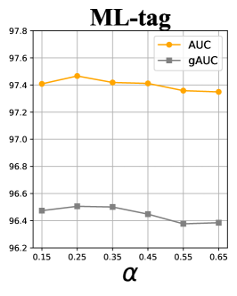
  (a)

  

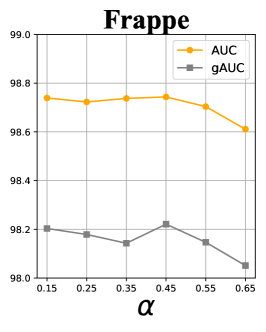
  (b)

  

  (c)

  Figure 6: Influence of magnitude $\alpha$ of $\mathcal{L}_{TF}$.

  

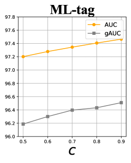
  (a)

  

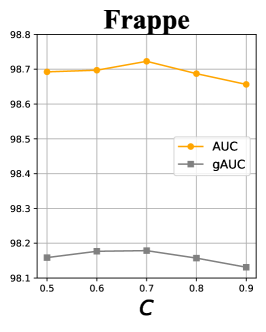
  (b)

  

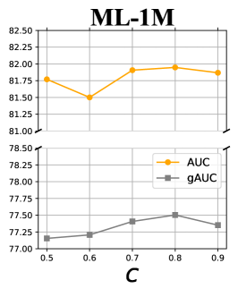
  (c)

  Figure 7: Influence of magnitude $c$ of $\mathcal{L}_{TF}$.

  

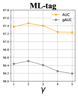
  (a)

  

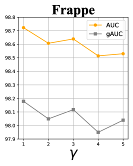
  (b)

  

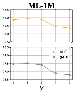
  (c)

  Figure 8: Influence of magnitude $\gamma$ of $\mathcal{L}_{TF}$.

  

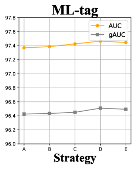
  (a)

  

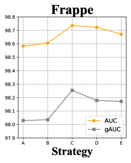
  (b)

  

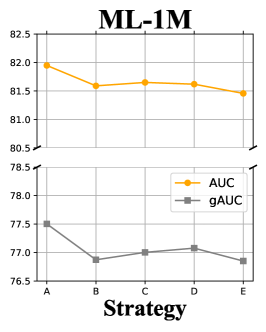
  (c)

  Figure 9: Influence of $\texttt{MLP}_{s}$.

• TF4CTR consistently achieves superior performance across five datasets. Compared to the second-best model on each dataset, it secures performance gains of 0.26% on KKBox, 0.49% on ML-1M, 0.49% on ML-tag, 0.27% on Frappe, and 0.1% on Criteo, all exceeding the significant improvement benchmark of 0.1%. Furthermore, two-tailed T-tests comparing TF4CTR with the second-best models yield $p$-values below 0.01 [16], indicating that the performance enhancements offered by our model are statistically significant.

IV-B4 Compatibility Study of TF4CTR (RQ4)

The TF4CTR framework proposed serves as a model-agnostic framework designed to enhance the performance of CTR models. To verify the compatibility of TF4CTR, it has been implemented into three benchmark baseline models, with experimental results detailed in Table V. The framework consistently enhances performance across multiple datasets. Notably, the WideDeep model achieves a performance increase of 0.41% on the ML-1M dataset, elevating its rank from the second to last to the top-2 position in Table IV. In addition, both DeepFM and xDeepFM models exhibited performance improvements, with most $\triangle\text{AUC}$ values exceeding 0.1%. These results substantiate the compatibility and effectiveness of the TF4CTR framework, underscoring its capacity to boost model performance across a spectrum of data environments consistently.

IV-C Hyper-parameter Analysis (RQ5)

In this section, we further investigate the effects that the three important parameters of TF Loss bring to the model. Here we fix the experimental setup of Section IV-B3 and change only the parameter to be studied.

IV-C1 Impact of $\alpha$

We fix the other hyperparameters and adjust $\alpha$ in the range [0.15, 0.65] in steps of 0.1, and the experimental results are shown in Figure 6. It can be observed that the model performance has a tendency to decrease as $\alpha$ increases and it reaches its optimal value at $\alpha=0.25$ on ML-tag, $\alpha=0.45$ on Frappe, and $\alpha=0.35$ on ML-1M. This further supports the idea that simple samples have a heavier portion in the dataset. We can make $\mathcal{L}_{TF}$ more adaptable to the sample distribution in the dataset by fine-grained adjustment of $\alpha$.

IV-C2 Impact of $c$

We introduce $c$ for $\mathcal{L}_{TF}$ aiming to use it as a threshold to classify #Misclassified, #Poorly Classified, and #Well-classified, thus further increasing or reducing the corresponding sample loss. The experimental results are shown in Figure 7, where the model performance on ML-tag increases with $c$, which indicates a narrower distribution of difficult samples on ML-tag. On Frappe and ML-1M, the peak is reached when $c$ is 0.7 and 0.8, and then starts to decrease. This suggests that the distribution of difficult samples is not the same in different datasets, and we can further adjust $c$ to maximize the gain of $\mathcal{L}_{TF}$ for performance.

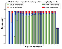
(a) Positive sample on Frappe

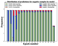
(b) Negative sample on Frappe

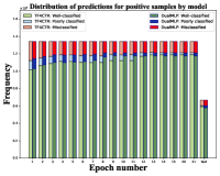
(c) Positive sample on ML-tag

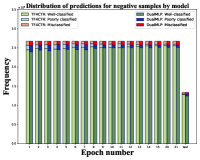
(d) Negative sample on ML-tag

Figure 10: Visualization of the model’s ability to generalize for samples of varying degrees of difficulty.

IV-C3 Impact of $\gamma$

We introduce the modulating factor $\gamma$ for $\mathcal{L}_{TF}$ in order to control the strength of the rescaling loss, i.e., the larger $\gamma$ is, the more extreme the loss function is. We fixed the rest of the parameters and adjust $\gamma$ in {1, 2, 3, 4, 5}, and the experimental results are shown in Figure 8. It can be observed that as $\gamma$ increases, there is an overall trend of decreasing performance of the model, so it is not a good idea to make the losses more extreme. We think that the main reason for the decrease in performance is that as $\gamma$ increases, $\mathcal{L}_{\text{complex}}$ focuses too much on hard samples, which leads to Challenging Sample being only learned in Simple FI Encoder, hence degrades the model’s performance. Meanwhile, it can be found that the model always achieves better performance when $\gamma$ is in {1, 2, 3}. Therefore, we propose to find a suitable $\gamma$ in this range.

IV-C4 Impact of $\texttt{MLP}_{s}$

To investigate the performance benefits provided by the simple encoder implemented with MLP across various neuron counts and layer configurations, we designed five structures:

• A: [400] uses a single linear layer with 400 neurons as a simple encoder.

• B: [800] employs a single linear layer with 800 neurons as a simple encoder.

• C: [200, 200] utilizes an MLP with two layers, each containing 200 neurons, as a simple encoder.

• D: [400, 400] uses an MLP with two layers, each containing 400 neurons, as a simple encoder.

• E: [800, 800] employs an MLP with two layers, each containing 800 neurons, as a simple encoder.

Experimental results, as shown in Figure 9, indicate that the optimal structure varies due to different distributions of sample difficulty within each dataset. Structure D achieves the best performance on the ML-tag dataset, while structure C peaks on Frappe, and structure A excels on ML-1M. From these observations, we can infer that ML-tag has fewer simple samples, followed by Frappe, and ML-1M has the least challenging samples. Additionally, it is evident that having a higher number of neurons does not necessarily improve the performance of a simple encoder, despite having the most parameters, structure E does not perform well across the three datasets.

IV-D Model Learning Process Investigation (RQ6)

IV-D1 Model Generalization across Learning Stages

To further confirm whether our method has aided DualMLP in better differentiating samples during the learning process, we adjust only the parameter early_stop_patience to ensure that both models had a consistent number of training epochs. Subsequently, we categorize the prediction outcomes on validation and test sets into three types using the thresholds {0.3, 0.6}: #Misclassified, #Poorly classified, and #Well-classified. After that, These categories are visualized in a bar chart, illustrating the models’ generalization capabilities on the validation set and their performance on the test set, as shown in Figure 10.

Overall, TF4CTR has a higher count of #Well-classified instances than DualMLP, both on the validation and test sets. Moreover, a significant reduction in the number of #Poorly classified instances is clearly observed. This further validates the effectiveness of the coordinated action of SSEM, DFM, and TF Loss within the TF4CTR framework, which enables the backbone model to better distinguish challenging samples, thereby enhancing the model’s performance. On the other hand, it is evident from the Frappe and ML-tag datasets that the performance of DualMLP stabilizes after the model has been trained to epoch 6 and epoch 8, respectively. In contrast, TF4CTR continues to refine its classification results, reducing the numbers of #Misclassified and #Poorly classified instances. The effectiveness of this refinement approach is further confirmed by the classification outcomes on the test set. Additionally, it is also worth mentioning that we can clearly observe that the model’s ability to classify positive samples is much lower than that for negative samples, which can be attributed to the imbalance of positive and negative samples within the dataset [38].

IV-D2 Running Time Comparison

To investigate the additional training cost introduced by our proposed plug-and-play modules—SSEM and DFM—and the TF Loss, we report the training time for the first epoch and the inference time on the validation set. The experimental results depicted in Table VI are collected on an Intel(R) Xeon(R) Platinum 8336C CPU and an NVIDIA GeForce RTX 4090 GPU.

TABLE VI: Training and inference time comparison for the first epoch on the KKBox dataset. x denotes the times compared to the base model.

Model		Training time (s)	Relative ratio	Inference time (s)	Relative ratio
DNN (Base)	23	-	3	-
xDeepFM	35	1.52x	4	1.33x
AutoInt+	36	1.56x	4	1.33x
AFN+	33	1.43x	4	1.33x
CL4CTR	63	2.73x	3	1x
DualMLP	25	1.08x	3	1x
TF4CTR (SER+MoEF)	30	1.30x	3	1x

As Table VI shows, we calculate the additional time complexity of various models in comparison to a simple DNN benchmark. It is observed that CL4CTR, due to its contrastive loss function tailored for embeddings, incurs the highest training time, yet its inference speed remains on par with the DNN. Models such as xDeepFM, AutoInt+, and AFN+ experience greater latencies in both training and inference times due to their more complex explicit encoders. With its excellent parallelization capabilities, DualMLP shows negligible difference in inference time compared to the DNN, and only a modest 1.08x increase in training time. TF4CTR and DualMLP have similar inference times, with a mere 0.22x difference in training time, and the significant performance improvement that the former provides over the latter has been thoroughly validated in previous sections. Consequently, the incremental model training time and inference latency associated with TF4CTR are deemed acceptable, confirming that the additional modules and loss function we introduced are lightweight and can be effectively applied in practical industrial settings.

V RELATED WORK

V-A Deep CTR Prediction

Most existing deep CTR models can be categorized into two types. (1) User behavior sequence-based CTR prediction models [14, 15, 40, 23, 41], which focus on modeling historical sequence data at the user level, such as past clicks, browsing, or purchase records. These models understand and predict future user actions, such as the likelihood of clicking on specific ads or purchasing products. (2) Feature interaction-based CTR prediction models [42, 43, 44, 7, 5, 13, 45, 24, 16], which have broader applicability and focus on the interactions among sample features. By identifying feature combinations that significantly affect the click-through rate, these models reveal deeper data patterns. Many CTR models with parallel structures achieve excellent performance [16, 19, 5], primarily due to their ability to integrate various structured feature encoders while maintaining efficient computational performance during feature processing and learning. These models typically employ deep learning techniques to automatically learn complex interactions between features, eliminating the need for manual feature engineering, and thereby enhancing the models’ generalization capabilities and predictive accuracy. For instance, attention-based models such as AFM [46], AutoInt [22], and FRNet [47] utilize attention mechanisms to find appropriate interaction orders among features, thereby filtering out noise and enhancing model performance. On the other hand, given the challenges MLPs face in capturing explicit low-order feature interactions [48], product-based models like DeepFM [8], DCNv2 [5], and GDCN [16] leverage the interpretability and reliability of explicit feature encoders to overcome the performance limitations of MLPs. Recent studies also indicate that DualMLP’s performance is not as poor as previously thought [18][19], suggesting that appropriate structural adjustments to MLPs can also yield significant improvements.

V-B Loss Function for CTR Prediction

CTR models aim to predict whether a user will click on a current item, thus categorizing this predictive behavior as a binary classification task. Typically, CTR prediction models employ binary cross-entropy (Log Loss) as the loss function [24, 18, 5], which optimizes each prediction outcome individually, thereby directly enhancing the accuracy of each model prediction. On the other hand, some studies [49, 50] acknowledge that the primary goal of CTR prediction is to ensure that the scores of positive samples exceed those of negative ones. Consequently, these studies attempt to combine pairwise rank loss and listwise loss with Log Loss in a joint training approach, thereby improving the model’s ranking capabilities.

With the rise of contrastive learning [51, 52], contrastive loss has also been increasingly applied to CTR prediction, such as in CL4CTR [17], which introduces concepts of feature alignment and uniformity across fields. However, the proposed contrastive module significantly increases training costs. CETN [25] introduces concepts of diversity and homogeneity in feature representation, adaptively adjusting the learning process of multiple encoders through the synergy of Do-InfoNCE and cosine loss. In the field of computer vision, Focal Loss [21] initially addresses the issue of imbalanced sample difficulty by adding a modulating factor to Log Loss. However, because this factor is always less than one, it may reduce the impact of vital supervision signals. Further, R-CE Loss [33] suggests disregarding outliers in the dataset to enhance data credibility, which aids the model in learning accurate feature representations.

VI Conclusion

In this paper, we analyze and identify the inherent limitations of current parallel-structured CTR prediction models, namely their lack of sample differentiation ability, unbalanced sample distribution, and undifferentiated learning process. To address these limitations, we propose the lightweight and plug-and-play Sample Selection Embedding Module, Dynamic Fusion Module, and Twin Focus Loss to form a model-agnostic CTR framework, TF4CTR. These three additional plug-ins can play roles in three positions of the feature interaction encoder’s input, output, and gradient optimization, respectively, to improve the generalization ability and performance of the model. The extensive experiments on five real-world datasets demonstrate the effectiveness and compatibility of the TF4CTR framework.

Honghao Li received the Bachelor degree in Computer engineering and Technology from Bengbu University, Bengbu, China, in 2022. He is currently pursuing the master degree at Anhui University’s School of Computer Science and Technology. His current research interests include graph neural networks, recommender systems, and data mining.

Yiwen Zhang received the Ph.D. degree in management science and engineering from Hefei University of Technology, in 2013. He is currently a full professor with the School of Computer Science and Technology, Anhui University. He has published more than 70 papers in highly regarded conferences and journals, including IEEE TKDE, IEEE TMC, IEEE TSC, ACM TOIS, IEEE TPDS, IEEE TNNLS, ACM TKDD, SIGIR, ICSOC, ICWS, etc. His research interests include service computing, cloud computing, and big data analytics. Please see more information in our website http://bigdata.ahu.edu.cn/.

Yi Zhang received the Bachelor degree in Computer Science and Technology from Anhui University, Hefei, China, in 2020, where he is currently pursuing the Ph.D. degree. He has publications in several top conferences and journals, including IEEE TKDE, IEEE TSMC, IEEE TBD, ACM TOIS, and ACM SIGIR, etc. His current research interests include graph neural network, personalized recommender systems, and service computing.

Lei Sang received the Ph.D. degree from the Faculty of Engineering and Information Technology, University of Technology Sydney, Sydney, Australia, in 2021. He is currently a Lecturer with the School of Computer Science and Technology, Anhui University, Anhui, China. His current research interests include natural language processing, data mining, and recommendation systems.

Yun Yang (Senior Member, IEEE) received the Ph.D. degree in computer science from the University of Queensland, Australia, in 1992. He is currently a full professor with Department of Computing Technologies, Swinburne University of Technology, Melbourne, Australia. His research interests include software technologies, cloud and edge computing, workflow systems, and service computing. He was an associate editor for IEEE Transactions on Parallel and Distributed Systems during 2018-2022.

References

- [1] J. Zhu, J. Liu, S. Yang, Q. Zhang, and X. He, “Open benchmarking for click-through rate prediction,” in Proceedings of the 30th ACM International Conference on Information & Knowledge Management, 2021, pp. 2759–2769.
- [2] J. Zhu, Q. Dai, L. Su, R. Ma, J. Liu, G. Cai, X. Xiao, and R. Zhang, “Bars: Towards open benchmarking for recommender systems,” in Proceedings of the 45th International ACM SIGIR Conference on Research and Development in Information Retrieval, 2022, pp. 2912–2923.
- [3] Y. Zhang, Y. Zhang, D. Yan, S. Deng, and Y. Yang, “Revisiting graph-based recommender systems from the perspective of variational auto-encoder,” ACM Transactions on Information Systems, vol. 41, no. 3, pp. 1–28, 2023.
- [4] Y. Zhang, Y. Zhang, Y. Zhao, S. Deng, and Y. Yang, “Dual Variational Graph Reconstruction Learning for Social Recommendation,” IEEE Transactions on Knowledge and Data Engineering, 2024.
- [5] R. Wang, R. Shivanna, D. Cheng, S. Jain, D. Lin, L. Hong, and E. Chi, “DCNv2: Improved deep & cross network and practical lessons for web-scale learning to rank systems,” in Proceedings of the Web Conference 2021, 2021, pp. 1785–1797.
- [6] H.-T. Cheng, L. Koc, J. Harmsen, T. Shaked, T. Chandra, H. Aradhye, G. Anderson, G. Corrado, W. Chai, M. Ispir et al., “Wide & deep learning for recommender systems,” in Proceedings of the 1st Workshop on Deep Learning for Recommender Systems, 2016, pp. 7–10.
- [7] B. Chen, Y. Wang, Z. Liu, R. Tang, W. Guo, H. Zheng, W. Yao, M. Zhang, and X. He, “Enhancing explicit and implicit feature interactions via information sharing for parallel deep CTR models,” in Proceedings of the 30th ACM International Conference on Information & Knowledge Management, 2021, pp. 3757–3766.
- [8] H. Guo, R. Tang, Y. Ye, Z. Li, and X. He, “DeepFM: A Factorization-Machine Based Neural Network for CTR Prediction,” in Proceedings of the 26th International Joint Conference on Artificial Intelligence, ser. IJCAI’17. AAAI Press, 2017, p. 1725–1731.
- [9] R. Wang, B. Fu, G. Fu, and M. Wang, “Deep & cross network for ad click predictions,” in Proceedings of the ADKDD’17, 2017, pp. 1–7.
- [10] X. He and T.-S. Chua, “Neural factorization machines for sparse predictive analytics,” in Proceedings of the 40th International ACM SIGIR Conference on Research and Development in Information Retrieval, 2017, pp. 355–364.
- [11] W. Cheng, Y. Shen, and L. Huang, “Adaptive factorization network: Learning adaptive-order feature interactions,” in Proceedings of the AAAI Conference on Artificial Intelligence, vol. 34, no. 04, 2020, pp. 3609–3616.
- [12] Y. Qu, H. Cai, K. Ren, W. Zhang, Y. Yu, Y. Wen, and J. Wang, “Product-based neural networks for user response prediction,” in 2016 IEEE 16th International Conference on Data Mining (ICDM). IEEE, 2016, pp. 1149–1154.
- [13] Y. Qu, B. Fang, W. Zhang, R. Tang, M. Niu, H. Guo, Y. Yu, and X. He, “Product-based neural networks for user response prediction over multi-field categorical data,” ACM Transactions on Information Systems (TOIS), vol. 37, no. 1, pp. 1–35, 2018.
- [14] G. Zhou, X. Zhu, C. Song, Y. Fan, H. Zhu, X. Ma, Y. Yan, J. Jin, H. Li, and K. Gai, “Deep interest network for click-through rate prediction,” in Proceedings of the 24th ACM SIGKDD International Conference on Knowledge Discovery & Data Mining, 2018, pp. 1059–1068.
- [15] Y. Feng, F. Lv, W. Shen, M. Wang, F. Sun, Y. Zhu, and K. Yang, “Deep session interest network for click-through rate prediction,” in Proceedings of the 28th International Joint Conference on Artificial Intelligence, 2019, pp. 2301–2307.
- [16] F. Wang, H. Gu, D. Li, T. Lu, P. Zhang, and N. Gu, “Towards Deeper, Lighter and Interpretable Cross Network for CTR Prediction,” in Proceedings of the 32nd ACM International Conference on Information and Knowledge Management, 2023, pp. 2523–2533.
- [17] F. Wang, Y. Wang, D. Li, H. Gu, T. Lu, P. Zhang, and N. Gu, “CL4CTR: A Contrastive Learning Framework for CTR Prediction,” in Proceedings of the Sixteenth ACM International Conference on Web Search and Data Mining, 2023, pp. 805–813.
- [18] K. Mao, J. Zhu, L. Su, G. Cai, Y. Li, and Z. Dong, “FinalMLP: An Enhanced Two-Stream MLP Model for CTR Prediction,” Proceedings of the AAAI Conference on Artificial Intelligence, 37(4), 4552-4560., 2023.
- [19] J. Zhu, Q. Jia, G. Cai, Q. Dai, J. Li, Z. Dong, R. Tang, and R. Zhang, “FINAL: Factorized interaction layer for CTR prediction,” in Proceedings of the 46th International ACM SIGIR Conference on Research and Development in Information Retrieval, 2023, pp. 2006–2010.
- [20] A. Shrivastava, A. Gupta, and R. Girshick, “Training region-based object detectors with online hard example mining,” in Proceedings of the IEEE conference on Computer Vision and Pattern Recognition, 2016, pp. 761–769.
- [21] T.-Y. Lin, P. Goyal, R. Girshick, K. He, and P. Dollar, “Focal Loss for Dense Object Detection,” in Proceedings of the IEEE International Conference on Computer Vision (ICCV), Oct 2017, pp. 2980–2988.
- [22] W. Song, C. Shi, Z. Xiao, Z. Duan, Y. Xu, M. Zhang, and J. Tang, “AutoInt: Automatic feature interaction learning via self-attentive neural networks,” in Proceedings of the 28th ACM International Conference on Information and Knowledge Management, 2019, pp. 1161–1170.
- [23] Q. Liu, X. Hou, D. Lian, Z. Wang, H. Jin, J. Cheng, and J. Lei, “AT4CTR: Auxiliary Match Tasks for Enhancing Click-Through Rate Prediction,” in Proceedings of the AAAI Conference on Artificial Intelligence, vol. 38, no. 8, 2024, pp. 8787–8795.
- [24] Z. Li, Z. Cui, S. Wu, X. Zhang, and L. Wang, “FiGNN: Modeling feature interactions via graph neural networks for CTR prediction,” in Proceedings of the 28th ACM International Conference on Information and Knowledge Management, 2019, pp. 539–548.
- [25] H. Li, L. Sang, Y. Zhang, X. Zhang, and Y. Zhang, “CETN: Contrast-enhanced Through Network for CTR Prediction,” arXiv preprint arXiv:2312.09715, 2023.
- [26] H. Fei, J. Zhang, X. Zhou, J. Zhao, X. Qi, and P. Li, “GemNN: Gating-enhanced multi-task neural networks with feature interaction learning for CTR prediction,” in Proceedings of the 44th International ACM SIGIR Conference on Research and Development in Information Retrieval, 2021, pp. 2166–2171.
- [27] J. Ma, Z. Zhao, X. Yi, J. Chen, L. Hong, and E. H. Chi, “Modeling task relationships in multi-task learning with multi-gate mixture-of-experts,” in Proceedings of the 24th ACM SIGKDD International Conference on Knowledge Discovery & Data Mining, 2018, pp. 1930–1939.
- [28] J. Lian, X. Zhou, F. Zhang, Z. Chen, X. Xie, and G. Sun, “xDeepFM: Combining explicit and implicit feature interactions for recommender systems,” in Proceedings of the 24th ACM SIGKDD International Conference on Knowledge Discovery & Data Mining, 2018, pp. 1754–1763.
- [29] Z. Tian, T. Bai, W. X. Zhao, J.-R. Wen, and Z. Cao, “EulerNet: Adaptive Feature Interaction Learning via Euler’s Formula for CTR Prediction,” in Proceedings of the 46th International ACM SIGIR Conference on Research and Development in Information Retrieval, 2023, p. 1376–1385.
- [30] Barbara and Garcia-Molina, “The Reliability of Voting Mechanisms,” IEEE Transactions on Computers, vol. C-36, no. 10, pp. 1197–1208, 1987.
- [31] E. Jang, S. Gu, and B. Poole, “Categorical reparameterization with gumbel-softmax,” in International Conference on Learning Representations, 2016.
- [32] L. Baltrunas, K. Church, A. Karatzoglou, and N. Oliver, “Frappe: Understanding the usage and perception of mobile app recommendations in-the-wild,” arXiv preprint arXiv:1505.03014, 2015.
- [33] W. Wang, F. Feng, X. He, L. Nie, and T.-S. Chua, “Denoising implicit feedback for recommendation,” in Proceedings of the 14th ACM International Conference on Web Search and Data Mining, 2021, pp. 373–381.
- [34] C. Zhu, P. Du, W. Zhang, Y. Yu, and Y. Cao, “Combo-fashion: Fashion clothes matching CTR prediction with item history,” in Proceedings of the 28th ACM SIGKDD Conference on Knowledge Discovery and Data Mining, 2022, pp. 4621–4629.
- [35] A. Paszke, S. Gross, F. Massa, A. Lerer, J. Bradbury, G. Chanan, T. Killeen, Z. Lin, N. Gimelshein, L. Antiga et al., “PyTorch: An imperative style, high-performance deep learning library,” Advances in Neural Information Processing Systems, vol. 32, 2019.
- [36] Huawei, “An open-source CTR prediction library,” https://fuxictr.github.io, 2021.
- [37] D. P. Kingma and J. Ba, “Adam: A method for stochastic optimization,” arXiv preprint arXiv:1412.6980, 2014.
- [38] Z. Lin, J. Pan, S. Zhang, X. Wang, X. Xiao, S. Huang, L. Xiao, and J. Jiang, “Understanding the Ranking Loss for Recommendation with Sparse User Feedback,” arXiv preprint arXiv:2403.14144, 2024.
- [39] N. Mehrabi, F. Morstatter, N. Saxena, K. Lerman, and A. Galstyan, “A survey on bias and fairness in machine learning,” ACM Computing Surveys (CSUR), vol. 54, no. 6, pp. 1–35, 2021.
- [40] W. Guo, C. Zhang, Z. He, J. Qin, H. Guo, B. Chen, R. Tang, X. He, and R. Zhang, “Miss: Multi-interest self-supervised learning framework for click-through rate prediction,” in 2022 IEEE 38th International Conference on Data Engineering (ICDE). IEEE, 2022, pp. 727–740.
- [41] Y. Li, X. Guo, W. Lin, M. Zhong, Q. Li, Z. Liu, W. Zhong, and Z. Zhu, “Learning dynamic user interest sequence in knowledge graphs for click-through rate prediction,” IEEE Transactions on Knowledge and Data Engineering, vol. 35, no. 1, pp. 647–657, 2021.
- [42] N. Xue, B. Liu, H. Guo, R. Tang, F. Zhou, S. Zafeiriou, Y. Zhang, J. Wang, and Z. Li, “AutoHash: Learning higher-order feature interactions for deep CTR prediction,” IEEE Transactions on Knowledge and Data Engineering, vol. 34, no. 6, pp. 2653–2666, 2020.
- [43] C. Zhu, B. Chen, W. Zhang, J. Lai, R. Tang, X. He, Z. Li, and Y. Yu, “AIM: Automatic Interaction Machine for Click-Through Rate Prediction,” vol. 35, no. 4, 2023, pp. 3389–3403.
- [44] M. Gao, J.-Y. Li, C.-H. Chen, Y. Li, J. Zhang, and Z.-H. Zhan, “Enhanced multi-task learning and knowledge graph-based recommender system,” IEEE Transactions on Knowledge and Data Engineering, 2023.
- [45] Z. Wang, Q. She, and J. Zhang, “MaskNet: Introducing feature-wise multiplication to CTR ranking models by instance-guided mask,” arXiv preprint arXiv:2102.07619, 2021.
- [46] J. Xiao, H. Ye, X. He, H. Zhang, F. Wu, and T.-S. Chua, “Attentional factorization machines: learning the weight of feature interactions via attention networks,” in Proceedings of the 26th International Joint Conference on Artificial Intelligence, 2017, pp. 3119–3125.
- [47] F. Wang, Y. Wang, D. Li, H. Gu, T. Lu, P. Zhang, and N. Gu, “Enhancing CTR prediction with context-aware feature representation learning,” in Proceedings of the 45th International ACM SIGIR Conference on Research and Development in Information Retrieval, 2022, pp. 343–352.
- [48] S. Rendle, W. Krichene, L. Zhang, and J. Anderson, “Neural collaborative filtering vs. matrix factorization revisited,” in Proceedings of the 14th ACM Conference on Recommender Systems, 2020, pp. 240–248.
- [49] A. Bai, R. Jagerman, Z. Qin, L. Yan, P. Kar, B.-R. Lin, X. Wang, M. Bendersky, and M. Najork, “Regression compatible listwise objectives for calibrated ranking with binary relevance,” in Proceedings of the 32nd ACM International Conference on Information and Knowledge Management, 2023, pp. 4502–4508.
- [50] X.-R. Sheng, J. Gao, Y. Cheng, S. Yang, S. Han, H. Deng, Y. Jiang, J. Xu, and B. Zheng, “Joint optimization of ranking and calibration with contextualized hybrid model,” in Proceedings of the 29th ACM SIGKDD Conference on Knowledge Discovery and Data Mining, 2023, pp. 4813–4822.
- [51] J. Yu, H. Yin, X. Xia, T. Chen, L. Cui, and Q. V. H. Nguyen, “Are graph augmentations necessary? simple graph contrastive learning for recommendation,” in Proceedings of the 45th International ACM SIGIR Conference on Research and Development in Information Retrieval, 2022, pp. 1294–1303.
- [52] J. Yu, X. Xia, T. Chen, L. Cui, N. Q. V. Hung, and H. Yin, “XSimGCL: Towards Extremely Simple Graph Contrastive Learning for Recommendation,” IEEE Transactions on Knowledge and Data Engineering, pp. 1–14, 2023.