SOC-MartNet: A Martingale Neural Network for the Hamilton-Jacobi-Bellman Equation without Explicit $\inf_{u\in U}H$ in Stochastic Optimal Controls

Abstract

In this work, we propose a martingale based neural network, SOC-MartNet, for solving high-dimensional Hamilton-Jacobi-Bellman (HJB) equations where no explicit expression is needed for the Hamiltonian $\inf_{u\in U}H(t,x,u,z,p)$, and stochastic optimal control problems with controls on both drift and volatility. We reformulate the HJB equations into a stochastic neural network learning process, i.e., training a control network and a value network such that the associated Hamiltonian process is minimized and the cost process becomes a martingale. To enforce the martingale property for the cost process, we employ an adversarial network and construct a loss function based on the projection property of conditional expectations. Then, the control/value networks and the adversarial network are trained adversarially, such that the cost process is driven towards a martingale and the minimum principle is satisfied for the control. Numerical results show that the proposed SOC-MartNet is effective and efficient for solving HJB-type equations and SOCP with a dimension up to $500$ in a small number of training epochs.

Keywords: Hamilton-Jacobi-Bellman equation; high dimensional PDE; stochastic optimal control; adversarial networks; martingale method.

1 Introduction

This paper is devoted to the numerical solution of high-dimensional Hamilton-Jacobi-Bellman (HJB) typed equations and their applications to stochastic optimal control problems (SOCPs). The considered HJB-type equation is given in form of

$$\partial_{t}v(t,x)+\mathcal{L}v(t,x)+V(t,x,v)v(t,x)+\inf_{\kappa\in U}H\left(t,x,\kappa,\partial_{x}v(t,x),\partial_{xx}^{2}v(t,x)\right)=0,\quad(t,x)\in[0,T)\times\mathbb{R}^{d}$$ (1)

with $\partial_{x}=\nabla_{x}$ and $\partial_{xx}^{2}=\nabla_{x}\nabla_{x}^{\top}$ as the gradient and Hessian operator, respectively, and a terminal condition

$$v(T,x)=g(x),\quad x\in\mathbb{R}^{d},$$ (2)

where $U\subset\mathbb{R}^{m}$ and $\mathcal{L}$ is a differential operator given by

$$\mathcal{L}:=\mu(t,x)\partial_{x}+\frac{1}{2}\operatorname{Tr}\left\{\sigma\sigma^{\top}\left(t,x\right)\partial_{xx}^{2}\right\}$$

for some given functions $\mu:[0,T]\times\mathbb{R}^{d}\to\mathbb{R}^{d}$ and $\sigma:[0,T]\times\mathbb{R}^{d}\to\mathbb{R}^{d\times q}$; $H(t,x,\kappa,z,p)$ is the Hamiltonian as a mapping $(t,x,\kappa,z,p)\in$ $[0,T]\times\mathbb{R}^{d}\times U\times\mathbb{R}^{d}\times\mathbb{R}^{d\times d}\to\mathbb{R}$. The HJB-typed equation (1) is general and covers semi-linear parabolic equations ($V\neq 0$ ) and common HJB equations appearing in stochastic optimal controls (SOCPs) ($V=0$); see the discussions in section 3.

The HJB equation is a fundamental partial differential equation (PDE) in the field of optimal control theory [47; 42]. In the typical framework of dynamic programming [5; 16; 34], the optimal feedback control is identified by the verification technique, which involves minimizing a Hamiltonian depending on the derivatives of a value function [47, p. 278]. On this account, the HJB equation, which governs this value function, stands as a cornerstone of dynamic programming. The well-posedness of HJB equations has been firmly established with the theory of viscosity solutions; see, e.g., [10; 37; 26; 25; 9]. But solving the HJB equation is still challenging due to its non-smoothness and high dimensionality.

The wide application of HJB equations has spurred extensive research on efficient numerical methods. Conventional approaches include the Galerkin method [4; 3; 45], the finite volume method [41; 44; 46], the monotone approximation scheme [2], the patchy dynamic programming [6; 39], etc. These methods generally suffer from the curse of dimensionality (CoD) [5], that is, the computation complexity increases exponentially with dimensionality. In [30; 31], the HJB equation is solved through the associated BSDE deduced from the Feynman-Kac representation [32]. However in their works, the resolution of BSDE relies on least-squares regressions, whose performance is still hampered by the curse dimensionality. There are also literature leveraging dimension reduction techniques, e.g., [13; 29; 28; 36], but these techniques heavily depend on the dimensionality reducibility of the problem.

In recent years, deep learning has emerged as a promising tool to overcome the CoD, leading to a growing body of deep learning methods for solving PDEs, e.g., [14; 15; 49; 48; 24; 19; 21; 43]. While demonstrably effective for usual high-dimensional PDEs, these methods encounter new challenges when applied to the HJB-type equation (1). The main challenge stems from the inherent infimum operator in the Hamiltonian $\inf_{\kappa\in U}$ of HJB equation imposed on the $H$. Directly minimizing the Hamiltonian for every time-space point $(t,x)$ is computationally expensive.

To avoid this issue, the works in [12; 11] focus on Hamilton-Jacobi equation where $\inf_{\kappa\in U}H$ is explicitly known. The work [38, section 3.4] considers specific optimal control problems such that $\inf_{\kappa\in U}H$ admits an analytic solution. There are also research resorting to neural networks. For example, [27, section 3.2] introduces a neural network to learn the feedback control $u(t,x)$ such that $u(t,x)$ becomes a stationary point of $H$, i.e., $\partial_{\kappa}H|_{\kappa=u(t,x)}=0$, where certain conditions on $U$ and $H$ are needed to ensure the stationary point is a minimizer of $\kappa\mapsto H$. The paper [51] considers static HJB-typed PDEs, where solving $\inf_{\kappa\in U}H$ is avoided by reformulating the problem into a SOCP solved by reinforcement learning. In addition, there are also works on numerical methods for SOCPs, which do not explicitly solve the HJB equation, e.g., [23; 1; 22; 50; 17; 20]. By now, developing new efficient numerical methods for high-dimensional HJB equations still remains an urgent area of research.

In this paper, we propose a novel numerical method for solving the high-dimensional HJB-typed equation (1). In our approach, the control and value functions of the problem are approximated by neural networks. The HJB equation is encoded into a Hamiltonian process and a cost process both depending on the control network and the value network. Then the value and the control functions are founded by minimizing a functional of the Hamiltonian process while ensuring the cost process is a martingale. The martingale property are further enforced by adversarial learning, whose loss function is constructed by characterizing the projection property of conditional expectations. The proposed method, named SOC-MartNet, will be able to solve stochastic optimal control problems based on an martingale formulation originally in the DeepMartNet for boundary value and eigenvalue problems of high dimensional PDEs [8; 7]. Our numerical experiments will show that the proposed SOC-MartNet is effective and efficient for solving equations with dimension up to $500$.

The SOC-MartNet enjoys high computational efficiency stemming from the martingale formulation. In our approach, the task of finding $\inf_{\kappa\in U}H$ for each $(t,x)$ is accomplished by training a control network to minimize a functional of the Hamiltonian process, thus avoiding the need of evaluating explicitly the infimum. Moreover, our training algorithm enjoys parallel efficiency, since it is free of time-direction iterations during gradient computation. This feature is dramatically different from existing deep-learning probabilistic methods for PDEs. Beyond efficiency, the SOC-MartNet demonstrates broad applicability, effectively handling high-dimensional HJB equations and parabolic equations as well as SOCPs.

The reminder of this paper is organized as follows. In section 2, we briefly review the main ideas in dynamic programming for solving SOCPs. In section 3, we propose the SOC-MartNet and its algorithm for general non-degenerated HJB equations. Numerical results are presented in section 4. Some final remarks are given in section 5.

2 Preliminaries: dynamic programming principle

We consider a filtered complete probability space $(\Omega,\mathcal{F},\mathbb{F}^{B},\mathbb{P})$ with $\mathbb{F}^{B}:=(\mathcal{F}_{t})_{0\leq t\leq T}$ as the natural filtration of the standard $q$-dimensional Brownian motion $B=(B_{t})_{0\leq t\leq T}$, and $T\in(0,\infty)$ a deterministic terminal time. Let $\mathcal{U}_{\mathrm{ad}}$ be the set of admissible feedback control functions defined by

$$\mathcal{U}_{\mathrm{ad}}:=\left\{u:[0,T]\times\mathbb{R}^{d}\to U\big{|}\;\text{$u$ is Borel measurable}\right\}\;\;\text{with}\;\;U\subset\mathbb{R}^{m}.$$ (3)

For any $u\in\mathcal{U}_{\mathrm{ad}}$, the controlled state process $X^{u}$ is governed by the following stochastic differential equation (SDE):

$$X_{t}^{u}=x_{0}+\int_{0}^{t}\bar{\mu}\left(s,X_{s}^{u},u(s,X_{s}^{u})\right)\,\mathrm{d}s+\int_{0}^{t}\bar{\sigma}\left(s,X_{s}^{u},u(s,X_{s}^{u})\right)\,\mathrm{d}B_{s},\quad t\in[0,T],\quad x_{0}\in\mathbb{R}^{d},$$ (4)

where $\bar{\mu}:[0,T]\times\mathbb{R}^{d}\times U\to\mathbb{R}^{d}$ and $\bar{\sigma}:[0,T]\times\mathbb{R}^{d}\times U\to\mathbb{R}^{d}$ are the controlled drift coefficient and controlled diffusion coefficient, respectively, and the stochastic integral with respect to $B_{s}$ is of Itô type. The cost functional of $u$ is given by

$$J(u):=\mathbb{E}\left[\int_{0}^{T}c\left(s,X_{s}^{u},u(s,X_{s}^{u})\right)\,\mathrm{d}s+g(X_{T}^{u})\right],$$

where $c:[0,T]\times\mathbb{R}^{d}\times U\to\mathbb{R}$ and $g:\mathbb{R}^{d}\to\mathbb{R}$ characterize the running cost and terminal cost, respectively. Our main focus is the following SOCP:

$$\text{Find}\;\;u^{*}\in\mathcal{U}_{\mathrm{ad}}\;\;\text{such that}\;\;J\left(u^{*}\right)=\inf_{u\in\mathcal{U}_{\mathrm{ad}}}J\left(u\right).$$ (5)

To carry out the approach of dynamic programming, we define the value function $v$ by

$$v(t,x)=\inf_{u\in\mathcal{U}_{\mathrm{ad}}}J\left(t,x,u\right),\quad J\left(t,x,u\right):=\mathbb{E}\left[\int_{t}^{T}c\left(s,X_{s}^{u},u(s,X_{s}^{u})\right)\,\mathrm{d}s+g(X_{T}^{u})\Big{|}X_{t}^{u}=x\right]$$

for $(t,x)\in[0,T]\times\mathbb{R}^{d}$. Under certain conditions (see, e.g., [42, Theorem 4.3.1 and Remark 4.3.4]), the value function $v$ is the viscosity solution to the following fully nonlinear HJB equation

$$\partial_{t}v(t,x)+\inf_{\kappa\in U}{H}\left(t,x,\kappa,\partial_{x}v(t,x),\partial_{xx}^{2}v(t,x)\right)=0,\quad(t,x)\in[0,T)\times\mathbb{R}^{d}$$ (6)

with the terminal condition $v(T,x)=g(x)$, $x\in\mathbb{R}^{d}$, and the Hamiltonian ${H}$ given by

$${H}(t,x,\kappa,z,p):=\frac{1}{2}\operatorname{Tr}\left(p\bar{\sigma}\bar{\sigma}^{\top}(t,x,\kappa)\right)+z^{\top}\bar{\mu}(t,x,\kappa)+c(t,x,\kappa)$$ (7)

for $(t,x,\kappa,z,p)\in[0,T]\times\mathbb{R}^{d}\times U\times\mathbb{R}^{d}\times\mathbb{R}^{d\times d}$.

Under the regularity condition $v\in C^{1,2}$, i.e., $v$ is once and twice continuously differentiable with respect to $t\in[0,T]$ and $x\in\mathbb{R}^{d}$, respectively, the classical verification theorem [47, p. 268, Theorem 5.1] reveals the optimal feedback control as

$$u^{*}(t,X_{t}^{*})\in\mathop{\arg\min}_{\kappa\in U}{H}\left(t,X_{t}^{*},\kappa,\partial_{x}v(t,X_{t}^{*}),\partial_{xx}^{2}v(t,X_{t}^{*})\right),\quad t\in[0,T]$$ (8)

with $X^{*}:=X^{u^{*}}$ the controlled diffusion corresponding to the optimal control $u^{*}$, namely, for $t\in[0,T]$

$${H}\left(t,X_{t}^{*},u^{\ast}(t,X_{t}^{\ast}),\partial_{x}v(t,X_{t}^{*}),\partial_{xx}^{2}v(t,X_{t}^{*})\right)=\inf_{\kappa\in U}{H}\left(t,X_{t}^{*},\kappa,\partial_{x}v(t,X_{t}^{*}),\partial_{xx}^{2}v(t,X_{t}^{*})\right).$$ (9)

Therefore, by the maximum principle (9), to find the optimal feedback control, it is sufficient to ensure

$$u^{*}(t,x)\in\mathop{\arg\min}_{\kappa\in U}{H}\left(t,x,\kappa,\partial_{x}v(t,x),\partial_{xx}^{2}v(t,x)\right),\quad x\in\Gamma_{t},\quad t\in[0,T],$$ (10)

or

$${H}\left(t,x,u^{\ast}(t,x),\partial_{x}v(t,x),\partial_{xx}^{2}v(t,x)\right)=\inf_{\kappa\in U}{H}\left(t,x,\kappa,\partial_{x}v(t,x),\partial_{xx}^{2}v(t,x)\right),\,x\in\Gamma_{t}$$ (11)

for some state set $\Gamma_{t}\supset\Gamma(X_{t}^{*})$, where $\Gamma(X_{t}^{*})$ is the support set of $X_{t}^{*}$, i.e.,

$$\Gamma(X_{t}^{*}):=\cup\left\{E\in\mathcal{B}(\mathbb{R}^{d}):\mathbb{P}\left(X_{t}^{*}\in E\right)=1\right\}$$ (12)

with $\mathcal{B}(\mathbb{R}^{d})$ the class of Borel sets in $\mathbb{R}^{d}$. On the basis of (11), the key step for solving the SCOP (5) is to find the value function $v$ from the HJB equation (6), which is the main subject of the next section.

3 Proposed method

Throughout this section, we assume the HJB-typed equation (1) is non-degenerated, i.e., $\sigma\sigma^{\top}\left(t,x\right)$ is positive definite uniformly for $(t,x)\in[0,T]\times\mathbb{R}^{d}$. Under the non-degeneracy condition and some usual conditions (see, e.g., [35]), the equation (1) admits a classical solution $v\in C^{1,2}$, where the regularity of $v$ is necessary to present our martingale formulation. Nevertheless, the non-degenerated equation (1) is still general enough to cover many useful situations as follows.

• SOCP (5) without volatility control. If $\bar{\sigma}(t,x,\kappa)=\bar{\sigma}(t,x)$, the HJB equation (6) degenerates into a special case of (1) with

  $$\mathcal{L}=\frac{1}{2}\operatorname{Tr}\left\{\bar{\sigma}\bar{\sigma}^{\top}\left(t,x\right)\partial_{xx}^{2}\right\},\quad H(t,x,\kappa,z,p)=z^{\top}\bar{\mu}(t,x,\kappa)+c(t,x,\kappa)$$

  for $(t,x,\kappa,z,p)\in[0,T]\times\mathbb{R}^{d}\times U\times\mathbb{R}^{d}\times\mathbb{R}^{d\times d}$.

• Non-degenerated controlled volatility $\bar{\sigma}$ of the SOCP (5). If the $\bar{\sigma}$ admits a decomposition as $\bar{\sigma}(t,x,\kappa)=\bar{\sigma}_{0}I_{d}+\bar{\sigma}_{1}(t,x,\kappa)$ with $\bar{\sigma}_{0}>0$, $I_{q}$ the $q$-dimensional identity matrix and $\bar{\sigma}_{1}\bar{\sigma}_{1}^{\top}\left(t,x,\kappa\right)$ being positive semidefinite for $(t,x,\kappa)\in[0,T]\times\mathbb{R}^{d}\times U$, then the HJB equation (6) becomes a special case of (1) with

  $$\mathcal{L}=\frac{1}{2}\bar{\sigma}_{0}^{2}\Delta_{x},\quad H(t,x,\kappa,z,p)=\frac{1}{2}\operatorname{Tr}\left(p\bar{\sigma}_{1}\bar{\sigma}_{1}^{\top}(t,x,\kappa)\right)+z^{\top}\bar{\mu}(t,x,\kappa)+c(t,x,\kappa)$$

  for $(t,x,\kappa,z,p)\in[0,T]\times\mathbb{R}^{d}\times U\times\mathbb{R}^{d}\times\mathbb{R}^{d\times d}$ with $\Delta_{x}:=\mathrm{Tr}(\partial_{xx}^{2})$.

• Knowledge of some preliminary approximation $u_{0}$ for the optimal control $u^{*}$. In this case, the HJB equation (6) can be rewritten into (1) with

  $$\mathcal{L}=\mathcal{L}^{u_{0}},\quad H\left(t,x,\kappa,\partial_{x}v(t,x),\partial_{xx}^{2}v(t,x)\right)=\left(\mathcal{L}^{\kappa}-\mathcal{L}^{u_{0}}\right)v(t,x)+c(t,x,\kappa),$$ (13)

  where

  $$\mathcal{L}^{\kappa}:=\bar{\mu}(t,x,\kappa)\partial_{x}+\frac{1}{2}\operatorname{Tr}\left\{\bar{\sigma}\bar{\sigma}^{\top}\left(t,x,\kappa\right)\partial_{xx}^{2}\right\}\;\;\text{for}\;\;\kappa\in U$$ (14)

  with the convention $\mathcal{L}^{u}v(t,x):=\mathcal{L}^{u(t,x)}v(t,x)$.

• Explicit form of the optimal control in the Hamiltonian. If the following function $f$ is explicitly known:

  $$f(t,x,z,p):=\inf_{u\in U}H\left(t,x,u,z,p\right),\quad(t,x,z,p)\in[0,T]\times\mathbb{R}^{d}\times\mathbb{R}^{d\times d},$$ (15)

  then (1) degenerates into a common parabolic equation as follows

  $$(\partial_{t}+\mathcal{L})v(t,x)+f\left(t,x,\partial_{x}v(t,x),\partial_{xx}^{2}v(t,x)\right)=0,\quad(t,x)\in[0,T)\times\mathbb{R}^{d}.$$ (16)

From the above discussions, the SOC-MartNet designed for the HJB-typed equation (1) is applicable for the SOCP (5) with non-degenerated diffusion and parabolic problems without boundary conditions.

3.1 Martingale formulation for HJB-typed equations

Let $X:[0,T]\times\Omega\to\mathbb{R}^{d}$ be a diffusion process associated with the operator $\mathcal{L}$, i.e.,

$$X_{t}=X_{0}+\int_{0}^{t}\mu(s,X_{s})\,\mathrm{d}s+\int_{0}^{t}\sigma(s,X_{s})\,\mathrm{d}B_{s},\quad t\in[0,T].$$ (17)

First, we define two processes - a cost process $\mathcal{M}_{t}^{u,v}$ and a Hamiltonian process $H_{t}^{u,v}$ using the optimal control $u\in\mathcal{U}_{\mathrm{ad}}$ and the value function $v$ by

$$\mathcal{M}_{t}^{u,v}=\mathcal{M}^{u,v}(t,X_{t}):=v(t,X_{t})+\int_{0}^{t}H_{s}^{u,v}\,\mathrm{d}s,$$ (18)

$$H_{t}^{u,v}=H^{u,v}(t,X_{t}):=H\left(t,X_{t},u(t,X_{t}),\partial_{x}v(t,X_{t}),\partial_{xx}^{2}v(t,X_{t})\right),$$ (19)

respectively, for $t\in[0,T]$. In the following, we aim at finding a set of sufficient conditions on $\mathcal{M}^{u,v}$ and $H^{u,v}$, under which $v$ will satisfy the HJB-typed equation (1), and $u$ is the optimal feedback control in sense of (11).

Recalling (11), we assume that the uncontrolled diffusion $X_{t}$ can explore the whole support set of $X_{t}^{*}$ (see Remark 1), i.e.,

$$\Gamma(X_{t})\supset\Gamma(X_{t}^{*}),\quad t\in[0,T].$$ (20)

Then, to establish (11), it is sufficient to consider the condition

$$H_{t}^{u,v}=H^{u,v}(t,X_{t})=\inf_{\kappa\in U}H\left(t,X_{t},\kappa,\partial_{x}v(t,X_{t}),\partial_{xx}^{2}v(t,X_{t})\right),\;\;t\in[0,T].$$ (21)

Remark 1.

(State spaces of controlled and uncontrolled diffusion) For the SOCP (5), we introduce the following two strategies to ensure the inclusion condition (20):

• We randomly take the start point $X_{0}$ of the uncontrolled diffusion $X$ such that the distribution of $X_{0}$ covers a neighborhood of $X_{0}^{*}=x_{0}$ in (4), e.g., $X_{0}\sim N(x_{0},rI_{d})$ with $r>0$ a hyper parameter.

• The uncontrolled diffusion can be taken as $X^{u_{0}}$ given by (4) with $u_{0}$ an initial approximation of $u^{*}$. Then we turn to solve the following equation equivalent to (6):

  $$\left(\partial_{t}+\mathcal{L}^{u_{0}}\right)v(t,x)+\inf_{\kappa\in U}\left\{(\mathcal{L}^{\kappa}-\mathcal{L}^{u_{0}})v(t,x)+c(t,x,\kappa)\right\}=0,\quad(t,x)\in[0,T)\times\mathbb{R}^{d},$$

  for which the Hamiltonian process in (19) is given by

  $$H_{t}^{u,v}=\left(\mathcal{L}^{u}-\mathcal{L}^{u_{0}}\right)v(t,X_{t}^{u_{0}})+c\left(t,X_{t}^{u_{0}},u(t,X_{t}^{u_{0}})\right),\quad t\in[0,T].$$

The condition (21) is computationally intractable because minimizing the Hamiltonian $H$ for each time-state $(t,X_{t})$ is too expensive, resulting in a CoD problem. To avoid this issue, we introduce the following lemma.

Lemma 1.

Let $u$ be any function in $\mathcal{U}_{\mathrm{ad}}$ and $v:[0,T]\times\mathbb{R}^{d}\to\mathbb{R}$ be any function satisfying $\int_{0}^{T}\mathbb{E}\left[\left|H_{t}^{u,v}\right|\right]\,\mathrm{d}t<+\infty$. Then

$$H_{t}^{u,v}=\inf_{\kappa\in U}H\left(t,X_{t},\kappa,\partial_{x}v(t,X_{t}),\partial_{xx}^{2}v(t,X_{t})\right),\quad\forall(t,\omega)\in[0,T]\times\Omega,\;\text{a.e.-}\,\mathrm{d}t\times\mathbb{P},$$ (22)

if and only if

$$\int_{0}^{T}\mathbb{E}\left[H_{t}^{u,v}\right]\,\mathrm{d}t=\inf_{\bar{u}\in\mathcal{U}_{\mathrm{ad}}}\int_{0}^{T}\mathbb{E}\left[H_{t}^{\bar{u},v}\right]\,\mathrm{d}t.$$ (23)

Proof.

$\eqref{eq_Htuv}\Rightarrow\eqref{eq_Mt_ut2}$: It follows from (3) trivially.

$\eqref{eq_Mt_ut2}\Rightarrow\eqref{eq_Htuv}$: By (3) and the definition of infimum, for any $\delta>0$, there exists $u_{\delta}\in\mathcal{U}_{\mathrm{ad}}$ such that

$$H_{t}^{u_{\delta},v}<\inf_{\kappa\in U}H\left(t,X_{t},\kappa,\partial_{x}v(t,X_{t}),\partial_{xx}^{2}v(t,X_{t})\right)+\delta\;\;\text{for}\;\;t\in[0,T],$$

where $H_{t}^{u_{\delta},v}$ is given in (19). Then taking $\int_{0}^{T}\mathbb{E}\left[\cdot\right]\,\mathrm{d}t$ on both sides of the above inequality, we have that

$$\int_{0}^{T}\mathbb{E}\left[H_{t}^{u_{\delta},v}\right]\,\mathrm{d}t\leq\int_{0}^{T}\mathbb{E}\left[\inf_{\kappa\in U}H\left(t,X_{t},\kappa,\partial_{x}v(t,X_{t}),\partial_{xx}^{2}v(t,X_{t})\right)\right]\,\mathrm{d}t+\delta T.$$

Combining the above equality and (23), we have that

$$\int_{0}^{T}\mathbb{E}\left[H_{t}^{u,v}\right]\,\mathrm{d}t\leq\int_{0}^{T}\mathbb{E}\left[\inf_{\kappa\in U}H\left(t,X_{t},\kappa,\partial_{x}v(t,X_{t}),\partial_{xx}^{2}v(t,X_{t})\right)\right]\,\mathrm{d}t+\delta T,$$

i.e.,

$$\int_{0}^{T}\mathbb{E}\left[\varepsilon_{t}\right]\,\mathrm{d}t\leq\delta T\;\;\text{with}\;\;\varepsilon_{t}:=H_{t}^{u,v}-\inf_{\kappa\in U}H\left(t,X_{t},\kappa,\partial_{x}v(t,X_{t}),\partial_{xx}^{2}v(t,X_{t})\right).$$ (24)

Since $\delta>0$ is arbitrary, the above inequality implies $\int_{0}^{T}\mathbb{E}\left[\varepsilon_{t}\right]\,\mathrm{d}t\leq 0$. On the other hand, the definition of $\varepsilon_{t}$ leads to $\varepsilon_{t}\geq 0$ for any $t\in[0,T]$, and thus we obtain

$$\varepsilon_{t}=0\;\;\text{for}\;\;(t,\omega)\in[0,T]\times\Omega,\;\;\text{a.e.-}\,\mathrm{d}t\times\mathbb{P},$$

which is just (22). ∎

Remark 2.

(Independent sampling in $(t,x)$ variables) Compared to (22), the equivalent condition (23) offers significant computational benefits, as the minimization is imposed on a single functional of the control space instead of the Hamiltonian over time-state $(t,X_{t})$ space in addition to the control space. Moreover, the double integral introduced here in practice is only carried over a cone shape region in the space-time domain, and this condition will allow independent sampling of $t$ and $x$ to be carried out for computation speed-up from parallel efficiency.

Utilizing the condition (22), we can simplify the HJB-typed equation (1) into

$$\left(\partial_{t}+\mathcal{L}\right)v(t,X_{t})=-H_{t}^{u,v}(t,X_{t})$$ (25)

for $t\in[0,T]$. Next, we will show that (25) can be fulfilled by enforcing the cost process $\mathcal{M}^{u,v}$ in (18) to be a martingale under the value function $v$ and the optimal control $u$. The following lemma presents the details.

Lemma 2.

For any $(u,v)\in\mathcal{U}_{\mathrm{ad}}\times C^{1,2}$ satisfying

$$\int_{0}^{T}\mathbb{E}\left[\left|\partial_{x}v\sigma\left(t,X_{t}\right)\right|^{2}\right]\,\mathrm{d}t<\infty,\quad\int_{0}^{T}\mathbb{E}\left[\left|H_{t}^{u,v}\right|^{2}\right]\,\mathrm{d}t<\infty,\quad\mathbb{E}\left[\left|v(T,X_{T})\right|^{2}\right]<\infty,$$ (26)

then the equation (25) holds for $(t,\omega)\in[0,T]\times\Omega$ a.e.-$\,\mathrm{d}t\times\mathbb{P}$ if and only if $M_{t}^{u,v}(t,X_{t})$ is a martingale, i.e.,

$$\mathcal{M}_{t}^{u,v}=\mathbb{E}\left[\mathcal{M}_{T}^{u,v}|\mathcal{F}_{t}\right],\quad t\in[0,T].$$ (27)

Proof.

For $v\in C^{1,2}$, the Itô’s formula implies that

$$v(t,X_{t})=v(0,X_{0})+\int_{0}^{t}\left(\partial_{t}+\mathcal{L}\right)v(s,X_{s})\,\mathrm{d}s+\int_{0}^{t}\partial_{x}v\sigma\left(s,X_{s}\right)\,\mathrm{d}B_{s},\quad t\in[0,T].$$ (28)

$\eqref{eq_ptLeqH}\Rightarrow\eqref{eq_Mt_ut}$: Inserting (25) into the above equation and further using the definition of (18), we obtain

$$\mathcal{M}_{t}^{u,v}=v(t,X_{t})+\int_{0}^{t}H^{u,v}(s,X_{s})\,\mathrm{d}s=v(0,X_{0})+\int_{0}^{t}\partial_{x}v\sigma\left(s,X_{s}\right)\,\mathrm{d}B_{s},\quad t\in[0,T],$$

Then $M_{t}^{u,v}(t,X_{t})$ is a martingale from the above equation combined with the first condition in (26),thus $\eqref{eq_Mt_ut}$ holds.

$\eqref{eq_Mt_ut}\Rightarrow\eqref{eq_ptLeqH}$: Recalling again the definition in (18), the last two conditions in (26) implies that $\mathbb{E}[\left|\mathcal{M}_{T}^{u,v}\right|^{2}]<\infty$. Then by the martingale representation theorem [40, Theorem 4.3.4], there exists a square integrable and $\mathbb{F}^{B}$-adapted process $Z:[0,T]\times\Omega\to\mathbb{R}^{q}$ such that

$$\mathcal{M}_{t}^{u,v}=\mathcal{M}_{0}^{u,v}+\int_{0}^{t}Z_{s}\,\mathrm{d}B_{s},\quad t\in[0,T].$$

By using the definition $\mathcal{M}_{t}^{u,v}$ in (18) above, we then have

$$v(t,X_{t})=v(0,X_{0})-\int_{0}^{t}H^{u,v}(s,X_{s})\,\mathrm{d}s+\int_{0}^{t}Z_{s}\,\mathrm{d}B_{s}.$$ (29)

Combining (28) and (29), we have that

$$Q_{t}:=\int_{0}^{t}\left\{\left(\partial_{t}+\mathcal{L}\right)v(s,X_{s})+H^{u,v}(s,X_{s})\right\}\,\mathrm{d}s=\int_{0}^{t}\left\{\partial_{x}v\sigma\left(s,X_{s}\right)-Z_{s}\right\}\,\mathrm{d}B_{s},\quad t\in[0,T].$$

which means that $Q$ is a finite variation process, and is also a continuous martingale. Thus it follows from [18, Theorem 4.8] that $Q_{t}=0$ for $t\in[0,T]$, a.s., which validates (25). ∎

Lemmas 1 and 2 directly lead to the following theorem, which presents our martingale formulation (30) for the HJB-typed equation (1).

Theorem 3.

Assume $(u,v)\in\mathcal{U}_{\mathrm{ad}}\times C^{1,2}$ satisfies (26). Let $M_{t}^{u,v}$ and $H_{t}^{u,v}$ be given by (18) and (19), respectively. Then the following two conditions

$$\int_{0}^{T}\mathbb{E}\left[H_{t}^{u,v}\right]\,\mathrm{d}t=\inf_{\bar{u}\in\mathcal{U}_{\mathrm{ad}}}\int_{0}^{T}\mathbb{E}\left[H_{t}^{\bar{u},v}\right]\,\mathrm{d}t,\quad\mathcal{M}_{t}^{u,v}=\mathbb{E}\left[\mathcal{M}_{T}^{u,v}|\mathcal{F}_{t}\right],\quad t\in[0,T],$$ (30)

are equivalent to

$$\left(\partial_{t}+\mathcal{L}\right)v(t,X_{t})=-\inf_{\kappa\in U}H\left(t,X_{t},\kappa,\partial_{x}v(t,X_{t}),\partial_{xx}^{2}v(t,X_{t})\right)$$ (31)

for $(t,\omega)\in[0,T]\times\Omega$, $\text{a.e.-}\,\mathrm{d}t\times\mathbb{P}$.

Now based on Theorem 3, the key issue is to fulfill the minimum condition and the martingale condition in (30), achieved by the SOC-MartNet algorithm.

3.2 SOC-MartNet via adversarial learning for control/value functions

To avoid computing conditional expectations as in the original DeepMartNet [8; 7], we modify the martingale condition in (30) into

$$\sup_{\rho\in\mathcal{T}}\left|\int_{0}^{T-\Delta t}\mathbb{E}\left[\rho(t,X_{t})\left(\mathcal{M}_{t+\Delta t}^{u,v}-\mathcal{M}_{t}^{u,v}\right)\right]\,\mathrm{d}t\right|^{2}=0,$$ (32)

where $\mathcal{T}$ denotes the set of test functions, defined by

$$\mathcal{T}:=\left\{\rho:[0,T]\times\mathbb{R}^{d}\to\mathbb{R}\big{|}\;\text{$\rho$ is smooth and bounded}\right\},$$ (33)

and $\Delta t\in(0,T)$ is the time step size. For sufficiently small $\Delta t$, condition (32) ensures the martingale condition in (30). Actually, by the property of conditional expectations, it holds that

$$\mathbb{E}\left[\rho(t,X_{t})(\mathcal{M}_{t+\Delta t}^{u,v}-\mathcal{M}_{t}^{u,v})\right]=\mathbb{E}\Big{[}\rho(t,X_{t})\mathbb{E}\left[(\mathcal{M}_{t+\Delta t}^{u,v}-\mathcal{M}_{t}^{u,v})|X_{t}\right]\Big{]},\quad t\in[0,T-\Delta t].$$ (34)

Inserting (34) into (32), we have that

$$\int_{0}^{T-\Delta t}\mathbb{E}\Big{[}\rho(t,X_{t})\mathbb{E}\left[(\mathcal{M}_{t+\Delta t}^{u,v}-\mathcal{M}_{t}^{u,v})|X_{t}\right]\Big{]}\,\mathrm{d}t=0\;\;\text{for all}\;\;\rho\in\mathcal{T},$$

where $\mathbb{E}\left[(\mathcal{M}_{t+\Delta t}^{u,v}-\mathcal{M}_{t}^{u,v})|X_{t}\right]$ is a deterministic and Borel measurable function of $(t,X_{t})$ [33, Corollary 1.97], and thus,

$$\mathbb{E}\left[(\mathcal{M}_{t+\Delta t}^{u,v}-\mathcal{M}_{t}^{u,v})|X_{t}\right]=0,\;\;\;(t,\omega)\in[0,T-\Delta t]\times\Omega,\;\;\;\text{a.e.-}\,\mathrm{d}t\times\mathbb{P}.$$ (35)

The above conditions implies that $\mathcal{M}^{u,v}$ satisfies the martingale condition in (30) approximately for sufficiently small $\Delta t$.

A unique feature of (32) lies in its natural connection to adversarial learning [48], based on which, we can fulfill the conditions (2) and (30) by

$$(u,v)=\lim_{\lambda\rightarrow+\infty}\mathop{\arg\min}_{\left(\bar{u},\bar{v}\right)\in\mathcal{U}_{\mathrm{ad}}\times\mathcal{V}}\left\{\sup_{\rho\in\mathcal{T}}\mathbb{L}(\bar{u},\bar{v},\rho,\lambda)\right\}$$ (36)

where $\mathcal{U}_{\mathrm{ad}}$ is given in (3), and $\mathcal{V}$ is the set of candidate value functions satisfying (2), i.e.,

$$\mathcal{V}:=\left\{v:[0,T]\times\mathbb{R}^{d}\to\mathbb{R}\big{|}\;v\in C^{1,2},\;v(T,x)=g(x),\;\forall x\in\mathbb{R}^{d}\right\},$$ (37)

and $\mathbb{L}$ is the augmented Lagrangian defined by

$$\mathbb{L}(u,v,\rho,\lambda):=\int_{0}^{T}\mathbb{E}\left[H_{t}^{u,v}\right]\,\mathrm{d}t+\lambda\left|\int_{0}^{T-\Delta t}\mathbb{E}\left[\rho(t,X_{t})\left(\mathcal{M}_{t+\Delta t}^{u,v}-\mathcal{M}_{t}^{u,v}\right)\right]\,\mathrm{d}t\right|^{2}$$ (38)

with $\lambda$ the multiplier being sufficiently large.

For adversarial learning, we replace the functions $u$, $v$ and $\rho$ by the control network $u_{\alpha}:[0,T]\times\mathbb{R}^{d}\to U$, the value network $v_{\theta}:[0,T]\times\mathbb{R}^{d}\to\mathbb{R}$ and the adversarial network $\rho_{\eta}:[0,T]\times\mathbb{R}^{d}\to\mathbb{R}^{r}$ parameterized by $\alpha$, $\theta$ and $\eta$, respectively. Since the range of $u_{\alpha}$ should be restricted in the control space $U$, if $U=[a,b]:=\prod_{i=1}^{m}[a_{i},b_{i}]$ with $a_{i},b_{i}$ the $i$-th elements of $a,b\in\mathbb{R}^{m}$, the structure of $u_{\alpha}$ can be

$$u_{\alpha}(t,x)=a+\frac{b-a}{6}\mathrm{ReLU6}(\psi_{\alpha}(t,x)),\quad(t,x)\in[0,T]\times\mathbb{R}^{d},$$ (39)

where $\mathrm{ReLU6}(y):=\min\{\max\{0,y\},6\}$ is an activation function and $\psi_{\alpha}:[0,T]\times\mathbb{R}^{d}\to\mathbb{R}^{m}$ is a neural network with parameter $\alpha$. Remark 3 provides a penalty method to deal with general control spaces. To satisfy the terminal condition in (37), the value network $v_{\theta}$ takes the form of

$$v_{\theta}(t,x)=(T-t)\phi_{\theta}(t,x)+g(x),\quad(t,x)\in[0,T]\times\mathbb{R}^{d}$$ (40)

with $\phi_{\theta}:[0,T]\times\mathbb{R}^{d}\to\mathbb{R}$ a neural network parameterized by $\theta$. The adversarial network $\rho_{\eta}$ plays the role of test functions. By our experiment results, $\rho_{\eta}$ is not necessarily to be very deep, but instead, it can be a shallow network with enough output dimensionality. A typical example is that

$$\rho_{\eta}(t,x)=\sin\left(W_{1}t+W_{2}x+b\right)\in\mathbb{R}^{r},\quad\eta:=(W_{1},W_{2},b)\in\mathbb{R}^{r}\times\mathbb{R}^{r\times d}\times\mathbb{R}^{r}$$ (41)

for $(t,x)\in[0,T]\times\mathbb{R}^{d}$, where $\sin(\cdot)$ is the activation function applied on $W_{1}t+W_{2}x+b$ in an element-wise manner.

SOC-MartNet Based on (36) and (38) with $(u_{\alpha},v_{\theta},\rho_{\eta})$ in place of $(u,v,\rho)$, the solution $(u,v)$ of (36) can be approximated by $(u_{\alpha^{*}},v_{\theta^{*}})$ given by

$$(\alpha^{*},\theta^{*})=\lim_{\lambda\to+\infty}\mathop{\arg\min}_{\alpha,\theta}\left\{\max_{\eta}L(\alpha,\theta,\eta,\lambda)\right\},$$ (42)

where

$$L(\alpha,\theta,\eta,\lambda):=\int_{0}^{T}\mathbb{E}\left[H_{t}^{u_{\alpha},v_{\theta}}\right]\,\mathrm{d}t+\lambda\left|\int_{0}^{T-\Delta t}\mathbb{E}\left[\rho_{\eta}(t,X_{t})\left(\mathcal{M}_{t+\Delta t}^{u_{\alpha},v_{\theta}}-\mathcal{M}_{t}^{u_{\alpha},v_{\theta}}\right)\right]\,\mathrm{d}t\right|^{2}$$ (43)

with $H^{u_{\alpha},v_{\theta}}$ and $M^{u_{\alpha},v_{\theta}}$ given in (18) and (19), respectively. The proposed method will be named SOC-MartNet for SOCPs as it is based on the martingale condition of the cost process (27), similar to the DeepMartNet [8; 7].

Remark 3.

If the control space $U$ is general rather than an interval, the network structure in (39) is no longer applicable. This issue can be addressed by appending a new penalty term on the right side of (43) to ensure $u_{\alpha}(t,X_{t})$ remains within $U$. The following new loss function is an example:

$$\bar{L}(\alpha,\theta,\eta,\lambda,\bar{\lambda}):=L(\alpha,\theta,\eta,\lambda)+\bar{\lambda}\int_{0}^{T}\mathbb{E}\left[\mathrm{dist}\left(u_{\alpha}(t,X_{t}),U\right)\right]\,\mathrm{d}t,$$

where $L(\alpha,\theta,\eta,\lambda)$ is given in (43); $\bar{\lambda}\geq 0$ is a multiplier and $\mathrm{dist}\left(\kappa,U\right)$ denotes a certain distance between $\kappa\in\mathbb{R}^{m}$ and $U$.

3.3 Training algorithm

To solve (42) numerically, we introduce a time partition on the time interval $[0,T]$, i.e.,

$$\pi_{N}:=\left\{t_{0},t_{1},\cdots,t_{N}\right\}\;\;\text{s.t.}\;\;0=t_{0}<t_{1}<t_{2}<\cdots<t_{n}<t_{n+1}<\cdots<t_{N}=T.$$ (44)

For $n=0,1,\cdots,N-1$, denote

$$\Delta t_{n}:=t_{n+1}-t_{n},\quad\Delta B_{n+1}:=B_{n+1}-B_{n}.$$

Then we apply the following numerical approximations on the loss function in (43):

1. The process $(X_{t_{n}})_{n=0}^{N}$ can be approximated by $(X_{n})_{n=0}^{N}$, which is obtained by applying the Euler scheme to the SDE (17), i.e.,

   $$X_{n+1}=X_{n}+\mu(t_{n},X_{n})\Delta t_{n}+\sigma(t_{n},X_{n})\Delta B_{n+1},\quad n=0,1,2,\cdots,N-1.$$ (45)

2. The integral in (18) can be approximated by the trapezoid formula, resulting that $\mathcal{M}_{t_{n+1}}^{u_{\alpha},v_{\theta}}-\mathcal{M}_{t_{n}}^{u_{\alpha},v_{\theta}}\approx\Delta\mathcal{M}_{n+1}^{\alpha,\theta}$ with

   $$\Delta\mathcal{M}_{n+1}^{\alpha,\theta}:=v_{\theta}(t_{n+1},X_{n+1})-v_{\theta}(t_{n},X_{n})-\frac{1}{2}\left(H_{n}^{\alpha,\theta}+H_{n+1}^{\alpha,\theta}\right)\Delta t_{n},$$ (46)

   and

   $$H_{n}^{\alpha,\theta}:=H\left(t_{n},X_{n},u_{\alpha}(t_{n},X_{n}),\partial_{x}v_{\theta}(t_{n},X_{n}),\partial_{xx}^{2}v_{\theta}(t_{n},X_{n})\right),\quad n=0,1,\cdots,N.$$ (47)

3. The expectations in (43) can be approximated by the Monte-Carlo method based on the i.i.d. samples of $\{(X_{n},H_{n}^{\alpha,\theta},\Delta\mathcal{M}_{n}^{\alpha,\theta})\}_{n=0}^{N}$, i.e.,

   $$\{(X_{n}^{(m)},H_{n}^{\alpha,\theta,(m)},\Delta\mathcal{M}_{n}^{\alpha,\theta,(m)})\}_{n=0}^{N},\quad m=1,2,\cdots,M.$$ (48)

Combining the above approximations, the loss function in (43) is replaced by its mini-batch version as

$$L(\alpha,\theta,\eta,\lambda;A):=\frac{1}{\left|A\right|}\sum_{(n,m)\in A}H_{n}^{\alpha,\theta,(m)}\Delta t_{n}+\lambda\left|G(\alpha,\theta,\eta,\lambda;A)\right|^{2},$$ (49)

$$G(\alpha,\theta,\eta;A):=\frac{1}{\left|A\right|}\sum_{(n,m)\in A}\rho_{\eta}(t_{n},X_{n}^{(m)})\Delta\mathcal{M}_{n+1}^{\alpha,\theta,(m)}\Delta t_{n}$$ (50)

with $\Delta t_{N}:=\Delta\mathcal{M}_{N+1}^{\alpha,\theta}:=0$ for convenience, where $A$ is a index subset randomly taken from $\left\{0,1,\cdots,N\right\}\times\left\{1,2,\cdots,M\right\}$ and is updated at each optimization step. The loss function in (49) can be optimized by alternating gradient descent and ascent of $L(\alpha,\theta,\eta,\lambda;A)$ over $(\alpha,\theta)$ and $(\lambda,\eta)$, respectively. The details are presented in Algorithm 1.

Remark 4.

In our martingale formulation, the diffusion process $X$ given by (17) is fixed and independent of the control and the value function, and thus its sample paths can be generated offline before optimizing the loss function in (49). Moreover, in the SOC-MartNet, the gradient computation for the loss function and the training of neural networks are both free of recursive iterations along the time direction, which contributes to significant efficiency gains for the SOC-MartNet. This feature is different from many existing deep-learning probabilistic methods for PDEs, e.g., [14; 49; 51; 24; 38; 23; 1; 27]. Our numerical experiments in section 4 further demonstrate the high efficiency of the SOC-MartNet.

Algorithm 1 SOC-MartNet for solving the HJB-typed equation (1)

1:$I$: the maximum number of iterations; $M$: the total number of sample paths of diffusion process from (45); $\delta_{1}$/$\delta_{2}$/$\delta_{3}$/$\delta_{4}$: learning rates for control network $u_{\alpha}$/value network $v_{\theta}$/adversarial network $\rho_{\eta}$/multiplier $\lambda$; $J$/$K$: number of $(\alpha,\theta)$/$(\lambda,\eta)$ updates per iteration.

2:Initialize the networks $u_{\alpha}$, $v_{\theta}$, $\rho_{\eta}$ and the multiplier $\lambda$

3:Generate the sample paths $\{X_{n}^{(m)}\}_{n=0}^{N}$ for $m=1,2,\cdots,M$ by (45)

4:for $i=0,1,\cdots,I-1$ do

5:     Sample the index subset $A_{i}\subset\left\{0,1,\cdots,N-1\right\}\times\left\{1,2,\cdots,M\right\}$

6:     for $j=0,1,\cdots,J-1$ do

7:         $\alpha\leftarrow\alpha-\delta_{1}\nabla_{\alpha}L(\alpha,\theta,\eta,\lambda;A_{i})$    // $L$ is computed by (49)

8:         $\theta\leftarrow\theta-\delta_{2}\nabla_{\theta}L(\alpha,\theta,\eta,\lambda;A_{i})$

9:     end for

10:     for $k=0,1,\cdots,K-1$ do

11:         $\eta\leftarrow\eta+\delta_{3}\nabla_{\eta}L(\alpha,\theta,\eta,\lambda;A_{i})$

12:         $\lambda\leftarrow\lambda+\delta_{4}|G(\alpha,\theta,\eta;A_{i})|^{2}$   // $G$ is computed by (50)

13:     end for

14:end for

15:$u_{\alpha}$ and $v_{\theta}$

3.4 Application to parabolic problems

The SOC-MartNet proposed in the last subsection is applicable for the general equation (1). In this section, we explore how SOC-MartNet can be tailored to the specific parabolic equation (16), yielding enhanced efficiency and simplicity.

Specifically, by (18) with $f$ in place of $H$, we obtain a new cost process $\tilde{\mathcal{M}}^{v}$ independent of $u$, i.e.,

$$\tilde{\mathcal{M}}_{t}^{v}:=v(t,X_{t})+\int_{0}^{t}[V(s,v)v(s,X_{t})+f(s,X_{t},\partial_{x}v(t,X_{t}),\partial_{xx}^{2}v(t,X_{t}))]\,\mathrm{d}s,\quad t\in[0,T].$$

Under some regularity conditions, by following the deductions in section 3.1, we conclude that $v$ satisfies the equation (1) in sense of (31) if and only if $\tilde{\mathcal{M}}^{v}$ is a $\mathbb{F}^{B}$-martingale. Thus the value function $v_{\theta^{*}}$ can be learned through adversarial training to enforce the martingale property of $\tilde{\mathcal{M}}^{v}$, i.e.,

$$\theta^{*}=\mathop{\arg\min}_{\theta}\left\{\max_{\eta}\tilde{G}(\theta,\eta)\right\},\quad\tilde{G}(\theta,\eta):=\left|\int_{0}^{T-\Delta t}\mathbb{E}\left[\rho_{\eta}(t,X_{t})\left(\tilde{\mathcal{M}}_{t+\Delta t}^{v_{\theta}}-\tilde{\mathcal{M}}_{t}^{v_{\theta}}\right)\right]\,\mathrm{d}t\right|^{2}.$$ (51)

To learn the value function from (51), at each iteration step, the loss function $\tilde{G}(\theta,\eta)$ is replaced by its mini-batch version defined as

$$\tilde{G}(\theta,\eta;A):=\frac{1}{\left|A\right|}\sum_{(n,m)\in A}\rho_{\eta}(t_{n},X_{n}^{(m)})\Delta\tilde{\mathcal{M}}_{n+1}^{\theta,(m)}\Delta t_{n},$$ (52)

where $A$ is a index subset randomly taken from $\left\{0,1,\cdots,N\right\}\times\left\{1,2,\cdots,M\right\}$ and

$$\Delta\tilde{\mathcal{M}}_{n+1}^{\theta,(m)} :=v_{\theta}(t_{n+1},X_{n+1}^{(m)})-v_{\theta}(t_{n},X_{n}^{(m)})-\frac{1}{2}\left(f_{n}^{\theta,(m)}+f_{n+1}^{\theta,(m)}\right)\Delta t_{n},$$

$$f_{n}^{\theta,(m)} :=f\left(t_{n},X_{n}^{(m)},v_{\theta}(t_{n},X_{n}^{(m)}),\partial_{x}v_{\theta}(t_{n},X_{n}^{(m)}),\partial_{xx}^{2}v_{\theta}(t_{n},X_{n}^{(m)})\right),$$

and $X_{n}^{(m)}$ is introduced in (48). Algorithm 2 presents the detailed procedures of the SOC-MartNet for parabolic equations.

Algorithm 2 SOC-MartNet for solving the parabolic equation (16)

1:$I$: the maximum number of iterations; $M$: the total number of sample paths of diffusion process from (45); $\delta_{1}$/$\delta_{2}$: learning rates for value network $v_{\theta}$/adversarial network $\rho_{\eta}$; $J$/$K$: number of $\theta$/$\eta$ updates per iteration.

2:Initialize the networks $v_{\theta}$ and $\rho_{\eta}$

3:Generate the sample paths $\{X_{n}^{(m)}\}_{n=0}^{N}$ for $m=1,2,\cdots,M$ by (45)

4:for $i=0,1,\cdots,I-1$ do

5:     Sample the index subset $A_{i}\subset\left\{0,1,\cdots,N-1\right\}\times\left\{1,2,\cdots,M\right\}$

6:     for $j=0,1,\cdots,J-1$ do

7:         $\theta\leftarrow\theta-\delta_{1}\nabla_{\theta}\tilde{G}(\theta,\eta;A_{i})$    // $\tilde{G}$ is computed by (52)

8:     end for

9:     for $k=0,1,\cdots,K-1$ do

10:         $\eta\leftarrow\eta+\delta_{2}\nabla_{\eta}\tilde{G}(\theta,\eta;A_{i})$

11:     end for

12:end for

13:$v_{\theta}$

4 Numerical tests

As a benchmark, we consider the method of FBSNN proposed in [49, Scheme 2]. We briefly review the FBSNN for the parabolic problem (16). To approximate $v$, let $v_{\theta}:[0,T]\times\mathbb{R}^{d}\to\mathbb{R}$ be a neural network in form of (40), where the terminal condition of (16) has been encoded into the definition of $v_{\theta}$. Then the loss function of FBSNN is that

$$\mathrm{L}_{\mathrm{fbsnn}}\left(\theta\right):= \frac{1}{N}\frac{1}{\left|A\right|}\sum_{n=1}^{N}\sum_{m\in A}\left|v_{\theta}(t_{n},X_{n}^{(m)})-\tilde{v}_{\theta,n}^{(m)}\right|^{2},$$ (53)

where $A$ is a index subset of $\left\{1,2,\cdots,M\right\}$, and $\tilde{v}_{\theta,n}^{(m)}$ is given by

$$\tilde{v}_{\theta,n}^{(m)}=\; \tilde{v}_{\theta,n-1}^{(m)}-f\left(t_{n-1},X_{n-1}^{(m)},\tilde{v}_{\theta,n-1}^{(m)},\partial_{x}v_{\theta}(t_{n-1},X_{n-1}^{(m)})\right)\Delta t_{n-1}+\partial_{x}v_{\theta}(t_{n-1},X_{n-1}^{(m)})\Delta B_{n}^{(m)},$$

$$\tilde{v}_{\theta,0}^{(m)}:=\; v_{\theta}(t_{0},X_{0}^{(m)}).$$

In the tests, all the involved methods solve $v(0,x)$ for $x\in S_{1}\cup S_{2}$, where $S_{1}$ and $S_{2}$ are two spatial line segments defined by

$$S_{i}:=\left\{s\bm{e}_{i}:s\in[-1,1]\right\}\;\;\text{for}\;\;\bm{e}_{1}:=(1,0,0,\cdots,0)^{\top}\in\mathbb{R}^{d},\quad\bm{e}_{2}:=(1,1,\cdots,1)^{\top}\in\mathbb{R}^{d}.$$

For an approximation $\widehat{v}$ of $v$, its relative error $R\left(\widehat{v}\right)$ is given by

$$R\left(\widehat{v}\right):=\frac{\sum_{x\in D_{0}}\left|\widehat{v}\left(0,x\right)-v(0,x)\right|}{\sum_{x\in D_{0}}\left|v(0,x)\right|},$$

where $D_{0}$ consists of $10^{4}$ uniformly-spaced grid points on the line segments $S_{1}$ and $S_{2}$, i.e.,

$$D_{0}=\bigcup_{i=1,2}\bigcup_{j=0}^{K-1}\left\{\left(\frac{2j}{K-1}-1\right)\bm{e}_{i}\right\},K=5000.$$ (54)

We take $T=1$, $N=100$ and $M=10^{5}$ for all involved loss functions, and all the loss functions are minimized by the RMSProp algorithm. Each point in $D_{0}$ are selected as the start point $X_{0}^{(m)}$ of the sample paths in (45), i.e., $\{X_{0}^{(m)}:m=0,1,\cdots,M\}=D_{0}$.

For the SOC-MartNet given by Algorithm 1, the index subset $A_{i}$ on Line 4 is taken as $A_{i}=\left\{0,1,2,\cdots,N\right\}\times M_{i}$, where $M_{i}$ is a random subset of $\left\{1,2,\cdots,10^{4}\right\}$ with its size $\left|M_{i}\right|=100,200,400,500$ for $i\leq 0.2I$, $0.2I<i\leq 0.4I$, $0.4I<i\leq 0.6I$ and $0.6I<i\leq I$, respectively. The learning rates on Lines 6, 7 and 10 are set to

$$\delta_{1}=\delta_{2}=10^{-3}\times 0.01^{i/I},\quad\delta_{3}=10^{-2}\times 0.01^{i/I},\quad i=0,1,\cdots,I-1.$$ (55)

The initial value of $\lambda$ is $100$ with its learning rate $\delta_{4}=10$. The inner iteration steps are $J=2K=2$. The neural network $v_{\theta}$ consists of $3$ hidden layers with $2d+20$ ReLU units in each hidden layer, where $d$ is the spatial dimensionality. The adversarial network $\rho_{\eta}$ is given by (41) with the output dimensionality $r=10d+20$.

For FBSNN given by (53), the learning rate in the $i$-th iteration step is $10^{-3}\times 0.01^{i/I}$; the batch size $\left|A\right|$ is taken as $100$ and other parameter settings are the same with the ones of SOC-MartNet.

All the tests are implemented by PyTorch 2.2 accelerated by RTX 4090. When reporting the numerical results, “RE” and “vs” are short for “Relative error” and “versus”, respectively.

4.1 Linear parabolic problem

We consider the following problem:

$$\left\{\begin{aligned} &(\partial_{t}+\frac{1}{2}\Delta_{x})v(t,x)-f(t,x)=0,\quad(t,x)\in[0,T)\times\mathbb{R}^{d},\\ &v(T,x)=g(x),\quad x\in\mathbb{R}^{d},\end{aligned}\right.$$ (56)

where $f$ and $g$ are chosen such that $v$ is given by

$$v(t,x)=1+\frac{1}{d}\sum_{i=1}^{d}\sin(t+x_{i}),\quad(t,x)\in[0,T]\times\mathbb{R}^{d}.$$ (57)

In the following, we present the numerical results of SOC-MarNet (Algorithm 2) and FBSNN for solving the parabolic problem (56).

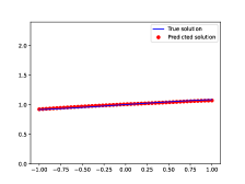
(a) SOC-MartNet:
$s\mapsto v(0,s\bm{e}_{1})$

(b) SOC-MartNet:
$s\mapsto v(0,s\bm{e}_{2})$

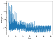
(c) SOC-MartNet:
Loss vs Epoch

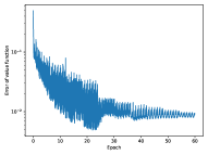
(d) SOC-MartNet:
RE vs Epoch

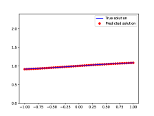
(e) FBSNN: $s\mapsto v(0,s\bm{e}_{1})$

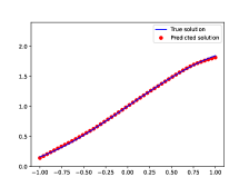
(f) FBSNN: $s\mapsto v(0,s\bm{e}_{2})$

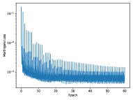
(g) FBSNN:
Loss vs Epoch

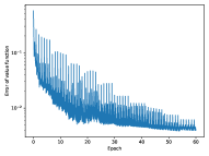
(h) FBSNN: RE vs Epoch

Figure 1: Numerical results for Problem (56) with $d=10$.

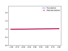
(a) SOC-MartNet:
$s\mapsto v(0,s\bm{e}_{1})$

(b) SOC-MartNet:
$s\mapsto v(0,s\bm{e}_{2})$

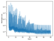
(c) SOC-MartNet:
Loss vs Epoch

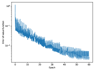
(d) SOC-MartNet:
RE vs Epoch

(e) FBSNN: $s\mapsto v(0,s\bm{e}_{1})$

(f) FBSNN: $s\mapsto v(0,s\bm{e}_{2})$

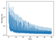
(g) FBSNN:
Loss vs Epoch

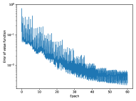
(h) FBSNN: RE vs Epoch

Figure 2: Numerical results for Problem (56) with $d=50$.

(a) SOC-MartNet:
$s\mapsto v(0,s\bm{e}_{1})$

(b) SOC-MartNet:
$s\mapsto v(0,s\bm{e}_{2})$

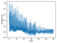
(c) SOC-MartNet:
Loss vs Epoch

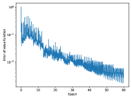
(d) SOC-MartNet:
RE vs Epoch

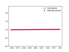
(e) FBSNN: $s\mapsto v(0,s\bm{e}_{1})$

(f) FBSNN: $s\mapsto v(0,s\bm{e}_{2})$

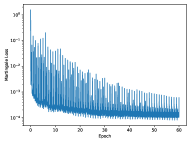
(g) FBSNN:
Loss vs Epoch

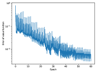
(h) FBSNN: RE vs Epoch

Figure 3: Numerical results for Problem (56) with $d=80$.

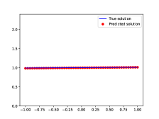
(a) SOC-MartNet:
$s\mapsto v(0,s\bm{e}_{1})$

(b) SOC-MartNet:
$s\mapsto v(0,s\bm{e}_{2})$

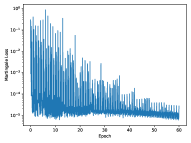
(c) SOC-MartNet:
Loss vs Epoch

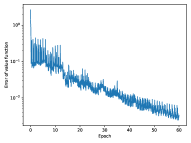
(d) SOC-MartNet:
RE vs Epoch

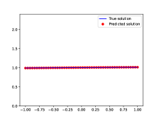
(e) FBSNN: $s\mapsto v(0,s\bm{e}_{1})$

(f) FBSNN: $s\mapsto v(0,s\bm{e}_{2})$

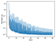
(g) FBSNN:
Loss vs Epoch

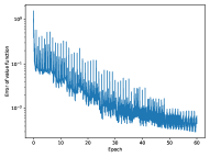
(h) FBSNN: RE vs Epoch

Figure 4: Numerical results for Problem (56) with $d=100$.

(a) $d=10$

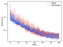
(b) $d=20$

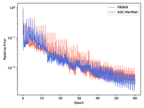
(c) $d=50$

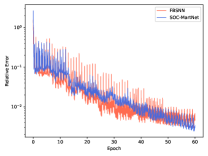
(d) $d=100$

Figure 5: The RE vs Epoch for SOC-MartNet and FBSNN in solving Problem (56).

4.2 Semilinear parabolic equation

We consider the following parabolic equation from [14, Section 4.3]:

$$\left\{\begin{aligned} &\left(\partial_{t}+\Delta_{x}\right)v(t,x)-\left|\partial_{x}v(t,x)\right|^{2}=0,\quad(t,x)\in[0,T)\times\mathbb{R}^{d},\\ &v(T,x)=1+g(x),\quad x\in\mathbb{R}^{d},\end{aligned}\right.$$ (58)

where $g(x):=\ln\left(\frac{1}{2}(1+\left|x\right|^{2})\right)$. Its analytic solution is that

$$v(t,x)=1-\ln\left(\mathbb{E}\left[\exp\left(-g(x+\sqrt{2}W_{T-t})\right)\right]\right),\quad(t,x)\in[0,T]\times\mathbb{R}^{d}.$$ (59)

To compute the absolute error of numerical solutions, the analytic solution in (59) is approximated by the Monte-Carlo method applied on the expectation using $10^{6}$ i.i.d. samples of $W_{T-t}$.

In the following, we present the numerical results of SOC-MarNet (Algorithm 2) and FBSNN for solving the parabolic problem (58).

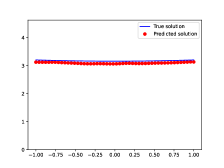
(a) SOC-MartNet:
$s\mapsto v(0,s\bm{e}_{1})$

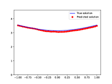
(b) SOC-MartNet:
$s\mapsto v(0,s\bm{e}_{2})$

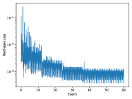
(c) SOC-MartNet:
Loss vs Epoch

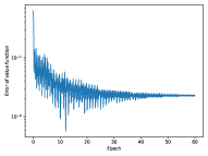
(d) SOC-MartNet:
RE vs Epoch

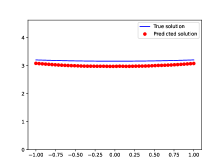
(e) FBSNN: $s\mapsto v(0,s\bm{e}_{1})$

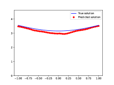
(f) FBSNN: $s\mapsto v(0,s\bm{e}_{2})$

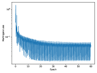
(g) FBSNN:
Loss vs Epoch

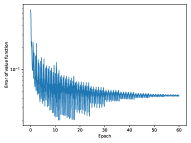
(h) FBSNN: RE vs Epoch

Figure 6: Numerical results for Problem (58) with $d=10$.

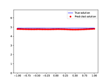
(a) SOC-MartNet:
$s\mapsto v(0,s\bm{e}_{1})$

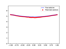
(b) SOC-MartNet:
$s\mapsto v(0,s\bm{e}_{2})$

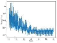
(c) SOC-MartNet:
Loss vs Epoch

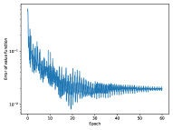
(d) SOC-MartNet:
RE vs Epoch

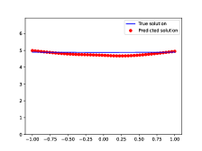
(e) FBSNN: $s\mapsto v(0,s\bm{e}_{1})$

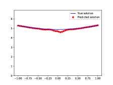
(f) FBSNN: $s\mapsto v(0,s\bm{e}_{2})$

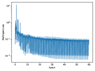
(g) FBSNN:
Loss vs Epoch

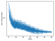
(h) FBSNN: RE vs Epoch

Figure 7: Numerical results for Problem (58) with $d=50$.

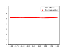
(a) SOC-MartNet:
$s\mapsto v(0,s\bm{e}_{1})$

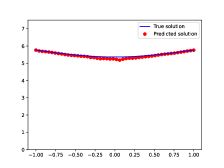
(b) SOC-MartNet:
$s\mapsto v(0,s\bm{e}_{2})$

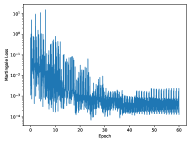
(c) SOC-MartNet:
Loss vs Epoch

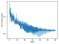
(d) SOC-MartNet:
RE vs Epoch

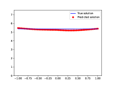
(e) FBSNN: $s\mapsto v(0,s\bm{e}_{1})$

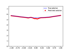
(f) FBSNN: $s\mapsto v(0,s\bm{e}_{2})$

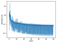
(g) FBSNN:
Loss vs Epoch

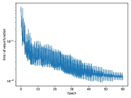
(h) FBSNN: RE vs Epoch

Figure 8: Numerical results for Problem (58) with $d=80$.

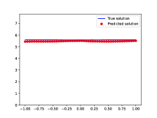
(a) SOC-MartNet:
$s\mapsto v(0,s\bm{e}_{1})$

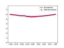
(b) SOC-MartNet:
$s\mapsto v(0,s\bm{e}_{2})$

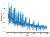
(c) SOC-MartNet:
Loss vs Epoch

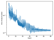
(d) SOC-MartNet:
RE vs Epoch

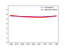
(e) FBSNN: $s\mapsto v(0,s\bm{e}_{1})$

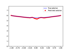
(f) FBSNN: $s\mapsto v(0,s\bm{e}_{2})$

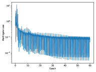
(g) FBSNN:
Loss vs Epoch

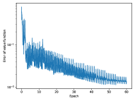
(h) FBSNN: RE vs Epoch

Figure 9: Numerical results for Problem (58) with $d=100$.

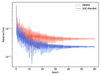
(a) $d=10$

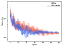
(b) $d=20$

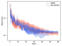
(c) $d=50$

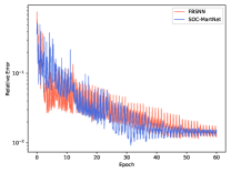
(d) $d=100$

Figure 10: The RE vs Epoch for SOC-MartNet and FBSNN in solving Problem (58).

4.3 Non-degenerated HJB equation without using explicit form of $\inf_{u}H$

We consider the following HJB equation from [1, Section 3.1]:

$$\left\{\begin{aligned} &\left(\partial_{t}+\Delta_{x}\right)v(t,x)+\inf_{\kappa\in\mathbb{R}^{d}}\left(2\kappa^{\top}\partial_{x}v(t,x)+\left|\kappa\right|^{2}\right)=0,\quad(t,x)\in[0,T)\times\mathbb{R}^{d},\\ &v(T,x)=1+g(x),\quad x\in\mathbb{R}^{d},\end{aligned}\right.$$ (60)

where $g(x):=\ln\left(\frac{1}{2}(1+\left|x\right|^{2})\right)$. The analytic solution of (60) is identical to (59). The HJB equation (60) is associated with the SOCP:

$$u^{*}=\mathop{\arg\min}_{u\in\mathcal{U}_{\mathrm{ad}}}J(u),\quad J(u):=1+\mathbb{E}\left[\int_{0}^{T}\left|u_{s}\right|^{2}\,\mathrm{d}s+g\left(X_{T}^{u}\right)\right],$$ (61)

$$\mathcal{U}_{\mathrm{ad}}=\left\{u:[0,T]\times\Omega\to\mathbb{R}^{d}:\text{$u$ is $\mathbb{F}^{B}$-adapted}\right\},$$ (62)

$$X_{t}^{u}=X_{0}+\int_{0}^{t}2u_{s}\,\mathrm{d}s+\int_{0}^{t}\sqrt{2}\,\mathrm{d}B_{s},\quad t\in[0,T],$$ (63)

where $B$ is a $d$-dimensional standard Brownian motion. The optimal feedback control is that

$$u^{*}(t,x)=-\partial_{x}v(t,x),\quad(t,x)\in[0,T]\times\mathbb{R}^{d}.$$

In the following, we present the numerical results of SOC-MarNet (Algorithm 1) for the HJB equation (60), where no explicit form is used for $\inf_{\kappa\in U}H$, and and approximated by $u_{\alpha}$.

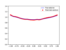
(a) SOC-MartNet:
$s\mapsto v(0,s\bm{e}_{1})$

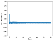
(b) SOC-MartNet:
Hamiltonian vs Epoch

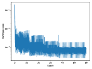
(c) SOC-MartNet:
Mart. Loss vs Epoch

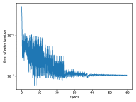
(d) SOC-MartNet:
RE of $v$ vs Epoch

Figure 11: Numerical results for the HJB equation (60) with $d=1$. The running time of SOC-MartNet is 91 seconds for $60$ epoch.

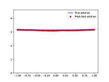
(a) SOC-MartNet:
$s\mapsto v(0,s\bm{e}_{1})$

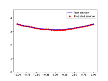
(b) SOC-MartNet:
$s\mapsto v(0,s\bm{e}_{2})$

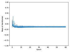
(c) SOC-MartNet:
Hamiltonian vs Epoch

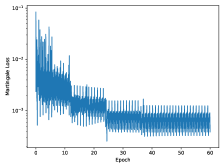
(d) SOC-MartNet:
Mart. Loss vs Epoch

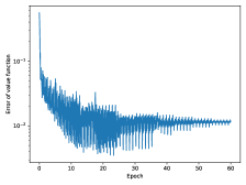
(e) SOC-MartNet:
RE of $v$ vs Epoch

Figure 12: Numerical results for the HJB equation (60) with $d=10$. The running time of SOC-MartNet is 92 seconds for $60$ epoch.

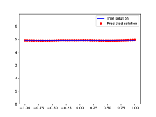
(a) SOC-MartNet:
$s\mapsto v(0,s\bm{e}_{1})$

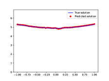
(b) SOC-MartNet:
$s\mapsto v(0,s\bm{e}_{2})$

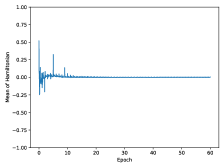
(c) SOC-MartNet:
Hamiltonian vs Epoch

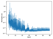
(d) SOC-MartNet:
Mart. Loss vs Epoch

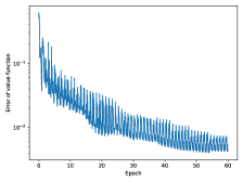
(e) SOC-MartNet:
RE of $v$ vs Epoch

Figure 13: Numerical results for the HJB equation (60) with $d=50$. The running time of SOC-MartNet is 162 seconds for $60$ epoch.

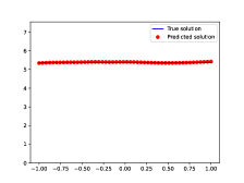
(a) SOC-MartNet:
$s\mapsto v(0,s\bm{e}_{1})$

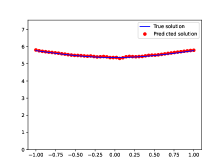
(b) SOC-MartNet:
$s\mapsto v(0,s\bm{e}_{2})$

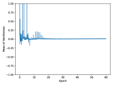
(c) SOC-MartNet:
Hamiltonian vs Epoch

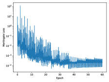
(d) SOC-MartNet:
Mart. Loss vs Epoch

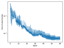
(e) SOC-MartNet:
RE of $v$ vs Epoch

Figure 14: Numerical results for the HJB equation (60) with $d=80$. The running time of SOC-MartNet is 295 seconds for $60$ epoch.

(a) SOC-MartNet:
$s\mapsto v(0,s\bm{e}_{1})$

(b) SOC-MartNet:
$s\mapsto v(0,s\bm{e}_{2})$

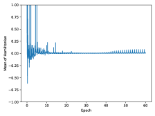
(c) SOC-MartNet:
Hamiltonian vs Epoch

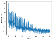
(d) SOC-MartNet:
Mart. Loss vs Epoch

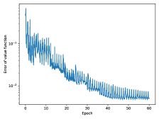
(e) SOC-MartNet:
RE of $v$ vs Epoch

Figure 15: Numerical results for the HJB equation (60) with $d=100$. The running time of SOC-MartNet is 438 seconds for $60$ epoch.

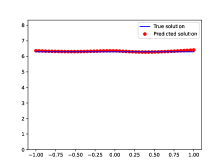
(a) SOC-MartNet:
$s\mapsto v(0,s\bm{e}_{1})$

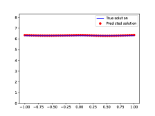
(b) SOC-MartNet:
$s\mapsto v(0,s\bm{e}_{2}/\left|\bm{e}_{2}\right|)$

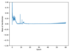
(c) SOC-MartNet:
Hamiltonian vs Epoch

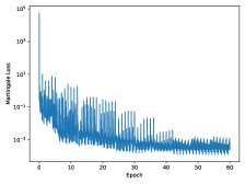
(d) SOC-MartNet:
Mart. Loss vs Epoch

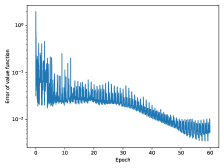
(e) SOC-MartNet:
RE of $v$ vs Epoch

Figure 16: Numerical results for the HJB equation (60) with $d=200$. The running time of SOC-MartNet is 1364 seconds for $60$ epoch.

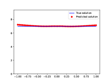
(a) SOC-MartNet:
$s\mapsto v(0,s\bm{e}_{1})$

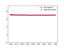
(b) SOC-MartNet:
$s\mapsto v(0,s\bm{e}_{2}/\left|\bm{e}_{2}\right|)$

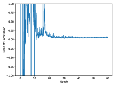
(c) SOC-MartNet:
Hamiltonian vs Epoch

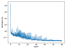
(d) SOC-MartNet:
Mart. Loss vs Epoch

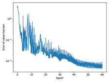
(e) SOC-MartNet:
RE of $v$ vs Epoch

Figure 17: Numerical results for the HJB equation (60) with $d=400$. The running time of SOC-MartNet is 4009 seconds for $60$ epoch.

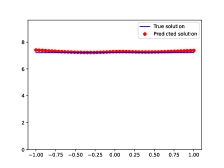
(a) SOC-MartNet:
$s\mapsto v(0,s\bm{e}_{1})$

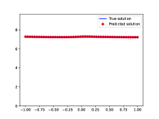
(b) SOC-MartNet:
$s\mapsto v(0,s\bm{e}_{2}/\left|\bm{e}_{2}\right|)$

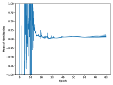
(c) SOC-MartNet:
Hamiltonian vs Epoch

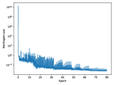
(d) SOC-MartNet:
Mart. Loss vs Epoch

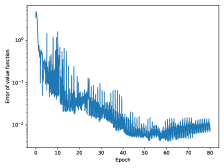
(e) SOC-MartNet:
RE of $v$ vs Epoch

Figure 18: Numerical results for the HJB equation (60) with $d=500$. The running time of SOC-MartNet is 8946 seconds for $80$ epoch.

5 Conclusions

In this paper, we propose a novel numerical method SOC-MartNet based on the DeepMartNet [8; 7] combined with adversarial learning. First, we introduce a Hamiltonian process and a cost process, both of which are represented by a control network and a value network. Then, the HJB equation is reformulated as an optimization problem, i.e., minimizing the Hamiltonian process with the cost process restricted to a martingale. The martingale property of the cost process is further enforced by adversarial learning, whose loss function is built upon the projection property of conditional expectations. Numerical results show that the proposed SOC-MartNet is effective and efficient for solving equations with dimension up to $500$, and especially to SCOPs when the $\inf H$ has no explicit expressions.

References

- [1] Achref Bachouch, Côme Huré, Nicolas Langrené, and Huyên Pham. Deep neural networks algorithms for stochastic control problems on finite horizon: numerical applications. Methodol. Comput. Appl. Probab., 24(1):143–178, 2022.
- [2] Guy Barles and Espen Robstad Jakobsen. On the convergence rate of approximation schemes for Hamilton-Jacobi-Bellman equations. M2AN Math. Model. Numer. Anal., 36(1):33–54, 2002.
- [3] R. W. Beard, G. N. Saridis, and J. T. Wen. Approximate solutions to the time-invariant Hamilton-Jacobi-Bellman equation. J. Optim. Theory Appl., 96(3):589–626, 1998.
- [4] Randal W. Beard, George N. Saridis, and John T. Wen. Galerkin approximations of the generalized Hamilton-Jacobi-Bellman equation. Automatica J. IFAC, 33(12):2159–2177, 1997.
- [5] Richard Bellman. Dynamic programming. Princeton University Press, Princeton, NJ, 1957.
- [6] Simone Cacace, Emiliano Cristiani, Maurizio Falcone, and Athena Picarelli. A patchy dynamic programming scheme for a class of Hamilton-Jacobi-Bellman equations. SIAM J. Sci. Comput., 34(5):A2625–A2649, 2012.
- [7] Wei Cai. DeepMartNet – a martingale based deep neural network learning algorithm for eigenvalue/BVP problems and optimal stochastic controls, 2023, arXiv:2307.11942 [math.NA].
- [8] Wei Cai, Andrew He, and Daniel Margolis. DeepMartNet – a martingale based deep neural network learning method for Dirichlet BVP and eigenvalue problems of elliptic pdes, 2023, arXiv:2311.09456 [math.NA].
- [9] Michael G. Crandall, Hitoshi Ishii, and Pierre-Louis Lions. User’s guide to viscosity solutions of second order partial differential equations. Bull. Amer. Math. Soc. (N.S.), 27(1):1–67, 1992.
- [10] Michael G. Crandall and Pierre-Louis Lions. Viscosity solutions of Hamilton-Jacobi equations. Trans. Amer. Math. Soc., 277(1):1–42, 1983.
- [11] Jérôme Darbon, Gabriel P. Langlois, and Tingwei Meng. Overcoming the curse of dimensionality for some Hamilton-Jacobi partial differential equations via neural network architectures. Res. Math. Sci., 7(3):Paper No. 20, 50, 2020.
- [12] Jérôme Darbon and Tingwei Meng. On some neural network architectures that can represent viscosity solutions of certain high dimensional Hamilton-Jacobi partial differential equations. J. Comput. Phys., 425:Paper No. 109907, 16, 2021.
- [13] Sergey Dolgov, Dante Kalise, and Karl K. Kunisch. Tensor decomposition methods for high-dimensional Hamilton-Jacobi-Bellman equations. SIAM J. Sci. Comput., 43(3):A1625–A1650, 2021.
- [14] Weinan E, Jiequn Han, and Arnulf Jentzen. Deep learning-based numerical methods for high-dimensional parabolic partial differential equations and backward stochastic differential equations. Commun. Math. Stat., 5(4):349–380, 2017.
- [15] Weinan E, Jiequn Han, and Arnulf Jentzen. Algorithms for solving high dimensional PDEs: from nonlinear Monte Carlo to machine learning. Nonlinearity, 35(1):278–310, 2022.
- [16] Wendell H. Fleming and Raymond W. Rishel. Deterministic and stochastic optimal control, volume No. 1 of Applications of Mathematics. Springer-Verlag, Berlin-New York, 1975.
- [17] Yu Fu, Weidong Zhao, and Tao Zhou. Highly accurate numerical schemes for stochastic optimal control via FBSDEs. Numer. Math. Theory Methods Appl., 13(2):296–319, 2020.
- [18] Jean-François Le Gall. Brownian Motion, Martingales, and Stochastic Calculus. Springer Cham, 2016.
- [19] Zhiwei Gao, Liang Yan, and Tao Zhou. Failure-informed adaptive sampling for PINNs. SIAM J. Sci. Comput., 45(4):A1971–A1994, 2023.
- [20] Bo Gong, Wenbin Liu, Tao Tang, Weidong Zhao, and Tao Zhou. An efficient gradient projection method for stochastic optimal control problems. SIAM J. Numer. Anal., 55(6):2982–3005, 2017.
- [21] Ling Guo, Hao Wu, Xiaochen Yu, and Tao Zhou. Monte Carlo fPINNs: deep learning method for forward and inverse problems involving high dimensional fractional partial differential equations. Comput. Methods Appl. Mech. Engrg., 400:Paper No. 115523, 17, 2022.
- [22] Jiequn Han and Weinan E. Deep learning approximation for stochastic control problems. Deep Reinforcement Learning Workshop, NIPS, 2016, arXiv:1611.07422 [cs.LG].
- [23] Côme Huré, Huyên Pham, Achref Bachouch, and Nicolas Langrené. Deep neural networks algorithms for stochastic control problems on finite horizon: convergence analysis. SIAM J. Numer. Anal., 59(1):525–557, 2021.
- [24] Côme Huré, Huyên Pham, and Xavier Warin. Deep backward schemes for high-dimensional nonlinear PDEs. Math. Comp., 89(324):1547–1579, 2020.
- [25] Hitoshi Ishii. On uniqueness and existence of viscosity solutions of fully nonlinear second-order elliptic PDEs. Comm. Pure Appl. Math., 42(1):15–45, 1989.
- [26] Robert Jensen. The maximum principle for viscosity solutions of fully nonlinear second order partial differential equations. Arch. Rational Mech. Anal., 101(1):1–27, 1988.
- [27] Shaolin Ji, Shige Peng, Ying Peng, and Xichuan Zhang. Solving stochastic optimal control problem via stochastic maximum principle with deep learning method. J. Sci. Comput., 93(1):Paper No. 30, 28, 2022.
- [28] Dante Kalise and Karl Kunisch. Polynomial approximation of high-dimensional Hamilton-Jacobi-Bellman equations and applications to feedback control of semilinear parabolic PDEs. SIAM J. Sci. Comput., 40(2):A629–A652, 2018.
- [29] Wei Kang and Lucas C. Wilcox. Mitigating the curse of dimensionality: sparse grid characteristics method for optimal feedback control and HJB equations. Comput. Optim. Appl., 68(2):289–315, 2017.
- [30] Idris Kharroubi, Nicolas Langrené, and Huyên Pham. A numerical algorithm for fully nonlinear HJB equations: an approach by control randomization. Monte Carlo Methods Appl., 20(2):145–165, 2014.
- [31] Idris Kharroubi, Nicolas Langrené, and Huyên Pham. Discrete time approximation of fully nonlinear HJB equations via BSDEs with nonpositive jumps. Ann. Appl. Probab., 25(4):2301–2338, 2015.
- [32] Idris Kharroubi and Huyên Pham. Feynman-Kac representation for Hamilton-Jacobi-Bellman IPDE. Ann. Probab., 43(4):1823–1865, 2015.
- [33] Achim Klenke. Probability Theory. Springer Cham, third edition, 2020.
- [34] N. V. Krylov. Controlled diffusion processes, volume 14 of Applications of Mathematics. Springer-Verlag, New York-Berlin, 1980. Translated from the Russian by A. B. Aries.
- [35] N. V. Krylov. Nonlinear elliptic and parabolic equations of the second order, volume 7 of Mathematics and its Applications (Soviet Series). D. Reidel Publishing Co., Dordrecht, 1987. Translated from the Russian by P. L. Buzytsky [P. L. Buzytskiĭ].
- [36] K. Kunisch, S. Volkwein, and L. Xie. HJB-POD-based feedback design for the optimal control of evolution problems. SIAM J. Appl. Dyn. Syst., 3(4):701–722, 2004.
- [37] Pierre-Louis Lions. Generalized solutions of Hamilton-Jacobi equations, volume 69 of Research Notes in Mathematics. Pitman (Advanced Publishing Program), Boston, Mass.-London, 1982.
- [38] Tenavi Nakamura-Zimmerer, Qi Gong, and Wei Kang. Adaptive deep learning for high-dimensional Hamilton-Jacobi-Bellman equations. SIAM J. Sci. Comput., 43(2):A1221–A1247, 2021.
- [39] Carmeliza Navasca and Arthur J. Krener. Patchy solutions of Hamilton-Jacobi-Bellman partial differential equations. In Modeling, estimation and control, volume 364 of Lect. Notes Control Inf. Sci., pages 251–270. Springer, Berlin, 2007.
- [40] Bernt Ø ksendal. Stochastic differential equations. Universitext. Springer-Verlag, Berlin, sixth edition, 2003. An introduction with applications.
- [41] S Osher and CW Shu. High-order essentially nonoscillatory schemes for hamilton–jacobi equations. SIAM Journal on numerical analysis, 4:907–922, 1991.
- [42] Huyên Pham. Continuous-time stochastic control and optimization with financial applications, volume 61 of Stochastic Modelling and Applied Probability. Springer-Verlag, Berlin, 2009.
- [43] M. Raissi, P. Perdikaris, and G. E. Karniadakis. Physics-informed neural networks: a deep learning framework for solving forward and inverse problems involving nonlinear partial differential equations. J. Comput. Phys., 378:686–707, 2019.
- [44] S. Richardson and S. Wang. Numerical solution of Hamilton-Jacobi-Bellman equations by an exponentially fitted finite volume method. Optimization, 55(1-2):121–140, 2006.
- [45] Iain Smears and Endre Süli. Discontinuous Galerkin finite element approximation of Hamilton-Jacobi-Bellman equations with Cordes coefficients. SIAM J. Numer. Anal., 52(2):993–1016, 2014.
- [46] S. Wang, L. S. Jennings, and K. L. Teo. Numerical solution of Hamilton-Jacobi-Bellman equations by an upwind finite volume method. volume 27, pages 177–192. 2003. International Workshop on Optimization with High-Technology Applications (OHTA 2000) (Hong Kong).
- [47] Jiongmin Yong and Xun Yu Zhou. Stochastic controls, volume 43 of Applications of Mathematics (New York). Springer-Verlag, New York, 1999. Hamiltonian systems and HJB equations.
- [48] Yaohua Zang, Gang Bao, Xiaojing Ye, and Haomin Zhou. Weak adversarial networks for high-dimensional partial differential equations. J. Comput. Phys., 411:109409, 14, 2020.
- [49] Wenzhong Zhang and Wei Cai. FBSDE based neural network algorithms for high-dimensional quasilinear parabolic PDEs. J. Comput. Phys., 470:Paper No. 111557, 14, 2022.
- [50] Weidong Zhao, Tao Zhou, and Tao Kong. High order numerical schemes for second-order FBSDEs with applications to stochastic optimal control. Commun. Comput. Phys., 21(3):808–834, 2017.
- [51] Mo Zhou, Jiequn Han, and Jianfeng Lu. Actor-critic method for high dimensional static Hamilton-Jacobi-Bellman partial differential equations based on neural networks. SIAM J. Sci. Comput., 43(6):A4043–A4066, 2021.