The Loewner framework for parametric systems: Taming the curse of dimensionality

Abstract

The Loewner framework is an interpolatory framework for the approximation of linear and nonlinear systems. The purpose here is to extend this framework to linear parametric systems with an arbitrary number $\ord$ of parameters. One main innovation established here is the construction of data-based realizations for any number of parameters. Equally importantly, we show how to alleviate the computational burden, by avoiding the explicit construction of large-scale $\ord$-dimensional Loewner matrices of size $N\times N$. This reduces the complexity from ${\cal O}(N^{3})$ to about ${\cal O}(N^{1.4})$, thus taming the curse of dimensionality and making the solution scalable to very large data sets. To achieve this, a new generalized multivariate rational function realization is defined. Then, we introduce the $\ord$-dimensional multivariate Loewner matrices and show that they can be computed by solving a coupled set of Sylvester equations. The null space of these Loewner matrices then allows the construction of the multivariate barycentric transfer function. The principal result of this work is to show how the null space of the $\ord$-dimensional Loewner matrix can be computed using a sequence of 1-dimensional Loewner matrices, leading to a drastic computational burden reduction. Finally, we suggest two algorithms (one direct and one iterative) to construct, directly from data, multivariate (or parametric) realizations ensuring (approximate) interpolation. Numerical examples highlight the effectiveness and scalability of the method.

First, we propose a generalized realization form for rational functions in $\ord$-variables (for any $\ord$), which are described in the Lagrange basis. Secondly, we show that the corresponding $\ord$-dimensional Loewner matrix is the solution of a cascaded Sylvester equation set. Finally, we demonstrate that the barycentric coefficients can be obtained using a sequence of 1-dimensional Loewner matrices instead of the large-scale $\ord$-dimensional one, drastically reducing the computational effort.

1 Introduction

The context, motivation, and problem statement are first presented. Since it is the principal mathematical tool of the developed method, a brief historical review of Loewner matrix-driven methods is given. Then, the contributions and paper overview are listed.

1.1 Motivation and context: the non-intrusive data-driven model construction

Multivariate rational model interpolation addresses the problem of constructing a reduced order model that well captures the behavior of a potentially large-scale model depending on multiple variables. In the context of dynamical systems governed by differential and algebraic equations, the multivariate nature mainly comes from the parametric dependency of the underlying system or model. These parameters account for physical characteristics such as mass, length, or material property (in mechanical systems), flow velocity, temperature (in fluid cases), chemical properties (in biological systems), etc. In engineering applications, the parameters are embedded within the model as tuning variables for the output of interest. The challenges and motivations for dynamical multivariate/parametric reduced order model (pROM) construction stem from three inevitable facts about modern computing and actual engineers’ concerns:

• First, accurate modeling often leads to large-scale dynamical systems with complex dynamics, for which simulation times and data storage needs become prohibitive, or at least impractical for engineers and practitioners;

• Second, the explicit mathematical model describing the underlying phenomena may not be always accessible while input-output data may be measured either from a computer-based (black-box) simulator or directly from a physical experiment; as a consequence, the internal variables of the dynamical phenomena are usually too large to be stored or simply inaccessible;

• Third, a potentially large number of parameters may be necessary, to be used in the next steps of the process.

Often, complex and accurate parametric models are needed by practitioners to perform simulations, forecasting, parametric uncertainty propagation, and optimization in a broad sense. The goals could be to better understand and analyze the physics, to tune coefficients, to optimize the system, or to construct parameterized control laws. As these objectives often require a multi-query model-based optimization process, the complexity dictates the accuracy, scalability, and applicability of the approach, it is relevant to seek a pROM with low complexity.

1.2 Literature overview

In the last decade, there has been a lot of effort invested into devising reliable and accurate model reduction (intrusive) and reduced-order modeling (non-intrusive) methods, synthesized in a multitude of methodologies continuously developed in the last years [3, 10, 32, 5, 12, 13]. For the class of parametric systems, the comprehensive review contribution in [14] provides an exhaustive account of projection-based methods, from the 2000s until the middle of 2010s.

Additionally, relatively new approaches use time-domain snapshot data to compute reduced-order models, such as operator inference (OpInf) [46] and dynamic mode decomposition (DMD) [50]. Extension of such methods to parameterized dynamical systems have been recently proposed, for OpInf in [57, 40] and also for DMD in [2, 49].

For the class of frequency-domain methods, we mainly concentrate in what follows on interpolation-based methods. For other classes of projection-based methods we refer the reader to the survey [14]. As explained in this review paper, reduced-order models for parametric systems are typically computed by means of projection, using either a local or a global basis for matrix or transfer function interpolation. Here, we mention some of the relevant contributions in the last years [1, 23, 58, 25]. Additionally, optimal and quasi-optimal approaches have also been proposed in [9, 33, 41], which try to impose optimality in certain norms, e.g., in the $\mathcal{H}_{2}\otimes\mathcal{L}_{2}$ norm. Finally, implementation issues for pMOR with software packages in Python programming language were addressed in [42].

Non-intrusive methods based on interpolating or approximately matching (using least squares fitting) of transfer function measurements (of the underlying parameterized rational transfer function) have been quite prolific in the last decades, with the following prominent contributions mentioned below:

• Extensions of the Loewner Framework (LF) to multivariate rational approximation by interpolation: [6, 34, 54] together with the AAA algorithm (Adaptive Antoulas-Anderson) for multivariate functions [48, 24], and an extension of LF with orthogonal polynomials [56].

• Extensions of the Vector Fitting framework to multivariate rational approximation, including the generalized Sanathanan-Koerner iteration in [16, 59]; these works are mostly concerned with imposing stability and passivity guarantees for macro model generation in the field of electronics.

We also mention other related works, such as [19, 8, 45, 18]. Recent trends in harnessing the power of artificial neural networks (ANNs) in connection to deep learning have allowed increased computational power and increased the usability of the methods. Established methods involve incorporating PINNs or DeepONets in the solution or analysis of parametric PDEs, such as in [11, 21, 29].

1.3 Connection to other fields

Tensors represent generalizations of vectors and matrices in multiple dimensions, possessing at least one extra dimension (a minimum of three). Applications include, among others, some from the fields of signal processing (e.g., array processing), scientific computing (e.g., discretization of multivariate functions), and more recently, quantum computing (e.g., simulation of quantum many-body). We refer the reader to [36] for additional information and detailed discussion on the matter. However, explicitly working with tensors, especially of higher dimensions, is not a trivial task. The number of elements in a tensor increases exponentially with the number of dimensions, and so do the computational/memory requirements. The exponential dependency together with the challenges that arise from it, are connected to the curse of dimensionality (C-o-D).

Tensor decompositions are particularly important and relevant for several strenuous computational tasks since they can potentially alleviate the curse of dimensionality that occurs when working with high-dimensional tensors, as explained in [53]. Such a decomposition can accurately represent and substitute the tensor, i.e., one may use it instead of explicitly using the original tensor itself. More details and an extensive literature survey of low-rank tensor approximation techniques, including canonical polyadic decomposition, Tucker decomposition, low multilinear rank approximation, and tensor trains and networks can be found in [27].

Tensorization and Loewner matrices were recently connected in the contribution [20]. There, a collection of one-dimensional (standard) Loewner matrices is reshaped as a third-dimensional tensor (named ”Loewnerization”), for which the block term decomposition (BTD) is applied. The application of interest is blind signal separation. This approach was recently extended in [52], to the MIMO case.

Nonlinear eigenvalue problems (NEPs) represent an established field of study. A NEP can be viewed as a generalization of the (ordinary) eigenvalue problem to equations that depend nonlinearly on the eigenvalue. Linearization techniques allow reformulating any polynomial EP as a larger linear eigenvalue problem and then applying the established (classical) algorithms to solve it. Other linearizations have been proposed involving rational approximation [31], and [37, 30], which involve the usage of the rational Krylov or the AAA algorithms, together with [17] which uses the Loewner and Hankel frameworks in the context of contour integrals.

1.4 Problem statement

A linear-in-state dynamical system parameterized in terms of parameters included in the set ${\cal S}=[\mathstrut^{2}s,\dots,\mathstrut^{\ord}s]^{\top}\subset{\mathbb{C}}^{\ord-1}$, is characterized in state-space representation by the following equations:

$${\mathbf{E}}({\cal S})\dot{{\mathbf{x}}}(t;{\cal S})={\mathbf{A}}({\cal S}){\mathbf{x}}(t;{\cal S})+{\mathbf{B}}({\cal S}){\mathbf{u}}(t),~{}~{}{\mathbf{y}}(t;{\cal S})={\mathbf{C}}({\cal S}){\mathbf{x}}(t;{\cal S}),$$ (1)

where $\dot{{\mathbf{x}}}(t;{\cal S})$ refers to the derivative of ${\mathbf{x}}(t;{\cal S})\in{\mathbb{R}}^{M}$, with respect to the time variable $t$. Additionally, the $n_{u}$ control inputs are collected in the vector ${\mathbf{u}}(t)\in{\mathbb{R}}^{n_{u}}$, while the $n_{y}$ outputs are observed in the vector ${\mathbf{y}}(t;{\cal S})\in{\mathbb{R}}^{n_{y}}$. Finally, the dimensions of the system matrices appearing in the state-space realization eq. 1 are as follows: ${\mathbf{E}}({\cal S}),{\mathbf{A}}({\cal S})\in{\mathbb{R}}^{M\times M}$, ${\mathbf{B}}({\cal S})\in{\mathbb{R}}^{M\times n_{u}}$, ${\mathbf{C}}({\cal S})\in{\mathbb{R}}^{n_{y}\times M}$. For simplicity of exposition, we consider only the single-input and single-output (SISO) scenario in what follows, i.e., $n_{u}=n_{y}=1$. Although extension to multi-input multi-output (MIMO) systems is relevant, it will be the topic of future research, e.g. following the formulation exposed in [54]. In the sequel, particular attention is allocated to the exposition of a solution that tames the curse of dimensionality (C-o-D).

Remark 1.1 (Focus on the SISO case).

To simplify the exposition, we consider solely the case of single-input and single-output (SISO) systems (i.e. $n_{u}=n_{y}=1$). Although extension to multi-input multi-output (MIMO) systems is relevant, it will be the topic of future research, e.g. following the formulation exposed in [54]. In the sequel, particular attention is allocated to the exposition of a solution that tames the curse of dimensionality ( C-o-D) which is a more challenging and fundamental problem.

Transforming the differential equation in eq. 1 using the unilateral Laplace transform, the time variable $t$ becomes $\mathstrut{}^{1}s$, and solving for the transformed state variable, we have: ${\mathbf{X}}(\mathstrut^{1}s;{\cal S})=\left[\mathstrut{}^{1}s{\mathbf{E}}({\cal S})-{\mathbf{A}}({\cal S})\right]^{-1}{\mathbf{B}}({\cal S}){\mathbf{U}}(\mathstrut^{1}s)$. Similarly, transforming the second equation in eq. 1 we obtain: ${\mathbf{Y}}(\mathstrut^{1}s;{\cal S})={\mathbf{C}}({\cal S}){\mathbf{X}}(\mathstrut^{1}s;{\cal S})$. These equations yield to ${\mathbf{Y}}(\mathstrut^{1}s;{\cal S})={\mathbf{C}}({\cal S})\left[\mathstrut{}^{1}s{\mathbf{E}}({\cal S})-{\mathbf{A}}({\cal S})\right]^{-1}{\mathbf{B}}({\cal S}){\mathbf{U}}(\mathstrut^{1}s)$. The transfer function of the parametric linear time-invariant (pLTI) system in eq. 1 is a multivariate rational transfer function, given by

$${\mathbf{H}}(\mathstrut^{1}s,\mathstrut^{2}s,\dots,\mathstrut^{\ord}s)={\mathbf{C}}({\cal S})\left[\mathstrut{}^{1}s{\mathbf{E}}({\cal S})-{\mathbf{A}}({\cal S})\right]^{-1}{\mathbf{B}}({\cal S})\in{\mathbb{C}}.$$ (2)

It involves $\ord$ variables $\mathstrut{}^{j}s\in{\mathbb{C}}$, $j=1,\dots,\ord$, including the ones in the set ${\cal S}$ but also the frequency or Laplace variable, which is denoted by $\mathstrut{}^{1}s$.

We denote the complexity of each variable $\mathstrut{}^{j}s$ with the value $d_{j}$ (the highest degree in which the variable occurs in both polynomials describing the rational function shown above) and say that ${\mathbf{H}}(\mathstrut^{1}s,\mathstrut^{2}s,\dots,\mathstrut^{\ord}s)$ in eq. 2 is of complexity $(d_{1},d_{2},\dots,d_{\ord})$.

As we are interested in the non-intrusive data-driven setup, let us now consider that the function in eq. 2 is not explicitly known. Instead, one has access to evaluations at (support or interpolatory) points $\mathstrut{}^{1}\lambda_{j_{1}},\mathstrut^{2}\lambda_{j_{2}},\dots,\mathstrut^{\ord}\lambda_{j_{\ord}}$ along $\mathstrut{}^{1}s,\mathstrut^{2}s,\dots\mathstrut^{\ord}s$, leading to measurements ${\mathbf{w}}_{j_{1},j_{2},\dots,j_{\ord}}$, for $j_{1},j_{2},\dots,j_{\ord}=1,\ldots,k_{1},k_{2},\dots,k_{\ord}$. Under some assumptions detailed in the sequel, we seek a reduced multivariate rational model, pROM, $\hat{\mathbf{H}}$ given as

$$\hat{\mathbf{H}}(\mathstrut^{1}s,\mathstrut^{2}s,\dots,\mathstrut^{\ord}s)={\mathbf{G}}\boldsymbol{\Phi}(\mathstrut^{1}s,\mathstrut^{2}s,\dots,\mathstrut^{\ord}s)^{-1}{\mathbf{W}}\in{\mathbb{C}},$$ (3)

where the vectors ${\mathbf{G}}^{\top},{\mathbf{W}}\in{\mathbb{C}}^{m}$ and square matrix $\boldsymbol{\Phi}\in{\mathbb{C}}^{m\times m}$ define a generalized realization, detailed latter. We denote this realization with the triple $({\mathbf{G}},\boldsymbol{\Phi},{\mathbf{W}})$, being the output, inverse of the resolvent, and input operators.

In the sequel, we concentrate on continuous-time dynamical systems. Therefore, the first variable $\mathstrut{}^{1}s$ will be associated with the dynamic Laplace (frequency) variable, while $\mathstrut{}^{2}s,\dots,\mathstrut^{\ord}s$ will stand as non-dynamic parametric variables (typically, they are real-valued but a complex form is also possible). Note that a similar discrete sampled-time model can be obtained using the $z$-transform (see e.g. [55]).

1.5 Historical notes

The Loewner matrix was introduced by Karl Löwner in the seminal paper published nine decades ago [38]. It has been further studied and used in multiple works dealing with data-driven rational function approximation with application in system theory at large. In [4], the Loewner matrix constructed from data is used to compute the barycentric coefficients to obtain the rational approximating function in the Lagrange basis. This is also known as the one-sided Loewner framework. One major update was proposed in 2007 by [39], introducing the two-sided Loewner framework, allowing the construction of a rational model with minimal McMillan degree and embedding a realization with minimal order, directly from the data. Then, [7] provides a comprehensive review of the case of single-variable linear systems, gathering most of the results up to 2017. Later in [6] the one-sided framework is extended to two variables/parameters, and its corresponding Lagrangian realization is derived. Later in [34], the multi-parameter Loewner framework (mpLF) is presented together (for up to three parameters) with the barycentric form, but without the description of a realization. Recently, handbook and tutorial contributions for LF, with its extensions and many applications, were proposed in [7, 35]. Finally, [26] provides a comprehensive overview including parametric and nonlinear Loewner extensions, and practical applications and test cases from aerospace engineering and computational fluid dynamics.

The AAA algorithm in [43] represents an iterative and adaptive version of the method in [4], that makes use of the barycentric representation of rational interpolants. For more details on barycentric forms, and connections to Lagrange interpolation, we refer the reader to [15]. In [48], the parametric AAA (p-AAA) algorithm is introduced. This extends the original AAA formulation of [43] to multivariate problems appearing in the modeling of parametric dynamical systems. The p-AAA can be viewed as an adaptation of the mpLF, in that it also uses multi-dimensional Loewner matrices and computes barycentric forms of the fitted rational functions. The p-AAA algorithm chooses the interpolation points in a greedy manner and enriches the Lagrange bases until an approximation quality is enforced on the available data. Then, extensions of the AAA algorithm to linear systems with quadratic outputs (characterized by transfer functions in one and in two variables) were proposed in [25]. For more extensions and applications of the AAA algorithm, we refer the reader to [44].

In addition, multiple application-oriented research papers utilizing the Loewner framework have been suggested, as well as multiple adaptations of the original version. It is remarkable to notice that despite all these ramifications, the multivariate versions of Loewner were poorly studied and if so, limited to three variables. This is probably due to the increasing numerical complexity and missing realization form, relevant in system theory. In this paper, we address these two points.

1.6 Contribution and paper organization

Our goal in the sequel, is to provide a complete and scalable solution to the data-driven multivariate reduced order model construction. The results provided in [6] and [34] are extended. The main result consists in taming the complexity issue both in the null space computation and in the realization dimension. More specifically, the contribution is six-fold:

• We propose a multivariate generalized realization allowing to describe with state-space form (with limited complexity), any multivariate rational functions (Section 2 and Theorem 2.1);

• The $\ord$-D multivariate Loewner matrix is introduced, and is shown to be the solution of a cascaded Sylvester equation set (in Section 4);

• As the dimension $N$ of the $\ord$-D Loewner matrix exponentially increases with the number of data, variables, and associated degrees, we demonstrate that the associated null space, required to construct the rational approximant in the Lagrange basis, can be obtained using a collection of 1-D Loewner matrices, leading to a computational complexity reduced from ${\cal O}(N^{3})$ to about ${\cal O}(N^{1.4})$ (Section 5 and, Theorem 5.3 and Theorem 5.4);

• We detail two data-driven multivariate generalized model construction algorithms (Section 6, and algorithm 1 and algorithm 2);

• Stepping back from the dynamic systems perspective, we also note that the proposed approach provides a solution to the tensor approximation problem. Indeed, we approximate any tensorized data set with a rational function. Importantly, this is done by taming the C-o-D as pointed out in (iii), thanks to the recursive null space construction in Theorem 5.3.

• The proposed method has as a by-product the multi-linearization of the underlying nonlinear eigenvalue problems (NEP) by means of an interpolatory approach.

Among these contributions, items (i) and (iii) are the main theoretical results towards taming the curse of dimensionality, for data-driven multivariate functions and realization construction. More specifically, item (i) provides a new realization structure applicable to any $\ord$-dimensional rational function (expressed in the barycentric format) where the complexity (e.g. matrix dimensions) is controlled. Item (iii) shifts the problem of null space computation of a large-scale $\ord$-D Loewner matrix, to the null space computation of a set of small-scale $1$-D Loewner matrices, leading to the very same Lagrange coefficients required in the pROM construction, but with a much lower computational effort. In addition, as pointed in item (v), the proposed iterative null space construction permits the treatment of larger tensor problems with a limited computational complexity.

The remainder of the paper is organized as follows. Section 2 provides the starting point and initial seed, by introducing a generalized multivariate rational functions realization framework. From this form, a specific structure, appropriate to the problem treated here, is chosen. Since data are the main ingredient of the data-driven framework used, Section 3 introduces the data notations, in a general $\ord$ variables case. Then, in Section 4, the data-based $\ord$-D Loewner matrices are defined, and a connection with cascaded Sylvester equations is made. The relation with the multivariate barycentric/Lagrangian rational form, as well as the multivariate realization is also given. In Section 5, the numerical complexity induced by the $\ord$-D null space computation is reduced thanks to the decomposition into a recursive set of 1-D Loewner matrix null space computations instead. Such a decomposition allows the drastic reduction of the complexity, thus taming the curse of dimensionality; it naturally opens the approach to complex cases. From all these contributions, two algorithms are sketched in Section 6, indicating complete procedures for the construction of a non-intrusive multivariate dynamical model realization from input-output data. Numerical examples illustrating the effectiveness of the proposed process are described in Section 7. Finally, Section 8 concludes the paper and provides an outlook to addressing open issues and future research problems.

2 Realizations of multivariate rational functions

The starting point of this study is the new generalized realization for multivariate rational functions. This leads to the construction of a realization (i.e. state-space equation set) from a $\ord$ variables transfer functions in the form eq. 2. This is expressed in the Lagrange basis. After some preliminaries, this result is stated in Theorem 2.1. This stands as the first major contribution of this paper.

2.1 Preliminaries

Let us first introduce definitions and intermediate results on which we build the generalized realization. First, we derive the pseudo-companion Lagrange basis, then we provide the multi-row and multi-column indices and coefficient matrices propositions, and finally propositions on the characteristic polynomial.

2.1.1 Pseudo-companion Lagrange matrix

Consider a rational function ${\mathbf{H}}$ in $\ord$ variables, namely $\mathstrut{}^{j}s$, each of degree $d_{j}$ ($j=1,\cdots,\ord$), as in eq. 2. We will consider as basis for polynomials, the Lagrange basis. The Lagrange pseudo-companion matrix considered here is denoted $\mathstrut{}^{j}\mathbb{X}^{\textrm{Lag}}$ and is defined as follows.

Definition 2.1.

Let the Lagrange monomials in the variable $\mathstrut{}^{j}s$ be denoted as $\mathstrut{}^{j}{\mathbf{x}}_{i}=\mathstrut^{j}s-\mathstrut^{j}\lambda_{i}$, where $i=1,\cdots,n_{j}$ and $\mathstrut{}^{j}\lambda_{i}\in{\mathbb{C}}$. Associated with the $j$-th variable, we define the pseudo-companion form matrix in the Lagrange basis as:

$$\mathstrut^{j}\mathbb{X}^{\textrm{Lag}}=\left[\begin{array}[]{c}{\mathbf{X}}^{\textrm{Lag}}(\mathstrut^{j}s)\\ \hline\cr\mathstrut{}^{j}{\mathbf{q}}^{\textrm{Lag}}\end{array}\right]=\left[\begin{array}[]{ccccc}\mathstrut{}^{j}{\mathbf{x}}_{1}&-\mathstrut^{j}{\mathbf{x}}_{2}&0&\cdots&0\\ \mathstrut{}^{j}{\mathbf{x}}_{1}&0&-\mathstrut^{j}{\mathbf{x}}_{3}&\cdots&0\\ \vdots&\vdots&\ddots&\vdots&\vdots\\ \mathstrut{}^{j}{\mathbf{x}}_{1}&0&\cdots&0&-\mathstrut^{j}{\mathbf{x}}_{n_{j}}\\ \hline\cr\mathstrut{}^{j}q_{1}&\mathstrut{}^{j}q_{2}&\cdots&\mathstrut{}^{j}q_{n_{j}-1}&\mathstrut{}^{j}q_{n_{j}}\end{array}\right]\in{\mathbb{C}}^{n_{j}\times n_{j}}[\mathstrut^{j}s],$$ (4)

with values $\mathstrut{}^{j}q_{i}$, $i=1,\ldots,n_{j}$ chosen so that $\mathstrut{}^{j}\mathbb{X}^{\textrm{Lag}}$ is unimodular, i.e. $\det(\mathstrut^{j}\mathbb{X}^{\textrm{Lag}})=1$.

Following the general interpolation framework, the $\mathstrut{}^{j}s$ ($j=1,\cdots,\ord$) variables of ${\mathbf{H}}$ eq. 2 are split into left and right variables, or equivalently into row and column variables. For simplicity of exposition (and by permutation, if necessary), we assume that $\mathstrut{}^{1}s,\cdots,\mathstrut^{k}s$ are the column (right) variables and $\mathstrut{}^{k+1}s,\cdots,\mathstrut^{\ord}s$ are the row (left) variables ($0<k<\ord$, $k\in{\mathbb{N}}$). Based on this data, we define two Kronecker products of the associated pseudo-companion matrices:

Definition 2.2.

Consider the column $\mathstrut{}^{1}s,\cdots,\mathstrut^{k}s$ and row $\mathstrut{}^{k+1}s,\cdots,\mathstrut^{\ord}s$ variables, we define the Kronecker products of the pseudo-companion matrices eq. 4 as

$$\begin{array}[]{rcl}\boldsymbol{\Gamma}^{\textrm{Lag}}&=&\mathstrut{}^{1}\mathbb{X}^{\textrm{Lag}}\otimes\mathstrut^{2}\mathbb{X}^{\textrm{Lag}}\otimes\cdots\otimes\mathstrut^{k}\mathbb{X}^{\textrm{Lag}}\in{\mathbb{C}}^{\kappa\times\kappa}[\mathstrut^{1}s,\cdots,\mathstrut^{k}s],\\[2.84526pt] \boldsymbol{\Delta}^{\textrm{Lag}}&=&\mathstrut{}^{k+1}\mathbb{X}^{\textrm{Lag}}\otimes\mathstrut^{k+2}\mathbb{X}^{\textrm{Lag}}\otimes\cdots\otimes\mathstrut^{\ord}\mathbb{X}^{\textrm{Lag}}\in{\mathbb{C}}^{\ell\times\ell}[\mathstrut^{k+1}s,\cdots,\mathstrut^{\ord}s],\end{array}$$ (5)

where $\kappa=\prod_{j=1}^{k}n_{j}$ and $\ell=\prod_{j=k+1}^{\ord}n_{j}$. These matrices are square and unimodular. For brevity, we will now denote them as $\boldsymbol{\Gamma}$ and $\boldsymbol{\Delta}$.

2.1.2 Multi-row/multi-column indices and the coefficient matrices

We will show how to set up the matrices containing the coefficients of the numerator and denominator polynomials. The key to this goal is an appropriate definition of row/column multi-indices.

Definition 2.3.

Each column of $\boldsymbol{\Gamma}$ and each column of $\boldsymbol{\Delta}$ defines a unique multi-index $I_{q}$, $J_{r}$. We will refer to these indices as row- and column-multi-indices (the latter, because the $\boldsymbol{\Delta}$ matrix enters in transposed form), as follows:

$$I_{q}=\left[i_{k+1}^{q},\,i_{k+2}^{q},\,\cdots,\,i_{\ord}^{q}\right]\text{ , }J_{r}=\left[j_{1}^{r},\,j_{2}^{r},\,\cdots,\,j_{k}^{r}\right]\text{ , $q=1,\cdots,\ell$, $r=1,\cdots,\kappa$}.$$

Each multi-index $I_{q}$ ($J_{r}$) contains the indices of the Lagrange monomials involved in the $q$-th ($r$-th) column of $\boldsymbol{\Delta}$ ($\boldsymbol{\Gamma}$), respectively.

Remark 2.1.

The ordering of these multi-indices is imposed by the ordering of the Kronecker products in Definition 2.2. More details are available in the examples.

2.1.3 The coefficient matrices

We consider the rational function ${\mathbf{H}}$ in the Lagrange basis:

$${\mathbf{H}}(\mathstrut^{1}s,\mathstrut^{2}s,\cdots,\mathstrut^{\ord}s)=\dfrac{\sum_{j_{1}=1}^{k_{1}}\sum_{j_{2}=1}^{k_{2}}\cdots\sum_{j_{\ord}=1}^{k_{\ord}}\frac{c_{j_{1},j_{2},\cdots,j_{\ord}}{\mathbf{w}}_{j_{1},j_{2},\cdots,j_{\ord}}}{\left(\mathstrut{}^{1}s-\mathstrut^{1}\lambda_{j_{1}}\right)\left(\mathstrut{}^{2}s-\mathstrut^{2}\lambda_{j_{2}}\right)\cdots\left(\mathstrut{}^{\ord}s-\mathstrut^{\ord}\lambda_{j_{\ord}}\right)}}{\sum_{j_{1}=1}^{k_{1}}\sum_{j_{2}=1}^{k_{2}}\cdots\sum_{j_{\ord}=1}^{k_{\ord}}\frac{c_{j_{1},j_{2},\cdots,j_{\ord}}}{\left(\mathstrut{}^{1}s-\mathstrut^{1}\lambda_{j_{1}}\right)\left(\mathstrut{}^{2}s-\mathstrut^{2}\lambda_{j_{2}}\right)\cdots\left(\mathstrut{}^{\ord}s-\mathstrut^{\ord}\lambda_{j_{\ord}}\right)}},$$ (6)

where $c_{j_{1},j_{2},\cdots,j_{\ord}}\in{\mathbb{C}}$ are the barycentric weights and ${\mathbf{w}}_{j_{1},j_{2},\cdots,j_{\ord}}\in{\mathbb{C}}$ the data evaluated at the barycentric combination $\{\mathstrut^{1}\lambda_{j_{1}},\mathstrut^{2}\lambda_{j_{2}},\cdots,\mathstrut^{\ord}\lambda_{j_{\ord}}\}\in{\mathbb{C}}^{\ord}$, or equivalently, following Definition 2.3,

$${\mathbf{H}}(\mathstrut^{1}s,\mathstrut^{2}s,\cdots,\mathstrut^{\ord}s)=\dfrac{\sum_{q=1}^{\ell}\sum_{r=1}^{\kappa}\frac{\beta_{I_{q},J_{r}}}{\prod_{a\in I_{q}}\prod_{b\in J_{r}}(\mathstrut^{a}s-\mathstrut^{a}\lambda_{j_{a}})(\mathstrut^{b}s-\mathstrut^{b}\lambda_{j_{b}})}}{\sum_{q=1}^{\ell}\sum_{r=1}^{\kappa}\frac{\alpha_{I_{q},J_{r}}}{\prod_{a\in I_{q}}\prod_{b\in J_{r}}(\mathstrut^{a}s-\mathstrut^{a}\lambda_{j_{a}})(\mathstrut^{b}s-\mathstrut^{b}\lambda_{j_{b}})}}$$ (7)

We now define matrices of size $\ell\times\kappa$:

$${\mathbb{A}^{\textrm{Lag}}}=\left[\begin{array}[]{cccc}\alpha_{I_{1},J_{1}}&\alpha_{I_{1},J_{2}}&\cdots&a_{I_{1},J_{\kappa}}\\ \alpha_{I_{2},J_{1}}&\alpha_{I_{2},J_{2}}&\cdots&\alpha_{I_{2},J_{\kappa}}\\ \vdots&\vdots&\ddots&\vdots\\ \alpha_{I_{\ell},J_{1}}&\alpha_{I_{\ell},J_{2}}&\cdots&\alpha_{I_{\ell},J_{\kappa}}\\ \end{array}\right],~{}{\mathbb{B}^{\textrm{Lag}}}=\left[\begin{array}[]{cccc}\beta_{I_{1},J_{1}}&\beta_{I_{1},J_{2}}&\cdots&\beta_{I_{1},J_{\kappa}}\\ \beta_{I_{2},J_{1}}&\beta_{I_{2},J_{2}}&\cdots&\beta_{I_{2},J_{\kappa}}\\ \vdots&\vdots&\ddots&\vdots\\ \beta_{I_{\ell},J_{1}}&\beta_{I_{\ell},J_{2}}&\cdots&\beta_{I_{\ell},J_{\kappa}}\\ \end{array}\right].$$ (8)

Notice that ${\mathbb{A}^{\textrm{Lag}}}$ contains the appropriately arranged barycentric weights of the denominator of ${\mathbf{H}}$ (i.e. the entries of a vector in the null space of the associated Loewner matrix), while ${\mathbb{B}^{\textrm{Lag}}}$, contains the barycentric weights of the numerator, i.e. the product of the denominator barycentric weights with the corresponding value of ${\mathbf{H}}$.

2.1.4 Characteristic polynomial in the barycentric representation

We consider the single-variable polynomial ${\mathbf{p}}(s)$ of degree (at most) $n$ in the variable $s$. For a barycentric or Lagrange representation the following holds, by expanding the determinant of ${\mathbf{M}}$ with respect to the last row.

Proposition 2.1.

Given is the polynomial ${\mathbf{p}}(s)$ of degree less than or equal to $n$, expressed in a Lagrange basis as ${\mathbf{p}}(s)={\mathbf{\pi}}\left(\frac{\alpha_{1}}{{\mathbf{x}}_{1}}+\cdots+\frac{\alpha_{n+1}}{{\mathbf{x}}_{n+1}}\right)$ where ${\mathbf{\pi}}=\prod_{i=1}^{n+1}{\mathbf{x}}_{i}$. It follows that $\det({\mathbf{M}})=\sum_{i=1}^{n+1}\alpha_{i}\prod_{j\neq i}{\mathbf{x}}_{j}={\mathbf{p}}(s)$, where ${\mathbf{M}}$ is the pseudo-companion form matrix as in Definition 2.1, where $\mathstrut{}^{j}{\mathbf{x}}_{i}$ is replaced by ${\mathbf{x}}_{j}$ and $\mathstrut{}^{j}q_{1}$ by $\alpha_{j}$.

Next, following Proposition 2.1, we consider two-variable polynomials ${\mathbf{p}}(s,t)$ of degree (at most) $n$, $m$ in the variables $s$, $t$, respectively. Let ${\mathbf{x}}_{i}(s)=s-s_{i}$, $s_{i}\in{\mathbb{C}}$, $i=1,\cdots,n+1$, and ${\mathbf{y}}_{j}(t)=t-t_{j}$, $t_{j}\in{\mathbb{C}}$, $j=1,\cdots,m+1$, be the monomials constituting a Lagrange basis for two-variable polynomials of degree less than or equal to $n$, $m$, respectively. In other words:

$${\mathbf{p}}(s,t)\,=\,{\mathbf{\pi}}\left[\frac{\alpha_{1,1}}{{\mathbf{x}}_{1}{\mathbf{y}}_{1}}+~{}\cdots~{}+\frac{\alpha_{1,m+1}}{{\mathbf{x}}_{1}{\mathbf{y}}_{m+1}}+\cdots+\frac{\alpha_{n+1,1}}{{\mathbf{x}}_{n+1}{\mathbf{y}}_{1}}+~{}\cdots~{}+\frac{\alpha_{n+1,m+1}}{{\mathbf{x}}_{n+1}{\mathbf{y}}_{m+1}}\right],$$

which can be re-written by highlighting the matrix form of eq. 8, as,

$${\mathbf{p}}(s,t)={\mathbf{\pi}}\,\left[\frac{1}{{\mathbf{x}}_{1}},\frac{1}{{\mathbf{x}}_{2}},\cdots,\frac{1}{{\mathbf{x}}_{n+1}}\right]\left[\begin{array}[]{cccc}\alpha_{1,1}&\alpha_{1,2}&\cdots&\alpha_{1,m+1}\\ \alpha_{2,1}&\alpha_{2,2}&\cdots&\alpha_{2,m+1}\\ \vdots&\vdots&\ddots&\vdots\\ \alpha_{n+1,1}&\alpha_{n+1,2}&\cdots&\alpha_{n+1,m+1}\\ \end{array}\right]\left[\begin{array}[]{c}\frac{1}{{\mathbf{y}}_{1}}\\ \frac{1}{{\mathbf{y}}_{1}}\\ \vdots\\ \frac{1}{{\mathbf{y}}_{m+1}}\\ \end{array}\right],$$

where ${\mathbf{\pi}}=\prod_{i=1}^{n+1}{\mathbf{x}}_{i}\prod_{j=1}^{m+1}{\mathbf{y}}_{j}$. Consider next, the pseudo-companion form matrices:

$${\mathbf{S}}=\underbrace{\left[\begin{array}[]{ccccc}{\mathbf{x}}_{1}&-{\mathbf{x}}_{2}&0&\cdots&0\\ {\mathbf{x}}_{1}&0&-{\mathbf{x}}_{3}&\cdots&0\\ \vdots&\vdots&\ddots&\vdots&\vdots\\ {\mathbf{x}}_{1}&0&\cdots&0&-{\mathbf{x}}_{n+1}\\ \hline\cr\epsilon_{1}&\epsilon_{2}&\cdots&\epsilon_{n}&\epsilon_{n+1}\\ \end{array}\right]}_{\in{\mathbb{C}}^{(n+1)\times(n+1)}[s]},~{}{\mathbf{T}}=\underbrace{\left[\begin{array}[]{ccccc}{\mathbf{y}}_{1}&-{\mathbf{y}}_{2}&0&\cdots&0\\ {\mathbf{y}}_{1}&0&-{\mathbf{y}}_{3}&\cdots&0\\ \vdots&\vdots&\ddots&\vdots&\vdots\\ {\mathbf{y}}_{1}&0&\cdots&0&-{\mathbf{y}}_{m+1}\\ \hline\cr\zeta_{1}&\zeta_{2}&\cdots&\zeta_{m}&\zeta_{m+1}\\ \end{array}\right]}_{\in{\mathbb{C}}^{(m+1)\times(m+1)}[t]},$$ (9)

where the constants $\epsilon_{i}$ and $\zeta_{j}$ are chosen so that $\det({\mathbf{S}})=1$ and $\det({\mathbf{T}})=1$. The coefficients $\alpha_{i,j}$ are arranged in the form of a matrix ${\mathbb{A}^{\textrm{Lag}}}{}\in{\mathbb{C}}^{(n+1)\times(m+1)}$, as in eq. 8, or in a vectorized version (taken row-wise) $\mbox{vec}\,({\mathbb{A}^{\textrm{Lag}}}{})\in{\mathbb{C}}^{1\times\kappa}$:

$$\begin{array}[]{rcl}{\mathbb{A}^{\textrm{Lag}}{}}&=&\left[\begin{array}[]{cccc}\alpha_{1,1}&\alpha_{1,2}&\cdots&\alpha_{1,m+1}\\ \alpha_{2,1}&\alpha_{2,2}&\cdots&\alpha_{2,m+1}\\ \vdots&\vdots&\ddots&\vdots\\ \alpha_{n+1,1}&\alpha_{n+1,2}&\cdots&\alpha_{n+1,m+1}\\ \end{array}\right],\\ \mbox{vec}\,({\mathbb{A}^{\textrm{Lag}}}{})&=&\left[\alpha_{1,1},\alpha_{1,2},\cdots\alpha_{1,m+1}\mid\cdots\mid\alpha_{n+1,1},\cdots,\alpha_{n+1,m+1}\right],\end{array}$$

where $\kappa=(n+1)(m+1)$. Consider also the Kronecker product ${\mathbf{S}}\otimes{\mathbf{T}}$, which turns out to be a square polynomial matrix of size $\kappa$. We form two matrices

$${\mathbf{M}}_{1}=\underbrace{\left[\begin{array}[]{c}({\mathbf{S}}\otimes{\mathbf{T}})(1\!:\!\kappa\!-\!1,:)\\[2.84526pt] \mbox{vec}\,({\mathbb{A}^{\textrm{Lag}}}{})\end{array}\right]}_{\in{\mathbb{C}}^{\kappa\times\kappa}[s,t]}\text{ and }{\mathbf{M}}_{2}=\underbrace{\left[\begin{array}[]{cc}{\mathbf{S}}(1\!:\!n\!-\!1,:)&~{}{\mathbf{0}}_{n-1,m-1}\\ {\mathbb{A}^{\textrm{Lag}}{}}&~{}{\mathbf{T}}(1\!:\!m\!-\!1,:)^{\top}\end{array}\right]}_{\in{\mathbb{C}}^{(n+m-1)\times(n+m-1)}[s,t]}.$$ (10)

Proposition 2.2.

The determinants of  ${\mathbf{M}}_{1}$  and  ${\mathbf{M}}_{2}$  are both equal to  ${\mathbf{p}}(s,t)$.

Proof.

The first expression follows by expanding the determinant of ${\mathbf{M}}_{1}$ with respect to the last row. For the validity of the second expression, see Theorem 2.1. ∎

Remark 2.2 (Curse of dimensionality).

This result shows that by splitting the variables into left and right, the C-o-D is alleviated, as in the former case the dimension is $(n+1)(m+1)$, while in the latter the dimension is $n+m-1$.

2.2 The multivariate realization in the Lagrange basis

Now all the preliminary ingredients are in place, the first main result is stated in Theorem 2.1. Its proof is given subsequently.

2.2.1 Main result

The main result given in Theorem 2.1 provides a systematic way to construct a realization as in eq. 3, from a transfer function ${\mathbf{H}}$ given in a baryentric / Lagrange form eq. 6.

Theorem 2.1.

Given quantities in Definition 2.1 and Definition 2.2, a $2\ell+\kappa-1=m$-th order realization $({\mathbf{G}},\boldsymbol{\Phi},{\mathbf{W}})$ of the multivariate function ${\mathbf{H}}$ eq. 2, in barycentric form eq. 6, satisfying ${\mathbf{H}}(\mathstrut^{1}s,\cdots,\mathstrut^{\ord}s)={\mathbf{W}}\boldsymbol{\Phi}(\mathstrut^{1}s,\mathstrut^{2}s,\cdots,\mathstrut^{\ord}s)^{-1}{\mathbf{G}}$, is given by,

$$\boldsymbol{\Phi}(\mathstrut^{1}s,\cdots,\mathstrut^{\ord}s) =\left[\begin{array}[]{c|c|c}\boldsymbol{\Gamma}(1:\kappa-1,:)&{\mathbf{0}}_{\kappa-1,\ell-1}&{\mathbf{0}}_{\kappa-1,\ell}\\ \hline\cr{\mathbb{A}^{\textrm{Lag}}}&\boldsymbol{\Delta}(1:\ell-1,:)^{\top}&{\mathbf{0}}_{\ell,\ell}\\ \hline\cr{\mathbb{B}^{\textrm{Lag}}}&{\mathbf{0}}_{\ell,\ell-1}&\boldsymbol{\Delta}^{\top}\end{array}\right]\in{\mathbb{C}}^{m\times m}[\mathstrut^{1}s,\cdots,\mathstrut^{\ord}s],$$ (14)

$${\mathbf{G}} =\left[\begin{array}[]{c}{\mathbf{0}}_{\kappa-1,1}\\ \hline\cr\boldsymbol{\Delta}(\ell,:)^{\top}\\ \hline\cr{\mathbf{0}}_{\ell,1}\end{array}\right]\in{\mathbb{C}}^{m\times 1}\mbox{ and }{\mathbf{W}}=\left[\begin{array}[]{c|c|c}{\mathbf{0}}_{1,\kappa}&{\mathbf{0}}_{1,\ell-1}&-{\mathbf{e}}^{\top}_{\ell}\end{array}\right]\in{\mathbb{C}}^{1\times m},$$ (19)

where ${\mathbf{e}}_{r}$ denotes the $r$-th unit vector (i.e. all entries are zero except the last one, equal to 1) and where ${\mathbb{A}^{\textrm{Lag}}},{\mathbb{B}^{\textrm{Lag}}}\in{\mathbb{C}}^{\ell\times\kappa}$ are appropriately chosen, according to the chosen pseudo-companion basis.

Proof.

See Section 2.2.2. ∎

Remark 2.3 (Matrix realization).

From Theorem 2.1 and following eq. 1’s notations, it follows that $\boldsymbol{\Phi}(\mathstrut^{1}s,\mathstrut^{2}s,\cdots,\mathstrut^{\ord}s)=\mathstrut^{1}s{\mathbf{E}}({\cal S})-{\mathbf{A}}({\cal S})$, ${\mathbf{B}}({\cal S})={\mathbf{W}}$ and ${\mathbf{C}}({\cal S})={\mathbf{G}}$.

Corollary 2.1.

The realization defined by the tuple $({\mathbf{W}},\boldsymbol{\Phi},{\mathbf{G}})$ has dimension $m=2\ell+\kappa-1$, and is both R-controllable and R-observable, i.e.

$$\left[\begin{array}[]{cc}\boldsymbol{\Phi}(\mathstrut^{1}s,\cdots,\mathstrut^{\ord}s)&{\mathbf{G}}\end{array}\right]\text{ and }\left[\begin{array}[]{c}{\mathbf{W}}\\ \boldsymbol{\Phi}(\mathstrut^{1}s,\cdots,\mathstrut^{\ord}s)\end{array}\right]$$ (20)

have full rank $m$, for all $\mathstrut{}^{j}s\in{\mathbb{C}}$. Furthermore, $\boldsymbol{\Phi}$ is a polynomial matrix in the variables $\mathstrut{}^{j}s$ while ${\mathbf{W}}$ and ${\mathbf{G}}$ are constant.

Proof.

The result follows by noticing that the expressions in question have full rank for all $\mathstrut{}^{i}s\in{\mathbb{C}}$, because of the unimodularity of $\boldsymbol{\Delta}$ and $\boldsymbol{\Gamma}$. ∎

Remark 2.4 (Connection with NEPs).

The realizations proposed address the problem of linearization in the context of NEPs. Specifically, since we are in the multivariate case, our realizations achieve multi-linearizations of the associated NEPs. Furthermore, in the bivariate case, if we split the two variables we achieve a linearization. In the case of more than two variables, if we arrange them as the frequency variable $\mathstrut{}^{1}s$ in the first group (or right variable), and all the other variables (parameters) in the second group (left variables), we achieve a linearization in $\mathstrut{}^{1}s$.

2.2.2 Proof of Theorem 2.1

The numerator of realization eq. 14

First, partition $\boldsymbol{\Phi}=\left[\begin{array}[]{c|c}{\boldsymbol{\Phi}_{11}}&\textbf{z}\\ \hline\cr{\boldsymbol{\Phi}_{21}}&{\boldsymbol{\Phi}_{22}}\end{array}\right]$, where the sizes of the four entries are: $(\kappa+\ell-1)\times(\kappa+\ell-1)$, $(\kappa+\ell-1)\times\ell$, $\ell\times(\kappa+\ell-1)$, $\ell\times\ell$, ${\mathbf{G}}=\left[\begin{array}[]{c}{\mathbf{G}}_{1}\\ \hline\cr{\mathbf{0}}_{\ell,1}\end{array}\right]$, and ${\mathbf{W}}=[{\mathbf{0}}_{1,\kappa+\ell-1}\underbrace{-{\mathbf{e}}_{\ell}^{\top}}_{{\mathbf{W}}_{2}}]$. It follows that

$${\mathbf{H}}\,=\,{\mathbf{W}}\,\boldsymbol{\Phi}^{-1}\,{\mathbf{G}}=\frac{{\mathbf{n}}}{{\mathbf{d}}}={\mathbf{W}}_{2}\,\boldsymbol{\Phi}_{22}^{-1}\,\boldsymbol{\Phi}_{21}\,\boldsymbol{\Phi}_{11}^{-1}\,{\mathbf{G}}_{1}.$$ (21)

The last expression can be expressed explicitly as:

$$\overbrace{\underbrace{[{\mathbf{0}}_{1,\ell-1}-{\mathbf{e}}_{\ell}^{\top}]}_{{\mathbf{W}}_{2}}\underbrace{\boldsymbol{\Delta}^{-\top}}_{\boldsymbol{\Phi}_{22}^{-1}}}^{{\mathbf{r}}_{\ell}^{\top}}\underbrace{[{\mathbb{B}^{\textrm{Lag}}}\mid{\mathbf{0}}_{\ell,\ell-1}]}_{\boldsymbol{\Phi}_{21}}~{}\overbrace{\underbrace{\left[\begin{array}[]{c|c}\boldsymbol{\Gamma}(1:\kappa-1,1:\kappa)&{\mathbf{0}}_{\kappa-1,\ell-1}\\[2.84526pt] \hline\cr{\mathbb{A}^{\textrm{Lag}}}&\boldsymbol{\Delta}(1:\ell-1,:)^{\top}\\ \end{array}\right]^{-1}}_{\boldsymbol{\Phi}_{11}^{-1}}\underbrace{\left[\begin{array}[]{c}{\mathbf{0}}_{\kappa-1,1}\\[2.84526pt] \hline\cr\boldsymbol{\Delta}(\ell,:)^{\top}\\ \end{array}\right]}_{{\mathbf{G}}_{1}}}^{\left[\begin{array}[]{c}{\mathbf{c}}_{\kappa}\\ \hline\cr\textbf{?}\end{array}\right]~{}\mbox{where }\textbf{ ?}~{}\mbox{has size}\,\ell-1}.$$

The expressions for ${\mathbf{r}}_{\ell}^{\top}$ and ${\mathbf{c}}_{\kappa}$ are a consequence of Proposition 2.3 below. It follows that ${\displaystyle\,{\mathbf{n}}={\mathbf{r}}_{\ell}^{\top}\,{\mathbb{B}^{\textrm{Lag}}}{}\,{\mathbf{c}}_{\kappa}\,}$.  Interchanging ${\mathbb{A}^{\textrm{Lag}}}{}$ and ${\mathbb{B}^{\textrm{Lag}}}{}$ in eq. 14, amounts to interchanging ${\mathbf{n}}$ and ${\mathbf{d}}$, in ${\mathbf{H}}$ eq. 21. Consequently, the expression for the denominator is: ${\displaystyle\,{\mathbf{d}}={\mathbf{r}}_{\ell}^{\top}\,{\mathbb{A}^{\textrm{Lag}}}{}\,{\mathbf{c}}_{\kappa}\,}$.

Proposition 2.3.

(a) The last row of $\boldsymbol{\Delta}^{-\top}$ is:

$${\mathbf{r}}_{\ell}^{\top}=\left[\frac{1}{\mathstrut{}^{k+1}{\mathbf{x}}_{1}},\cdots,~{}\frac{1}{\mathstrut{}^{k+1}{\mathbf{x}}_{n_{k+1}+1}}\right]\otimes\cdots\otimes\left[\frac{1}{\mathstrut{}^{\ord}{\mathbf{x}}_{1}},\cdots,\frac{1}{\mathstrut{}^{\ord}{\mathbf{x}}_{\ord+1}}\right].$$

Therefore ${\mathbf{r}}^{\top}_{\ell}\cdot{\mathbb{B}^{\textrm{Lag}}}$ is a matrix of size $1\times\kappa$.  (b) The last column of $\boldsymbol{\Gamma}^{-1}$ is:

$${\mathbf{c}}_{\kappa}=\left[\frac{1}{\mathstrut{}^{1}{\mathbf{x}}_{1}},\cdots,\frac{1}{\mathstrut{}^{1}{\mathbf{x}}_{n_{1}+1}}\right]^{\top}\otimes\cdots\otimes\left[\frac{1}{\mathstrut{}^{k}{\mathbf{x}}_{1}},\cdots,\frac{1}{\mathstrut{}^{k}{\mathbf{x}}_{{n_{k}}+1}}\right]^{\top}.$$

Remark 2.5 (Splitting possibilities).

The possibility of splitting the variables to left variables and right variables allows us to pick the splitting that minimizes $m$. For instance, if we have four variables with degrees $(2,2,1,1)$, splitting the variables into $(2,1)$–$(2,1)$ gives $m=17$, while the splitting $(2)$–$(2,1,1)$ (i.e. one column and three rows variables) gives $m=26$.

2.3 Comments

In Theorem 2.1, both the ${\mathbb{A}^{\textrm{Lag}}},{\mathbb{B}^{\textrm{Lag}}}\in{\mathbb{C}}^{\ell\times\kappa}$ matrices values and dimensions are directly related to the pseudo-companion basis chosen in Definition 2.1 and on the columns-rows variables split. Without entering into technical considerations (out of the scope of this paper), one may notice the following:

• different pseudo-companion forms eq. 4 can be considered, leading to different structures associated with different polynomial bases such as Lagrange, and monomial basis. Here the Lagrange basis will be considered only;

• different permutations and rearrangements of $\mathstrut{}^{j}s$ in Definition 2.2 may be considered. This results in different realization order $m=2\ell+\kappa-1$. Consequently, an adequate choice leads to a reduced order realization, taming the realization dimensionality issue.

We are now ready to introduce the main ingredient, namely, the data set. These data can be obtained from any dynamical black box model, simulator, or experiment.

3 Data definitions and description

Following the Loewner philosophy presented in a series of papers [39, 6, 34, 26], let us define $P_{c}$, the column (or right) data, and $P_{r}$, the row (or left) data. These data will serve the construction of the $\ord$-D Loewner matrices in Section 4. In what follows, the 1-D and 2-D data cases are first recalled, to simplify the exposition of the general $\ord$-D case.

3.1 The 1-D case

When single variable functions ${\mathbf{H}}(\mathstrut^{1}s)$ are considered, i.e. $\ord=1$ in eq. 2, let us define the following column and row data:

$$P_{c}^{(1)}:=\left\{\left(\mathstrut{}^{1}\lambda_{j_{1}};{\mathbf{w}}_{j_{1}}\right),~{}j_{1}=1,\ldots,{k_{1}}\right\},~{}~{}P_{r}^{(1)}:=\left\{\left(\mathstrut{}^{1}\mu_{i_{1}};{\mathbf{v}}_{i_{1}}\right),~{}i_{1}=1,\ldots,{q_{1}}\right\},$$ (22)

where $\mathstrut{}^{1}\lambda_{j_{1}},\mathstrut^{1}\mu_{i_{1}}\in{\mathbb{C}}$ are disjoint interpolation points (or support points), which evaluation through ${\mathbf{H}}$ respectively lead to ${\mathbf{w}}_{j_{1}},{\mathbf{v}}_{i_{1}}\in{\mathbb{C}}$. To support our exposition, let the data eq. 22 be represented in the tableau given in Table 1(a), where the measurement vectors ${\mathbf{W}}_{k_{1}}\in{\mathbb{C}}^{k_{1}}$ and ${\mathbf{V}}_{q_{1}}\in{\mathbb{C}}^{q_{1}}$ indicate the evaluation of ${\mathbf{H}}$ through the single variable $\mathstrut{}^{1}s$, evaluated at $\mathstrut{}^{1}\lambda_{j_{1}}$ and $\mathstrut{}^{1}\mu_{i_{1}}$ respectively. Table 1(a) (also called $\textbf{tab}_{1}$) is called a measurement matrix. From $\textbf{tab}_{1}$, (1,1) block of dimension ${k_{1}}\times 1$ is the column measurements, and (1,2) block of dimension ${q_{1}}\times 1$, is the row measurements.

(a) $1$-D tableau construction: $\textbf{tab}_{1}$.

$\mathstrut{}^{1}s$
$\mathstrut{}^{1}\lambda_{{1,\cdots,k_{1}}}$	${\mathbf{W}}_{k_{1}}$
$\mathstrut{}^{1}\mu_{{1,\cdots,q_{1}}}$	${\mathbf{V}}_{q_{1}}$

(b) $2$-D tableau construction: $\textbf{tab}_{2}$.

	$\mathstrut{}^{2}\lambda_{{1,\cdots,k_{2}}}$	$\mathstrut{}^{2}\mu_{{1,\cdots,q_{2}}}$
$\mathstrut{}^{1}\lambda_{{1,\cdots,k_{1}}}$	${\mathbf{W}}_{k_{1},k_{2}}$	$\phi_{cr}$
$\mathstrut{}^{1}\mu_{{1,\cdots,q_{1}}}$	$\phi_{rc}$	${\mathbf{V}}_{q_{1},q_{2}}$

Table 1: $1$-D and $2$-D tableau construction.

Remark 3.1 (Row/column data).

The ”column” and ”row” denomination comes from the fact that these data refer to the columns or rows of the Loewner matrix, introduced later on this paper. The ”right” and ”left” terms are also used in the so-called tangential Loewner framework to deal with MIMO data (see [7] or [51]).

3.2 The 2-D case

Let us define the column and row data:

$$\left\{\begin{array}[]{rcl}P_{c}^{(2)}&:=&\left\{(\mathstrut^{1}\lambda_{j_{1}},\mathstrut^{2}\lambda_{j_{2}};{\mathbf{w}}_{j_{1},j_{2}}),~{}j_{1},j_{2}=1,\ldots,k_{1},k_{2}\right\}\\ P_{r}^{(2)}&:=&\left\{(\mathstrut^{1}\mu_{i_{1}},\mathstrut^{2}\mu_{i_{2}};{\mathbf{v}}_{i_{1},i_{2}}),~{}i_{1},i_{2}=1,\ldots,q_{1},q_{2}\right\}\end{array}\right.,$$ (23)

where $\{\mathstrut^{1}\lambda_{j_{1}},\mathstrut^{1}\mu_{i_{1}}\}\in{\mathbb{C}}^{2}$ and $\{\mathstrut^{2}\lambda_{j_{2}},\mathstrut^{2}\mu_{i_{2}}\}\in{\mathbb{C}}^{2}$ are disjoint interpolation points, for which evaluating ${\mathbf{H}}(\mathstrut^{1}s,\mathstrut^{2}s)$ respectively at, lead to ${\mathbf{w}}_{j_{1},j_{2}},{\mathbf{v}}_{i_{1},i_{2}}\in{\mathbb{C}}$. Similarly to the 1-D case, data eq. 23 may be represented in the Table 1(b), where ${\mathbf{W}}_{k_{1},k_{2}}\in{\mathbb{C}}^{k_{1}\times k_{2}}$ and ${\mathbf{V}}_{q_{1},q_{2}}\in{\mathbb{C}}^{q_{1}\times q_{2}}$ are the measurement matrices related to evaluation of ${\mathbf{H}}$ through the two variables $\mathstrut{}^{1}s$ and $\mathstrut{}^{2}s$, evaluated at $\{\mathstrut^{1}\lambda_{j_{1}},\mathstrut^{2}\lambda_{j_{2}}\}$ and $\{\mathstrut^{1}\mu_{i_{1}},\mathstrut^{2}\mu_{i_{2}}\}$.

Compared to the single variable case, the tableau embeds two additional measurements: $\phi_{rc}\in{\mathbb{C}}^{q_{1}\times k_{2}}$ and $\phi_{cr}\in{\mathbb{C}}^{k_{1}\times q_{2}}$. The former resulting from the cross interpolation points evaluation of ${\mathbf{H}}(\mathstrut^{1}s,\mathstrut^{2}s)$ along $\{\mathstrut^{1}\mu_{i_{1}},\mathstrut^{2}\lambda_{j_{2}}\}$ and the latter along $\{\mathstrut^{1}\lambda_{j_{1}},\mathstrut^{2}\mu_{i_{2}}\}$. It follows that Table 1(b) (denoted $\textbf{tab}_{2}$), is a measurement matrix.

Remark 3.2 (Cross measurements).

In [34, 54], these cross-measurements are used in the extended Loewner matrix construction for improved accuracy. For clarity of exposition we will not make use these data, i.e. we will consider the first and last blocks of the tableau $\textbf{tab}_{n}$.

3.3 The $\ord$-D case

Now the single variable and two variables cases have been addressed, as well as various relevant notations were introduced, let us present the $\ord$ variables data case:

$$\left\{\begin{array}[]{l}P_{c}^{(\ord)}:=\left\{(\mathstrut^{1}\lambda_{j_{1}},\mathstrut^{2}\lambda_{j_{2}},\cdots,\mathstrut^{\ord}\lambda_{j_{\ord}};{\mathbf{w}}_{j_{1},j_{2},\cdots,j_{\ord}}),~{}j_{1},j_{2},\cdots,j_{\ord}=1,\ldots,k_{1},k_{2},\cdots,k_{\ord}\right\}\\ P_{r}^{(\ord)}:=\left\{(\mathstrut^{1}\mu_{i_{1}},\mathstrut^{2}\mu_{i_{2}},\cdots,\mathstrut^{\ord}\mu_{i_{\ord}};{\mathbf{v}}_{i_{1},i_{2},\cdots,i_{\ord}}),~{}i_{1},i_{2},\cdots,i_{\ord}=1,\ldots,q_{1},q_{2},\cdots,q_{\ord}\right\}\end{array}\right..$$ (24)

Similarly, one may now derive the $\ord$ variable measurement matrix called $\textbf{tab}_{\ord}$, illustrated in the table sequence given in Table 2. Similarly to the expositions made for the single and two variable cases, each sub-table considers frozen configurations of $\mathstrut{}^{3}s,\mathstrut^{4}s,\cdots,\mathstrut^{\ord}s$, along with the combinations of the support points $\mathstrut{}^{3}\lambda_{j_{3}},\mathstrut^{4}\lambda_{j_{4}},\cdots,\mathstrut^{\ord}\lambda_{j_{\ord}}$ and $\mathstrut{}^{3}\mu_{i_{3}},\mathstrut^{4}\mu_{i_{4}},\cdots,\mathstrut^{\ord}\mu_{i_{\ord}}$. More specifically, considering the first sub-tableau, the evaluation is for $\mathstrut{}^{3}s,\mathstrut^{4}s,\cdots,\mathstrut^{\ord}s=\mathstrut^{3}\lambda_{j_{3}},\mathstrut^{4}\lambda_{j_{4}},\cdots,\mathstrut^{\ord}\lambda_{j_{\ord}}$ while the second is for $\mathstrut{}^{3}s,\mathstrut^{4}s,\cdots,\mathstrut^{\ord}s=\mathstrut^{3}\mu_{i_{3}},\mathstrut^{4}\lambda_{j_{4}},\cdots,\mathstrut^{\ord}\lambda_{j_{\ord}}$, and so on. Finally, note that the ${\mathbf{w}}_{j_{1},j_{2},\cdots,j_{\ord}}$ and ${\mathbf{v}}_{i_{1},i_{2},\cdots,i_{\ord}}$ values involved in the data eq. 24 are concentrated in the first and last sub-tableau, in the multi-dimensional (tensor) ${\mathbf{W}}_{k_{1},\cdots,k_{\ord}}\in{\mathbb{C}}^{k_{1}\times k_{2}\times\cdots\times k_{\ord}}$ and ${\mathbf{V}}_{q_{1},\cdots,q_{\ord}}\in{\mathbb{C}}^{q_{1}\times q_{2}\times\cdots\times q_{\ord}}$. Then, $\textbf{tab}_{n}$ may be viewed as a $\ord$-dimensional tensor.

(a) ${{\mathstrut{}^{3}s=\mathstrut^{3}\lambda_{j_{3}},\mathstrut^{4}s=\mathstrut^{4}\lambda_{j_{4}},\dots,\mathstrut^{\ord}s=\mathstrut^{\ord}\lambda_{j_{\ord}}}}$.

	$\mathstrut{}^{2}\lambda_{{1,\cdots,k_{2}}}$	$\mathstrut{}^{2}\mu_{{1,\cdots,q_{2}}}$
$\mathstrut{}^{1}\lambda_{{1,\cdots,k_{1}}}$	${\mathbf{W}}_{k_{1},k_{2},\cdots,k_{\ord}}$	$\phi_{cr{{c\cdots c}}}$
$\mathstrut{}^{1}\mu_{{1,\cdots,q_{1}}}$	$\phi_{rc{{c\cdots c}}}$	$\phi_{rr{{c\cdots c}}}$

(b) ${{\mathstrut{}^{3}s=\mathstrut^{3}\mu_{i_{3}}}},{{\mathstrut{}^{4}s=\mathstrut^{4}\lambda_{j_{4}},\dots,\mathstrut^{\ord}s=\mathstrut^{\ord}\lambda_{j_{\ord}}}}$.

	$\mathstrut{}^{2}\lambda_{{1,\cdots,k_{2}}}$	$\mathstrut{}^{2}\mu_{{1,\cdots,q_{2}}}$
$\mathstrut{}^{1}\lambda_{{1,\cdots,k_{1}}}$	$\phi_{cc{{r}}{{c\cdots c}}}$	$\phi_{cr{{r}}{{c\cdots c}}}$
$\mathstrut{}^{1}\mu_{{1,\cdots,q_{1}}}$	$\phi_{rc{{r}}{{c\cdots c}}}$	$\phi_{rr{{r}}{{c\cdots c}}}$

(c) ${{\mathstrut{}^{3}s=\mathstrut^{3}\lambda_{j_{3}}}},{{\mathstrut{}^{4}s=\mathstrut^{4}\mu_{i_{4}}}},{{\dots,\mathstrut^{\ord}s=\mathstrut^{\ord}\lambda_{j_{\ord}}}}$.

	$\mathstrut{}^{2}\lambda_{{1,\cdots,k_{2}}}$	$\mathstrut{}^{2}\mu_{{1,\cdots,q_{2}}}$
$\mathstrut{}^{1}\lambda_{{1,\cdots,k_{1}}}$	$\phi_{cc{{r}}{{c\cdots c}}}$	$\phi_{cr{{r}}{{c\cdots c}}}$
$\mathstrut{}^{1}\mu_{{1,\cdots,q_{1}}}$	$\phi_{rc{{r}}{{c\cdots c}}}$	$\phi_{rr{{r}}{{c\cdots c}}}$

(d) ${{\mathstrut{}^{3}s=\mathstrut^{3}\mu_{i_{3}},\mathstrut^{4}s=\mathstrut^{4}\mu_{i_{4}},\dots,\mathstrut^{\ord}s=\mathstrut^{\ord}\mu_{i_{\ord}}}}$.

	$\mathstrut{}^{2}\lambda_{{1,\cdots,k_{2}}}$	$\mathstrut{}^{2}\mu_{{1,\cdots,q_{2}}}$
$\mathstrut{}^{1}\lambda_{{1,\cdots,k_{1}}}$	$\phi_{cc{{r\cdots r}}}$	$\phi_{cr{{r\cdots r}}}$
$\mathstrut{}^{1}\mu_{{1,\cdots,q_{1}}}$	$\phi_{rc{{r\cdots r}}}$	${\mathbf{V}}_{q_{1},q_{2},\cdots q_{\ord}}$

Table 2: $\ord$-D table construction: $\textbf{tab}_{\ord}$ (three first and last sub-tableau).

4 Multivariate Loewner matrices and null spaces

Based on Section 3 (see eq. 24 and $\textbf{tab}_{\ord}$), we are now ready to present our main tool: the multivariate Loewner matrix. Following the expository account in the previous section, we first recall the 1-D and 2-D Loewner matrices, before presenting its $\ord$-D version. For each case, the Loewner matrix together with its link with Sylvester equations is stressed. Then, the connections between the Loewner null space and the barycentric transfer function are recalled, and the connection with generalized realization is established, linking the data of Section 3 with the realization of Section 2.

4.1 The 1-D case

The single variable case is briefly mentioned here (more details and connection with dynamical systems theory may be found in [7]).

4.1.1 Loewner matrix and the Sylvester equation

Definition 4.1.

Given the data described in eq. 22, the 1-D Loewner matrix $\mathbb{L}_{1}\in{\mathbb{C}}^{q_{1}\times k_{1}}$ has $i_{1},j_{1}$-th entries equal to

$$(\mathbb{L}_{1})_{i_{1},j_{1}}=\dfrac{{\mathbf{v}}_{i_{1}}-{\mathbf{w}}_{j_{1}}}{\mathstrut{}^{1}\mu_{i_{1}}-\mathstrut^{1}\lambda_{j_{1}}},~{}i_{1}=1,\cdots,q_{1},~{}j_{1}=1,\cdots,k_{1}.$$

Theorem 4.1.

Considering the data in eq. 22, we define the following matrices:

$$\begin{array}[]{c}\boldsymbol{\Lambda}_{1}=\operatorname{diag}\left(\mathstrut{}^{1}\lambda_{{1}},\cdots,\mathstrut^{1}\lambda_{{k_{1}}}\right)\text{ , }{\mathbf{M}}_{1}=\operatorname{diag}\left(\mathstrut{}^{1}\mu_{{1}},\cdots,\mathstrut^{1}\mu_{{q_{1}}}\right)\\[2.84526pt] {\mathbb{W}}_{1}=[{\mathbf{w}}_{1},{\mathbf{w}}_{2},\cdots,{\mathbf{w}}_{k_{1}}]\text{ , }{\mathbb{V}}_{1}=[{\mathbf{v}}_{1},{\mathbf{v}}_{2},\cdots,{\mathbf{v}}_{q_{1}}]^{\top}\text{ and }{\mathbf{L}}_{1}={\mathbf{1}}_{q_{1}},~{}~{}{\mathbf{R}}_{1}={\mathbf{1}}_{k_{1}}^{\top}.\end{array}$$

The Loewner matrix, as in Definition 4.1, is the solution of the Sylvester equation: ${\mathbf{M}}_{1}\mathbb{L}_{1}-\mathbb{L}_{1}\boldsymbol{\Lambda}_{1}={\mathbb{V}}_{1}{\mathbf{R}}_{1}-{\mathbf{L}}_{1}{\mathbb{W}}_{1}$.

4.1.2 Null space, Lagrangian form, and generalized realization

Computing $\mathbb{L}_{1}{\mathbf{c}}_{1}=0$, the null space of the single-variable Loewner matrix, the following holds: ${\mathbf{c}}_{1}=\begin{bmatrix}c_{1}&c_{2}&\cdots&c_{k_{1}}\end{bmatrix}^{\top}\in{\mathbb{C}}^{k_{1}}$ contains the so-called barycentric weights of the single-variable rational function ${\mathbf{g}}(\mathstrut^{1}s)$ given by

$${\mathbf{g}}(\mathstrut^{1}s)=\dfrac{\sum_{j_{1}=1}^{k_{1}}\frac{c_{j_{1}}{\mathbf{w}}_{j_{1}}}{\mathstrut{}^{1}s-\mathstrut^{1}\lambda_{j_{1}}}}{\sum_{j_{1}=1}^{k_{1}}\frac{c_{j_{1}}}{\mathstrut{}^{1}s-\mathstrut^{1}\lambda_{j_{1}}}}=\dfrac{\sum_{j_{1}=1}^{k_{1}}\frac{\beta_{j_{1}}}{\mathstrut{}^{1}s-\mathstrut^{1}\lambda_{j_{1}}}}{\sum_{j_{1}=1}^{k_{1}}\frac{c_{j_{1}}}{\mathstrut{}^{1}s-\mathstrut^{1}\lambda_{j_{1}}}},$$

where ${\mathbf{c}}_{1}^{\top}\odot{\mathbb{W}}_{1}=\left[\begin{array}[]{cccc}\beta_{1}&\beta_{2}&\cdots&\beta_{k_{1}}\end{array}\right]\in{\mathbb{C}}^{k_{1}}$, interpolates ${\mathbf{H}}(\mathstrut^{1}s)$ at points $\mathstrut{}^{1}\lambda_{j_{1}}$.

Result 4.1 (1-D realization).

Given Definition 2.2 and following Theorem 2.1, a generalized realization of ${\mathbf{g}}(\mathstrut^{1}s)$ is obtained with the following settings: ${\mathbb{A}^{\textrm{Lag}}}{}={\mathbf{c}}_{1}^{\top}$, ${\mathbb{B}^{\textrm{Lag}}}{}=\emptyset$, $\boldsymbol{\Gamma}=\mathstrut^{1}\mathbb{X}^{\textrm{Lag}}$ and $\boldsymbol{\Delta}=\emptyset$.

Note that this representation recovers the result already discussed e.g. in [7]. A simple example follows below to explicitly illustrate for the reader.

Example 4.1.

Let us consider ${\mathbf{H}}(\mathstrut^{1}s)={\mathbf{H}}(s)=(s^{2}+4)/(s+1)$, being a single-valued rational function of complexity $2$ (i.e. dimension 2 along $s$). By evaluating ${\mathbf{H}}$ in $\mathstrut{}^{1}\lambda_{j_{1}}=[1,3,5]$ and $\mathstrut{}^{1}\mu_{i_{1}}=[2,4,6,8]$, one gets ${\mathbf{w}}_{j_{1}}=[5/2,13/4,29/6]$ and ${\mathbf{v}}_{i_{1}}=[8/3,4,40/7,68/9]$. Then, we construct the Loewner matrix, its null space (${\mathbf{rank~{}}}\mathbb{L}_{1}=2$) and rational function interpolating the data as,

$$\mathbb{L}_{1}=\left[\begin{array}[]{ccc}\frac{1}{6}&\frac{7}{12}&\frac{13}{18}\\[2.84526pt] \frac{1}{2}&\frac{3}{4}&\frac{5}{6}\\[2.84526pt] \frac{9}{14}&\frac{23}{28}&\frac{37}{42}\\[2.84526pt] \frac{13}{18}&\frac{31}{36}&\frac{49}{54}\end{array}\right]~{}~{}\text{ , }{\mathbf{c}}_{1}=\left[\!\begin{array}[]{r}\frac{1}{3}\\[2.84526pt] -\frac{4}{3}\\[2.84526pt] 1\end{array}\right]\text{ , }{\mathbf{g}}(s)=\frac{\frac{5}{6\,\left(s-1\right)}-\frac{13}{3\,\left(s-3\right)}+\frac{29}{6\,\left(s-5\right)}}{\frac{1}{3\,\left(s-1\right)}-\frac{4}{3\,\left(s-3\right)}+\frac{1}{s-5}}.$$

Then, ${\mathbf{g}}(s)$ recovers the original function ${\mathbf{H}}(s)$. A realization in the Lagrange basis can be obtained as $\hat{\mathbf{H}}(s)={\mathbf{W}}\boldsymbol{\Phi}(s)^{-1}{\mathbf{G}}$, where

$$\boldsymbol{\Phi}(s)=\left[\begin{array}[]{ccc}s-1&3-s&0\\[2.84526pt] s-1&0&5-s\\[2.84526pt] \hline\cr-\frac{1}{3}&\frac{4}{3}&-1\end{array}\right]\text{ and }\left\{\!\begin{array}[]{l}{\mathbf{W}}=\left[\begin{array}[]{cc|c}0&0&-1\end{array}\right],\\[2.84526pt] {\mathbf{G}}^{\top}=\left[\begin{array}[]{ccc}\frac{5}{6}&-\frac{13}{3}&\frac{29}{6}\end{array}\right].\end{array}\right.$$

4.2 The 2-D case

We now continue the exposition with the 2-D case. This section recovers the results originally given in [6]. The reader is invited to refer to this paper for further details and involved derivations.

4.2.1 The Loewner matrix and Sylvester equations

Similarly to the 1-D case, let us now define the Loewner matrix in the 2-D case.

Definition 4.2.

Given the data described in eq. 23, the $2$-D Loewner matrix $\mathbb{L}_{2}\in{\mathbb{C}}^{q_{1}q_{2}\times k_{1}k_{2}}$, has matrix entries given by

$$\ell_{j_{1},j_{2}}^{i_{1},i_{2}}=\dfrac{{\mathbf{v}}_{i_{1},i_{2}}-{\mathbf{w}}_{j_{1},j_{2}}}{\left(\mathstrut{}^{1}\mu_{i_{1}}-\mathstrut^{1}\lambda_{j_{1}}\right)\left(\mathstrut{}^{2}\mu_{i_{2}}-\mathstrut^{2}\lambda_{j_{2}}\right)}.$$

Definition 4.3.

Considering the data given in eq. 23, we define the following matrices based on Kronecker products:

$$\begin{array}[]{c}\boldsymbol{\Lambda}_{1}=\operatorname{diag}\left(\mathstrut{}^{1}\lambda_{{1}},\cdots,\mathstrut^{1}\lambda_{{k_{1}}}\right)\otimes{\mathbf{I}}_{k_{2}}\text{ , }{\mathbf{M}}_{1}=\operatorname{diag}\left(\mathstrut{}^{1}\mu_{{1}},\cdots,\mathstrut^{1}\mu_{{q_{1}}}\right)\otimes{\mathbf{I}}_{q_{2}},\\[2.84526pt] \boldsymbol{\Lambda}_{2}={\mathbf{I}}_{k_{1}}\otimes\operatorname{diag}\left(\mathstrut{}^{2}\lambda_{{1}},\cdots,\mathstrut^{2}\lambda_{{k_{2}}}\right)\text{ , }{\mathbf{M}}_{2}={\mathbf{I}}_{q_{1}}\otimes\operatorname{diag}\left(\mathstrut{}^{2}\mu_{{1}},\cdots\mathstrut^{2}\mu_{{q_{2}}}\right),\\[2.84526pt] {\mathbb{W}}_{2}=[{\mathbf{w}}_{1,1},{\mathbf{w}}_{1,2},\cdots,{\mathbf{w}}_{1,k_{2}},{\mathbf{w}}_{2,1},\cdots,{\mathbf{w}}_{k_{1},k_{2}}]\text{ , }{\mathbf{R}}_{2}={\mathbf{1}}_{k_{1}k_{2}}^{\top},\\[2.84526pt] {\mathbb{V}}_{2}=[{\mathbf{v}}_{1,1},{\mathbf{v}}_{1,2},\cdots,{\mathbf{v}}_{1,q_{2}},{\mathbf{v}}_{2,1},\cdots,{\mathbf{v}}_{q_{1},q_{2}}]^{\top}\text{ and }{\mathbf{L}}_{2}={\mathbf{1}}_{q_{1}q_{2}}.\end{array}$$ (25)

Theorem 4.2.

The 2-D Loewner matrix as defined in Definition 4.2 is solution of the following coupled Sylvester equations:

$${\mathbf{M}}_{2}{\mathbb{X}}-{\mathbb{X}}\boldsymbol{\Lambda}_{2}={\mathbb{V}}_{2}{\mathbf{R}}_{2}-{\mathbf{L}}_{2}{\mathbb{W}}_{2}\text{ and }{\mathbf{M}}_{1}\mathbb{L}_{2}-\mathbb{L}_{2}\boldsymbol{\Lambda}_{1}={\mathbb{X}}.$$ (26)

Proof.

We start with the first equation in eq. 26 and note it is exactly the same as the Sylvester equation from the 1-D case. Hence, its solution can be written explicitly as $({\mathbb{X}})_{\mathbf{i,{\mathbf{j}}}}=\dfrac{{\mathbf{e}}_{\mathbf{i}}^{\top}{\mathbb{V}}_{2}-{\mathbb{W}}_{2}{\mathbf{e}}_{\mathbf{j}}}{{\mathbf{e}}_{\mathbf{i}}^{\top}{\mathbf{M}}_{2}{\mathbf{e}}_{\mathbf{i}}-{\mathbf{e}}_{\mathbf{j}}^{\top}\boldsymbol{\Lambda}_{2}{\mathbf{e}}_{\mathbf{j}}}$, where ${\mathbf{e}}_{k}$ is the $k$-th unit vector of appropriate length (all its elements are equal to $0$ but the $k$-th one). Additionally, we have that: ${\mathbf{i}}=q_{2}(i_{1}-1)+i_{2},\ 1\leq i_{1}\leq q_{1},\ 1\leq i_{2}\leq q_{2}$ and ${\mathbf{j}}=k_{2}(j_{1}-1)+j_{2},\ 1\leq j_{1}\leq k_{1},\ 1\leq j_{2}\leq k_{2}$. By a slight abuse of notation, we can embed ${\mathbf{i}}$ with pair $(i_{1},i_{2})$ and ${\mathbf{j}}$ with pair $(j_{1},j_{2})$. Next, we analyze the second equation in eq. 26. Because of its simplified form, we can explicitly write the $({\mathbf{i}},{\mathbf{j}})$ entry of $\mathbb{L}_{2}$ as $(\mathbb{L}_{2})_{\mathbf{i,{\mathbf{j}}}}=\frac{({\mathbb{X}})_{\mathbf{i,{\mathbf{j}}}}}{{\mathbf{e}}_{\mathbf{i}}^{\top}{\mathbf{M}}_{1}{\mathbf{e}}_{\mathbf{i}}-{\mathbf{e}}_{\mathbf{j}}^{\top}\boldsymbol{\Lambda}_{1}{\mathbf{e}}_{\mathbf{j}}}$. By substituting in this relation the explicit form of the $({\mathbf{i}},{\mathbf{j}})$ element of ${\mathbf{X}}$, we get that

$$(\mathbb{L}_{2})_{\mathbf{i,{\mathbf{j}}}}=\dfrac{{\mathbf{e}}_{\mathbf{i}}^{\top}{\mathbb{V}}_{2}-{\mathbb{W}}_{2}{\mathbf{e}}_{\mathbf{j}}}{({\mathbf{e}}_{\mathbf{i}}^{\top}{\mathbf{M}}_{1}{\mathbf{e}}_{\mathbf{i}}-{\mathbf{e}}_{\mathbf{j}}^{\top}\boldsymbol{\Lambda}_{1}{\mathbf{e}}_{\mathbf{j}})({\mathbf{e}}_{\mathbf{i}}^{\top}{\mathbf{M}}_{2}{\mathbf{e}}_{\mathbf{i}}-{\mathbf{e}}_{\mathbf{j}}^{\top}\boldsymbol{\Lambda}_{2}{\mathbf{e}}_{\mathbf{j}})},$$

which after replacing the uni-index notation with ${\mathbf{i}}$ and ${\mathbf{j}}$ with that of multi-index form concerning pairs instead, i.e., $(i_{1},i_{2})$ and $(j_{1},j_{2})$, we get that $(\mathbb{L}_{2})_{\mathbf{i,{\mathbf{j}}}}$ above is precisely equal to $\ell_{j_{1},j_{2}}^{i_{1},i_{2}}$ from before. This concludes the proof. ∎

Corollary 4.1.

By eliminating the variable ${\mathbb{X}}$, it follows that the 2-D Loewner matrix above satisfies the following generalized Sylvester equation:

$${\mathbf{M}}_{2}{\mathbf{M}}_{1}\mathbb{L}_{2}-{\mathbf{M}}_{2}\mathbb{L}_{2}\boldsymbol{\Lambda}_{1}-{\mathbf{M}}_{1}\mathbb{L}_{2}\boldsymbol{\Lambda}_{2}+\mathbb{L}_{2}\boldsymbol{\Lambda}_{1}\boldsymbol{\Lambda}_{2}={\mathbb{V}}_{2}{\mathbf{R}}_{2}-{\mathbf{L}}_{2}{\mathbb{W}}_{2}.$$

4.2.2 Null space, Lagrangian form, and generalized realization

Computing $\mathbb{L}_{2}{\mathbf{c}}_{2}=0$, the null space of the bivariate Loewner matrix, we get:

$${\mathbf{c}}_{2}^{\top}=\left[\begin{array}[]{c|c|c|c}\underbrace{\begin{array}[]{c}c_{1,1}~{}\cdots~{}c_{1,k_{2}}\end{array}}_{\alpha_{1}^{\top}}&\underbrace{\begin{array}[]{c}c_{2,1}~{}\cdots~{}c_{2,k_{2}}\end{array}}_{\alpha_{2}^{\top}}&\cdots&\underbrace{\begin{array}[]{c}c_{k_{1},1}~{}\cdots~{}c_{k_{1},k_{2}}\end{array}}_{\alpha_{k_{1}}^{\top}}\end{array}\right]\in{\mathbb{C}}^{k_{1}k_{2}},$$

and   ${\mathbf{c}}_{2}^{\top}\odot{\mathbb{W}}_{2}=\left[\begin{array}[]{c|c|c|c}\beta_{1}^{\top}&\beta_{2}^{\top}&\cdots&\beta_{k_{1}}^{\top}\end{array}\right]\in{\mathbb{C}}^{k_{1}k_{2}}$. These are the barycentric weights of the bivariate rational function ${\mathbf{g}}(\mathstrut^{1}s,\mathstrut^{2}s)$:

$${\mathbf{g}}(\mathstrut^{1}s,\mathstrut^{2}s)=\dfrac{\sum_{j_{1}=1}^{k_{1}}\sum_{j_{2}=1}^{k_{2}}\frac{\beta_{j_{1},j_{2}}}{\left(\mathstrut{}^{1}s-\mathstrut^{1}\lambda_{j_{1}}\right)\left(\mathstrut{}^{2}s-\mathstrut^{2}\lambda_{j_{2}}\right)}}{\sum_{j_{1}=1}^{k_{1}}\sum_{j_{2}=1}^{k_{2}}\frac{c_{j_{1},j_{2}}}{\left(\mathstrut{}^{1}s-\mathstrut^{1}\lambda_{j_{1}}\right)\left(\mathstrut{}^{2}s-\mathstrut^{2}\lambda_{j_{2}}\right)}},$$

which interpolates ${\mathbf{H}}(\mathstrut^{1}s,\mathstrut^{2}s)$ at the support points $\{\mathstrut^{1}\lambda_{j_{1}},\mathstrut^{2}\lambda_{j_{2}}\}$.

Result 4.2 (2-D realization).

Given Definition 2.2 and following Theorem 2.1, a generalized realization of ${\mathbf{g}}(\mathstrut^{1}s,\mathstrut^{2}s)$ is obtained with the following settings: ${\mathbb{A}^{\textrm{Lag}}}=\left[\!\begin{array}[]{cc}\alpha_{1}&\alpha_{2}~{}\cdots~{}\alpha_{k_{1}}\end{array}\!\right]$, ${\mathbb{B}^{\textrm{Lag}}}=\left[\!\begin{array}[]{cc}\beta_{1}&\beta_{2}~{}\cdots~{}\beta_{k_{1}}\end{array}\!\right]$ and $\boldsymbol{\Gamma}=\mathstrut^{1}\mathbb{X}^{\textrm{Lag}}$, $\boldsymbol{\Delta}=\mathstrut^{2}\mathbb{X}^{\textrm{Lag}}$.

Example 4.2.

Let us consider ${\mathbf{H}}(\mathstrut^{1}s,\mathstrut^{2}s)={\mathbf{H}}(s,t)=(s^{2}t)/(s-t+1)$ of complexity $(2,1)$. By evaluating ${\mathbf{H}}$ in $\mathstrut{}^{1}\lambda_{j_{1}}=[1,3,5]$, $\mathstrut{}^{1}\mu_{i_{1}}=[0,2,4]$, $\mathstrut{}^{2}\lambda_{j_{2}}=[-1,-3]$ and $\mathstrut{}^{2}\mu_{i_{2}}=[-2,-4]$ one gets the following response tableau $\textbf{tab}_{2}$:

$$\left[\begin{array}[]{c|c}{\mathbf{W}}_{k_{1},k_{2}}&\phi_{cr}\\[2.84526pt] \hline\cr\phi_{rc}&{\mathbf{V}}_{q_{1},q_{2}}\end{array}\right]=\left[\begin{array}[]{cc|cc}-\frac{1}{3}&-\frac{3}{5}&-\frac{1}{2}&-\frac{2}{3}\\[2.84526pt] -\frac{9}{5}&-\frac{27}{7}&-3&-\frac{9}{2}\\[2.84526pt] -\frac{25}{7}&-\frac{25}{3}&-\frac{25}{4}&-10\\[2.84526pt] \hline\cr 0&0&0&0\\[2.84526pt] -1&-2&-\frac{8}{5}&-\frac{16}{7}\\[2.84526pt] -\frac{8}{3}&-6&-\frac{32}{7}&-\frac{64}{9}\end{array}\right].$$

Next, we construct the two-dimensional Loewner matrix and compute its null space, leading to (note that ${\mathbf{rank~{}}}(\mathbb{L}_{2})=5$),

$$\mathbb{L}_{2}=\left[\begin{array}[]{rr|rr|rr}\frac{1}{3}&-\frac{3}{5}&\frac{3}{5}&-\frac{9}{7}&\frac{5}{7}&-\frac{5}{3}\\[2.84526pt] \frac{1}{9}&\frac{3}{5}&\frac{1}{5}&\frac{9}{7}&\frac{5}{21}&\frac{5}{3}\\[2.84526pt] \frac{19}{15}&-1&\frac{1}{5}&-\frac{79}{35}&\frac{23}{35}&-\frac{101}{45}\\[2.84526pt] \hline\cr\frac{41}{63}&\frac{59}{35}&-\frac{17}{105}&\frac{11}{7}&\frac{1}{7}&\frac{127}{63}\\[2.84526pt] \frac{89}{63}&-\frac{139}{105}&\frac{97}{35}&-\frac{5}{7}&-1&-\frac{79}{21}\\[2.84526pt] \frac{61}{81}&\frac{293}{135}&\frac{239}{135}&\frac{205}{63}&-\frac{223}{189}&\frac{11}{9}\end{array}\right]\text{ , }{\mathbf{c}}_{2}=\left[\begin{array}[]{r}-\frac{1}{3}\\[2.84526pt] \frac{5}{9}\\[2.84526pt] \hline\cr\frac{10}{9}\\[2.84526pt] -\frac{14}{9}\\[2.84526pt] \hline\cr-\frac{7}{9}\\[2.84526pt] 1\end{array}\right]\text{ , }{\mathbb{W}}_{2}^{\top}=\left[\begin{array}[]{r}-\frac{1}{3}\\[2.84526pt] -\frac{3}{5}\\[2.84526pt] \hline\cr-\frac{9}{5}\\[2.84526pt] -\frac{27}{7}\\[2.84526pt] \hline\cr-\frac{25}{7}\\[2.84526pt] -\frac{25}{3}\end{array}\right].$$

It follows that the rational two-variables function ${\mathbf{g}}(s,t)=$

$$-\frac{\frac{1}{9\left(s-1\right)\left(t+1\right)}-\frac{1}{3\left(s-1\right)\left(t+3\right)}-\frac{2}{\left(s-3\right)\left(t+1\right)}+\frac{6}{\left(s-3\right)\left(t+3\right)}+\frac{25}{9\left(s-5\right)\left(t+1\right)}-\frac{25}{3\left(s-5\right)\left(t+3\right)}}{\frac{1}{3\left(s-1\right)\left(t+1\right)}-\frac{5}{9\left(s-1\right)\left(t+3\right)}-\frac{10}{9\left(s-3\right)\left(t+1\right)}+\frac{14}{9\left(s-3\right)\left(t+3\right)}+\frac{7}{9\left(s-5\right)\left(t+1\right)}-\frac{1}{\left(s-5\right)\left(t+3\right)}}$$

recovering the original function ${\mathbf{H}}(s,t)$. Then, a realization in the Lagrangian basis may be obtained as $\hat{\mathbf{H}}(s,t)={\mathbf{W}}\boldsymbol{\Phi}(s,t)^{-1}{\mathbf{G}}$, where

$$\boldsymbol{\Phi}(s,t)=\left[\begin{array}[]{ccc|c|c|c}s-1&3-s&0&0&0&0\\[2.84526pt] s-1&0&5-s&0&0&0\\[2.84526pt] \hline\cr-\frac{1}{3}&\frac{10}{9}&-\frac{7}{9}&t+1&0&0\\[2.84526pt] \frac{5}{9}&-\frac{14}{9}&1&-t-3&0&0\\[2.84526pt] \hline\cr\frac{1}{9}&-2&\frac{25}{9}&0&t+1&\frac{1}{2}\\[2.84526pt] -\frac{1}{3}&6&-\frac{25}{3}&0&-t-3&-\frac{1}{2}\end{array}\right]\text{ and }$$

$${\mathbf{W}}=\left[\begin{array}[]{ccc|cc|c}0&0&0&0&0&-1\end{array}\right],~{}{\mathbf{G}}^{\top}=\left[\begin{array}[]{cc|cc|cc}0&0&1/2&-1/2&0&0\end{array}\right].$$

Next, by applying the Schur complement, the realization can be compressed to:

$$\boldsymbol{\Phi}_{\text{c}}(s,t)=\left[\begin{array}[]{ccc|c}s-1&3-s&0&0\\[2.84526pt] s-1&0&5-s&0\\[2.84526pt] \hline\cr-\frac{1}{3}&\frac{10}{9}&-\frac{7}{9}&t+1\\[2.84526pt] \frac{5}{9}&-\frac{14}{9}&1&-t-3\end{array}\right]\text{ and }$$

$${\mathbf{W}}_{\text{c}}(t)=\left[\begin{array}[]{ccc|c}-\frac{2\,t}{9}&4\,t&-\frac{50\,t}{9}&0\end{array}\right],~{}{\mathbf{G}}_{\text{c}}^{\top}=\left[\begin{array}[]{cc|cc}0&0&\frac{1}{2}&-\frac{1}{2}\end{array}\right].$$

The corresponding transfer function turns out to be:

$$\hat{\mathbf{H}}_{\text{c}}(s,t)={\mathbf{W}}_{\text{c}}(t)\boldsymbol{\Phi}_{\text{c}}(s,t)^{-1}{\mathbf{G}}_{\text{c}}=\frac{s^{2}\,t}{s-t+1}.$$

Therefore, the realization is further reduced. The price to pay with this compression step is the appearance of a parameter-dependent output matrix ${\mathbf{W}}_{\text{c}}(t)$.

4.3 The $\ord$-D case

This section provides the main result by extending the previous cases to multivariate functions in $\ord$ variables.

4.3.1 Loewner matrices and Sylvester equations

Definition 4.4.

Given the data described in eq. 24, the $\ord$-D Loewner matrix $\mathbb{L}_{\ord}\in{\mathbb{C}}^{q_{1}q_{2}\cdots q_{\ord}\times k_{1}k_{2}\cdots k_{\ord}}$, has matrix entries given by

$$\ell_{j_{1},j_{2},\cdots,j_{\ord}}^{i_{1},i_{2},\cdots,i_{\ord}}=\dfrac{{\mathbf{v}}_{i_{1},i_{2},\cdots,i_{\ord}}-{\mathbf{w}}_{j_{1},j_{2},\cdots,j_{\ord}}}{\left(\mathstrut{}^{1}\mu_{i_{1}}-\mathstrut^{1}\lambda_{j_{1}}\right)\left(\mathstrut{}^{2}\mu_{i_{2}}-\mathstrut^{2}\lambda_{j_{2}}\right)\cdots\left(\mathstrut{}^{\ord}\mu_{i_{\ord}}-\mathstrut^{\ord}\lambda_{j_{\ord}}\right)}.$$

Definition 4.5.

Considering the data given in eq. 24, we define the following matrices based on Kronecker products:

$$\begin{array}[]{ll}\boldsymbol{\Lambda}_{1}=\operatorname{diag}\left(\mathstrut{}^{1}\lambda_{{1}},\cdots,\mathstrut^{1}\lambda_{{k_{1}}}\right)\!\otimes\!{\mathbf{I}}_{k_{2}}\!\otimes\!{\mathbf{I}}_{k_{3}}\!\otimes\!\cdots\!\otimes\!{\mathbf{I}}_{k_{\ord}},&{\mathbf{M}}_{1}=\operatorname{diag}\left(\mathstrut{}^{1}\mu_{{1}},\cdots,\mathstrut^{1}\mu_{{q_{1}}}\right)\!\otimes\!{\mathbf{I}}_{q_{2}}\!\otimes\!{\mathbf{I}}_{q_{3}}\!\otimes\!\cdots\!\otimes\!{\mathbf{I}}_{q_{\ord}}\\[2.84526pt] \boldsymbol{\Lambda}_{2}={\mathbf{I}}_{k_{1}}\!\otimes\!\operatorname{diag}\left(\mathstrut{}^{2}\lambda_{{1}},\cdots,\mathstrut^{2}\lambda_{{k_{2}}}\right)\!\otimes\!{\mathbf{I}}_{k_{3}}\!\otimes\!\cdots\!\otimes\!{\mathbf{I}}_{k_{\ord}},&{\mathbf{M}}_{2}={\mathbf{I}}_{q_{1}}\!\otimes\!\operatorname{diag}\left(\mathstrut{}^{2}\mu_{{1}},\cdots,\mathstrut^{2}\mu_{{q_{2}}}\right)\!\otimes\!{\mathbf{I}}_{q_{3}}\!\otimes\!\cdots\!\otimes\!{\mathbf{I}}_{q_{\ord}}\\[2.84526pt] \qquad\qquad\cdots&\cdots\\[2.84526pt] \boldsymbol{\Lambda}_{\ord}={\mathbf{I}}_{k_{1}}\!\otimes\!\cdots\!\otimes\!{\mathbf{I}}_{k_{\ord-1}}\!\otimes\!\operatorname{diag}\left(\mathstrut{}^{\ord}\lambda_{{1}},\cdots,\mathstrut^{\ord}\lambda_{{k_{\ord}}}\right),&{\mathbf{M}}_{\ord}={\mathbf{I}}_{q_{1}}\!\otimes\!\cdots\!\otimes\!{\mathbf{I}}_{q_{\ord-1}}\!\otimes\!\operatorname{diag}\left(\mathstrut{}^{\ord}\mu_{{1}},\cdots,\mathstrut^{\ord}\mu_{{q_{\ord}}}\right),\end{array}$$

${\mathbb{W}}_{\ord}=[{\mathbf{w}}_{1,1,\cdots,1},{\mathbf{w}}_{1,1,\cdots,2},\cdots,{\mathbf{w}}_{1,1,\cdots,k_{\ord}},{\mathbf{w}}_{1,\cdots,2,1},\cdots,{\mathbf{w}}_{k_{1},k_{2},\cdots,k_{\ord}}]$, ${\mathbf{R}}_{\ord}={\mathbf{1}}_{k_{1}k_{2}\cdots k_{\ord}}^{\top}$,
${\mathbb{V}}_{\ord}=[{\mathbf{v}}_{1,1,\cdots,1},{\mathbf{v}}_{1,1,\cdots,2},\cdots,{\mathbf{v}}_{1,1,\cdots,q_{\ord}},{\mathbf{v}}_{1,\cdots,2,1},\cdots,{\mathbf{v}}_{q_{1},q_{2},\cdots,q_{\ord}}]^{\top}$ and ${\mathbf{L}}_{\ord}={\mathbf{1}}_{q_{1}q_{2}\cdots q_{\ord}}$.

Theorem 4.3.

The $\ord$-D Loewner matrix as introduced in Definition 4.4 is the solution of the following set of coupled Sylvester equations:

$$\left\{\begin{array}[]{rcl}{\mathbf{M}}_{\ord}{\mathbb{X}}_{1}-{\mathbb{X}}_{1}\boldsymbol{\Lambda}_{\ord}&=&{\mathbb{V}}_{\ord}{\mathbf{R}}_{\ord}-{\mathbf{L}}_{\ord}{\mathbb{W}}_{\ord},\\[2.84526pt] {\mathbf{M}}_{\ord-1}{\mathbb{X}}_{2}-{\mathbb{X}}_{2}\boldsymbol{\Lambda}_{\ord-1}&=&{\mathbb{X}}_{1},\\[2.84526pt] &\cdots&\\[2.84526pt] {\mathbf{M}}_{2}{\mathbb{X}}_{\ord-1}-{\mathbb{X}}_{\ord-1}\boldsymbol{\Lambda}_{2}&=&{\mathbb{X}}_{\ord-2},\\[2.84526pt] {\mathbf{M}}_{1}\mathbb{L}_{\ord}-\mathbb{L}_{\ord}\boldsymbol{\Lambda}_{1}&=&{\mathbb{X}}_{\ord-1}.\end{array}\right.$$

Proof. We replicate the train of thought from the proof of Theorem 4.2. By substitution, we resolve the explicit formulation for matrices ${\mathbb{X}}_{1}$ and ${\mathbb{X}}_{2}$, as:

$$({\mathbb{X}}_{1})_{\mathbf{i,{\mathbf{j}}}}=\dfrac{{\mathbf{e}}_{\mathbf{i}}^{\top}{\mathbb{V}}_{n}-{\mathbb{W}}_{n}{\mathbf{e}}_{\mathbf{j}}}{{\mathbf{e}}_{\mathbf{i}}^{\top}{\mathbf{M}}_{n}{\mathbf{e}}_{\mathbf{i}}-{\mathbf{e}}_{\mathbf{j}}^{\top}\boldsymbol{\Lambda}_{n}{\mathbf{e}}_{\mathbf{j}}},({\mathbb{X}}_{2})_{\mathbf{i,{\mathbf{j}}}}=\dfrac{{\mathbf{e}}_{\mathbf{i}}^{\top}{\mathbb{V}}_{n}-{\mathbb{W}}_{n}{\mathbf{e}}_{\mathbf{j}}}{({\mathbf{e}}_{\mathbf{i}}^{\top}{\mathbf{M}}_{n-1}{\mathbf{e}}_{\mathbf{i}}-{\mathbf{e}}_{\mathbf{j}}^{\top}\boldsymbol{\Lambda}_{n-1}{\mathbf{e}}_{\mathbf{j}})({\mathbf{e}}_{\mathbf{i}}^{\top}{\mathbf{M}}_{n}{\mathbf{e}}_{\mathbf{i}}-{\mathbf{e}}_{\mathbf{j}}^{\top}\boldsymbol{\Lambda}_{n}{\mathbf{e}}_{\mathbf{j}})}.$$

By mathematical induction, the following relationships hold: $(\mathbb{L}_{\ord})_{\mathbf{i,{\mathbf{j}}}}=$

$$\begin{array}[]{l}\footnotesize\dfrac{{\mathbf{e}}_{\mathbf{i}}^{\top}{\mathbb{V}}_{\ord}-{\mathbb{W}}_{\ord}{\mathbf{e}}_{\mathbf{j}}}{({\mathbf{e}}_{\mathbf{i}}^{\top}{\mathbf{M}}_{1}{\mathbf{e}}_{\mathbf{i}}-{\mathbf{e}}_{\mathbf{j}}^{\top}\boldsymbol{\Lambda}_{1}{\mathbf{e}}_{\mathbf{j}})({\mathbf{e}}_{\mathbf{i}}^{\top}{\mathbf{M}}_{2}{\mathbf{e}}_{\mathbf{i}}-{\mathbf{e}}_{\mathbf{j}}^{\top}\boldsymbol{\Lambda}_{2}{\mathbf{e}}_{\mathbf{j}})\cdots({\mathbf{e}}_{\mathbf{i}}^{\top}{\mathbf{M}}_{\ord}{\mathbf{e}}_{\mathbf{i}}-{\mathbf{e}}_{\mathbf{j}}^{\top}\boldsymbol{\Lambda}_{\ord}{\mathbf{e}}_{\mathbf{j}})}=\dfrac{{\mathbf{e}}_{\mathbf{i}}^{\top}{\mathbb{V}}_{\ord}-{\mathbb{W}}_{\ord}{\mathbf{e}}_{\mathbf{j}}}{\Pi_{k=1}^{\ord}({\mathbf{e}}_{\mathbf{i}}^{\top}{\mathbf{M}}_{k}{\mathbf{e}}_{\mathbf{i}}-{\mathbf{e}}_{\mathbf{j}}^{\top}\boldsymbol{\Lambda}_{k}{\mathbf{e}}_{\mathbf{j}})}\\[11.38109pt] =\dfrac{{\mathbf{v}}_{i_{1},i_{2},\cdots,i_{\ord}}-{\mathbf{w}}_{j_{1},j_{2},\cdots,j_{\ord}}}{\left(\mathstrut{}^{1}\mu_{i_{1}}-\mathstrut^{1}\lambda_{j_{1}}\right)\left(\mathstrut{}^{2}\mu_{i_{2}}-\mathstrut^{2}\lambda_{j_{2}}\right)\cdots\left(\mathstrut{}^{\ord}\mu_{i_{\ord}}-\mathstrut^{\ord}\lambda_{j_{\ord}}\right)}=\ell_{j_{1},j_{2},\cdots,j_{\ord-1}}^{i_{1},i_{2},\cdots,i_{\ord-1}}.\hskip 11.38109pt\square\end{array}$$

Remark 4.1.

An alternative definition of the $\ord$-D Loewner matrix $\mathbb{L}_{\ord}$ can be provided by characterizing its $({\mathbf{i}},{\mathbf{j}})$ element explicitly, i.e., as follows:

$$(\mathbb{L}_{\ord})_{\mathbf{i,{\mathbf{j}}}}=\dfrac{{\mathbf{e}}_{\mathbf{i}}^{\top}{\mathbb{V}}_{\ord}-{\mathbb{W}}_{\ord}{\mathbf{e}}_{\mathbf{j}}}{\displaystyle{\Pi}_{k=1}^{\ord}({\mathbf{e}}_{\mathbf{i}}^{\top}{\mathbf{M}}_{k}{\mathbf{e}}_{\mathbf{i}}-{\mathbf{e}}_{\mathbf{j}}^{\top}\boldsymbol{\Lambda}_{k}{\mathbf{e}}_{\mathbf{j}})},$$

where ${\mathbf{i}}=q_{\ord}\cdots q_{2}(i_{1}-1)+q_{\ord}\cdots q_{2}(i_{2}-1)+\cdots+q_{\ord}(i_{\ord-1}-1)+i_{\ord},~{}1\leq i_{k}\leq q_{k},\ 1\leq k\leq\ord$ and ${\mathbf{j}}=k_{\ord}\cdots k_{2}(j_{1}-1)+k_{\ord}\cdots k_{2}(j_{2}-1)+\cdots+k_{\ord}(j_{\ord-1}-1)+j_{\ord},~{}1\leq j_{k}\leq k_{k},\ 1\leq k\leq\ord$. For example, if $\ord=3$, we get that ${\mathbf{i}}=q_{3}q_{2}(i_{1}-1)+q_{3}(i_{2}-1)+i_{3},\ 1\leq i_{k}\leq q_{k},\ 1\leq k\leq\ord$ and ${\mathbf{j}}=k_{3}k_{2}(j_{1}-1)+k_{3}(j_{2}-1)+j_{3},\ 1\leq j_{k}\leq k_{k},\ 1\leq k\leq\ord$.

4.3.2 Null space, Lagrangian form and generalized realization

Computing $\mathbb{L}_{\ord}{\mathbf{c}}_{\ord}=0$, the null space of the $\ord$-variables Loewner matrix, is based on the following relationships: ${\mathbf{c}}_{\ord}^{\top}=\left[\begin{array}[]{cccc}\alpha_{1}&\mid\mid\alpha_{2}&\mid\cdots&\mid\mid\alpha_{k_{1}}\end{array}\right]\in{\mathbb{C}}^{k_{1}k_{2}\cdots k_{\ord}}$ where

$$\begin{array}[]{ccl}\alpha_{1}&=&\left[\,c_{1,\cdots,1,1}~{}\cdots~{}c_{1,\cdots,1,k_{\ord}}~{}c_{1,\cdots,2,1}~{}\cdots~{}c_{1,\cdots,2,k_{\ord}}~{}\mid\cdots~{}\mid\right.\\ &&\left.c_{1,k_{2},\cdots,k_{\ord-1},1}~{}\cdots~{}c_{1,k_{2},\cdots,k_{\ord-1},k_{\ord}}\,\right]\\[2.84526pt] \alpha_{2}&=&\left[\,c_{2,\cdots,1,1}~{}\cdots~{}c_{2,\cdots,1,k_{\ord}}~{}\mid~{}\cdots~{}\right]\\ \alpha_{k_{1}}&=&\left[\,c_{k_{1},k_{2},\cdots,1}~{}\cdots~{}c_{k_{1},k_{2},\cdots,k_{\ord}}\,\right]\end{array}$$

and ${\mathbf{c}}_{\ord}^{\top}\odot{\mathbb{W}}_{\ord}=\left[\begin{array}[]{cccc}\beta_{1}&\beta_{2}&\cdots&\beta_{k_{1}}\end{array}\right]\in{\mathbb{C}}^{k_{1}k_{2}\cdots k_{\ord}}$, contain the so-called barycentric weights of the $\ord$-variables rational function ${\mathbf{g}}(\mathstrut^{1}s,\mathstrut^{2}s,\cdots,\mathstrut^{\ord}s)$ given by

$${\mathbf{g}}(\mathstrut^{1}s,\mathstrut^{2}s,\cdots,\mathstrut^{\ord}s)=\dfrac{\sum_{j_{1}=1}^{k_{1}}\sum_{j_{2}=1}^{k_{2}}\cdots\sum_{j_{\ord}=1}^{k_{\ord}}\frac{\beta_{j_{1},j_{2},\cdots,j_{\ord}}}{\left(\mathstrut{}^{1}s-\mathstrut^{1}\lambda_{j_{1}}\right)\left(\mathstrut{}^{2}s-\mathstrut^{2}\lambda_{j_{2}}\right)\cdots\left(\mathstrut{}^{\ord}s-\mathstrut^{\ord}\lambda_{j_{\ord}}\right)}}{\sum_{j_{1}=1}^{k_{1}}\sum_{j_{2}=1}^{k_{2}}\cdots\sum_{j_{\ord}=1}^{k_{\ord}}\frac{c_{j_{1},j_{2},\cdots,j_{\ord}}}{\left(\mathstrut{}^{1}s-\mathstrut^{1}\lambda_{j_{1}}\right)\left(\mathstrut{}^{2}s-\mathstrut^{2}\lambda_{j_{2}}\right)\cdots\left(\mathstrut{}^{\ord}s-\mathstrut^{\ord}\lambda_{j_{\ord}}\right)}},$$

which interpolates ${\mathbf{H}}(\mathstrut^{1}s,\mathstrut^{2}s,\cdots,\mathstrut^{\ord}s)$ at the support points $\{\mathstrut^{1}\lambda_{j_{1}},\mathstrut^{2}\lambda_{j_{2}},\cdots,\mathstrut^{\ord}\lambda_{j_{\ord}}\}$.

Result 4.3 ($\ord$-D realization, for $k=1$).

Given Definition 2.2 and following Theorem 2.1, a generalized realization of ${\mathbf{g}}(\mathstrut^{1}s,\mathstrut^{2}s,\cdots,\mathstrut^{\ord}s)$ is obtained using ${\mathbb{A}^{\textrm{Lag}}}=\left[\begin{array}[]{cccc}\alpha_{1}&\alpha_{2}&\cdots&\alpha_{k_{1}}\end{array}\right]$, ${\mathbb{B}^{\textrm{Lag}}}=\left[\begin{array}[]{cccc}\beta_{1}&\beta_{2}&\cdots&\beta_{k_{1}}\end{array}\right]$, $\boldsymbol{\Gamma}=\mathstrut^{1}\mathbb{X}^{\textrm{Lag}}$ and $\boldsymbol{\Delta}=\mathstrut^{2}\mathbb{X}^{\textrm{Lag}}\!\otimes\!\cdots\otimes\mathstrut^{\ord}\mathbb{X}^{\textrm{Lag}}$.

Example 4.3.

Consider the three variable rational function ${\mathbf{H}}(s,t,p)=(s+pt)/(p^{2}+s+t)$ of complexity $(1,1,2)$. It is evaluated at $\mathstrut{}^{1}\lambda_{j_{1}}=[2,4]$, $\mathstrut{}^{2}\lambda_{j_{2}}=[1,3]$, $\mathstrut{}^{3}\lambda_{j_{3}}=[5,6,7]$ and $\mathstrut{}^{1}\mu_{i_{1}}=-\mathstrut^{1}\lambda_{j_{1}}$, $\mathstrut{}^{2}\mu_{i_{2}}=-\mathstrut^{2}\lambda_{j_{2}}$, $\mathstrut{}^{3}\mu_{i_{3}}=-\mathstrut^{3}\lambda_{j_{3}}$. The resulting three-dimensional Loewner matrix $\mathbb{L}_{3}$ has ${\mathbf{rank~{}}}(\mathbb{L}_{3})=11$ and

$$\begin{array}[]{rcl}{\mathbf{c}}_{3}^{\top}&=&\left[\begin{array}[]{ccc|ccc|ccc|ccc}\frac{1}{2}&-\frac{39}{28}&\frac{13}{14}&-\frac{15}{28}&\frac{41}{28}&-\frac{27}{28}&-\frac{15}{28}&\frac{41}{28}&-\frac{27}{28}&\frac{4}{7}&-\frac{43}{28}&1\end{array}\right]\\[2.84526pt] {\mathbb{W}}_{3}&=&\left[\begin{array}[]{ccc|ccc|ccc|ccc}\frac{1}{4}&\frac{8}{39}&\frac{9}{52}&\frac{17}{30}&\frac{20}{41}&\frac{23}{54}&\frac{3}{10}&\frac{10}{41}&\frac{11}{54}&\frac{19}{32}&\frac{22}{43}&\frac{25}{56}\end{array}\right]\end{array}.$$

Following Result 4.3, we may obtain the realization $({\mathbf{W}},\boldsymbol{\Phi}(s,t,p),{\mathbf{G}})$. By arranging as $(s)-(t,p)$, one obtains a realization of dimension $m=11$. Instead, by arranging as $(s,t)-(p)$ we get $m=9$. Then $\hat{\mathbf{H}}(s)={\mathbf{W}}\boldsymbol{\Phi}(s,t,p)^{-1}{\mathbf{G}}$, where $\boldsymbol{\Phi}(s,t,p)=$

$$\footnotesize\left(\begin{array}[]{cccc|cc|cc|c}\left(s-2\right)\,\left(t-1\right)&-\left(s-2\right)\,\left(t-3\right)&-\left(t-1\right)\,\left(s-4\right)&\left(s-4\right)\,\left(t-3\right)&0&0&0&0&0\\ 1-\frac{s}{2}&\frac{s}{2}-1&\frac{s}{2}-2&2-\frac{s}{2}&0&0&0&0&0\\ \frac{1}{2}-\frac{t}{2}&\frac{t}{2}-\frac{3}{2}&\frac{t}{2}-\frac{1}{2}&\frac{3}{2}-\frac{t}{2}&0&0&0&0&0\\ \hline\cr\frac{1}{2}&-\frac{15}{28}&-\frac{15}{28}&\frac{4}{7}&p-5&p-5&0&0&0\\ -\frac{39}{28}&\frac{41}{28}&\frac{41}{28}&-\frac{43}{28}&6-p&0&0&0&0\\ \frac{13}{14}&-\frac{27}{28}&-\frac{27}{28}&1&0&7-p&0&0&0\\ \hline\cr\frac{1}{8}&-\frac{17}{56}&-\frac{9}{56}&\frac{19}{56}&0&0&p-5&p-5&\frac{1}{2}\\ -\frac{2}{7}&\frac{5}{7}&\frac{5}{14}&-\frac{11}{14}&0&0&6-p&0&-1\\ \frac{9}{56}&-\frac{23}{56}&-\frac{11}{56}&\frac{25}{56}&0&0&0&7-p&\frac{1}{2}\end{array}\right)$$

and  ${\mathbf{W}}=-{\mathbf{e}}_{9}^{\top}$,   ${\mathbf{G}}^{\top}=\left[\begin{array}[]{c|ccc|c}{\mathbf{0}}_{1,3}&1/2&-1&1/2&{\mathbf{0}}_{1,3}\end{array}\right]$. With the above partitioning, we obtain $\kappa=2\times 2$ (associated to variables $s$ and $t$) and $\ell=3$ (associated with variable $p$). Thus, with reference to the multi-indices of Definition 2.3, we readily have $I_{1}=i_{3}^{1}$, $I_{2}=i_{3}^{2}$ and $I_{3}=i_{3}^{3}$, and $J_{1}=[j_{1}^{1},j_{2}^{1}]$, $J_{2}=[j_{1}^{2},j_{2}^{2}]$, $J_{3}=[j_{1}^{3},j_{2}^{3}]$ and $J_{4}=[j_{1}^{4},j_{2}^{4}]$.

By applying the Schur complement, the resolvent can be compressed to size $7$ as $\boldsymbol{\Phi}_{\text{c}}(s,t,p)=$

$$\left[\!\!\begin{array}[]{cc|ccccc}s-2&4-s&0&0&0&0&0\\[2.84526pt] \hline\cr\frac{1}{2}&-\frac{15}{28}&\left(p-5\right)\,\left(t-1\right)&\left(p-5\right)\,\left(t-1\right)&\frac{t}{2}-\frac{1}{2}&\frac{5}{2}-\frac{p}{2}&\frac{5}{2}-\frac{p}{2}\\[2.84526pt] -\frac{39}{28}&\frac{41}{28}&-\left(p-6\right)\,\left(t-1\right)&0&1-t&\frac{p}{2}-3&0\\[2.84526pt] \frac{13}{14}&-\frac{27}{28}&0&-\left(p-7\right)\,\left(t-1\right)&\frac{t}{2}-\frac{1}{2}&0&\frac{p}{2}-\frac{7}{2}\\[2.84526pt] -\frac{15}{28}&\frac{4}{7}&-\left(p-5\right)\,\left(t-3\right)&-\left(p-5\right)\,\left(t-3\right)&\frac{3}{2}-\frac{t}{2}&\frac{p}{2}-\frac{5}{2}&\frac{p}{2}-\frac{5}{2}\\[2.84526pt] \frac{41}{28}&-\frac{43}{28}&\left(p-6\right)\,\left(t-3\right)&0&t-3&3-\frac{p}{2}&0\\[2.84526pt] -\frac{27}{28}&1&0&\left(p-7\right)\,\left(t-3\right)&\frac{3}{2}-\frac{t}{2}&0&\frac{7}{2}-\frac{p}{2}\end{array}\!\!\right],$$

then, ${\mathbf{G}}_{\text{c}}^{\top}=\left[\begin{array}[]{c|cccccc}0&-1/4&1/2&-1/4&1/4&-1/2&1/4\end{array}\right]$ and the output matrix becomes parameter-dependent ${\mathbf{W}}_{\text{c}}(t,p)=\left[\begin{array}[]{ccc}-\frac{p\,t}{14}-\frac{1}{7}&\frac{p\,t}{14}+\frac{2}{7}&{\mathbf{0}}_{1,5}\end{array}\right]$. The transfer function is also recovered:

$$\hat{\mathbf{H}}_{\text{c}}(s,t,p)={\mathbf{W}}_{\text{c}}(t,p)\boldsymbol{\Phi}_{\text{c}}(s,t,p)^{-1}{\mathbf{G}}_{\text{c}}=\frac{s+p\,t}{p^{2}+s+t}.$$

5 Addressing the curse of dimensionality

From Definition 4.4, it follows that the $\ord$-D Loewner matrix $\mathbb{L}_{n}$ has dimension:

$$\mathbb{L}_{n}\in{\mathbb{C}}^{Q\times K}\text{ , where $Q=q_{1}q_{2}\dots q_{\ord}$ and $K=k_{1}k_{2}\dots k_{\ord}$}.$$

Clearly, the dimension increases exponentially with the number of parameters and the corresponding degrees (this is also obvious from the Kronecker structure). Therefore, computing ${\mathbf{c}}_{\ord}$, results in ${\cal O}(QK^{2})$ or ${\cal O}(KQ^{2})$ flop  which stands as a limitation of the proposed approach. Note also that the computationally most favorable case, $K=Q=N$, and the complexity is ${\cal O}(N^{3})$ flop.

The need for the full matrix to perform the SVD decomposition renders the process applicability unfeasible for many data sets. Here, the curse of dimensionality ( C-o-D) is addressed through a tailored $\ord$-D Loewner matrix null space decomposition. More specifically, in this section, we suggest an alternate approach allowing to construct ${\mathbf{c}}_{\ord}$ without constructing $\mathbb{L}_{\ord}$. This approach tames the C-o-D by constructing a sequence of 1-D Loewner matrices and computing their associated null space instead. Similarly to the previous sections, to illustrate our exposition, we start with the 2-D and 3-D cases, before addressing the $\ord$-D case. We finally show that in the $\ord$-D case, the null space boils down to (i) a 1-D Loewner matrix null space and (ii) multiple $(\ord-1)$-D Loewner matrix null spaces. With a recursive procedure, $(n-1)$-D becomes $(n-2)$-D, etc. Thus, this leads to a series of 1-D Loewner matrix null space computations.

5.1 Null space computation in the 2-D case

Let us first consider the two variables case.

Theorem 5.1.

Let $h_{i,j}\in{\mathbb{C}}$ be measurements of the transfer function ${\mathbf{H}}(\mathstrut^{1}s,\mathstrut^{2}s)$, with $\mathstrut{}^{1}s_{i}$, $i=1,\cdots,n$, and $\mathstrut{}^{2}s_{j}$, $j=1,\cdots,m$. Let $k_{1}=\lfloor n/2\rfloor$ and $k_{2}=\lfloor m/2\rfloor$ be number of column interpolation points (see $P_{c}^{(2)}$ in eq. 23). The null space of the corresponding 2-D Loenwer matrix is spanned by

$${\cal N}(\mathbb{L}_{2})={\mathbf{vec~{}}}\left[{\mathbf{c}}_{1}^{\mathstrut{}^{2}s_{1}}\cdot\left[{{\mathbf{c}}_{1}^{\mathstrut{}^{1}s_{k_{1}}}}\right]_{1},\cdots,{\mathbf{c}}_{1}^{\mathstrut{}^{2}s_{k_{2}}}\cdot\left[{{\mathbf{c}}_{1}^{\mathstrut{}^{1}s_{k_{1}}}}\right]_{k_{2}}\right],$$ (27)

where ${\mathbf{c}}_{1}^{\mathstrut{}^{1}s_{k_{1}}}={\cal N}(\mathbb{L}_{1}^{\mathstrut{}^{1}s_{k_{1}}})$ is the null space of the 1-D Loewner matrix for frozen $\mathstrut{}^{1}s=\mathstrut^{1}s_{k_{1}}$, and ${\mathbf{c}}_{1}^{\mathstrut{}^{2}s_{j}}={\cal N}(\mathbb{L}_{1}^{\mathstrut{}^{2}s_{j}})$ is the $j$-th null space of the 1-D Loewner matrix for frozen $\mathstrut{}^{2}s_{j}=\{\mathstrut^{2}s_{1},\cdots,\mathstrut^{2}s_{k_{2}}\}$.

Proposition 5.1.

Given the setup in Theorem 5.1, the null space computation flop  complexity is $k_{1}^{3}+k_{1}k_{2}^{3}$ or $k_{2}^{3}+k_{2}k_{1}^{3}$, instead of $k_{1}^{3}k_{2}^{3}.$

Proof. For simplicity and readability, let us denote $h_{i,j}\in{\mathbb{C}}$ the response of a transfer function ${\mathbf{H}}(s_{i},t_{j})$. We denote the Lagrange basis $s-s_{i}$, $i=1,\cdots,n$ and $t-t_{j}$, $j=1,\cdots,m$. Then, let the response tableau (the data used for constructing the Loewner matrix) and corresponding barycentric weights ${\mathbb{A}^{\textrm{Lag}}}$ be defined as

$$\underbrace{\left[\begin{array}[]{c|cccc}&t_{1}&t_{2}&\cdots&t_{m}\\ \hline\cr s_{1}&h_{1,1}&h_{1,2}&\cdots&h_{1,m}\\ s_{2}&h_{2,1}&h_{2,2}&\cdots&h_{2,m}\\ \vdots&\vdots&\vdots&\cdots&\vdots\\ s_{n-1}&h_{n-1,1}&h_{n-1,2}&\cdots&h_{n-1,m}\\ s_{n}&h_{n,1}&h_{n,2}&\cdots&h_{n,m}\end{array}\right]}_{\textbf{tab}_{2}}\text{ , }\underbrace{\left[\begin{array}[]{c|cccc}&t_{1}&t_{2}&\cdots&t_{m}\\ \hline\cr s_{1}&\alpha_{1,1}&\alpha_{1,2}&\cdots&\alpha_{1,m}\\ s_{2}&\alpha_{2,1}&\alpha_{2,2}&\cdots&\alpha_{2,m}\\ \vdots&\vdots&\vdots&\cdots&\vdots\\ s_{n-1}&\alpha_{n-1,1}&\alpha_{n-1,2}&\cdots&\alpha_{n-1,m}\\ s_{n}&\alpha_{n,1}&\alpha_{n,2}&\cdots&\alpha_{n,m}\end{array}\right]}_{{\mathbb{A}^{\textrm{Lag}}}}.$$

It follows that the denominator polynomial in the Lagrange basis is ${\mathbf{d}}(s,t)=\pi{\sum_{i,j=1}^{n,m}}\frac{\alpha_{i,j}}{(s-s_{i})(t-t_{j})}$ where $\pi=\Pi_{i=1}^{n}\Pi_{j=1}^{m}(s-s_{i})(t-t_{j})$. The coefficients are given by the null space of the associated 2-D Loewner matrix, i.e. ${\cal N}(\mathbb{L}_{2})={\mathbf{span~{}}}({\mathbf{vec~{}}}({\mathbb{A}^{\textrm{Lag}}}))$ (where ${\mathbb{A}^{\textrm{Lag}}}=[\alpha_{i,j}]$).

If now we set $t=t_{j}$ ($j=1,\cdots,m$), the denominator polynomial becomes ${\mathbf{d}}(s,t_{j})=\pi_{t_{j}}{\sum_{i}^{n}}\frac{\alpha_{i,j}}{(s-s_{i})}$ where $\pi_{t_{j}}=\Pi_{i=1}^{n}(s-s_{i})\Pi_{k\neq j}(t_{j}-t_{k})$. In this case, the coefficients are given by the null space of the associated 1-D Loewner matrix, i.e. ${\cal N}(\mathbb{L}_{1}^{t_{j}})={\mathbf{span~{}}}(\left[\alpha_{1,j},\cdots,\alpha_{n-1,j},\alpha_{n,j}\right]^{\top})$. Thus, these quantities reproduce the columns of ${\mathbb{A}^{\textrm{Lag}}}$, up to a constant, for each column.

Similarly, for $s=s_{n}$, we get ${\mathbf{d}}(s_{n},t)=\pi_{s_{n}}{\sum_{j}^{m}}\frac{\alpha_{n,j}}{(t-t_{j})}$ where $\pi_{s_{n}}=\Pi_{i=1}^{n-1}(s_{n}-s_{i})\Pi_{j=1}^{M}(t-t_{j})$. Again, the coefficients are given by the null space of the associated 1-D Loewner matrix, i.e. ${\cal N}(\mathbb{L}_{1}^{s_{n}})={\mathbf{span~{}}}(\left[\alpha_{n,1},\cdots,\alpha_{n,m-1},\alpha_{n,m}\right]^{\top})$.

This, up to a constant, reproduces the last row of ${\mathbb{A}^{\textrm{Lag}}}$. To eliminate these constants, we divide the corresponding vectors by $\alpha_{i,m}$ and obtain the following vectors

$$\begin{array}[]{ccccc}\dfrac{\alpha_{1,1}}{\alpha_{n,1}}&\dfrac{\alpha_{1,2}}{\alpha_{n,2}}&\cdots&\dfrac{\alpha_{1,m-1}}{\alpha_{n,m-1}}&\dfrac{\alpha_{1,m}}{\alpha_{n,m}}\\ \dfrac{\alpha_{2,1}}{\alpha_{n,1}}&\dfrac{\alpha_{2,2}}{\alpha_{n,2}}&\cdots&\dfrac{\alpha_{2,m-1}}{\alpha_{n,m-1}}&\dfrac{\alpha_{2,m}}{\alpha_{n,m}}\\ \vdots&\vdots&\cdots&\vdots&\vdots\\ \dfrac{\alpha_{n-1,1}}{\alpha_{n,1}}&\dfrac{\alpha_{n-1,2}}{\alpha_{n,2}}&\cdots&\dfrac{\alpha_{n-1,m-1}}{\alpha_{n,m-1}}&\dfrac{\alpha_{n-1,m}}{\alpha_{n,m}}\\ 1&1&\cdots&1&1\\ \hline\cr\hline\cr\\ \dfrac{\alpha_{n,1}}{\alpha_{n,m}}&\dfrac{\alpha_{n,2}}{\alpha_{n,m}}&\cdots&\dfrac{\alpha_{n,m-1}}{\alpha_{n,m}}&1\end{array}$$

Finally, multiplying the $j$-th column with the $j$-th entry of the magenta row yields a vector that spans the desired null space of $\mathbb{L}_{2}$. The procedure requires computing the null space of $m$ 1-D Loewner matrices of size $n\times n$ and one 1-D Loewner matrix of size $m\times m$. Consequently, the number of flops is $mn^{3}+m^{3}$ instead of $n^{3}m^{3}$, concluding the proof. $\hskip 11.38109pt\square$
  

Example 5.1.

Continuing Example 4.2, we construct the tableau with the corresponding values, leading to Table 3.

	$\mathstrut{}^{2}\lambda_{1}=-1$	$\mathstrut{}^{2}\lambda_{2}=-3$	$\mathstrut{}^{2}\mu_{1}=-2$	$\mathstrut{}^{2}\mu_{2}=-4$
$\mathstrut{}^{1}\lambda_{1}=1$	$h_{1,1}=-\frac{1}{3}$	$h_{1,2}=-\frac{3}{5}$	$h_{1,3}=-\frac{1}{2}$	$h_{1,4}=-\frac{2}{3}$
$\mathstrut{}^{1}\lambda_{2}=3$	$h_{2,1}=-\frac{9}{5}$	$h_{2,2}=-\frac{27}{7}$	$h_{2,3}=-3$	$h_{2,4}=-\frac{9}{2}$
$\mathstrut{}^{1}\lambda_{3}=5$	$h_{3,1}=-\frac{2,5}{7}$	$h_{3,2}=-\frac{25}{3}$	$h_{3,3}=-\frac{25}{4}$	$h_{3,4}=-10$
$\mathstrut{}^{1}\mu_{1}=0$	$h_{4,1}=0$	$h_{4,2}=0$	$h_{4,3}=0$	$h_{4,4}=0$
$\mathstrut{}^{1}\mu_{2}=2$	$h_{5,1}=-1$	$h_{5,2}=-2$	$h_{5,3}=-\frac{8}{5}$	$h_{5,4}=-\frac{16}{7}$
$\mathstrut{}^{1}\mu_{3}=4$	$h_{6,1}=-\frac{8}{3}$	$h_{6,2}=-6$	$h_{6,3}=-\frac{32}{7}$	$h_{6,4}=-\frac{64}{9}$

Table 3: $2$-D tableau for Example 5.1: $\textbf{tab}_{2}$.

Here, instead of constructing the 2-D Loewner matrix $\mathbb{L}_{2}$ as in Example 4.2, we invoke Theorem 5.1. We thus construct a sequence of 1-D Loewner matrices as follows:

• First construct a 1-D Loewner matrix along $\mathstrut{}^{1}s$, for $\mathstrut{}^{2}s=\mathstrut^{2}\lambda_{2}=-3$, i.e. considering data of $\textbf{tab}_{2}(:,2)$ (second column). This leads to

  $$\mathbb{L}_{1}^{\mathstrut{}^{2}\lambda_{2}}=\left[\begin{array}[]{ccc}-\frac{3}{5}&-\frac{9}{7}&-\frac{5}{3}\\[2.84526pt] -\frac{7}{5}&-\frac{13}{7}&-\frac{19}{9}\\[2.84526pt] -\frac{9}{5}&-\frac{15}{7}&-\frac{7}{3}\end{array}\right]\mbox{ and }{{\mathbf{c}}_{1}^{\mathstrut{}^{2}\lambda_{2}}}=\left[\begin{array}[]{c}\frac{5}{9}\\[2.84526pt] -\frac{14}{9}\\[2.84526pt] 1\end{array}\right].$$

• Then, construct three 1-D Loewner matrices along $\mathstrut{}^{2}s$ for $\mathstrut{}^{1}s=\{\mathstrut^{1}\lambda_{1},\mathstrut^{1}\lambda_{2},\mathstrut^{1}\lambda_{3}\}$, i.e. considering data of $\textbf{tab}_{2}(1,:)$, $\textbf{tab}_{2}(2,:)$ and $\textbf{tab}_{2}(3,:)$ (first, second and third rows). This leads to:
  $\mathbb{L}_{1}^{\mathstrut{}^{1}\lambda_{1}}=\left[\begin{array}[]{cc}\frac{1}{6}&\frac{1}{10}\\[2.84526pt] \frac{1}{9}&\frac{1}{15}\end{array}\right]$ $\Rightarrow$ ${\mathbf{c}}_{1}^{\mathstrut{}^{1}\lambda_{1}}=\left[\!\!\begin{array}[]{c}-\frac{3}{5}\\[2.84526pt] 1\end{array}\!\!\right]$,
  $\mathbb{L}_{1}^{\mathstrut{}^{1}\lambda_{2}}=\left[\begin{array}[]{cc}\frac{6}{5}&\frac{6}{7}\\[2.84526pt] \frac{9}{10}&\frac{9}{14}\end{array}\right]$ $\Rightarrow$ ${\mathbf{c}}_{1}^{\mathstrut{}^{1}\lambda_{2}}=\left[\!\!\begin{array}[]{c}-\frac{5}{7}\\[2.84526pt] 1\end{array}\!\!\right]$, $\mathbb{L}_{1}^{\mathstrut{}^{1}\lambda_{3}}=\left[\begin{array}[]{cc}\frac{75}{28}&\frac{25}{12}\\[2.84526pt] \frac{15}{7}&\frac{5}{3}\end{array}\right]$ $\Rightarrow$ ${\mathbf{c}}_{1}^{\mathstrut{}^{1}\lambda_{3}}=\left[\!\!\begin{array}[]{c}-\frac{7}{9}\\[2.84526pt] 1\end{array}\!\!\right]$.
  $\bullet$ Finally, the scaled null space vector $\hat{\mathbf{c}}_{2}$ reads

  $$\hat{\mathbf{c}}_{2}=\left[\begin{array}[]{ccc}{\mathbf{c}}_{1}^{\mathstrut{}^{1}\lambda_{1}}\cdot[{{\mathbf{c}}_{1}^{\mathstrut{}^{2}\lambda_{2}}}]_{1}&{\mathbf{c}}_{1}^{\mathstrut{}^{1}\lambda_{2}}\cdot[{{\mathbf{c}}_{1}^{\mathstrut{}^{2}\lambda_{2}}}]_{2}&{\mathbf{c}}_{1}^{\mathstrut{}^{1}\lambda_{3}}\cdot[{{\mathbf{c}}_{1}^{\mathstrut{}^{2}\lambda_{2}}}]_{3}\end{array}\right]^{\top}={\mathbf{c}}_{2},$$

  which is equal to the one obtained directly with the 2-D Loewner matrix (see Example 4.2). Similarly, the rational function and realization follow.
  

The corresponding computational cost is obtained by adding the following flop: one 1-D Loewner matrix of dimension $3\times 3$ $\rightsquigarrow$ null space computation $3^{3}=27$ flop, and three $2\times 2$ 1-D Loewner matrices $\rightsquigarrow$ null space computation is $2^{3}=8$ flop. Thus, $27+3\times 8=51$ flop  are needed here while $6^{3}=216$ flop  were required in Example 4.2, involving $\mathbb{L}_{2}$ directly. Note that the very same result may be obtained by first computing ${\cal N}(\mathbb{L}_{1}^{\mathstrut{}^{1}\lambda_{3}})\in{\mathbb{R}}^{2}$, then ${\cal N}(\mathbb{L}_{1}^{\mathstrut{}^{2}\lambda_{1}})$, ${\cal N}(\mathbb{L}_{1}^{\mathstrut{}^{2}\lambda_{2}})\in{\mathbb{R}}^{3}$. In this case, the computational cost would be $2^{3}+2\times 3^{3}=62$ flop.

5.2 Null space computation in the 3-D case

Let us now consider the three variables case.

Theorem 5.2.

Let $h_{i,j,k}\in{\mathbb{C}}$ be measurements of the response of a transfer function ${\mathbf{H}}(\mathstrut^{1}s,\mathstrut^{2}s,\mathstrut^{3}s)$, along with $\mathstrut{}^{1}s_{i}$, $\mathstrut{}^{2}s_{j}$ and $\mathstrut{}^{3}s_{k}$ ($i=1,\cdots,n$, $j=1,\cdots,m$ and $k=1,\cdots,p$), and let $k_{1}\leq\lfloor n/2\rfloor$, $k_{2}\leq\lfloor m/2\rfloor$ and $k_{3}\leq\lfloor p/2\rfloor$ be number of column interpolation points (see $P_{c}^{(3)}$ in eq. 24, $\ord=3$). The null space of the corresponding 3-D Loenwer matrix is spanned by

${\cal N}(\mathbb{L}_{3})={\mathbf{vec~{}}}\left[{\mathbf{c}}_{2}^{\mathstrut{}^{1}s_{1}}\cdot\left[{{\mathbf{c}}_{1}^{(\mathstrut^{2}s_{k_{2}},\mathstrut^{3}s_{k_{3}})}}\right]_{1},\cdots,{\mathbf{c}}_{2}^{\mathstrut{}^{1}s_{k_{1}}}\cdot\left[{{\mathbf{c}}_{1}^{(\mathstrut^{2}s_{k_{2}},\mathstrut^{3}s_{k_{3}})}}\right]_{k_{1}}\right]$,

where ${{\mathbf{c}}_{1}^{(\mathstrut^{2}s_{k_{2}},\mathstrut^{3}s_{k_{3}})}={\cal N}(\mathbb{L}_{1}^{(\mathstrut^{2}s_{k_{2}},\mathstrut^{3}s_{k_{3}})})}$ is the null space of the 1-D Loewner matrix for frozen $\{\mathstrut^{2}s,\mathstrut^{3}s\}=\{\mathstrut^{2}s_{k_{2}},\mathstrut^{3}s_{k_{3}}\}$, and ${\mathbf{c}}_{2}^{\mathstrut{}^{1}s_{j}}={\cal N}(\mathbb{L}_{2}^{\mathstrut{}^{1}s_{j}})$ is the $j$-th null space of the 2-D Loewner matrix for frozen $\mathstrut{}^{1}s_{j}=\{\mathstrut^{1}s_{1},\cdots,\mathstrut^{1}s_{k_{1}}\}$.

Proof.

The proof follows the proof of Theorem 5.1. First, a 1-D null space Loewner matrix is computed for two frozen variables. Then a series of 2-D Loewner matrices are computed along with the two other variables. Scaling is similarly applied, which concludes the proof. ∎

Remark 5.1 (Toward recursivity).

From Theorem 5.2, it follows that the 3-D Loewner matrix null space may be obtained with one 1-D Loewner matrix, followed by multiple 2-D Loewner matrices. Then, invoking Theorem 5.1, these 2-D Loewner matrix null spaces may be split into a sequence of 1-D Loewner matrix null spaces. Therefore, a recursive scheme naturally appears (see Example 5.2).

Example 5.2.

We continue with continue Example 4.3. We now illustrate how much the complexity and dimensionality issue may be reduced when applying the suggested recursive process. First, remember that the three-dimensional Loewner matrix $\mathbb{L}_{3}$ has a dimension of $12$ and its null space is ${\mathbf{c}}_{3}^{\top}=[{\mathbf{c}}_{3,1}^{\top}||{\mathbf{c}}_{3,2}^{\top}]$, given as

$${\mathbf{c}}_{3}=\left[\begin{array}[]{ccc|ccc||ccc|ccc}\frac{1}{2}&-\frac{39}{28}&\frac{13}{14}&-\frac{15}{28}&\frac{41}{28}&-\frac{27}{28}&-\frac{15}{28}&\frac{41}{28}&-\frac{27}{28}&\frac{4}{7}&-\frac{43}{28}&1\end{array}\right]^{\top}.$$

Computing such a null space requires an SVD matrix decomposition of complexity $12^{3}=1,728$ flop. Here, instead of constructing the 3-D Loewner matrix $\mathbb{L}_{3}$ as in Example 4.3, one may construct a sequence of 1-D Loewner matrices, using a recursive approach as follows:

• First, a 1-D Loewner matrix along the first variable $\mathstrut{}^{1}s$ for frozen second and third variables $\mathstrut{}^{2}\lambda_{2}=3$ and $\mathstrut{}^{3}\lambda_{3}=7$, i.e. elements of $\textbf{tab}_{3}(:,2,3)$, leading to

  $$\mathbb{L}_{1}^{(\mathstrut^{2}\lambda_{2},\mathstrut^{3}\lambda_{3})}=\left[\begin{array}[]{cc}\frac{31}{2700}&\frac{31}{2800}\\[2.84526pt] \frac{31}{2592}&\frac{31}{2688}\end{array}\right]\text{ and }{{\mathbf{c}}_{1}^{(\mathstrut^{2}\lambda_{2},\mathstrut^{3}\lambda_{3})}}=\left[\begin{array}[]{c}-\frac{27}{28}\\[2.84526pt] 1\end{array}\right].$$

• Second, as $\mathstrut{}^{1}\lambda_{j}$ is of dimension two ($k_{1}=2$), two 2-D Loewner matrices appear: one for frozen $\mathstrut{}^{1}\lambda_{1}$ and one for frozen $\mathstrut{}^{1}\lambda_{2}$, along $s_{2}$ and $s_{3}$, i.e. elements of $\textbf{tab}_{3}(1,:,:)$ and $\textbf{tab}_{3}(2,:,:)$. The first and second 2-D Loewner matrices lead to null spaces spanned by:

  $$\small{\mathbf{c}}_{2}^{\mathstrut{}^{1}\lambda_{1}}\!=\!\left[\!\frac{-14}{27},~{}\frac{13}{9},~{}\frac{-26}{27},~{}\frac{5}{9},~{}\frac{-41}{27},~{}1\!\right]^{\top}\!,{\mathbf{c}}_{2}^{\mathstrut{}^{1}\lambda_{2}}\!=\!\left[\!\frac{-15}{28},~{}\frac{41}{28},~{}\frac{-27}{28},~{}\frac{4}{7},~{}\frac{-43}{28},~{}1\!\right]^{\top},$$

  which can now be scaled by the coefficients of ${\mathbf{c}}_{1}^{(\mathstrut^{2}\lambda_{2},\mathstrut^{3}\lambda_{3})}$, leading to

  $$\hat{\mathbf{c}}_{3}=\left[\begin{array}[]{cc}{\mathbf{c}}_{2}^{\mathstrut{}^{1}\lambda_{1}}\cdot[{{\mathbf{c}}_{1}^{(\mathstrut^{2}\lambda_{2},\mathstrut^{3}\lambda_{3})}}]_{1}&{\mathbf{c}}_{2}^{\mathstrut{}^{1}\lambda_{2}}\cdot[{{\mathbf{c}}_{1}^{(\mathstrut^{2}\lambda_{2},\mathstrut^{3}\lambda_{3})}}]_{2}\end{array}\right]^{\top}={\mathbf{c}}_{3}.$$

By considering the first 2-D Loewner matrix $\mathbb{L}_{2}^{\mathstrut{}^{1}\lambda_{1}}$ leading, to the null space ${\mathbf{c}}_{2}^{\mathstrut{}^{1}\lambda_{1}}$, the very same process as the one presented in the previous subsection (2-D case) may be performed (to avoid the 2-D matrix construction). In what follows we describe this iteration (for ${\mathbf{c}}_{2}^{\mathstrut{}^{1}\lambda_{1}}$ only, as it similarly apply to ${\mathbf{c}}_{2}^{\mathstrut{}^{1}\lambda_{2}}$).

• First, one constructs the 1-D Loewner matrix along the second variable $s_{2}$ for frozen first and third variables, i.e. elements of $\textbf{tab}_{3}(1,:,3)$, leading to

  $$\mathbb{L}_{1}^{(\mathstrut^{1}\lambda_{1},\mathstrut^{3}\lambda_{3})}=\left[\begin{array}[]{cc}\frac{71}{520}&\frac{71}{540}\\[2.84526pt] \frac{355}{2496}&\frac{355}{2592}\end{array}\right]~{}~{}{and}~{}~{}{\mathbf{c}}_{1}^{(\mathstrut^{1}\lambda_{1},\mathstrut^{3}\lambda_{3})}=\left[\begin{array}[]{c}-\frac{26}{27}\\[2.84526pt] 1\end{array}\right].$$

• Second, as $\mathstrut{}^{2}\lambda_{k_{2}}$ is of dimension two ($k_{2}=2$), two 1-D Loewner matrices appear: one for frozen $\mathstrut{}^{2}\lambda_{1}$ and one for frozen $\mathstrut{}^{2}\lambda_{2}$, along $\mathstrut{}^{3}s$ (here again, $\mathstrut{}^{1}s$ is frozen to $\mathstrut{}^{1}\lambda_{1}$). The first and second 1-D Loewner matrices lead to the following null spaces,

  $${\mathbf{c}}_{1}^{(\mathstrut^{1}\lambda_{1},\mathstrut^{2}\lambda_{1})}=\left[\begin{array}[]{ccc}\frac{7}{13}&-\frac{3}{2}&1\end{array}\right]^{\top}~{}~{}\mbox{and}~{}~{}{\mathbf{c}}_{1}^{(\mathstrut^{1}\lambda_{1},\mathstrut^{2}\lambda_{2})}=\left[\begin{array}[]{ccc}\frac{5}{9}&-\frac{41}{27}&1\end{array}\right]^{\top},$$

  which can now be scaled by the coefficients of ${\mathbf{c}}_{1}^{(\mathstrut^{1}\lambda_{1},\mathstrut^{3}\lambda_{3})}$, leading to

  $$\left[\begin{array}[]{c}{\mathbf{c}}_{1}^{(\mathstrut^{1}\lambda_{1},\mathstrut^{2}\lambda_{1})}\cdot[{\mathbf{c}}_{1}^{(\mathstrut^{1}\lambda_{1},\mathstrut^{3}\lambda_{3})}]_{1}\\[2.84526pt] {\mathbf{c}}_{1}^{(\mathstrut^{1}\lambda_{1},\mathstrut^{2}\lambda_{2})}\cdot[{\mathbf{c}}_{1}^{(\mathstrut^{1}\lambda_{1},\mathstrut^{3}\lambda_{3})}]_{2}\end{array}\right]={\mathbf{c}}_{2}^{\mathstrut{}^{1}\lambda_{1}}.$$

  By scaling ${\mathbf{c}}_{2}^{\mathstrut{}^{1}\lambda_{1}}$ with the first element of ${\mathbf{c}}_{1}^{(\mathstrut^{2}\lambda_{2},\mathstrut^{3}\lambda_{3})}$ then leads to ${\mathbf{c}}_{3,1}^{\top}$.

This step is repeated for $\mathbb{L}_{2}^{\mathstrut{}^{1}\lambda_{2}}$ leading, to the null space ${\mathbf{c}}_{2}^{\mathstrut{}^{1}\lambda_{2}}$. The later is scaled with the second element of ${\mathbf{c}}_{1}^{(\mathstrut^{2}\lambda_{2},\mathstrut^{3}\lambda_{3})}$, leading to ${\mathbf{c}}_{3,2}^{\top}$. By now inspecting the complexity, one observes that only a collection of 1-D Loewner matrices needs to be constructed, as well as their null spaces. Here, one (i) 1-D Loewner matrix along $\mathstrut{}^{1}s$ of dimension $2\times 2$ and (ii) two 2-D Loewner matrices along $\mathstrut{}^{2}s$ and $\mathstrut{}^{3}s$, recast as, two 1-D Loewner matrices along $\mathstrut{}^{2}s$ of dimension $2\times 2$, and four 1-D Loewner matrices along $\mathstrut{}^{3}s$ of dimension $3\times 3$. The resulting complexity is $(1\times 2^{3})+(2\times 2^{3})+(4\times 3^{3})=132$ flop, being much lower than 1,728 flop  for $\mathbb{L}_{3}$. One may also notice that changing the variables orders as $\mathstrut{}^{1}s\leftarrow\mathstrut^{3}s$ and $\mathstrut{}^{3}s\leftarrow\mathstrut^{1}s$ would lead to $(1\times 3^{3})+(3\times 2^{3})+(6\times 2^{3})=99$. In both cases, the multi-variate Loewner matrices are no longer needed and can be replaced by a series of single variables, taming the curse of dimensionality.

5.3 Null space computation in the $\ord$-D case

We now state the second main result of this paper: Theorem 5.3 allows to address the C-o-D related to the null space computation of the $\ord$-D Loewner matrix by splitting a $\ord$-D Loewner matrix null space into a 1-D and a collection of $(\ord-1)$-D null spaces, thus another sequence of 1-D and $(\ord-2)$-D null spaces, and so on.

Theorem 5.3.

Being given the tableau $\textbf{tab}_{\ord}$ as in Table 2 in response of the $\ord$-variables ${\mathbf{H}}$ function eq. 2 evaluated at the data set eq. 24, the null space of the corresponding $\ord$-D Loenwer matrix $\mathbb{L}_{\ord}$, is spanned by

$${\mathbf{vec~{}}}\left[{\mathbf{c}}_{\ord-1}^{\mathstrut{}^{1}\lambda_{{1}}}\cdot\left[{{\mathbf{c}}_{1}^{(\mathstrut^{2}\lambda_{{k_{2}}},\mathstrut^{3}\lambda_{{k_{3}}},\cdots,\mathstrut^{\ord}\lambda_{{k_{\ord}}})}}\right]_{1},\cdots,{\mathbf{c}}_{\ord-1}^{\mathstrut{}^{1}\lambda_{{k_{1}}}}\cdot\left[{{\mathbf{c}}_{1}^{(\mathstrut^{2}\lambda_{{k_{2}}},\mathstrut^{3}\lambda_{{k_{3}}},\cdots,\mathstrut^{\ord}\lambda_{{k_{\ord}}})}}\right]_{k_{1}}\right],$$

where ${\mathbf{c}}_{1}^{(\mathstrut^{2}\lambda_{{k_{2}}},\mathstrut^{3}\lambda_{{k_{3}}},\cdots,\mathstrut^{\ord}\lambda_{{k_{\ord}}})}$ spans ${\cal N}(\mathbb{L}_{1}^{(\mathstrut^{2}\lambda_{{k_{2}}},\mathstrut^{3}\lambda_{{k_{3}}},\cdots,\mathstrut^{\ord}\lambda_{{k_{\ord}}})})$, i.e. the nullspace of the 1-D Loewner matrix for frozen $\{\mathstrut^{2}s,\mathstrut^{3}s,\cdots,\mathstrut^{\ord}s\}=\{\mathstrut^{2}\lambda_{{k_{2}}},\mathstrut^{3}\lambda_{{k_{3}}},\cdots,\mathstrut^{\ord}\lambda_{{k_{\ord}}}\}$, and ${\mathbf{c}}_{\ord-1}^{\mathstrut{}^{1}\lambda_{{j}}}$ spans ${\cal N}(\mathbb{L}_{\ord-1}^{\mathstrut{}^{1}\lambda_{{j}}})$, i.e. the $j$-th null space of the $(\ord-1)$-D Loewner matrix for frozen $\mathstrut{}^{1}s_{j}=\{\mathstrut^{1}\lambda_{{1}},\cdots,\mathstrut^{1}\lambda_{{k_{1}}}\}$.

Proof.

The proof follows the one given for the 2-D and 3-D cases. ∎

Theorem 5.3 gives a generic process to compute the null space of an $\ord$-D Loewner matrix via a 1-D and $k_{1}$, $(\ord-1)$-D Loewner matrices. Evidently, the latter $(\ord-1)$-D Loewner matrix null spaces may also be obtained by $k_{1}$, 1-D Loewner matrices plus $k_{1}k_{2}$, $(\ord-2)$-D Loewner matrices. This reveals a recursive scheme that splits the $\ord$-D Loewner matrix into a set of 1-D Loewner matrices. In the next section, we will measure how much this contributes to taming the C-o-D, in terms of flop  complexity.

5.4 Summary of the complexity

Let us now state the main complexity result, related to Theorem 5.3. This theorem is the major argument for taming the C-o-D. It states the complexity for a $\ord$-D null space construction.

Theorem 5.4.

The flop number for the recursive approach Theorem 5.3, is:

$$\text{{{{{flop}}}}}_{1}(\ord)=\displaystyle\sum_{j=1}^{\ord}\left(n_{j}^{3}\prod_{k=1}^{j}n_{k-1}\right)\text{ where }n_{0}=1.$$ (28)

Proof.

Consider now the case of a function in $\ord$ variables $\mathstrut{}^{j}s$, of degree $d_{j}>1$, $j=1,\cdots,\ord$. Table 4 presents the complexity as a function of the number of variables.

$\#$ of variables of ${\mathbf{H}}$	$\#\mathbb{L}_{1}$ matrix	Size of each $\mathbb{L}_{1}$	flop  per $\mathbb{L}_{1}$
$\ord$	$\nu_{1}\,\nu_{2}\,\cdots\,\nu_{\ord-2}\,\nu_{\ord-1}$	$\nu_{\ord}$	$\nu_{\ord}^{3}$
$\ord-1$	$\nu_{1}\,\nu_{2}\,\cdots\,\nu_{\ord-2}$	$\nu_{\ord-1}$	$\nu_{\ord-1}^{3}$
⋮	⋮	⋮	⋮
3	$\nu_{1}\,\nu_{2}$	$\nu_{3}$	$\nu_{3}^{3}$
2	$\nu_{1}$	$\nu_{2}$	$\nu_{2}^{3}$
1	$1$	$\nu_{1}$	$\nu_{1}^{3}$

Table 4: Complexity table as a function of the number of variables.

Hence the total number of flop  required to compute an element of the null space of the $\ord$-D Loewner matrix $\mathbb{L}_{\ord}$ is:

$$\begin{array}[]{rcl}{{\textrm{{flop}}}}_{1}(\ord)&=&\nu_{1}^{3}+\left(\nu_{1}\right)\nu_{2}^{3}+\cdots+\left(\nu_{1}\nu_{2}\cdots\nu_{\ord-2}\right)\,\nu_{\ord-1}^{3}+\left(\nu_{1}\nu_{2}\cdots\nu_{\ord-2}\nu_{\ord-1}\right)\,\nu_{\ord}^{3}\\[2.84526pt] &=&\nu_{1}^{3}+\nu_{1}\,\left(\nu_{2}^{3}+\nu_{2}\,\left(\nu_{3}^{3}+\cdots\nu_{\ord-2}\left(\nu_{\ord-1}^{3}+\nu_{\ord-1\,}\left(\nu_{\ord}^{3}\right)\,\right)\,\right)\,\right).\end{array}$$

It readily follows that the number of flop  above is minimized, if the variables are arranged so that $\nu_{i}\geq\nu_{i+1}$, for $i=1,\cdots,\ord-1$. This concludes the proof. ∎

In Figure 1, we show the result in Theorem 5.4 (cascaded $\ord$-D Loewner) and compare it to the reference full $\mathbb{L}_{n}$ null space computation via SVD, of complexity ${\cal O}(N^{3})$ (dashed blue line) and with two standard complexity references, namely ${\cal O}(N^{2})$ (dotted blue line) and ${\cal O}(N\log(N))$ (solid blue line). More specifically, in Figure 1, we first compute the number of required flop  for different $\ord$-D Loewner matrices dimension, constructed with a different number of variables $\mathstrut{}^{j}s$ (for $j=1,\dots,5$) each of varying orders ($d_{j}=1,\dots,12$). In Figure 1 we report all combinations, obtained with optimal ordering, i.e. $\nu_{i}\geq\nu_{i+1}$ (for $i=1,\cdots,\ord-1$) (red dots), and all the worst combinations (yellow dots). An estimation of the order of complexity is computed by seeking an upper bound of these point clouds, leading to an upper (solid red line), lower (solid yellow line), and average (solid black line) flop complexity.

From the above considerations, it follows that the proposed null space computation method given in Theorem 5.3, leads to the computational complexity of Theorem 5.4, then leads to a complexity drop from an order 3 to order 1.5 (and at least a factor of 2, when a sub-optimal ordering is chosen), which drastically reduces the data storage, and both the computational burden and time. As illustrated in Section 7, this allows treating problems with a high number of variables, with a reasonable computational time and complexity.

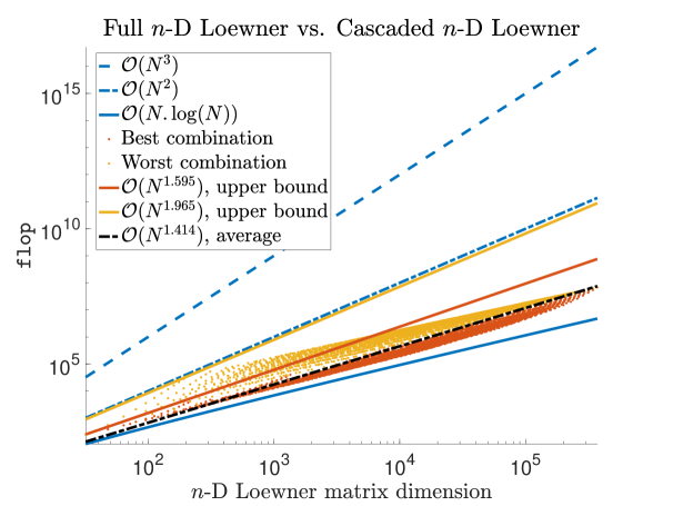
Figure 1: flop comparison. Cascaded $\ord$-D Loewner best and worst combination are respectively materialized by red and yellow dots. An upper bound of the best and worst combination is given with the red and yellow lines. The average complexity is materialized by the dash-dotted black line. Full $\ord$-D Loewner is ${\cal O}(N^{3})$ (blue dashed). Comparison with ${\cal O}(N^{2})$ and ${\cal O}(N\log(N))$ references are shown in dash-dotted and solid blue lines.

6 Data-driven multivariate model construction

Now the theoretical contributions have been detailed, this section will now focus on the numerical aspects and considerations to construct the realization from data measurements.

6.1 Two algorithms

In what follows, we provide details to the proposed two algorithms. The first one is a direct method (without requiring any sort of iteration) inspired by the procedure in [34], while the second is iterative, inspired by the p-AAA algorithm introduced in [48]. These two procedures are outlined in algorithm 1 and algorithm 2. For additional, more in-depth details, we refer the reader to the corresponding works [34, 48].

0:  $\textbf{tab}_{\ord}$ as in Table 2

1:  Check that interpolation points are disjoints.

2:  Compute $d_{j}=\max_{k}{\mathbf{rank~{}}}\mathbb{L}_{1}^{(k)}$, the order along variable $\mathstrut{}^{j}s$ ($k$ being all possible combinations for frozen the variables $\{\mathstrut^{1}s,\cdots,\mathstrut^{k-1}s,\mathstrut^{k+1}s,\cdots,\mathstrut^{\ord}s\}$).

3:  Construct eq. 24, a sub-selection $P_{c}^{(\ord)}$ where $(k_{1},k_{2}\dots,k_{\ord})=(d_{1},d_{2},\dots,d_{\ord})+1$; and $P_{r}^{(\ord)}$ where $(q_{1},q_{2}\dots,q_{\ord})$ gather the rest of the data.

4:  Compute ${\mathbf{c}}_{\ord}$, the $\ord$-D Loewner matrix null space e.g. using Theorem 5.3.

5:  Construct ${\mathbb{A}^{\textrm{Lag}}}$, ${\mathbb{B}^{\textrm{Lag}}}$, $\boldsymbol{\Gamma}$ and $\boldsymbol{\Delta}$ as in Result 4.3 with any left/right separation.

6:  Construct multivariate realization as in Theorem 2.1.

6:  $\hat{\mathbf{H}}(\mathstrut^{1}s,\dots,\mathstrut^{\ord}s)={\mathbf{W}}\boldsymbol{\Phi}(\mathstrut^{1}s,\mathstrut^{2}s,\dots,\mathstrut^{\ord}s)^{-1}{\mathbf{G}}$ interpolates ${\mathbf{H}}(\mathstrut^{1}s,\mathstrut^{2}s,\dots,\mathstrut^{\ord}s)$ along $P_{c}^{(\ord)}$.

Algorithm 1 Direct data-driven pROM construction

0:  $\textbf{tab}_{\ord}$ as in Table 2 and tolerance $\texttt{tol}>0$

1:  Check that interpolation points are disjoints.

2:  while $\texttt{error}>\texttt{tol}$ do

3:     Search the point indexes with maximal error (first iteration: pick any set).

4:     Add points in $P_{c}^{(\ord)}$ and put the remaining ones in $P_{r}^{(\ord)}$, obtain eq. 24.

5:     Compute ${\mathbf{c}}_{\ord}$, the $\ord$-D Loewner matrix null space e.g. using Theorem 5.3.

6:     Construct ${\mathbb{A}^{\textrm{Lag}}}$, ${\mathbb{B}^{\textrm{Lag}}}$, $\boldsymbol{\Gamma}$ and $\boldsymbol{\Delta}$ as in Result 4.3 with any left/right separation.

7:     Construct multivariate realization as in Theorem 2.1.

8:     Evaluate $\texttt{error}=\max||\widehat{\textbf{tab}_{\ord}}-\textbf{tab}_{\ord}||$ where $\widehat{\textbf{tab}_{\ord}}$ is the evaluation of $\hat{\mathbf{H}}(\mathstrut^{1}s,\dots,\mathstrut^{\ord}s)$ along the support points.

9:  end while

9:  $\hat{\mathbf{H}}(\mathstrut^{1}s,\dots,\mathstrut^{\ord}s)={\mathbf{W}}\boldsymbol{\Phi}(\mathstrut^{1}s,\mathstrut^{2}s,\dots,\mathstrut^{\ord}s)^{-1}{\mathbf{G}}$ interpolates ${\mathbf{H}}(\mathstrut^{1}s,\mathstrut^{2}s,\dots,\mathstrut^{\ord}s)$ along $P_{c}^{(\ord)}$.

Algorithm 2 Adaptive data-driven pROM construction

6.2 Discussion

The main difference between the two algorithms is that Algorithm 1 is direct while Algorithm 2 is iterative. Indeed, in the former case, the order is estimated at step 2 while the order is iteratively increased in the latter case until a given accuracy is reached.

By analyzing Algorithm 1, the process first needs to estimate the rational order along each variable $\mathstrut{}^{j}s$. Then, we construct the interpolation set eq. 24 (here one may shuffle data and interpolate different blocks). From this initial data set, the $\ord$-D Loewner matrix and its null space may be computed using either the full (Section 4) or the 1-D recursive (Section 5) approach. Based on the barycentric weights, the realization is constructed using Result 4.3.

By considering algorithm 2, the process is almost similar. The difference between the two algorithms consists in the absence of the order detection process in the second algorithm. It is instead replaced by an evaluation of the model along the data set at each step until a tolerance is reached. Then, at each iteration, one adds the support points set where the maximal error between the model and the data occurs. This idea is originally exploited in the univariate case of AAA in [43] and its parametric version from [48]; we similarly follow this greedy approach.

6.2.1 Transforming to a real arithmetic setup

All computational steps have been presented using complex data. This is the most straightforward manner to present this generic method. However, in system theory, it is often preferable to deal with real-valued functions in order to preserve the realness of the realization and to allow the time-domain simulations of the differential-algebraic equations. To do so, some assumptions and adaptations must be satisfied. Basically, interpolation points along each variable must be either real or chosen closed by conjugations. Then, by introducing the projection matrix ${\mathbf{J}}=\frac{1}{\sqrt{2}}\left[\begin{array}[]{cc}1&1\\ -\imath&\imath\end{array}\right]$ and by repeating it as many times as the complex conjugated points are given, allows to construct left and right projectors that preserves the realness of the $\ord$-D Loewner matrix and thus of the null space. For space limitations, we keep a rigorous exposition of the details for later communication. For more details on the exact procedure, we refer the reader to [34, Section A.2].

6.2.2 Null space computation remarks

To apply the proposed methods to a broad range of real-life applications, we want to comment on the major computational effort / hard point in the proposed process: the null space computation. Indeed, either in the full $\ord$-D and the recursive $1$-D case, a null space must be computed. Numerically, there exist multiple ways to compute it: SVD or QR decomposition, linear resolution… Without entering into details out of the scope of this paper, many tuning variables may be adjusted to improve the accuracy. These elements are crucial to the success of the proposed solution. Investigations are left (and not forgiven) to future works. In the next section, all null spaces have been computed using the standard SVD routine of Matlab. For more details, the reader may refer to [28].

7 Numerical experiments

The effectiveness of the numerical procedures sketched in algorithm 1 and algorithm 2 is illustrated in this section, through some complex examples, involving multiple variables ranging from two to twenty. In what follows the computations have been performed on an Apple MacBook Air with 512 Go SSD and 16 Go RAM, with a M1 chip. The software used is Matlab 2022b.

7.1 A simple synthetic parametric model (2-D)

Let start with the simple example used in [34, Section 5.1] and [48, Section 3.2.1], which transfer function reads: ${\mathbf{H}}(s,p)=\frac{1}{1+25(s+p)^{2}}+\frac{0.5}{1+25(s-0.5)^{2}}+\frac{0.1}{p+25}$. We use the same sampling setting as in the above references. Along the $s$ variable, 21 points linearly spaced points from $[-1,1]$. For the direct method of Algorithm 1 we alternatively sample the grid as $\mathstrut{}^{1}\lambda_{j_{1}}=[-1,-0.8,\cdots,1]$ and $\mathstrut{}^{1}\mu_{i_{1}}=[-0.9,-0.7,\cdots,0.9]$; Then, along the $p$ variable, 21 points linearly spaced points from $[0,1]$. For the direct method of Algorithm 1 we alternatively sample the grid as $\mathstrut{}^{2}\lambda_{j_{2}}=[0,0.1,\cdots,1]$ and $\mathstrut{}^{2}\mu_{i_{2}}=[0.05,0.15,\cdots,0.95]$. First, we apply Algorithm 1 and obtain the single variables singular value decay reported in Figure 2 (left), suggesting approximation orders along $(s,p)$ of $(d_{1},d_{2})=(4,3)$, being precisely the one of the equation ${\mathbf{H}}(s,p)$ above. Then, the $2$-D Loewner matrix is constructed and its associated singular values are reported in Figure 2 (right), leading to the full null space and barycentric weights (results follow next).

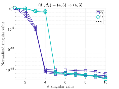
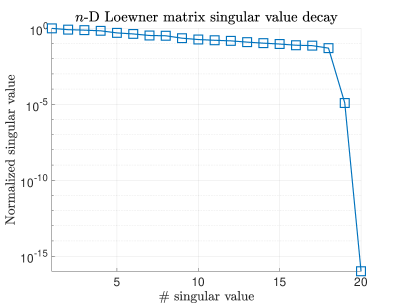
Figure 2: 2-D simple synthetic model: algorithm 1 normalized singular values of each 1-D (left) and the 2-D (right) Loewner matrices.

Next, we investigate the behavior of Algorithm 2. In Table 5, we report the iterations of this algorithm when computing the null space with either the full 2-D version (Table 5(a)) or the recursive 1-D one (Table 5(b)). In both cases, the same order is recovered, i.e. $(4,3)$. Even if the selected interpolation points are slightly different, the final error is below the chosen tolerance i.e. tol=$10^{-6}$. By now comparing the flop  complexity, the benefit of the proposed recursive 1-D approach with respect to the 2-D one is clearly emphasized, even for such a simple setup. Indeed, while the latter is of $9,953$ flop($=1+2^{3}+6^{3}+12^{3}+20^{3}$), the former leads to $680$ flop($=2+10+51+172+445$), being $14$ times smaller.

The mismatch for the three configurations over all the sampling points of $\textbf{tab}_{2}$ data is close to machine precision for all configurations.

(a) algorithm 2 (full $\mathbb{L}_{\ord}$)

Iter.	$\mathstrut{}^{1}\lambda_{j_{1}}$	$\mathstrut{}^{2}\lambda_{j_{2}}$	$(k_{1},k_{2})$	flop
1	$0$	$0$	$(1,1)$	$1^{3}$
2	$-1$		$(2,1)$	$2^{3}$
3	$-0.9$	$0.9$	$(3,2)$	$6^{3}$
4	$-0.1$	$0.2$	$(4,3)$	$12^{3}$
5	$0.6$	$1$	$(5,4)$	$20^{3}$

(b) Algorithm 2 (recursive $\mathbb{L}_{1}$)

$\mathstrut{}^{1}\lambda_{j_{1}}$	$\mathstrut{}^{2}\lambda_{j_{2}}$	$(k_{1},k_{2})$	flop
$0$	$0$	$(1,1)$	2
$-1$		$(2,1)$	10
$0.1$	$0.05$	$(3,2)$	51
$-0.9$	$0.75$	$(4,3)$	172
$0.7$	$0.15$	$(5,4)$	445

Table 5: 2-D simple model iterations with different null space computation methods.

Finally, to conclude this first example, Figure 3 reports the responses (left) and mismatch (right) along $s$ for different values of $p$, for the original model and the obtained ones with algorithm 1 and algorithm 2 (with recursive 1-D null space).

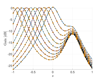
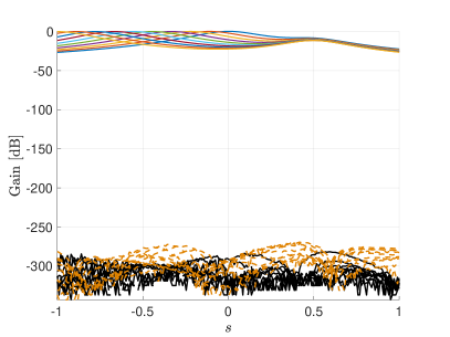
Figure 3: 2-D simple model: frequency responses (left) and errors (right); original vs. algorithm 1 (black lines), and algorithm 2 (orange dots and dashed lines).

7.2 Flutter (3-D)

This numerical example is extracted from industrial data and considers a mixed model/data configuration. It represents the flutter phenomena for flexible aircraft as detailed in [22]. This model can be described as $s^{2}M(m)x(s)+sB(m)x(s)+K(m)x(s)-G(s,v)=u(s)$, where $M(m),B(m),K(m)\in{\mathbb{R}}^{n\times n}$ are the mass, damping, and stiffness matrices, all dependent on the aircraft mass $m\in{\mathbb{R}}_{+}$ ($n\approx 100$). These matrices are constant for a given flight point (but vary for a mass configuration). Then, the generalized aeroelastic forces $G(s,v)\in{\mathbb{C}}^{n\times n}$ describe the aeroelastic forces exciting the structural dynamic. This $G(s,v)$ is known only at a few sampled frequencies and some true airspeed, i.e., $G(\imath\omega_{i},v_{j})$ where $i=1,\cdots,150$ and $j=1,\cdots,10$. Note that these values are obtained through dedicated high-fidelity numerical solvers. The sampling setup is as follows. Along the $s$ variable, $\mathstrut{}^{1}\lambda_{j_{1}}$ are 150 logarithmically spaced points between $\imath[10,35]$ and $\mathstrut{}^{1}\mu_{i_{1}}=-\mathstrut^{1}\lambda_{j_{1}}$; Along the $v$ variable, $\mathstrut{}^{2}\lambda_{j_{2}}$ are 5 linearly spaced points between $[4.77,5.21]\cdot 10^{3}$ and $\mathstrut{}^{2}\mu_{i_{2}}$, 5 linearly spaced between $[4.82,5.27]\cdot 10^{3}$; Along the $m$ variable, $\mathstrut{}^{3}\lambda_{j_{3}}$ are 5 linearly spaced points between $[1.52,1.66]\cdot 10^{3}$ and $\mathstrut{}^{2}\mu_{i_{2}}$, 5 linearly spaced between $[1.54,1.68]\cdot 10^{3}$.

Here, the data is a $3$-dimensional tensor $\textbf{tab}_{3}\in{\mathbb{C}}^{300\times 10\times 10}$. By applying algorithm 1, an approximation order $(14,1,1)$ is reasonable. The singular value decay of the 3-D Loewner matrix is reported in Figure 4 (left). Then, the original and pROM frequency responses are shown in Figure 4 (right), resulting in an accurate model.

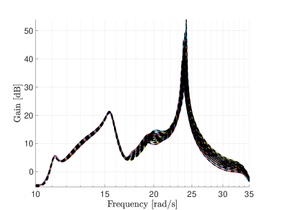
Figure 4: 3-D flutter model: 3-D Loewner matrix singular values (left) and frequency responses (right). Original (solid colored) and pROM (black dashed).

One relevant point of the proposed Loewner framework, nicely illustrated in this application, is its ability to construct a realization of a pROM, based on a hybrid data set, mixing frequency-domain data and matrices. By connecting this problem to NEPs, the parametric rational approximation allows us to estimate the eigenvalue trajectories; we refer to [47, 54, 22] for details and industrial applications.

7.3 A multi-variate function with a high number of variables (20-D)

To conclude and to numerically demonstrate the scalability features of our process, let us consider the following rational function in $20$ variables

$$\small{\mathbf{H}}(\mathstrut^{1}s, \mathstrut{}^{2}s,\ldots,\mathstrut^{20}s)=$$

$$\dfrac{3\cdot\mathstrut^{1}s^{3}+4\cdot\mathstrut^{8}s+\mathstrut^{12}s+\mathstrut^{13}s\cdot\mathstrut^{14}s+\mathstrut^{15}s}{\mathstrut{}^{1}s+\mathstrut^{2}s^{2}\cdot\mathstrut^{3}s+\mathstrut^{4}s+\mathstrut^{5}s+\mathstrut^{6}s+\mathstrut^{7}s\cdot\mathstrut^{8}s+\mathstrut^{9}s\cdot\mathstrut^{10}s\cdot\mathstrut^{11}s+\mathstrut^{13}s+\mathstrut^{13}s^{3}\cdot\pi+\mathstrut^{17}s+\mathstrut^{18}s\cdot\mathstrut^{19}s-\mathstrut^{20}s},$$

with a complexity of $(3,2,1,1,1,1,1,1,1,1,1,1,1,1,1,3,1,1,1,1)$. By applying algorithm 1 with the recursive 1-D null space construction, the barycentric coefficients ${\mathbf{c}}_{\ord}\in{\mathbb{C}}^{6291456}$ are obtained with a computational complexity of 54,263,884 flop, computed in 55 minutes. As provided in the supplementary material, this vector allows reconstructing the original model ${\mathbf{H}}$ with $\hat{\mathbf{H}}$, with an absolute error $\approx 10^{-11}$, for a random parameter selection.

Applying the full $\ord$-D Loewner version instead would have theoretically required the construction of a Loewner matrix of dimension $N=6,291,456$, which null space computation would cost about $2.49\cdot 10^{20}$ flop, being prohibitive, at least on a desktop computer. Note that storing such a $N\times N$ $\ord$-D Loewner matrix would require $6291456^{2}\cdot\frac{8}{2^{30}}=294,912$ GB in double precision and $147,456$ GB in simple precision (where $8$ is the number of bytes in double precision and $2^{30}$ scales the bytes into Giga Bytes). Here, constructing the complete 20-D tensor is a waste of time and energy. Instead, we consider that the unknown function ${\mathbf{H}}$ can be evaluated when needed.

8 Conclusions

We investigated the Loewner framework for linear multivariate/parametric systems and developed a complete methodology (and two algorithms) for data-driven $\ord$ variable pROM realization construction, in the ($\ord$-D) Loewner framework. We also showed the relationship between $\ord$-D Loewner and Sylvester equations. Then, as the numerical complexity explodes with the number of data and variables, we introduce a recursive 1-D null space procedure, equivalent to the full $\ord$-D one. This process reduces the complexity from ${\cal O}(N^{3})$ to approximately ${\cal O}(N^{1.4})$. This becomes a major step toward taming the curse of dimensionality. Throughout the paper we apply these results to some numerical examples, demonstrating their effectiveness. Last but not least, we claim that the contributions presented are not limited to the system dynamic and rational approximation fields, but rather apply to many scientific computing domains, including tensor approximation and nonlinear eigenvalue problems, for which dimensionality remains an issue.

Supplementary material

This contribution presents the main theoretical results, emphasizing technical details and procedures supported by some numerical experiments. To provide an exhaustive account of our findings (in the direction of applying the proposed approaches for a multitude of test cases) with more insight for interested readers, additional numerical results are made available at

https://sites.google.com/site/charlespoussotvassal/nd_loew_tcod

This web page gathers a collection of benchmarks that numerically demonstrate the scalability of the proposed algorithms. It also includes the model description, the associated $n$-D tensor (if accessible), and the obtained solutions, allowing reproducibility of the results in the paper.

References

- [1] Amsallem, D., Farhat, C.: An online method for interpolating linear parametric reduced-order models. SIAM J. Sci. Comput. 33(5), 2169–2198 (2011). 10.1137/100813051
- [2] Andreuzzi, F., Demo, N., Rozza, G.: A dynamic mode decomposition extension for the forecasting of parametric dynamical systems. SIAM J. Appl. Dyn. Syst. 22(3), 2432–2458 (2023). 10.1137/22M1481658
- [3] Antoulas, A.C.: Approximation of Large-Scale Dynamical Systems, Adv. Des. Control, vol. 6. SIAM Publications, Philadelphia, PA (2005). 10.1137/1.9780898718713
- [4] Antoulas, A.C., Anderson, B.D.O.: On the scalar rational interpolation problem. IMA J. Math. Control. Inf. 3(2-3), 61–88 (1986). 10.1093/imamci/3.2-3.61
- [5] Antoulas, A.C., Beattie, C.A., Gugercin, S.: Interpolatory Methods for Model Reduction. Computational Science & Engineering. Society for Industrial and Applied Mathematics, Philadelphia, PA (2020). 10.1137/1.9781611976083
- [6] Antoulas, A.C., Ionita, A.C., Lefteriu, S.: On two-variable rational interpolation. Linear Algebra and its Applications 436(8), 2889–2915 (2012). 10.1016/j.laa.2011.07.017. Special Issue dedicated to Danny Sorensen’s 65th birthday
- [7] Antoulas, A.C., Lefteriu, S., Ionita, A.C.: A tutorial introduction to the Loewner framework for model reduction. In: Model Reduction and Approximation, chap. 8, pp. 335–376. SIAM (2017). doi/10.1137/1.9781611974829.ch8
- [8] Austin, A.P., Krishnamoorthy, M., Leyffer, S., Mrenna, S., Müller, J., Schulz, H.: Practical algorithms for multivariate rational approximation. Computer Physics Communications 261, 107663 (2021). 10.1016/j.cpc.2020.107663
- [9] Baur, U., Beattie, C., Benner, P., Gugercin, S.: Interpolatory projection methods for parameterized model reduction. SIAM J. Comput. 33(5), 2489–2518 (2011)
- [10] Baur, U., Benner, P., Feng, L.: Model order reduction for linear and nonlinear systems: A system-theoretic perspective. Archives of Computational Methods in Engineering 21(4), 331–358 (2014). 10.1007/s11831-014-9111-2
- [11] Beltrán-Pulido, A., Bilionis, I., Aliprantis, D.: Physics-informed neural networks for solving parametric magnetostatic problems. IEEE Transactions on Energy Conversion 37(4), 2678–2689 (2022). 10.1109/TEC.2022.3180295
- [12] Benner, P., Grivet-Talocia, S., Quarteroni, A., Rozza, G., Schilders, W., Silveira, L.M.: Model Order Reduction, Volume 1: System- and Data-Driven Methods and Algorithms. De Gruyter, Berlin, Boston (2021). 10.1515/9783110498967. URL https://doi.org/10.1515/9783110498967
- [13] Benner, P., Grivet-Talocia, S., Quarteroni, A., Rozza, G., Schilders, W., Silveira, L.M.: Model Order Reduction, Volume 2: Snapshot-Based Methods and Algorithms. De Gruyter, Berlin, Boston (2021). 10.1515/9783110671490. URL https://doi.org/10.1515/9783110671490
- [14] Benner, P., Gugercin, S., Willcox, K.: A survey of projection-based model reduction methods for parametric dynamical systems. SIAM Rev. 57(4), 483–531 (2015). 10.1137/130932715
- [15] Berrut, J.P., Trefethen, L.N.: Barycentric Lagrange interpolation. SIAM Review 46(3), 501–517 (2004). 10.1137/S00361445024177
- [16] Bradde, T., Grivet-Talocia, S., Zanco, A., Calafiore, G.C.: Data-driven extraction of uniformly stable and passive parameterized macromodels. IEEE Access 10, 15786–15804 (2022). 10.1109/ACCESS.2022.3147034
- [17] Brennan, M.C., Embree, M., Gugercin, S.: Contour integral methods for nonlinear eigenvalue problems: A systems theoretic approach. SIAM Rev. 65(2), 439–470 (2023). 10.1137/20M1389303
- [18] Chellappa, S., Feng, L., de la Rubia, V., Benner, P.: Adaptive interpolatory MOR by learning the error estimator in the parameter domain. Model Reduction of Complex Dynamical Systems pp. 97–117 (2021). 10.1007/978-3-030-72983-7_5
- [19] Constantine, P.G.: Active subspaces: Emerging ideas for dimension reduction in parameter studies. SIAM (2015). 10.1137/1.9781611973860
- [20] Debals, O., Van Barel, M., De Lathauwer, L.: Löwner-based blind signal separation of rational functions with applications. IEEE Transactions on Signal Processing 64(8), 1909–1918 (2015). 10.1109/TSP.2015.2500179
- [21] Demo, N., Strazzullo, M., Rozza, G.: An extended physics informed neural network for preliminary analysis of parametric optimal control problems. Computers & Mathematics with Applications 143, 383–396 (2023). 10.1016/j.camwa.2023.05.004
- [22] dos Reis de Souza, A., Poussot-Vassal, C., Vuillemin, P., Zucco, J.T.: Aircraft flutter suppression: from a parametric model to robust control. In: Proceedings of European Control Conference. Bucharest, Romania (2023). 10.23919/ECC57647.2023.10178141
- [23] Geuss, M., Lohmann, B.: STABLE - a stability algorithm for parametric model reduction by matrix interpolation. Mathematical and Computer Modelling of Dynamical Systems 22(4), 307–322 (2016). 10.1080/13873954.2016.1198383
- [24] Gosea, I.V., Gugercin, S.: Data-driven modeling of linear dynamical systems with quadratic output in the AAA framework. Journal of Scientific Computing 91(1), 16 (2022). 10.1007/s10915-022-01771-5
- [25] Gosea, I.V., Gugercin, S., Unger, B.: Parametric model reduction via rational interpolation along parameters. In: 60th IEEE Conference on Decision and Control (CDC), December 14–17, Austin, TX, USA, pp. 6895–6900 (2021). 10.1109/CDC45484.2021.9682841
- [26] Gosea, I.V., Poussot-Vassal, C., Antoulas, A.: Data-driven modeling and control of large-scale dynamical systems in the Loewner framework. Handbook of Numerical Analysis 23(Numerical Control: Part A), 499–530 (2022). 10.1016/bs.hna.2021.12.015
- [27] Grasedyck, L., Kressner, D., Tobler, C.: A literature survey of low-rank tensor approximation techniques. GAMM-Mitteilungen 36(1), 53–78 (2013). 10.1002/gamm.201310004
- [28] Guglielmi, N., Overton, M., Stewart, G.: An efficient algorithm for computing the generalized null space decomposition. SIAM J. Matrix Anal. Appl. 36(1), 38–54 (2015). 10.1137/140956737
- [29] Guo, M., Manzoni, A., Amendt, M., Conti, P., Hesthaven, J.S.: Multi-fidelity regression using artificial neural networks: Efficient approximation of parameter-dependent output quantities. Computer methods in applied mechanics and engineering 389, 114378 (2022). 10.1016/j.cma.2021.114378
- [30] Güttel, S., Negri Porzio, G.M., Tisseur, F.: Robust rational approximations of nonlinear eigenvalue problems. SIAM J. Comput. 44(4), A2439–A2463 (2022). 10.1137/20M1380533
- [31] Güttel, S., Van Beeumen, R., Meerbergen, K., Michiels, W.: NLEIGS: A class of fully rational Krylov methods for nonlinear eigenvalue problems. SIAM J. Comput. 36(6), A2842–A2864 (2014). 10.1137/130935045
- [32] Hesthaven, J.S., Rozza, G., Stamm, B.: Certified Reduced Basis Methods for Parametrized Partial Differential Equations. SpringerBriefs in Mathematics. Springer, Cham (2016). 10.1007/978-3-319-22470-1
- [33] Hund, M., Mitchell, T., Mlinarić, P., Saak, J.: Optimization-based parametric model order reduction via first-order necessary conditions. SIAM J. Sci. Comput. 44(3), A1554–A1578 (2022). 10.1137/21M140290X
- [34] Ionita, A., Antoulas, A.: Data-Driven Parametrized Model Reduction in the Loewner Framework. SIAM J. Sci. Comput. 36(3), A984–A1007 (2014). 10.1137/130914619
- [35] Karachalios, D.S., Gosea, I.V., Antoulas, A.C.: The Loewner framework for system identification and reduction. In: P. Benner, S. Grivet-Talocia, A. Quarteroni, G. Rozza, W.H.A. Schilders, L.M. Silveira (eds.) Methods and Algorithms, Handbook on Model Reduction, vol. 1. De Gruyter (2021). 10.1515/9783110498967-006
- [36] Kolda, T.G., Bader, B.W.: Tensor decompositions and applications. SIAM Rev. 51(3), 455–500 (2009). 10.1137/07070111X
- [37] Lietaert, P., Meerbergen, K., Pérez, J., Vandereycken, B.: Automatic rational approximation and linearization of nonlinear eigenvalue problems. IMA Journal of Numerical Analysis 42(2), 1087–1115 (2022). 10.1093/imanum/draa098
- [38] Loewner, K.: Über monotone Matrixfunktionen. Mathematische Zeitschrift 38(1), 177–216 (1934). 10.1007/BF01170633
- [39] Mayo, A.J., Antoulas, A.C.: A framework for the solution of the generalized realization problem. Linear Algebra and Its Applications 425(2-3), 634–662 (2007). 10.1016/j.laa.2007.03.008
- [40] McQuarrie, S.A., Khodabakhshi, P., Willcox, K.E.: Nonintrusive reduced-order models for parametric partial differential equations via data-driven operator inference. SIAM J. Sci. Comput. 45(4), A1917–A1946 (2023). 10.1137/21M1452810
- [41] Mlinarić, P., Benner, P., Gugercin, S.: Interpolatory necessary optimality conditions for reduced-order modeling of parametric linear time-invariant systems. arXiv preprint arXiv:2401.10047 (2024). 10.48550/arXiv.2401.10047
- [42] Mlinarić, P., Rave, S., Saak, J.: Parametric model order reduction using pyMOR. Model Reduction of Complex Dynamical Systems pp. 357–367 (2021). 10.1007/978-3-030-72983-7_17
- [43] Nakatsukasa, Y., Sète, O., Trefethen, L.N.: The AAA algorithm for rational approximation. SIAM J. Comput. 40(3), A1494–A1522 (2018). 10.1137/16M1106122
- [44] Nakatsukasa, Y., Sete, O., Trefethen, L.N.: The first five years of the AAA algorithm. ArXiv preprint online (2023). 10.48550/arXiv.2312.03565
- [45] Nobile, F., Pradovera, D.: Non-intrusive double-greedy parametric model reduction by interpolation of frequency-domain rational surrogates. ESAIM: Mathematical Modelling and Numerical Analysis 55(5), 1895–1920 (2021). 10.1051/m2an/2021040
- [46] Peherstorfer, B., Willcox, K.: Data-driven operator inference for nonintrusive projection-based model reduction. Computer Methods in Applied Mechanics and Engineering 306, 196–215 (2016). 10.1016/j.cma.2016.03.025
- [47] Quero, D., Vuillemin, P., Poussot-Vassal, C.: A generalized eigenvalue solution to the flutter stability problem with true damping: the p-L method. Journal of Fluids and Structures 103, 103266 (2021). 10.1016/j.jfluidstructs.2021.103266
- [48] Rodriguez, A.C., Balicki, L., Gugercin, S.: The p-AAA algorithm for data driven modeling of parametric dynamical systems. SIAM J. Sci. Comput. 45(3), A1332–A1358 (2023). 10.1137/20M1322698
- [49] Sun, S., Feng, L., Chan, H.S., Miličić, T., Vidaković-Koch, T., Benner, P.: Parametric dynamic mode decomposition for nonlinear parametric dynamical systems. arXiv preprint arXiv:2305.06197 (2023). 10.48550/arXiv.2305.06197
- [50] Tu, J.H., Rowley, C.W., Luchtenburg, D.M., Brunton, S.L., Kutz, J.N.: On dynamic mode decomposition: Theory and applications. Journal of Computational Dynamics 1(2), 391–421 (2014). 10.3934/jcd.2014.1.391
- [51] Van Dooren, P., Gallivan, K.A., Absil, P.A.: -optimal model reduction of MIMO systems. Applied Mathematics Letters 21(12), 53–62 (2008)
- [52] Verbeke, D., Ishteva, M., Dreesen, P.: MIMO transfer function decoupling by Loewner tensorization. IFAC-PapersOnLine 56(2), 7300–7305 (2023). 10.1016/j.ifacol.2023.10.342
- [53] Vervliet, N., Debals, O., Sorber, L., De Lathauwer, L.: Breaking the curse of dimensionality using decompositions of incomplete tensors: Tensor-based scientific computing in big data analysis. IEEE Signal Processing Magazine 31(5), 71–79 (2014). 10.1109/MSP.2014.2329429
- [54] Vojkovic, T., Quero, D., Poussot-Vassal, C., Vuillemin, P.: Low-order parametric state-space modeling of MIMO systems in the Loewner framework. SIAM J. Appl. Dyn. Syst. 22(4), 3130–3164 (2023). 10.1137/22M1509898
- [55] Vuillemin, P., Kergus, P., Poussot-Vassal, C.: Hybrid Loewner data driven control. In: Proceedings of the IFAC World Congress. Berlin, Germany (2020). 10.1016/j.ifacol.2020.12.1574
- [56] Xiao, Y.Q., Grivet-Talocia, S., Manfredi, P., Khazaka, R.: A novel framework for parametric Loewner matrix interpolation. IEEE Transactions on Components, Packaging and Manufacturing Technology 9(12), 2404–2417 (2019). 10.1109/TCPMT.2019.2948802
- [57] Yıldız, S., Goyal, P., Benner, P., Karasözen, B.: Learning reduced-order dynamics for parametrized shallow water equations from data. International Journal for Numerical Methods in Fluids 93(8), 2803–2821 (2021). 10.1002/fld.4998
- [58] Yue, Y., Feng, L., Benner, P.: Reduced-order modelling of parametric systems via interpolation of heterogeneous surrogates. Advanced Modeling and Simulation in Engineering Sciences 6, 10 (2019). 10.1186/s40323-019-0134-y
- [59] Zanco, A., Grivet-Talocia, S., Bradde, T., De Stefano, M.: Enforcing passivity of parameterized LTI macromodels via Hamiltonian-driven multivariate adaptive sampling. IEEE Trans. on Computer-Aided Design of Integrated Circ. and Sys. 39(1), 225–238 (2018). 10.1109/TCAD.2018.2883962