GOLD: Geometry Problem Solver with Natural Language Description

Abstract

Addressing the challenge of automated geometry math problem-solving in artificial intelligence (AI) involves understanding multi-modal information and mathematics. Current methods struggle with accurately interpreting geometry diagrams, which hinders effective problem-solving. To tackle this issue, we present the Geometry problem sOlver with natural Language Description (GOLD) model. GOLD enhances the extraction of geometric relations by separately processing symbols and geometric primitives within the diagram. Subsequently, it converts the extracted relations into natural language descriptions, efficiently utilizing large language models to solve geometry math problems. Experiments show that the GOLD model outperforms the Geoformer model, the previous best method on the UniGeo dataset, by achieving accuracy improvements of 12.7% and 42.1% in calculation and proving subsets. Additionally, it surpasses the former best model on the PGPS9K and Geometry3K datasets, PGPSNet, by obtaining accuracy enhancements of 1.8% and 3.2%, respectively.

1 Introduction

Automated solving of geometry math problems has gained considerable attention in the AI community recently Chen et al. (2021); Lu et al. (2021); Cao and Xiao (2022); Chen et al. (2022); Zhang et al. (2023); Peng et al. (2023); Ning et al. (2023). Unlike math word problems, geometry math problems involve additional geometry diagrams, necessitating comprehensive reasoning capabilities for understanding multi-modal information (refer to Figure 1 for an example of a geometry math problem). As a result, research on automated geometry math problem solving is still in its infancy Chen et al. (2022).

Existing approaches for solving geometry math problems utilize neural networks to embed the diagram and problem text separately or jointly, resulting in highly generalized models Chen et al. (2021, 2022). However, these methods struggle with accurately capturing the complex relationships within geometry diagrams Lu et al. (2023b). Additionally, their vector-based representation of geometric relations is not easily interpretable by humans, posing challenges in identifying whether performance issues are from the relation extraction or the problem-solving component. In a different approach, some studies have successfully translated geometry diagrams into formal languages, enhancing precision and interpretability Sachan et al. (2017); Seo et al. (2015); Lu et al. (2021); Zhang et al. (2023). However, these methods do not separately process relations among geometric primitives and relations between symbols and geometric primitives, which adds difficulty in solving the geometry math problem correctly. Moreover, these approaches necessitate specifically designed solvers that take formal languages as input, making them incompatible with prevalent large language models (LLMs).

To address the limitations of existing methods in solving geometry math problems, we introduce the GOLD model. The GOLD model converts geometry diagrams into natural language descriptions, aiding in the generation of solution programs for the problems. Particularly, the GOLD model’s relation-construction head extracts two types of geometric relations: sym2geo (relations between symbols and geometric primitives) and geo2geo (relations among geometric primitives). This process involves two specialized heads that separately model symbols and geometric primitives within diagrams as distinct vectors. These extracted geometric relations are then converted into natural language descriptions. This not only improves the model’s interpretability but also connects geometry diagrams with problem texts. Furthermore, since these natural language descriptions meet the input requirements of LLMs, the GOLD model is able to utilize the advanced LLMs as the problem-solving module, efficiently generating solution programs used to solve geometry math problems.

To evaluate the effectiveness of the GOLD model, we conduct experiments on the three latest released datasets: UniGeo (comprising calculation and proving subsets) Chen et al. (2022), PGPS9K Zhang et al. (2023), and Geometry3K Lu et al. (2021). The experimental results show the significant performance gains of our GOLD model compared to state-of-the-art (SOTA) models. It surpasses the Geoformer model, which is the SOTA model on the UniGeo dataset, by 12.7% and 42.1% in accuracy on the UniGeo calculation and proving subsets, respectively. Additionally, our GOLD model outperforms the PGPSNet model, the SOTA model on the PGPS9K and Geometry3K datasets by 1.8% and 3.2% in accuracy, respectively. These results highlight the superior performance and effectiveness of our proposed GOLD model compared to existing approaches.

The contributions of this work are: (1) We propose the GOLD model to extract geometric relations from geometry diagrams and subsequently convert these relations into natural languages, which are then utilized for solving geometry math problems. Its compatibility with LLMs is a significant advantage, enabling the GOLD model to utilize the capabilities of LLMs to generate solution programs. (2) The GOLD model separately processes symbols and geometric primitives from the diagrams. This separation design simplifies the extraction of the geometric relations. (3) Our GOLD model demonstrates significant improvements over previous methods across all evaluated datasets, validating the effectiveness of our approach.

2 Related Work

Early works have explored solving geometry math problems through rule-based approaches Gelernter et al. (1960); Wen-Tsün (1986); Chou and Gao (1996a, b). Recently, with the success of deep learning methods, several works have explored using neural network architectures for automated geometry math problem-solving. Approaches such as NGS Chen et al. (2021) utilizing LSTM Hochreiter and Schmidhuber (1997) and ResNet-101 He et al. (2016) encoded problem texts and geometry diagrams separately. Later, methods like DPE-NGS Cao and Xiao (2022) replaced the text encoder with transformer models. However, these methods struggle to effectively integrate problem texts and geometry diagrams. In response, Geoformer Chen et al. (2022) emerged, embedding both diagram and problem text jointly using the VL-T5 Cho et al. (2021) model, treating visuals as additional tokens. Despite these advancements, they still struggle to provide precise descriptions of slender, overlapped geometric primitives with complex spatial relationships Zhang et al. (2022), resulting in sub-optimal performance when solving geometry math problems.

Other approaches typically involve parsing the diagram into formal language and utilizing specific solvers to generate solution programs. Recent works like Inter-GPS Lu et al. (2021) and PGPSNet Zhang et al. (2023) employed their parsers to describe the diagram using carefully crafted rules. However, these methods based on predefined rules often lack extensibility, resulting in limited generalization capabilities. To address this issue, our proposed GOLD model generates natural language descriptions of the diagrams, ensuring compatibility of adopting LLMs to generate solution programs.

3 Model

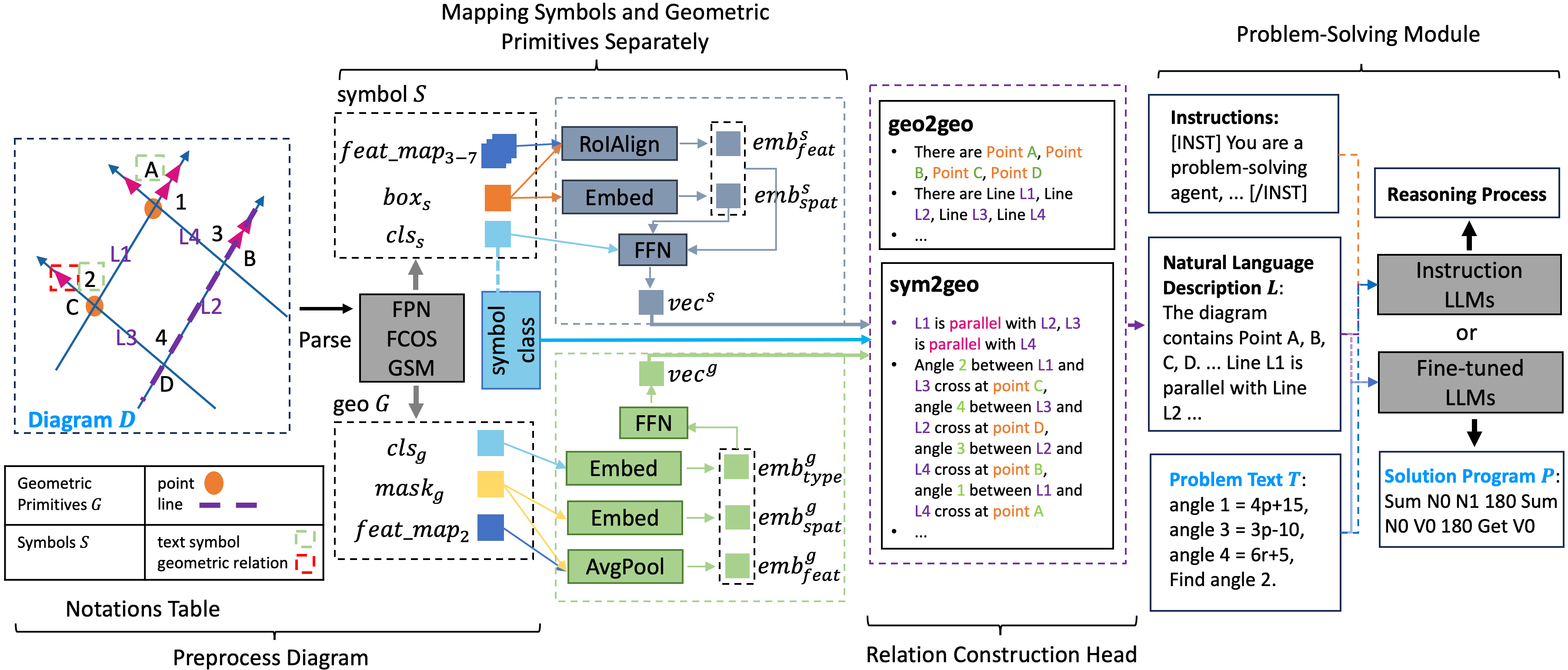
Figure 1: The illustration of the GOLD Model. The diagram $\mathcal{D}$, problem text $\mathcal{T}$, and solution program $\mathcal{P}$ used in this illustration are sourced from the PGPS9K dataset (Zhang et al., 2023). The symbols and geometric primitives in the diagram are annotated using the notations from the Notation Table, which are consistent with the colours of extracted relations of sym2geo and geo2geo.

Our GOLD model is illustrated in Figure 1.

3.1 Task Description and Pre-parsing

The objective is to generate the correct solution program $\mathcal{P}$ to solve the problem by analyzing a geometry math problem text $\mathcal{T}$ and its corresponding diagram $\mathcal{D}$. Specifically, the solution program represents intermediate steps in the domain-specific language generating the output for the question (see an example of solution program in Figure 1).

In our approach, we initially preprocess geometry diagrams to extract geometric primitives $\mathcal{G}$ (including Point P, Line L, and Circle C) and symbols $\mathcal{S}$ from the diagram $\mathcal{D}$ for subsequent task. Specifically, we utilize a standard Feature Pyramid Network (FPN) Lin et al. (2017) integrated with a MobileNetV2 Sandler et al. (2018) backbone for this task. For the detection of symbols, we apply the anchor-free detection model FCOS Tian et al. (2022), and for the extraction of geometric primitives, we use the GSM model Zhang et al. (2022). The FCOS model employs feature maps P3 to P7, generated by the FPN layer, to detect symbols within the diagram. This detection step produces bounding box coordinates ($\text{box}_{s}$) and class type ($\text{cls}_{s}$) for each symbol ($s\in\mathcal{S}$). For the extraction of geometric primitives, we prefer using the feature map P2 instead of P1, as P2 is more memory-efficient due to its lower resolution. This process results in the identification of segmentation masks $(\text{mask}_{g}$) and class type ($\text{cls}_{g}$) for each geometric primitive ($g\in\mathcal{G}$).

3.2 Mapping Symbols and Geometric Primitives Separately

Before constructing the geometric relations, we map the symbols and geometric primitives into vectors. To achieve this, we introduce two heads: symbol vector head and geometric primitive vector head. Specifically, each head functions as extracting the feature_embedding ($\text{emb}_{\mathit{feat}}$) and spatial_embedding ($\text{emb}_{\mathit{spat}}$). The feature_embedding is computed from the cropped feature map, which is determined by either the bounding box or the segmentation mask. Moreover, where symbols and geometric primitives are placed significantly shapes how they relate. For instance, only points lying on a line can hold the geometric relation with that particular line. Thus, we hypothesize that incorporating spatial information of $\mathcal{S}$ and $\mathcal{G}$ can enhance the accuracy of predictions about geometric relations. Consequently, we embed the bounding boxes of symbols and the coordinates of the geometric primitives into the spatial_embedding.

3.2.1 Constructing the  feature_embedding

To obtain the feature_embedding ($\text{emb}^{s,g}_{\mathit{feat}}$) and spatial_embedding ($\text{emb}^{s,g}_{\mathit{spat}}$) for symbol $s$ or geometric primitive $g$, we conduct the below calculation:

$$\text{emb}^{s,g}_{\mathit{feat}}=\text{ReLU}(\mathbf{W}^{s,g}_{\mathit{feat}}\mathbf{V}^{s,g})$$ (1)

where $\mathbf{W}^{s,g}_{\mathit{feat}}\in\mathbb{R}^{h\times h}$ are trainable parameters for either symbols or geometric primitives. Next, we elaborate the calculation process of $\mathbf{V}^{s,g}$ for symbols and geometric primitives separately.

To obtain the $\mathbf{V}^{s}$ for symbol $s$, we utilize RoIAlign He et al. (2017) on its feature map, based on the bounding box of symbol $s$:

$$\mathbf{V}^{s}=\mathbb{F}(\text{ReLU}(\text{BN}(\text{Conv}(\text{RoIAlign}(\text{box}_{s},\text{feat\_map}_{i})))))$$ (2)

where $i$ refers to the $i$-th layer of feature maps where the bounding box ($\text{box}_{s}$) is calculated from. The Conv is the convolution layer with 64 channels, BN is the BatchNorm layer, and ReLU is the ReLU activation layer. The $\mathbb{F}$ means flatten operation, indicating that the $\mathbf{V}^{s}$ is further flatten into a vector and used for obtaining the feature_embedding $\text{emb}^{s}_{feat}$ for symbol $s$ through Eq 1.

To obtain the $\mathbf{V}^{g}$ for geometric primitive $g$, we perform an element-wise multiplication between the segmentation mask $(\text{mask}_{g}$) of $g$ and the P2 layer of feature map $(\text{feat\_map}_{2}$). Next, we flatten the resulting vector along the height and width dimensions and apply global average pooling to obtain the $\mathbf{V}^{g}$:

$$\mathbf{V}^{g}=\text{AvgPool}(\mathbb{F}(\text{mask}_{g}\times\text{feat\_map}_{2}))$$ (3)

The $\mathbf{V}^{g}$ is used for calculating the feature_embedding $\text{emb}^{g}_{feat}$ for geometric primitive $g$ through Eq 1.

3.2.2 Constructing the  spatial_embedding

The spatial_embedding is obtained by mapping the spatial information of symbols and geometric primitives into embeddings. Specifically, for symbol $s$, we map the coordinates of its bounding box into an embedding using the trainable parameters $\mathbf{W}^{s}_{\mathit{spat}}\in\mathbb{R}^{h\times 4}$. Specifically, $\text{emb}^{s}_{\mathit{spat}}\mathbin{=}\mathbf{W}^{s}_{\mathit{spat}}[x_{t},y_{t},x_{b},y_{b}]^{\top}$, where $(x_{t},y_{t})$ represent the coordinates of the top-left corner of the bounding box, and $(x_{b},y_{b})$ is the coordinates of the bottom-right corner of the bounding box.

Next, to obtain the spatial_embedding of a geometric primitive $g$, we start by representing coordinates of $g$ using $loc_{g}$. The format of $loc_{g}$ depends on the class type ($\text{cls}_{g}$) of the geometric primitive: for a point, it contains two numbers ($n_{g}=2$) representing its coordinates; for a line, it contains four numbers ($n_{g}=4$) representing the coordinates of its start and end points; and for a circle, it contains three numbers ($n_{g}=3$) representing the coordinates of its centre point and the radius length. We then map $loc_{g}$ into spatial_embedding by calculating $\text{emb}^{g}_{\mathit{spat}}=\text{ReLU}(\mathbf{W}^{g}_{\mathit{spat}}(\mathbf{W}^{g}_{\mathit{loc}}loc_{g}$)), where $\mathbf{W}^{g}_{\mathit{loc}}\in\mathbb{R}^{h\times n_{g}}$ are different trainable parameters for different $\text{cls}_{g}$, and $\mathbf{W}^{g}_{\mathit{spat}}\in\mathbb{R}^{h\times h}$ are trainable parameters.

To help the model differentiate between different types of geometric primitives, we introduce the geo_type_embedding ($\text{emb}^{g}_{\mathit{type}}$) to capture the semantic information of the geometric primitive. The $\text{emb}^{g}_{\mathit{type}}$ is obtained by performing a lookup operation on the embeddings using the class type $(\text{cls}_{g}$) of $g$ from the list of geometric primitive types $[\mathbf{P},\mathbf{L},\mathbf{C}]$. Specifically, $\text{emb}^{g}_{\mathit{type}}\mathbin{=}\text{embedding}(\text{cls}_{g})$, where $\text{cls}_{g}$ is the class type ID of $g$.

3.2.3 Symbol Vector and Geometric Primitive Vector

The vector representation $\text{vec}^{s\in{\mathcal{S}}}$ of symbol $s$ is obtained by passing concatenated $\text{emb}^{s}_{\textit{feat}}$ and $\text{emb}^{s}_{\textit{spat}}$ through a specific feed-forward neural network:

$$\text{vec}^{s\in{\mathcal{S}}}=\text{ReLU}(\mathbf{W}^{s}_{\mathit{vec}}[\text{emb}^{s}_{\mathit{feat}}:\text{emb}^{s}_{\mathit{spat}}]^{\top})$$ (4)

where $\mathbf{W}^{s}_{\mathit{vec}}\in\mathbb{R}^{h\times 2h}$ are the trainable parameters depending on the class type ($\text{cls}_{s}$) of symbol $s$, and $[:]$ refers to concatenation operation.

The vector representation of the geometric primitive $\text{vec}^{g\in{\mathcal{G}}}$ is obtained by summing up three embeddings relevant to the geometric primitive $g$, $\text{emb}^{g}_{\mathit{feat}}$, $\text{emb}^{g}_{\mathit{spat}}$, and $\text{emb}^{g}_{\mathit{type}}$:

$$\text{vec}^{g\in{\mathcal{G}}}=\text{ReLU}(\mathbf{W}^{g}_{\mathit{vec}}(\text{emb}^{g}_{\mathit{feat}}+\text{emb}^{g}_{\mathit{spat}}+\text{emb}^{g}_{\mathit{type}}))$$ (5)

where $\mathbf{W}^{g}_{\mathit{vec}}\in\mathbb{R}^{h\times h}$ are the trainable parameters.

3.3 Relation Construction Head

The relation-construction head aims to establish sym2geo relations among symbols and geometric primitives and geo2geo relations among geometric primitives themselves.

3.3.1 sym2geo relation

The sym2geo relation can be further divided into text2geo and other2geo relations. The text2geo relation explains the association between text symbols and geometric primitives, where the text symbols are used to be the reference to a geometric primitive or to display degree, length, etc. To distinguish the role of a text symbol, we introduce the text_class for the text symbol. Specifically, when text_class is category $\mathit{0}$, the text2geo signifies point (or line, or circle) names; when text_class is category $\mathit{1}$, the text2geo corresponds to angle degrees; when text_class is category $\mathit{2}$, the text2geo signifies line lengths; when text_class is category $\mathit{3}$, the text2geo denotes the degree of an angle within a circle. The probabilities of the category ($P(\textit{text\_class}|s)$) of text symbol ($s\in\{\mathcal{S}|\text{cls}_{s}=\text{"text"}\}$) is defined as:

$$P=\text{softmax}(\mathbf{W}^{\mathit{sym2geo}}_{\mathit{text\_class}}\text{ReLU}(\mathbf{W}^{\mathit{sym2geo}}_{1}\text{vec}^{s}))$$ (6)

where $\mathbf{W}^{\mathit{sym2geo}}_{1}\in\mathbb{R}^{h\times h}$ and $\mathbf{W}^{\mathit{sym2geo}}_{\mathit{text\_class}}\in\mathbb{R}^{4\times h}$, both are the trainable parameters.

The other2geo relation captures relations between non-text symbols ($s\in\{\mathcal{S}|\text{cls}_{s}\neq\text{"text"}\}$) and geometric primitives. The non-text symbols are used to find out the relations among geometric primitives, such as angles of same degree, lines of same length, parallel lines, and perpendicular lines. For instance, in Figure 1, the symbol enclosed in a red rectangle signifies the parallel relation.

To establish the sym2geo relation between symbol $s$ and geometric primitive $g$, we begin by utilizing the corresponding symbol head to transform the vector of the geometric primitive: $\widehat{\text{vec}}^{g}\mathbin{=}\text{ReLU}(\mathbf{W}^{\mathit{sym2geo}}_{s1}\text{vec}^{g})$, where $\mathbf{W}^{\mathit{sym2geo}}_{s1}\in\mathbb{R}^{h\times h}$ are trainable parameters that vary depending on different class types ($\text{cls}_{s}$) of symbols. Finally, we calculate the probabilities of the existence of the relation between symbol $s$ and geometric primitive $g$ as follows:

$$O_{1}\mathbin{=}\text{ReLU}(\mathbf{W}^{\mathit{sym2geo}}_{2}[\text{vec}^{s}:\widehat{\text{vec}}^{g\in\{sub\}}])$$ (7)

$$P(\text{rel}^{\mathit{sym2geo}}_{s,g}|s,g)\mathbin{=}\text{sigmoid}(\mathbf{W}^{\mathit{sym2geo}}_{rel}O_{1})$$

where $\mathbf{W}^{\mathit{sym2geo}}_{2}\in\mathbb{R}^{h\times 2h}$ and $\mathbf{W}^{\mathit{sym2geo}}_{rel}\in\mathbb{R}^{1\times h}$ are the trainable parameters. Worth mentioning, that each type of symbol, including the additional four categories of the text symbol, has its own $\mathbf{W}^{\mathit{sym2geo}}_{2}$. Additionally, $\{sub\}$ refers to the subset of geometric primitives, as certain symbols can only have relations with specific geometric primitives. Please refer to Appendix A.1 for details on how to predict text2geo and other2geo relations during the inference stage.

3.3.2 geo2geo relation

Previous work tend to provide only sym2geo relations. However, despite the sym2geo relation can provide geometric relations among geometric primitives like parallel, perpendicular, etc. We hypothesize that providing additional information that describes all the geometric primitives from the diagrams is beneficial for the task. Moreover, we tackle the issue concerning the absence of references to geometric primitives in the diagram. For example, in Figure 1, the original diagram lacks a reference to the line, where sym2geo relation cannot address. To overcome this limitation, we have devised an automated approach that assigns appropriate references to the geometric primitives using the format "$\text{cls}_{g}$ + num" (e.g., "L1, L2, L3, L4" in purple in Figure 1). This enables the relation-construction module to (1) present a detailed depiction of the diagram by describing the geo2geo relations, even in the absence of a single reference, and (2) generate all sym2geo relations, even when some geometric primitives lack references. The geo2geo relations are categorized according to the involved geometric primitives: (1) Point and Line: "on-a-line" and "end-point". The "on-a-line" relation occurs when a point lies between the tail and the head of the line. Specifically, a point lying at either the head or the tail of the line is the "end-point", which is the special case of "on-a-line". (2) Point and Circle: "centre-point" and "on-a-circle." The "centre-point" relation refers to a point being the centre point of the circle. The "on-a-circle" relation occurs when a point lies on the arc of the circle. Finally, the probabilities ($P(\text{rel}^{\mathit{geo2geo}}_{g_{i},g_{j}}|g_{i},g_{j})$) of the relations between geometric primitives $g_{i}$ and $g_{j}$ can be calculated as follows:

$$P=\text{softmax}(\mathbf{W}^{\mathit{geo2geo}}_{\mathit{rel}}\text{ReLU}(\mathbf{W}^{\mathit{geo2geo}}_{1}(\text{vec}^{g_{i}}+\text{vec}^{g_{j}})))$$ (8)

where $\mathbf{W}^{\mathit{geo2geo}}_{1}\in\mathbb{R}^{h\times h}$ and $\mathbf{W}^{\mathit{geo2geo}}_{\mathit{rel}}\in\mathbb{R}^{3\times h}$ are the trainable parameters (the number 3 refers to "no relation" and two relations from either Point and Line or Point and Circle). Please refer to Appendix A.2 for details on how to predict geo2geo relations during the inference stage.

3.4 Problem-Solving Module

Both the sym2geo and geo2geo relations are expressed in natural languages by the GOLD model, following the same format as the problem text $\mathcal{T}$ (please refer to Appendix B for the paradigm of converting sym2geo and geo2geo relations to natural language descriptions). Therefore, it is convenient to utilize the LLMs as the problem-solving module. Specifically, the problem text $\mathcal{T}$ and the natural language descriptions $\mathcal{L}$ are concatenated for the LLMs to generate the solution program $\mathcal{P}$. To illustrate the compatibility of our methods with LLMs, we employ three well-known models for problem-solving: T5-base Raffel et al. (2020), Llama2-13b-chat Touvron et al. (2023), and CodeLlama-13b Rozière et al. (2023). The T5-base model is fine-tuned for the target solution programs. Conversely, for Llama2-13b-chat and CodeLlama-13b, we employ directive instructions to guide their solution generation process (please refer to Appendix C for the choice of instructions).

3.5 Training Objective

Given a dataset of geometry math problems. The training process begins with training the pre-parsing module to extract necessary features from the geometry diagrams. Following this, we focus on training three components: the symbol vector head, the geometric primitive vector head, and the relation-construction head. This training is guided by minimizing a joint loss function, which is defined as $\mathit{L}_{\mathit{cons}}\mathbin{=}\mathit{L}_{\mathit{g2g}}\mathbin{+}\mathit{L}_{\mathit{t\_cls}}\mathbin{+}\mathit{L}_{\mathit{s2g}}$. The $\mathit{L}_{\mathit{g2g}}$ loss represents the negative log-likelihood loss for accurately identifying the ground truth geo2geo relations. Meanwhile, the $\mathit{L}_{\mathit{t\_cls}}$ constitutes the negative log-likelihood loss for correctly categorizing the text symbols. Lastly, the $\mathit{L}_{\mathit{s2g}}$ loss is the binary cross-entropy loss associated with the ground truth sym2geo relations. Once they are trained, and their parameters are fixed, we advance to the final stage of fine-tuning the problem-solving module. During this stage, our objective is to minimize the $\mathit{L}_{\mathit{prog}}$ loss, which is the negative log-likelihood loss for correct solution programs (please refer to Appendix D for more details of loss functions).

4 Experiments and Results

Models	UniGeo CAL Test (%)	UniGeo Prv Test (%)	PGPS9K Test (%)	Geometry3K Test (%)
BERT2Prog	54.7$\dagger$	48.0$\dagger$	-	-
NGS	56.9$\dagger$	53.2$\dagger$	34.1$\ddagger$	35.3$\ddagger$
Geoformer	62.5$\dagger$	56.4$\dagger$	35.6$\ddagger$	36.8$\ddagger$
InterGPS	56.8	47.2	38.3	48.6
InterGPS (GT)	n/a	n/a	59.8$\ddagger$	64.2$\ddagger$
PGPSNet	53.2	42.3	58.8	59.5
PGPSNet (GT)	n/a	n/a	62.7$\ddagger$	65.0$\ddagger$
GOLD	75.2	98.5	60.6	62.7
GOLD (GT)	n/a	n/a	65.8	69.1

Table 1: Comparison results on the test subsets of chosen datasets. PGPSNet reported models’ performances using the ground truth diagram annotations, where these models have "(GT)" behind them. We re-implemented these methods to get performances without GT annotations. Note that UniGeo lacks GT diagram annotations, so relevant cells are "n/a". "$\dagger$" and "$\ddagger$" indicates the results are from Chen et al., 2022 and Zhang et al., 2023, respectively.

4.1 Experimental Setup

Our method was implemented using the PyTorch Paszke et al. (2019) and HuggingFace Wolf et al. (2020) libraries. For the pre-parsing module, we followed the training and parameter settings of the previous work Zhang et al. (2022). We evaluated the dimensions of the embeddings over a range of {32, 64, 128}, and based on the model’s performance in the validation set, we experimentally determined 64 as the optimal dimension size for the embeddings. We utilized the Adam optimizer with a learning rate of $1e^{-4}$ and weight decay of $1e^{-4}$ for training all modules. The symbol vector head, geometric primitive vector head, and relation-construction head were trained end-to-end for 50 epochs with a batch size of 20, while the problem-solving module (using T5-base) was fine-tuned for 30 epochs with a batch size of 10. All experiments were conducted on one NVIDIA A100 80GB GPU.

4.2 Datasets

Our experiments are conducted on three datasets: UniGeo Chen et al. (2022), PGPS9K Zhang et al. (2023), and Geometry3K Lu et al. (2021). The UniGeo dataset comprises 14,541 problems, categorized into 4,998 calculation problems (CAL) and 9,543 proving problems (PRV), which are split into train, validate, and test subsets in a ratio of 7.0: 1.5: 1.5. The Geometry3K includes 3,002 problems, divided into train, validate, and test subsets following a 7.0: 1.0: 2.0 ratio. Since PGPS9K contains a partial Geometry3K dataset, we keep an exclusive set of 6,131 problems, of which 1000 problems are a test subset. Due to the absence of a validation subset in PGPS9K, we divide its training set to create a train-validation split in a 9.0: 1.0 ratio.

4.3 Evaluation Metrics

To compare against existing works, we adhere to the evaluation criteria from the original datasets for both our model and the baselines. For the UniGeo dataset, we utilize the top-10 accuracy metric, which measures the ratio of correct solution programs among the top ten predictions, aligning with the metric used by the authors of the UniGeo dataset. For the PGPS9K and Geometry3K datasets, we adopt a stricter metric, the top-3 accuracy, as recommended by the authors of the PGPS9K dataset. Note that our comparison involves matching the predicted solution program with the ground truth, which is more rigorous than merely comparing the numerical output derived from the solution program.

4.4 Comparison with State-of-the-art Models

We evaluate the performance of our GOLD model (using T5-base as its problem-solving module) against state-of-the-art (SOTA) methods in solving geometry math problems. The selected baselines for this comparison include: 1. PGSPNet Zhang et al. (2023): it integrates a combination of CNN and GRU encoders, which generate an encoded vector of the diagram that serves as the input aligning with the logic form to the solver module. 2. Inter-GPS Lu et al. (2021): it parses both the problem text and the diagram into a formal language, subsequently feeding this into the solver. 3. Geoformer Chen et al. (2022): it utilizes the VL-T5 model for the purpose of diagram encoding, then servers encoded embeddings to the transformer. 4. NGS Chen et al. (2021): it uses the ResNet-101 for its encoding process, showcasing a different approach in handling the diagram encoding. 5. Bert2Prog Chen et al. (2021): it leverages BERT and ResNet as encoders and an LSTM network for generating.

The results presented in Table 1 demonstrate that our GOLD model outperforms baselines across test subsets of all datasets. Specifically, when compared to Geoformer, the SOTA on the UniGeo dataset, our model exhibits a remarkable increase in accuracy: 12.7% on the UniGeo CAL and 42.1% on the UniGeo PRV. Compared to the SOTA model on PGPS9K and Geometry3K datasets, PGPSNet, the GOLD model surpasses it by 1.8% and 3.2% in accuracy, respectively. When using ground truth diagram annotations, the GOLD (GT) shows a significant improvement in accuracy on the PGPS9K and Geometry3K, with gains of 3.1% and 4.1% over PGPSNet (GT). Against InterGPS (GT), the improvements are at 6.0% and 4.9%, respectively. These results underline the effectiveness of the GOLD model in solving geometry math problems.

Moreover, our GOLD model distinguishes itself from approaches like InterGPS and PGPSNet, which rely on logic-form representations to describe diagrams. In contrast, GOLD inputs natural language descriptions to LLMs to generate solution programs. Using natural language leads to significant improvements across all datasets compared to InterGPS and PGPSNet, as evidenced in Table 1. Furthermore, models like Geoformer and NGS primarily encode diagrams into vectors. These approaches fall short in providing precise descriptions of the diagrams and limit the adoption of LLMs, thus leading to worse performances compared to our GOLD model. This highlights the importance of detailed and accurate diagram representations for tackling geometry math problems, where our GOLD model excels.

Worth mentioning is that the training for the symbol vector head, geometric primitive vector head, and relation-construction head of the GOLD model was exclusively conducted on the PGPS9K and Geometry datasets due to the lack of annotations in the UniGeo dataset. Despite this, the outstanding performance of the GOLD model on the test subset of UniGeo, as shown in Table 1, demonstrates its exceptional generalization capability.

4.5 Ablation Study on Natural Language Description

We assess our model’s efficacy using three distinct diagram description formats: absence of diagram description, logic forms, and natural language descriptions. The comparative results are detailed in Table 2. When fine-tuning T5-base as the problem-solving module, Table 2 indicates that descriptions in natural language outperform those in logic-form, with 3.1% and 3.4% improvements on the test subsets of PGPS9K and Geometry3K, respectively.

	PGPS9K			Geometry3K
	n/a	LF	NLD	n/a	LF	NLD
T5-base	22.3 $\pm$ 0.0	57.5 $\pm$ 0.3	60.6 $\pm$ 0.3	12.3 $\pm$ 0.0	59.3 $\pm$ 0.5	62.7 $\pm$ 0.2
Llama2-13b-chat	5.2 $\pm$ 0.0	33.5 $\pm$ 0.4	39.6 $\pm$ 0.2	2.3 $\pm$ 0.0	31.8 $\pm$ 0.3	40.1 $\pm$ 0.4
CodeLlama-13b	3.2 $\pm$ 0.0	15.8 $\pm$ 0.0	16.2 $\pm$ 0.0	2.0 $\pm$ 0.0	14.6 $\pm$ 0.0	15.1 $\pm$ 0.0

Table 2: Evaluation of the GOLD model on two datasets with no description (n/a), logic-forms (LF), and natural language descriptions (NLD). Both the mean and standard errors of the accuracy metrics are presented.

Conversely, when using Llama2-13b-chat (Llama2) and CodeLlama-13b (CodeLlama) as the problem-solving module, we implement instructions to guide the generation of answers. Since their generations differ from the ground truth, we opt to calculate the accuracy of choosing the correct option from given candidates. According to Table 2, using natural language descriptions significantly enhances the accuracy of the Llama2 model compared to using logic forms, demonstrating the greater compatibility of our natural language descriptions with models like Llama2. However, neither natural language descriptions nor logic forms yield satisfactory outcomes with CodeLlama, possibly due to a mismatch between the training corpus of CodeLlama and the description formats.

Lastly, we conduct experiments by excluding relevant modules used to generate the natural language descriptions and solely inputting the problem text $\mathcal{T}$ into the problem-solving module. The results in Table 2 show a substantial decline in the performance of the GOLD model across all selected LLMs, highlighting the importance of diagram descriptions provided by relevant modules of the GOLD model in solving geometry math problems.

4.6 Accuracy of the Extraction of geo2geo and sym2geo Relations

Our analysis in Table 3 and measured by F1 metric, evaluates the accuracy of extracting geometric relations with and without $\text{emb}_{\mathit{feat}}$ and $\text{emb}_{\mathit{spat}}$ on PGPS9K test subset. We note that the pre-parsing stage achieves a high F1-score of 98.9%, ensuring accurate identification of symbols and geometric primitives for sym2geo and geo2geo relations extraction. However, when directly using $\mathbf{V}^{s,g}$ as vectors of symbols and geometric primitives (only using feature outputs from the pre-parsing step), the absence of $\text{emb}_{\mathit{feat}}$ and $\text{emb}_{\mathit{spat}}$ leads to a notable decrease in performance for both relations extraction. Conversely, the inclusion of either $\text{emb}_{\mathit{feat}}$ and $\text{emb}_{\mathit{spat}}$ results in improved performance. Table 3 further reveals that the extraction of both relation types reaches its highest F1-score when both embeddings are utilized. These results highlight the advantages of our approach in separately modelling symbols and geometric primitives, which proves to be more efficient in addressing the relation extraction of geometry math problems (please see Appendix G for the impact of $\text{emb}_{\mathit{feat}}$ and $\text{emb}_{\mathit{spat}}$ on problem-solving accuracy, and Appendix H for the ablation analysis for the $\text{emb}^{g}_{\mathit{type}}$).

$\text{emb}_{\mathit{feat}}$	$\text{emb}_{\mathit{spat}}$	pre-parsing	geo2geo	sym2geo
		98.9	65.2 $\pm$ 0.1	58.6 $\pm$ 0.1
		98.9	79.8 $\pm$ 0.3	75.6 $\pm$ 0.5
		98.9	80.6 $\pm$ 0.4	71.1 $\pm$ 0.2
		98.9	93.7 $\pm$ 0.2	77.3 $\pm$ 0.1

Table 3: The check mark () indicates that the corresponding embedding is enabled. Note that "pre-parsing" is not influenced by $\text{emb}_{\mathit{feat}}$ and $\text{emb}_{\mathit{spat}}$. Both the mean and standard errors of the accuracy metrics are presented. See Appendix E and F for the accuracy of fine-grained relations.

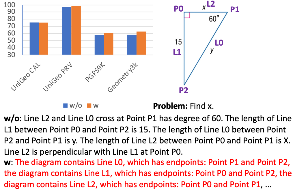
Figure 2: Top-left: the performance of the GOLD (using T5-base) with (w) and without (w/o) the geo2geo. Top-right: Geometry math problem. Bottom: Predicted diagram description with and without the geo2geo. The same text between (w) and (w/o) is omitted for space consideration, where the red text is geo2geo relations.

Table 3 shows that the GOLD model accurately captures geo2geo relation, prompting us to investigate its impact on solving geometry math problems. The bar chart in Figure 2 indicates a notable decline in model performance on the PGPS9K and Geometry3K datasets when geo2geo relations are omitted. However, this trend is less pronounced on the UniGeo datasets. This is likely because the PGPS9K and Geometry3K datasets often lack descriptions of geometric primitives in their problem texts. An example from the Geometry3K dataset, illustrated in Figure 2, demonstrates this issue: the problem text typically poses a question (e.g., "Find X") without extra information. Consequently, relying only on sym2geo relations leads to insufficient representation of essential diagram details.

5 Conclusion

In this work, we have introduced the GOLD model for automated geometry math problem-solving. GOLD uniquely converts geometry diagrams into natural language descriptions, facilitating direct integration with LLMs for problem-solving. A key feature of the GOLD model is that it separately handles symbols and geometric primitives, simplifying the process of establishing relations between symbols and geometric primitives and relations among geometric primitives themselves. Our experiments show that the GOLD model outperforms the Geoformer, the previous SOTA on the UniGeo dataset, with accuracy improvements of 12.7% and 42.1% on the UniGeo calculation and proving datasets, respectively. Additionally, compared to PGPSNet, the SOTA for the PGPS9K and Geometry3K datasets, the GOLD model shows notable accuracy improvements of 1.8% and 3.2%, respectively, showing our method’s effectiveness.

6 Limitations

While our GOLD model marks a significant advancement in solving geometry math problems, areas remain for future improvement. For example, the GOLD model has not yet reached the level of human performance in solving geometry math problems. This gap is possibly due to the limitations in fully extracting geometric relations from diagrams. While GOLD accurately identifies symbols, geometric primitives, and geo2geo relations, the extraction of sym2geo relations still requires enhancement. Moreover, this study evaluated three popular large language models (LLMs): T5-bases, Llama2-13b-chat, and CodeLlama-13b. To deepen our understanding and leverage the full potential of LLMs in solving geometry math problems, it would be beneficial to assess more LLMs. This broader evaluation could provide more comprehensive insights into optimizing LLMs for this specific task.

Appendix A Inference

During the inference stage, we employ Eq 4 and Eq 5 to map symbols $s\in\mathcal{S}$ and geometric primitives $g\in\mathcal{G}$ to corresponding vectors $\text{vec}^{s\in\mathcal{S}}$ and $\text{vec}^{g\in\mathcal{G}}$, respectively. Following this, we proceed with the inference of sym2geo and geo2geo relations.

A.1 Predict sym2geo Relation

For a text symbol $s\in\{\mathcal{S}|\text{cls}_{s}=\text{"text"}\}$, it is necessary to determine its meaning based on its text_class. To accomplish this, we assign the category of text symbol $s\in\{\mathcal{S}|\text{cls}_{s}=\text{"text"}\}$ as the one with the highest probability among the $P(\textit{text\_class}|s)$ values, as specified in Eq 6:

$$\mathit{text\_class}_{s}=\textit{argmax}P(\mathit{text\_class}|s)$$ (9)

• if $\textit{text\_class}_{s}$ is 0 (i.e., category $\mathit{0}$), it indicates that the symbol $s$ corresponds to the reference name of a point, or a line, or a circle. In this case, we assign the symbol $s$ to the geometric primitive $g$ that has the highest probability of $P(\text{rel}^{\mathit{sym2geo}}_{s\in\{\mathcal{S}|\text{cls}_{s}=\text{"text"}\},g\in\{\mathbf{P},\mathbf{L},\mathbf{C}\}}|s,g)$, where $g\in\{\mathbf{P},\mathbf{L},\mathbf{C}\}$ specifies that the geometric primitive $g$ belongs to the set of points, lines, and circles:

  $$g=\textit{argmax}P(\text{rel}^{\mathit{sym2geo}}_{s\in\{\mathcal{S}|\text{cls}_{s}=\text{"text"}\},g\in\{\mathbf{P},\mathbf{L},\mathbf{C}\}}|s,g)$$ (10)

• if $\textit{text\_class}_{s}$ is 1 (i.e., category $\mathit{1}$), it indicates that the symbol $s$ represents the degree of an angle. Since an angle consists of two lines and one point, we select the point with the highest probability $P(\text{rel}^{\mathit{sym2geo}}_{s\in\{\mathcal{S}|\text{cls}_{s}=\text{"text"}\},g\in\{\mathbf{P}\}}|s,g)$, and we select the two lines with the top two highest probabilities $P(\text{rel}^{\mathit{sym2geo}}_{s\in\{\mathcal{S}|\text{cls}_{s}=\text{"text"}\},g\in\{\mathbf{L}\}}|s,g)$. It is worth mentioning these two lines must have $geo2geo$ relations of "end-point" or "on-a-line" with the selected point.

  $$p=\textit{argmax}P(\text{rel}^{\mathit{sym2geo}}_{s\in\{\mathcal{S}|\text{cls}_{s}=\text{"text"}\},g\in\{\mathbf{P}\}}|s,g)$$ (11)

  $$l_{1},l_{2}=\textit{argmax}_{two}P(\text{rel}^{\mathit{sym2geo}}_{s\in\{\mathcal{S}|\text{cls}_{s}=\text{"text"}\},g\in\{\mathbf{L}\}}|s,g),$$

  $$\text{where }\mathit{rel}_{l_{1},p}\in\{\text{"end-point"`, "on-a-line"}\}\text{ and}$$

  $$\mathit{rel}_{l_{2},p}\in\{\text{"end-point"`, "on-a-line"}\}$$

• if $\textit{text\_class}_{s}$ is 2 (i.e., category $\mathit{2}$), it indicates that the symbol $s$ represents the length of a line. Since a line consists of two points, we select the points with the top two highest probabilities $P(\text{rel}^{\mathit{sym2geo}}_{s\in\{\mathcal{S}|\text{cls}_{s}=\text{"text"}\},g\in\{\mathbf{P}\}}|s,g)$:

  $$p_{1},p_{2}=\textit{argmax}_{two}P(\text{rel}^{\mathit{sym2geo}}_{s\in\{\mathcal{S}|\text{cls}_{s}=\text{"text"}\},g\in\{\mathbf{P}\}}|s,g)$$ (12)

• if $\textit{text\_class}_{s}$ is 3 (i.e., category $\mathit{3}$), it indicates that the symbol $s$ represents the degree of an angle on the circle. In this case, the angle is formed by the centre point of a circle and two points lying on the arc of a circle. Therefore, we first select the circle with the highest probability of $P(\text{rel}^{\mathit{sym2geo}}_{s\in\{\mathcal{S}|\text{cls}_{s}=\text{"text"}\},g\in\{\mathbf{C}\}}|s,g)$. Subsequently, we select two points with the top two highest probabilities $P(\text{rel}^{\mathit{sym2geo}}_{s\in\{\mathcal{S}|\text{cls}_{s}=\text{"text"}\},g\in\{\mathbf{P}\}}|s,g)$. Worth mentioning, these two points must be on the arc of the selected circle:

  $$c=\textit{argmax}P(\text{rel}^{\mathit{sym2geo}}_{s\in\{\mathcal{S}|\text{cls}_{s}=\text{"text"}\},g\in\{\mathbf{C}\}}|s,g)$$ (13)

  $$p_{1},p_{2}=\textit{argmax}_{two}P(\text{rel}^{\mathit{sym2geo}}_{s\in\{\mathcal{S}|\text{cls}_{s}=\text{"text"}\},g\in\{\mathbf{P}\}}|s,g)\text{,}$$

  $$\text{where }\mathit{rel}_{p_{1},c}=\mathit{rel}_{p_{2},c}=\text{"on-a-circle"}$$

For the geometric relations among geometric primitives, such as parallel. It is determined by the other2geo relation. For the other2geo relation involving other symbols, it is required that the relation holds with at least two geometric primitives. This means that there should be at least two geometric primitives with probabilities $P(\text{rel}^{\mathit{sym2geo}}_{s,g}|s,g)$ larger than a threshold $\theta$. In this case, the geometric primitives are selected based on this criterion.

$$\{g_{\text{indices}}\}=\text{sorted}(P(\text{rel}^{\mathit{sym2geo}}_{s\in\{\mathcal{S}|\text{cls}_{s}\neq\text{"text"}\},g\in{\{\mathbf{P,L,C}}}\}|s,g))>\theta$$ (14)

$${g_{\text{selected}}}=\mathcal{G}[\{g_{\text{indices}}\}]$$

where "sorted" indicates that values are sorted in descending order, and $[]$ refers to the selection from the geometric primitives group $\mathcal{G}$ according to the indices $\{g_{\text{indices}}\}$. The threshold $\theta$ is set as 0.5 experimentally.

A.2 Predict geo2geo Relation

The geo2geo relation between geometric primitives $g_{i}$ and $g_{j}$ is determined based on Eq 8, where it is assigned as the relation with the highest probability:

$$\mathit{rel}_{g_{i},g_{j}\in\mathcal{G}}=\textit{argmax}P(\text{rel}^{\mathit{geo2geo}}_{g_{i},g_{j}}|g_{i},g_{j})$$ (15)

In an ideal scenario, the OCR results would accurately provide references to the points, lines, and circles, allowing us to extract precise information about the geometric primitives. However, the open-source OCR tool we have adopted is not accurate. As a result, some primitives may lack reference names. To address this issue, we automatically label the primitives in sequential order (e.g., "P1, P2, L1, L2") if their reference names are missing.

A.3 Generate Solution Program

Once the geo2geo and sym2geo relations are constructed, we proceed to convert them into natural language descriptions $\mathcal{L}$ (See Appendix B for details). We then concatenate the natural language descriptions $\mathcal{L}$ with the problem text $\mathcal{T}$. This combined text is passed to the problem-solving module, which employs BeamSearch with a beam size of 10 to generate the solution program $\mathcal{P}$. Moreover, when using larger LLMs, such as Llama2, we add instructions in front of the concatenation of $\mathcal{L}$ and $\mathcal{T}$, which is further sent to LLMs to generate reasoning process.

Appendix B Convert Relations to Natural Language Descriptions

	Relations	Paradigm	Example
	Point	The diagram contains ${}.	The diagram contains Point A, B, C.
geo2geo	Line	The diagram contains ${}, which has endpoints: ${} and ${}, In addition, there is/are ${} on the line.	The diagram contains Line L1, which has endpoints: Point P0 and Point P1, In addition, there is/are Point P2 on the line.
	Circle	The diagram contains ${}, whose center point is ${}, which has ${} on its arc.	The diagram contains Circle M, whose center point is Point E, which has Point F, Point G on its arc.
	Degree	1. Angle ${} has degree of ${}. 2. Line ${} and Line ${} cross at Point ${} has degree of ${}.	1. Angle 1 has degree of 100. 2. Line L1 and Line L2 cross at Point C has degree of 50.
text2geo	Length	The length of Line ${} between Point ${} and Point $ is ${}.	The length of Line L3 between Point A and Point B is 10.
	Circle Degree	Line ${} and Line ${} cross at the center point ${} of Circle ${} has degree of ${}.	Line L1 and Line L2 cross at the center point C of Circle C0 has degree of 20.
	same degree	Angle ${} has the same degree with Angle ${} …	Angle 1 has the same degree with Angle 2, Angle 3.
other2geo	same length	Line ${} has the same length with Line ${} …	Line L1 has the same length with Line L2, Line L3.
	parallel	Line ${} is parallel with Line ${}…	Line a is parallel with Line b.
	perpendicular	Line ${} is perpendicular with Line ${} at Point ${}.	Line L1 is perpendicular with Line L2 at Point C.

Table 4: The defined paradigm used to convert geo2geo and sym2geo relations to natural language descriptions $\mathcal{L}$. "${}" is the placeholder. The placeholder is filled in as demonstrated in the "Example" column, and the filled content is highlighted in bold type.

Once the geo2geo relations and sym2geo relations have been established, we proceed to convert these relations into natural language descriptions denoted as $\mathcal{L}$ following the guidelines specified in Table 4.

To begin, we initiate the process by representing the existing geometric primitives in the diagram by enumerating points, lines, and circles within the description of the geo2geo relation. In detail, we sequentially enumerate all existing points, providing their reference names as described in the "Point" entry of Table 4. We describe the associated points for each line by mentioning their reference names. Additionally, we include a list of points that have "end-point" and "on-a-line" relations with the line, as specified in the "Line" entry of Table 4. Similarly, for each circle, we mention its reference name and proceed to list the points that exhibit "center-point" and "on-a-circle" relations with the circle, following the guidelines provided in the "Circle" entry of Table 4.

Next, we proceed to describe the text2geo relation within the sym2geo relation based on the predicted text_class. Here are the guidelines for each case:

• If the text_class indicates that the symbol refers to the reference name of a point (or a line, or a circle), we modify the name of the corresponding point (or line, or circle) accordingly.

• If the text_class indicates that the symbol refers to the degree of an angle, we describe it following the guidelines specified in the "Degree" entry of Table 4.

• If the text_class indicates that the symbol refers to the length of a line, we describe it according to the instructions provided in the "Length" entry of Table 4.

• If the text_class indicates that the symbol refers to the degree of an angle on the circle, we describe it based on the guidelines outlined in the "Circle Degree" entry of Table 4.

Furthermore, when dealing with the other2geo relations, we describe them based on the specific type of geometric relation as indicated in Table 4.

Appendix C Instruction Choice

Instructions serve as direct and explicit commands that clearly communicate to the model the specific task it is required to perform. For our experiments, we initially selected two distinct instruction templates for Llama2-13b-chat Touvron et al. (2023) and CodeLlama-13b Rozière et al. (2023), as detailed in Table 5. Upon experimental evaluation, it was observed that the instruction template modified from the one used to train the Llama2 model (displayed at the upper row in Table 5) demonstrated superior performance. Consequently, we opted for this template in our work.

Instruction Template	Example
[INST] You are a problem-solving bot, and now I ask you to solve a geometry problem, please answer the question and provide the correct option letter. The problem is as follows: {Problem Text} Here are the basic descriptions of the diagram: {Natural Language Descriptions} The Answer and the Reason Process are: [/INST]	[INST] You are a problem-solving bot, and now I ask you to solve a geometry problem, please answer the question and provide the correct option letter. The problem is as follows: Find the perimeter of the polygon. The Choices are: A: 20.0, B: 24.0, C: 28.0, D: 34.409, Here are the basic description of the diagram: The diagram contains Point P0, Point P1, Point P2, Point P3, Point P4, The diagram contains Line L0, which has endpoints: Point P1, Point P3, Line L1, which has endpoints: Point P1, Point P4, Line L2, which has endpoints: Point P3, Point P4, Line L3, which has endpoints: Point P0, Point P3, Line L4, which has endpoints: Point P0, Point P1, Line L5, which has endpoints: Point P0, Point P4, The length of Line L0 between Point P2 and Point P3 is 7. The length of Line L4 between Point P2 and Point P1 is 7. The length of Line L5 between Point P4 and Point P2 is 5. Line L3 between Point P0 and Point P3 has the same length with Line L4 between Point P1 and Point P0 and Line L2 between Point P3 and Point P4 and Line L1 between Point P1 and Point P4. The Answer and the Reason Process are: [/INST]
Hint: Please answer the question and provide the correct option letter, e.g., A, B, C, D, at the end {Problem Text} Here are the basic descriptions of the diagram: {Natural Language Descriptions}	Hint: Please answer the question and provide the correct option letter, e.g., A, B, C, D, at the end Find the perimeter of the polygon. The Choices are: A: 20.0, B: 24.0, C: 28.0, D: 34.409, Here are the basic descriptions of the diagram: The diagram contains Point P0, Point P1, Point P2, Point P3, Point P4, The diagram contains Line L0, which has endpoints: Point P1, Point P3, Line L1, which has endpoints: Point P1, Point P4, Line L2, which has endpoints: Point P3, Point P4, Line L3, which has endpoints: Point P0, Point P3, Line L4, which has endpoints: Point P0, Point P1, Line L5, which has endpoints: Point P0, Point P4, The length of Line L0 between Point P2 and Point P3 is 7. The length of Line L4 between Point P2 and Point P1 is 7. The length of Line L5 between Point P4 and Point P2 is 5. Line L3 between Point P0 and Point P3 has the same length with Line L4 between Point P1 and Point P0 and Line L2 between Point P3 and Point P4 and Line L1 between Point P1 and Point P4.

Table 5: Two instruction templates. The template in the upper row is modified from the instruction used to train the Llama2 model, and another one is from the Lu et al., 2023a. In the column of "Instruction Template", the "{problem Text}" is the geometry math problem text $\mathcal{T}$, and "{Natural Language Descriptions}" is the description of the diagram $\mathcal{L}$.

Appendix D Loss Function Details

The ${L}_{g2g}$ is defined as the negative log-likelihood loss, where we aim to minimize the negative log-likelihood of the ground truth relations among geometric primitives:

$$\mathit{L}_{\mathit{g2g}}=-\sum_{g_{i}\in\mathbf{P}}\sum_{g_{j}\in\mathbf{L,C}}\text{log}(P(\text{rel}^{\mathit{geo2geo}}_{g_{i},g_{j}}|g_{i},g_{j}))$$ (16)

where $g_{i}$ is a geometric primitive belonging to points, and $g_{j}$ is a geometric primitive belonging to lines and circles. The $\text{rel}^{\mathit{geo2geo}}_{g_{i},g_{j}}$ refers to the ground truth relation between $g_{i}$ and $g_{j}$.

The ${L}_{\mathit{t\_cls}}$ is defined as the negative log-likelihood loss, where we aim to minimize the negative log-likelihood of the ground truth text_class of the text symbol:

$$\mathit{L}_{\mathit{t\_cls}}\mathbin{=}\mathbin{-}\sum_{S}\text{log}(P(\textit{text\_class}_{s}|s))$$ (17)

where $\text{text\_class}_{s}$ is the ground truth $text\_class$ of the symbol $s$.

The $\mathit{L}_{\mathit{s2g}}$ is the binary cross-entropy loss:

$$\mathit{L}_{\mathit{s2g}}\mathbin{=} \mathbin{-}\sum_{s\in\mathcal{S}}\sum_{g\in\mathcal{G}}\{\mathbb{I}(s,g)\times\text{log}(P(\text{rel}^{\mathit{sym2geo}}_{s,g}|s,g))$$ (18)

$$\mathbin{+}(1\mathbin{-}\mathbb{I}(s,g))\times(1\mathbin{-}\text{log}(P(\text{rel}^{\mathit{sym2geo}}_{s,g}|s,g)\}$$

where $\mathbb{I}(s,g)$ is 1 if there is relation between symbol $s$ and geometric primitive $g$, otherwise it is 0.

The $\mathit{L}_{\mathit{prog}}$ is defined as the negative log-likelihood loss, where we aim to minimize the negative log-likelihood of the tokens of the ground truth solution programs:

$$\mathit{L}_{\mathit{prog}}\mathbin{=}\mathbin{-}\sum_{i}\text{log}(P(t_{i}|t_{<i}))$$ (19)

where $i$ is the $i$-th token in the ground truth solution program.

Appendix E Image Parsing Accuracy

Geometric Primitives or Symbols	F1 (%)
point	99.8
line	99.5
circle	99.1
symbol	97.2

Table 6: Pre-parsing performances by F1 metric.

Table 6 presents the performance of the image-parsing module, measured using the F1 metric. For geometric primitives, we employ the parsing position evaluation method, utilizing the Hough transform with a distance threshold of 15. For symbols, we use an Intersection over Union (IoU) threshold of 0.5. The results in Table 6 demonstrate that the image-parsing module delivers accurate parsing results for diagrams, providing the model with precise information.

Appendix F Relation Prediction Accuracy

Relation Type		PGPS9K Test (%)
	end-point	97.9 $\pm$ 0.3
geo2geo	on-a-line	91.3 $\pm$ 0.4
	center-point	93.6 $\pm$ 0.2
	on-a-circle	92.0 $\pm$ 0.0
	text symbol	65.2 $\pm$ 0.1
	angle	73.1 $\pm$ 0.0
sym2geo	bar	75.7 $\pm$ 0.2
	parallel	89.0 $\pm$ 0.4
	perpendicular	82.9 $\pm$ 0.0

Table 7: Relation Parsing performances by F1 metric. Both the mean and standard errors of the accuracy metrics are presented.

Table 7 displays the F1 metric for the performance of relation parsing. The results show that our GOLD model accurately predicts geo2geo relations. However, for sym2geo relations, except for the "parallel" relation, there is considerable room for improvement in the prediction performance.

Appendix G Influence of feature_embedding and spatial_embedding on Geometry Problem Solving

We conduct ablation study on feature_embedding and spatial_embedding in Table 8. To discard the use of ($\text{emb}_{\mathit{feat}}$ and $\text{emb}_{\mathit{spat}}$), we directly use feature outputs from the pre-parsing step as vectors of symbols and geometric primitives, i.e., $\mathbf{V}^{s,g}$, to construct the sym2geo and geo2geo relations. We can observe that the GOLD model without any embedding performs the worst on all test subsets. However, when either one of embeddings ($\text{emb}_{\mathit{feat}}$ or $\text{emb}_{\mathit{spat}}$) is added, the model’s performance improves. Notably, the model equipped with both embeddings achieves the best performance.

$\text{emb}_{\mathit{feat}}$	$\text{emb}_{\mathit{spat}}$	CAL	PRV	PGPS9K	Geometry3K
		66.2 $\pm$ 0.3	90.2 $\pm$ 0.2	48.2 $\pm$ 0.5	50.2 $\pm$ 0.3
		71.5 $\pm$ 0.3	93.2 $\pm$ 0.4	55.0 $\pm$ 0.1	58.1 $\pm$ 0.1
		72.8 $\pm$ 0.2	93.0 $\pm$ 0.3	56.3 $\pm$ 0.1	58.0 $\pm$ 0.2
		75.2 $\pm$ 0.3	98.5 $\pm$ 0.5	60.6 $\pm$ 0.3	62.7 $\pm$ 0.2

Table 8: Program accuracy with or without feature_embedding and spatial_embedding. The check mark () indicates that the corresponding embedding is enabled. T5-base is used as the problem-solving module for the GOLD model. Both the mean and standard errors of the accuracy metrics are presented.

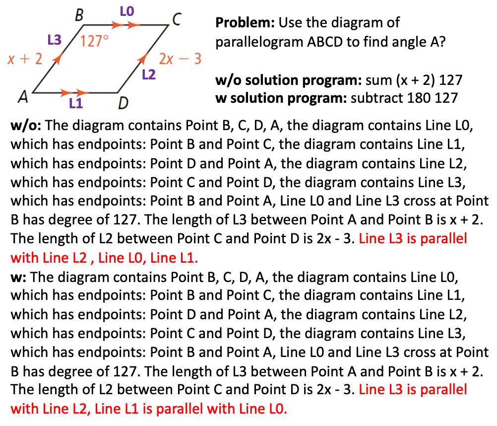
Figure 3: An example from the 111-th problem in the PGPS9K dataset. This case shows that models’ natural language descriptions and solution programs outputs with and without spatial_embedding. The purple notations in the diagram are added by us. Note that the different parts of diagram descriptions between w/o and w are coloured red.

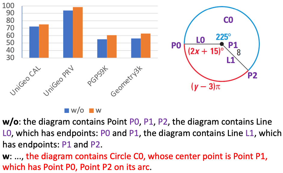
Figure 4: The top-left bar chart compares GOLD (T5-base as the problem-solving module) accuracy in solving geometry math problems, with (w) and without (w/o) the use of geo_type_embedding. The top-right diagram is from the 375th problem in the PGPS9K dataset, while the bottom part shows the predicted diagram descriptions for two different cases. Purple notations in the diagram are added for better visual comprehension. The differences between the two diagram description texts are highlighted in red. It should be noted that the same texts in the w to the w/o section are omitted, which are represented by "…".

In Figure 3, we conduct a case study on the GOLD model with and without the use of spatial_embedding. It is evident that the model without spatial_embedding incorrectly generates the "parallel" relation between lines, resulting in an erroneous solution program. This highlights the importance of spatial_embedding in capturing accurate spatial relations and improving the model’s performance.

Appendix H Importance of the geo_type_embedding

We conducted experiments to assess the impact of geo_type_embedding ($\text{emb}^{g}_{\mathit{type}}$). The top-left bar chart in Figure 4 demonstrates that the model’s performance declines when $\text{emb}^{g}_{type}$ is not utilized. Notably, the performance gaps between the model with $\text{emb}^{g}_{\mathit{type}}$ and without it are more pronounced on the PGPS9K and Geometry3K datasets compared to the UniGeo datasets. We believe this is because the problem text in the UniGeo dataset explicitly mentions the geometric primitives, providing valuable information that helps the GOLD model understand the geometric primitives more effectively. Furthermore, as shown in Figure 4, the GOLD model without $\text{emb}^{g}_{\mathit{type}}$ fails to generate accurate circle information, impeding its ability to further generate correct solution programs.

References

- Cao and Xiao (2022) Jie Cao and Jing Xiao. 2022. An augmented benchmark dataset for geometric question answering through dual parallel text encoding. In Proceedings of the 29th International Conference on Computational Linguistics, COLING 2022, Gyeongju, Republic of Korea, October 12-17, 2022, pages 1511–1520. International Committee on Computational Linguistics.
- Chen et al. (2022) Jiaqi Chen, Tong Li, Jinghui Qin, Pan Lu, Liang Lin, Chongyu Chen, and Xiaodan Liang. 2022. Unigeo: Unifying geometry logical reasoning via reformulating mathematical expression. In Proceedings of the 2022 Conference on Empirical Methods in Natural Language Processing, EMNLP 2022, Abu Dhabi, United Arab Emirates, December 7-11, 2022, pages 3313–3323. Association for Computational Linguistics.
- Chen et al. (2021) Jiaqi Chen, Jianheng Tang, Jinghui Qin, Xiaodan Liang, Lingbo Liu, Eric P. Xing, and Liang Lin. 2021. Geoqa: A geometric question answering benchmark towards multimodal numerical reasoning. In Findings of the Association for Computational Linguistics: ACL/IJCNLP 2021, Online Event, August 1-6, 2021, volume ACL/IJCNLP 2021 of Findings of ACL, pages 513–523. Association for Computational Linguistics.
- Cho et al. (2021) Jaemin Cho, Jie Lei, Hao Tan, and Mohit Bansal. 2021. Unifying vision-and-language tasks via text generation. In Proceedings of the 38th International Conference on Machine Learning, ICML 2021, 18-24 July 2021, Virtual Event, volume 139 of Proceedings of Machine Learning Research, pages 1931–1942. PMLR.
- Chou and Gao (1996a) Shang-Ching Chou and Xiao-Shan Gao. 1996a. Automated generation of readable proofs with geometric invariants i. multiple and shortest proof generation. J. Autom. Reason., 17(3):325–347.
- Chou and Gao (1996b) Shang-Ching Chou and Xiao-Shan Gao. 1996b. Automated generation of readable proofs with geometric invariants i. multiple and shortest proof generation. J. Autom. Reason., 17(3):325–347.
- Gelernter et al. (1960) Herbert L. Gelernter, J. R. Hansen, and Donald W. Loveland. 1960. Empirical explorations of the geometry theorem machine. In Papers presented at the 1960 western joint IRE-AIEE-ACM computer conference, IRE-AIEE-ACM 1960 (Western), San Francisco, California, USA, May 3-5, 1960, pages 143–149. ACM.
- He et al. (2017) Kaiming He, Georgia Gkioxari, Piotr Dollár, and Ross B. Girshick. 2017. Mask R-CNN. In IEEE International Conference on Computer Vision, ICCV 2017, Venice, Italy, October 22-29, 2017, pages 2980–2988. IEEE Computer Society.
- He et al. (2016) Kaiming He, Xiangyu Zhang, Shaoqing Ren, and Jian Sun. 2016. Deep residual learning for image recognition. In 2016 IEEE Conference on Computer Vision and Pattern Recognition, CVPR 2016, Las Vegas, NV, USA, June 27-30, 2016, pages 770–778. IEEE Computer Society.
- Hochreiter and Schmidhuber (1997) Sepp Hochreiter and Jürgen Schmidhuber. 1997. Long short-term memory. Neural Comput., 9(8):1735–1780.
- Lin et al. (2017) Tsung-Yi Lin, Piotr Dollár, Ross B. Girshick, Kaiming He, Bharath Hariharan, and Serge J. Belongie. 2017. Feature pyramid networks for object detection. In 2017 IEEE Conference on Computer Vision and Pattern Recognition, CVPR 2017, Honolulu, HI, USA, July 21-26, 2017, pages 936–944. IEEE Computer Society.
- Lu et al. (2023a) Pan Lu, Hritik Bansal, Tony Xia, Jiacheng Liu, Chunyuan Li, Hannaneh Hajishirzi, Hao Cheng, Kai-Wei Chang, Michel Galley, and Jianfeng Gao. 2023a. Mathvista: Evaluating math reasoning in visual contexts with gpt-4v, bard, and other large multimodal models. CoRR, abs/2310.02255.
- Lu et al. (2021) Pan Lu, Ran Gong, Shibiao Jiang, Liang Qiu, Siyuan Huang, Xiaodan Liang, and Song-Chun Zhu. 2021. Inter-gps: Interpretable geometry problem solving with formal language and symbolic reasoning. In Proceedings of the 59th Annual Meeting of the Association for Computational Linguistics and the 11th International Joint Conference on Natural Language Processing, ACL/IJCNLP 2021, (Volume 1: Long Papers), Virtual Event, August 1-6, 2021, pages 6774–6786. Association for Computational Linguistics.
- Lu et al. (2023b) Pan Lu, Liang Qiu, Wenhao Yu, Sean Welleck, and Kai-Wei Chang. 2023b. A survey of deep learning for mathematical reasoning. In Proceedings of the 61st Annual Meeting of the Association for Computational Linguistics (Volume 1: Long Papers), ACL 2023, Toronto, Canada, July 9-14, 2023, pages 14605–14631. Association for Computational Linguistics.
- Ning et al. (2023) Maizhen Ning, Qiu-Feng Wang, Kaizhu Huang, and Xiaowei Huang. 2023. A symbolic characters aware model for solving geometry problems. In Proceedings of the 31st ACM International Conference on Multimedia, MM 2023, Ottawa, ON, Canada, 29 October 2023- 3 November 2023, pages 7767–7775. ACM.
- Paszke et al. (2019) Adam Paszke, Sam Gross, Francisco Massa, Adam Lerer, James Bradbury, Gregory Chanan, Trevor Killeen, Zeming Lin, Natalia Gimelshein, Luca Antiga, Alban Desmaison, Andreas Köpf, Edward Z. Yang, Zachary DeVito, Martin Raison, Alykhan Tejani, Sasank Chilamkurthy, Benoit Steiner, Lu Fang, Junjie Bai, and Soumith Chintala. 2019. Pytorch: An imperative style, high-performance deep learning library. In Advances in Neural Information Processing Systems 32: Annual Conference on Neural Information Processing Systems 2019, NeurIPS 2019, December 8-14, 2019, Vancouver, BC, Canada, pages 8024–8035.
- Peng et al. (2023) Shuai Peng, Di Fu, Yijun Liang, Liangcai Gao, and Zhi Tang. 2023. Geodrl: A self-learning framework for geometry problem solving using reinforcement learning in deductive reasoning. In Findings of the Association for Computational Linguistics: ACL 2023, Toronto, Canada, July 9-14, 2023, pages 13468–13480. Association for Computational Linguistics.
- Raffel et al. (2020) Colin Raffel, Noam Shazeer, Adam Roberts, Katherine Lee, Sharan Narang, Michael Matena, Yanqi Zhou, Wei Li, and Peter J. Liu. 2020. Exploring the limits of transfer learning with a unified text-to-text transformer. J. Mach. Learn. Res., 21:140:1–140:67.
- Rozière et al. (2023) Baptiste Rozière, Jonas Gehring, Fabian Gloeckle, Sten Sootla, Itai Gat, Xiaoqing Ellen Tan, Yossi Adi, Jingyu Liu, Tal Remez, Jérémy Rapin, Artyom Kozhevnikov, Ivan Evtimov, Joanna Bitton, Manish Bhatt, Cristian Canton-Ferrer, Aaron Grattafiori, Wenhan Xiong, Alexandre Défossez, Jade Copet, Faisal Azhar, Hugo Touvron, Louis Martin, Nicolas Usunier, Thomas Scialom, and Gabriel Synnaeve. 2023. Code llama: Open foundation models for code. CoRR, abs/2308.12950.
- Sachan et al. (2017) Mrinmaya Sachan, Avinava Dubey, and Eric P. Xing. 2017. From textbooks to knowledge: A case study in harvesting axiomatic knowledge from textbooks to solve geometry problems. In Proceedings of the 2017 Conference on Empirical Methods in Natural Language Processing, EMNLP 2017, Copenhagen, Denmark, September 9-11, 2017, pages 773–784. Association for Computational Linguistics.
- Sandler et al. (2018) Mark Sandler, Andrew G. Howard, Menglong Zhu, Andrey Zhmoginov, and Liang-Chieh Chen. 2018. Mobilenetv2: Inverted residuals and linear bottlenecks. In 2018 IEEE Conference on Computer Vision and Pattern Recognition, CVPR 2018, Salt Lake City, UT, USA, June 18-22, 2018, pages 4510–4520. Computer Vision Foundation / IEEE Computer Society.
- Seo et al. (2015) Min Joon Seo, Hannaneh Hajishirzi, Ali Farhadi, Oren Etzioni, and Clint Malcolm. 2015. Solving geometry problems: Combining text and diagram interpretation. In Proceedings of the 2015 Conference on Empirical Methods in Natural Language Processing, EMNLP 2015, Lisbon, Portugal, September 17-21, 2015, pages 1466–1476. The Association for Computational Linguistics.
- Tian et al. (2022) Zhi Tian, Chunhua Shen, Hao Chen, and Tong He. 2022. FCOS: A simple and strong anchor-free object detector. IEEE Trans. Pattern Anal. Mach. Intell., 44(4):1922–1933.
- Touvron et al. (2023) Hugo Touvron, Louis Martin, Kevin Stone, Peter Albert, Amjad Almahairi, Yasmine Babaei, Nikolay Bashlykov, Soumya Batra, Prajjwal Bhargava, Shruti Bhosale, Dan Bikel, Lukas Blecher, Cristian Canton-Ferrer, Moya Chen, Guillem Cucurull, David Esiobu, Jude Fernandes, Jeremy Fu, Wenyin Fu, Brian Fuller, Cynthia Gao, Vedanuj Goswami, Naman Goyal, Anthony Hartshorn, Saghar Hosseini, Rui Hou, Hakan Inan, Marcin Kardas, Viktor Kerkez, Madian Khabsa, Isabel Kloumann, Artem Korenev, Punit Singh Koura, Marie-Anne Lachaux, Thibaut Lavril, Jenya Lee, Diana Liskovich, Yinghai Lu, Yuning Mao, Xavier Martinet, Todor Mihaylov, Pushkar Mishra, Igor Molybog, Yixin Nie, Andrew Poulton, Jeremy Reizenstein, Rashi Rungta, Kalyan Saladi, Alan Schelten, Ruan Silva, Eric Michael Smith, Ranjan Subramanian, Xiaoqing Ellen Tan, Binh Tang, Ross Taylor, Adina Williams, Jian Xiang Kuan, Puxin Xu, Zheng Yan, Iliyan Zarov, Yuchen Zhang, Angela Fan, Melanie Kambadur, Sharan Narang, Aurélien Rodriguez, Robert Stojnic, Sergey Edunov, and Thomas Scialom. 2023. Llama 2: Open foundation and fine-tuned chat models. CoRR, abs/2307.09288.
- Wen-Tsün (1986) Wu Wen-Tsün. 1986. Basic principles of mechanical theorem proving in elementary geometries. J. Autom. Reason., 2(3):221–252.
- Wolf et al. (2020) Thomas Wolf, Lysandre Debut, Victor Sanh, Julien Chaumond, Clement Delangue, Anthony Moi, Pierric Cistac, Tim Rault, Rémi Louf, Morgan Funtowicz, Joe Davison, Sam Shleifer, Patrick von Platen, Clara Ma, Yacine Jernite, Julien Plu, Canwen Xu, Teven Le Scao, Sylvain Gugger, Mariama Drame, Quentin Lhoest, and Alexander M. Rush. 2020. Transformers: State-of-the-art natural language processing. In Proceedings of the 2020 Conference on Empirical Methods in Natural Language Processing: System Demonstrations, EMNLP 2020 - Demos, Online, November 16-20, 2020, pages 38–45. Association for Computational Linguistics.
- Zhang et al. (2022) Ming-Liang Zhang, Fei Yin, Yi-Han Hao, and Cheng-Lin Liu. 2022. Plane geometry diagram parsing. In Proceedings of the Thirty-First International Joint Conference on Artificial Intelligence, IJCAI 2022, Vienna, Austria, 23-29 July 2022, pages 1636–1643. ijcai.org.
- Zhang et al. (2023) Ming-Liang Zhang, Fei Yin, and Cheng-Lin Liu. 2023. A multi-modal neural geometric solver with textual clauses parsed from diagram. In Proceedings of the Thirty-Second International Joint Conference on Artificial Intelligence, IJCAI 2023, 19th-25th August 2023, Macao, SAR, China, pages 3374–3382. ijcai.org.