Study of meson decays to and within the covariant light-front approach
Abstract
In this work, we investigate the form factors of the transitions and in the covariant light-front quark model (CLFQM), where these final states are considered as P-wave excited charmed mesons. In order to obtain the form factors for the physical transition processes, we extend these form factors from the space-like region to the time-like region. The -dependence for each transition form factor is also plotted. Then, combined with those form factors, the branching ratios of the two-body nonleptonic decays with being a light pseudoscalar (vector) meson or a charmed meson are calculated by considering the QCD radiative corrections to the hadronic matrix elements within the QCD factorization approach. Most of our predictions are comparable to the results given by other theoretical approaches and the present available data.
pacs:
13.25.Hw, 12.38.Bx, 14.40.NdI Introduction
In this work, we would like to study some of excited open-charm states, such as and in meson decays. As we know, and were first discovered by BaBar babar and CLEO cleo in 2003, respectively. The scalar charm-strange meson was observed in the invariant mass distribution of and the axial charm-strange meson was found in the invariant mass distribution of . as the partner of , called in the past, was discovered by Belle belle in the three-body decay in 2004. Another axial charm-strange meson with was first observed in the invariant mass spectrum nun in 1987.
Previous researches suggest that the masses of the resonants and are just several tens MeV below the thresholds of and , respectively. Furthermore, they are much lower than those given by the quark model quark . Some abnormal properties induce that these two states are difficult to be interpreted as conventional mesons. Therefore, many authors consider them as the molecular states guo ; cleven ; close ; guofk ; lutz ; lutz2 ; ylma , the compact tetraquark states maiani ; wangzg ; hycheng2 ; yqchen ; kim , the chiral partners of the ground state mesons bardeen ; nowak and the states of mixed with four-quark states browder ; vijande . However, if considering the coupled channel effects and the fact that there are no additional states around the quark model predicted masses, these two states can be interpreted as P-wave charm-strange mesons bracco ; lutz3 ; Hwang ; xliu ; xlchen ; jbliu ; wangzg2 ; fajfer ; song ; sfchen . As to the state, besides the low mass puzzle, where the observed mass of belle ; babar2 is bellow the predictions from the quark model about 100 MeV quark ; godfrey2 , there exists the mass hierarchy puzzle, that is the masses of and are almost equal to each other. These puzzles have triggered many studies on their inner structures: In Refs. bracco ; nielsen , the authors pointed out that the four-quark structure can explain the data measured by Belle belle and BaBar babar2 , but not for that measured by FOCUS FOCUS:2003gru . Another group authors solved these puzzles within the framework of unitarized chiral perturbation theory (UChPT) albala ; mldu ; guofk2 and considered that there exist two states in the energy region mldu2 , where the lighter one named as is the partner of the , the heavier one is a member of a different multiplet. Certainly, other authors also explained as a mixture of two and four-quark states vijande or the bound state of gamer . The axial charm-strange meson has been confirmed and studied in the meson decays by BaBar babar3 , Belle belle2 and LHCb lhcb . Its measurements of mass and width are consistent with the theoretical expectations as a charm-strange meson with . As we know that the QCD Lagrangian is invariant under the heavy flavor and spin rotation in the heavy quark limit. For the heavy mesons, the heavy quark spin can decouple from the other degrees of freedom. Then and the total angular momentum of the light quark become good quantum numbers. It is natural to label and by the quantum numbers with being the total (orbital) angular momentum of the light quark, that is and , denoted as and , respectively. Since the heavy quark symmetry is not exact, the two states and can mix with each other through the following formula belle3
| (1) |
While the states and are expected to be a mixture of states and with and , respectively,
| (2) |
Combining Eq. (1) and Eq. (2), one can find that
| (3) |
where zhw .
Using the manifestly covariant of the Bethe-Salpeter (BS) approach Salpeter:1951sz ; Salpeter:1952ib , Jaus, Choi, Ji and Cheng et al. Jaus:1999zv ; Choi:1998nf ; Cheng:1997au put forward the CLFQM around 2000. This approach provides a systematic way to explore the zero-mode effects, which are just cancelled by involving the spurious contributions being proportional to the lightlike four-vector , at the same time the covariance of the matrix elements being restored Jaus:1999zv . Up to now the CLFQM has been used extensively to study the weak and radiative decays, as well as the features of some exotic hadrons Cheng:2003sm ; w.wang ; x.wang ; w.wang2 ; ke ; Li:2010bb ; Sun1 ; Sun2 ; Sun3 . In this work, we will employ the CLFQM to evaluate the transition form factors, then calculate the branching ratios of the relevant decays. In our calculations these hadrons are regarded as ordinary meson states. Compared with the future experimental measurements, our predictions are helpful to clarify the inner structures of these four hadrons.
The arrangement of this paper is as follows: In Section II, an introduction to the CLFQM and the expressions for the form factors of the transitions are presented. Then the branching ratios of the meson decays with one of these considered P-wave excited charm sates involved are calculated under the QCD factorization approach, where the vertex corrections and the hard spectator-scattering corrections are considered. In Section III, the numerical results of the transition form factors and their -dependence are presented. Then, combined with the transition form factors, the branching ratios of the decays with being a light pseudoscalar (vector) meson or a charmed meson are calculated. In addition, detailed numerical analysis and discussion, including comparisons with the data and other model calculations, are carried out. The conclusions are presented in the final part.
II Formalism
II.1 The Covariant Light-Front Quark Model
Under the covariant light-front quark model, the light-front coordinates of a momentum are defined as with and . If the momenta of the quark and antiquark with mass and in the incoming (outgoing) meson are denoted as and , respectively, the momentum of the incoming (outgoing) meson with mass can be written as . Here, we use the same notation as those in Refs. Jaus:1999zv ; Cheng:2003sm and refers to for meson decays. These momenta can be related each other through the internal variables
| (4) |
with . Using these internal variables, we can define some quantities for the incoming meson which will be used in the following calculations:
| (5) |
where the kinetic invariant mass of the incoming meson can be expressed as the energies of the quark and the antiquark . It is similar to the case of the outgoing meson.
The form factors of the transitions 222It is similar for the transition . From now on, we will use and to represent and , respectively, for simplicity. and 333We will use and to represent and , respectively. The form factors of the transitions and can be obtained from those of the transitions and through Eq. (3). induced by the vector and aixal-vector currents are defined as
| (6) | |||||
| (7) | |||||
| (8) |
In calculations, the Bauer-Stech-Wirbel (BSW) bsw transition form factors are more frequently used and defined by
| (9) | |||||
| (10) | |||||
| (11) |
where , and the convention is adopted.
To smear the singularity at in Eq. (10), the relations are required, and
| (12) |
These two kinds of form factors are related to each other via
| (13) | |||||
| (14) | |||||
| (15) |
The light-front wave functions (LFWFs) are needed in the form factor calculations. Although the LFWFs can be derived from solving the relativistic Schrdinger equation theoretically, it is difficult to obtained their exact solutions in many cases. Consequently, we will use the phenomenological Gaussian-type wave functions in this work,
| (16) |
where the parameter describes the momentum distribution and is approximately of order . It can be usually determined by the decay constants through the following analytic expressions Jaus:1999zv ; Cheng:2003sm ,
| (17) | |||||
| (18) | |||||
| (19) |
where and represent the constituent quarks of the states and . The decay constants can be obtained through experimental measurements for the purely leptonic decays or theorical calculations. The explicit forms of are given by Cheng:2003sm
| (20) | |||||
| (21) |
II.2 Form factors
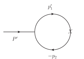
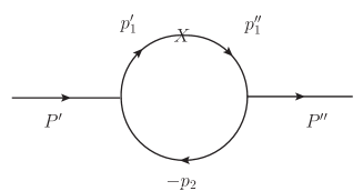
For the general transitions with being a scalar or axial-vector meson Cheng:2003sm , the decay amplitude at the lowest order is
| (22) |
where arise from the quark propagators. For our considered transitions and , the traces and can be directly obtained by using the Lorentz contraction as follows
| (23) | |||||
| (24) | |||||
| (25) | |||||
To calculate the amplitudes for the transition form factors, we need the Feynman rules for the meson-quark-antiquark vertices (), which are listed as
| (26) | |||||
| (27) | |||||
| (28) |
In practice, we employ the light-front decomposition of the Feynman loop momentum and integrate out the minus component using the contour method. Then additional spurious contributions being proportional to the light-like four-vector will appear. While they can be eliminated by including the zero-mode contributions in a proper way. If the covariant vertex functions are not exhibit singularity during integration, the transition amplitudes will capture the singularities in the antiquark propagators. The specific rules for the integration have been derived in Refs. Jaus:1999zv ; Cheng:2003sm , and the relevant ones are summarized in Appendix A. The integration then leads to
| (29) |
where
| (30) |
with and . The explicit forms of have been given in Eq. (20) and Eq. (21).
Using Eq. (20)-Eq. (30) and taking the integration rules given in Refs. Jaus:1999zv ; Cheng:2003sm , the form factors and , , , can be obtained directly, which are listed in Appendix C.
II.3 Vertex Corrections and The Hard Spectator Function
Within the framework of QCD factorization BBNS , the short-distance nonfactorizable corrections including the vertex corrections and hard spectator interactions are considered. The modifications of the Wilson coefficients from the vertex corrections are given as
| (31) |
with being the meson emitted from the weak vertex. The vertex functions are written as BBNS
| (32) |
where and are the decay constant and the twist-2 meson distribution amplitude of the meson , respectively. The hard kernel is
| (33) | |||||
The modifications of the Wilson coefficients from the hard spectator-scattering corrections arising from a hard gluon exchange between the emitted meson and the spectator quark are written as
| (34) |
where the hard spectator functions are defined as Cheng:2007st
| (35) |
with and . and are the twist-2 and twist-3 LCDAs of the meson . The definations of and can be found in Ref. Cheng:2007st .
III Numerical results and discussions
III.1 Transition Form Factors
. Mass(GeV)
| Decay constants(GeV) | ||
|---|---|---|
The input parameters, such as the masses of the initial and final mesons, the decay constants, are listed in Table 1. The decay constants of the axial mesons and can be obtained from and through the mixing between and
| (36) |
Using these decay constants and the masses of the constituent quarks and mesons given in Table 1, we can obtain the values of the shape parameters for our considered mesons, which are listed in Table 2.
| 0.317 | 0.37 | |||
|---|---|---|---|---|
It is noticed that all the computations are conducted within the reference frame, where the form factors can only be obtained at spacelike momentum transfers . It is necessary to know the form factors in the timelike region for the physical decay processes. Here, we utilize the following double-pole approximation to parameterize the form factors in the spacelike region and then extend to the timelike region,
| (37) |
where represents the initial meson mass and denotes the different form factors. The values of and can be obtained by performing a 3-parameter fit to the form factors in the range , which are collected in Tables 3 and 5. The uncertainties arise from the decay constants of the initial meson and the final state mesons.
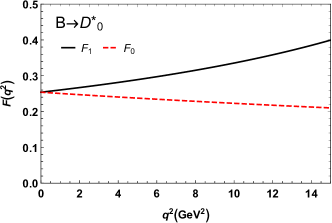
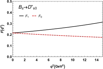
In Table 3, we list the form factors of the transitions . One can find that the form factors of the transitions are much smaller. This conclusion is also supported by other works, for example, the form factor of the transtion was obtained as 0.24 and 0.18 within the CLFQM Cheng:2003sm and the 2nd version of the Isgur-Scora-Grinstein-Wise (ISGW2) approach Cheng:2003id , respectively. Furthermore, our result for the form factor of the transtion is consistent with 0.20 gvien in the ISGW2 model Cheng:2003id , while smaller than 0.40 given by the QCD sum rules (QCDSR) approach T.M. . As to the form factors of the transitions , they have been searched by many appoaches, such as the Melikhov-Stech (MS) model Melikhov:2000yu , the relaticistic quark model (RQM) Kramer2 , the BSW model bsw ; Kramer:1992xr , the Bethe-Salpeter (BS) equation Chen:2011ut , the QCDSR Blasi:1993fi and the light cone sum rules (LSCR) approach Ball:1998tj . Cosidering the need for the latter branching ratio calcuations, we also give them in Table 4 with other theoretical results for comparison. Obviously, our predictions are consistent well with these theoretical results.
| a | b | |||
|---|---|---|---|---|
| Transitions | References | |||||
|---|---|---|---|---|---|---|
| This work | ||||||
| Cheng:2003sm | ||||||
| Melikhov:2000yu | ||||||
| bsw | ||||||
| This work | ||||||
| Kramer2 | ||||||
| Kramer:1992xr | ||||||
| Chen:2011ut | ||||||
| Blasi:1993fi | ||||||
| This work | ||||||
| Cheng:2003sm | ||||||
| Ball:1998tj | ||||||
| Melikhov:2000yu | ||||||
| bsw | ||||||
| This work | ||||||
| Cheng:2003sm | ||||||
| Ball:1998tj | ||||||
| Melikhov:2000yu | ||||||
| bsw |
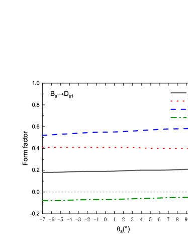
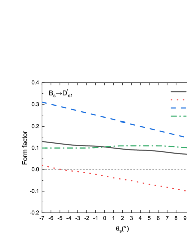
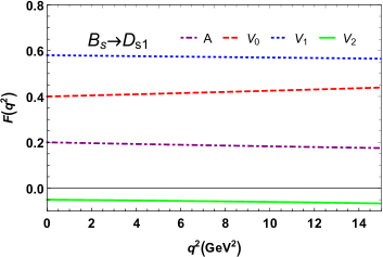
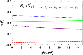
In order to determine the physical form factors of the transitions , we need to know the mixing angle between and shown in Eq. (3). Here we take , which was determined from the quark potential model Cheng:2003id . The results are listed in Table 5, where the uncertainties are from the decay constants of and the final states (, ). In Figure 2, we check the dependence of the form factors of the transitions on the mixing angle . We find that the form factor of the transition () is (not) sensitive to the mixing angle. It can be used to explain why the branching ratios of the decays associated with the transition () are (not) sensitive to the mixing angle, which will be discussed in the latter.
| a | b | |||
|---|---|---|---|---|
In Figure 3, we plot the -dependence of the form factors of the transitions . There exists the similar -dependence of the form factors between the transitions and . It is consistent with our expectation. While it is very different in magnitude between the corresponding form factors for the transitions and .
III.2 Branching ratios
In addition to the parameters listed in Table 1, other inputs, such as the meson lifetime , the Wilson coefficients and the CabibboKobayashi-Maskawa (CKM) matrix elements, are listed as pdg22 ; Beneke:2001ev
| (38) | |||||
| (39) | |||||
| (40) | |||||
| (41) |
Firstly, we consider the branching ratios of the decays with being a light pseudoscalar (vector) meson or a charmed meson , which can be calculated through the formula
| (42) |
where the decay width for each channel is given as following
| (43) | |||||
| (44) |
where refers to () and the subscript . can be obtained by replacing with , in Eq. (44). There exists similar expressions for the cases with replaced by in the upper decays. While for the charged decays with being , the corresponding decay widths should be written as
| (45) | |||||
| (46) | |||||
Secondly, the decay widths of the decays are defined as
| (47) | |||||
| (48) | |||||
| (49) | |||||
where represents a vector meson, such as , and the summation of the three polarizations for the decays are performed. The three-momentum is defined as
| (50) |
and the three polarization amplitudes and are given as
| (51) |
with and , . As to the decay widths of the decays and , they can be obtained from Eqs. (48) and (49) with some simple replacements, respectively. Using the upper listed input parameters and the formulas given in Eq. (42)-Eq. (51), one can calculate the branching ratios for the considered decays shown in Tables 6-13.
| LO | VC | HSSC | NLO | Other predictions | Refs. | |
|---|---|---|---|---|---|---|
| PQCD Wang:2018fai | ||||||
| CLFQM Cheng:2003sm | ||||||
| ISGW2 Cheng:2003id | ||||||
| ISGW Katoch:1995hr | ||||||
| PQCD Wang:2018fai | ||||||
| ISGW2 Cheng:2003id | ||||||
| ISGW Katoch:1995hr | ||||||
| PQCD Wang:2018fai | ||||||
| PQCD Wang:2018fai | ||||||
From Table 6, one can find that the branching ratios of the decays and are sensitive to the vertex corrections. These two channels are contributed by two kinds of Feynman diagrams, one is associated with the transition accompanied by the emission of a light pseudoscalar meson (), the other is associated with the transition accompanied by the scalar meson emission. We can find that the former gives the dominant contribution. The other two decay channels and only receive one kind of Feynman diagram contribution to the their branching ratios, which is associated with the transition accompanied by a light pseudoscalar meson () emission. In any case, the contributions from the vertex corrections and the hard spectator-scatterings are destructive with each other. In view of the large uncertainty from the decay constant as mentioned before, two decay constant values are used in our calculations, which are shown in Table 6. For each decay, the upper line is the result corresponding to GeV, and the lower is the result corresponding to GeV. We can find that the branching ratios are sensitive to the decay constant . Our predictions are consistent with other theoretical calculations, such as the PQCD approach Wang:2018fai , the ISGW quark model Cheng:2003id ; Katoch:1995hr . Certainly, the branching ratio of the decay was also calculated using the CLFQM in previous Cheng:2003sm , which is agreement with our result.
| This work | PQCD Wang:2018fai | Data | |
|---|---|---|---|
| Belle belle | |||
| BaBar babar2 | |||
| LHCb LHCb:2016lxy | |||
| Belle Belle:2006wbx | |||
| LHCb LHCb:2015klp | |||
| LHCb LHCb:2015klp | |||
| LHCb LHCb:2015eqv | |||
| LHCb LHCb:2015tsv | |||
The branching ratio of the quasi-two-body decay can be obtained from the corresponding two body decay under the narrow width approximation , where refers to a light pseudoscalar meson (). Assuming the state decays essentially into D, we have from the Clebsch-Gordan coefficients. The branching ratios of these quasi-two-body decays are collected in Table 7, where the PQCD results and the data are also listed for comparison. One can find that if taken the bigger decay constant GeV, the branching fraction for the decay can agree with the data from Belle belle , BaBar babar2 and LHCb LHCb:2016lxy within errors. While for the decay , if taken the smaller decay constant GeV, our prediction can explain the LHCb measurement LHCb:2015tsv . For the other two quasi-two-body decays, the predictions for their branching ratios are much larger than the present data. Similar situation exists for the comparison between the PQCD results and the measurements. Another divergence is that our results for the charged (neutral) channels by using the bigger (smaller) decay constant GeV can be consistent well with the PQCD results. Further experimental and theoretical researches are needed to clarify these divergences and puzzles.
| LO | VC | HSSC | NLO | ISGW2 Cheng:2003id | ISGW Katoch:1995hr | |
|---|---|---|---|---|---|---|
If replaced the light pseudoscalar mesons in the final states with the vector meson and the charmed meson , the branching ratios for the conrresponding decay channels are listed in Table 8. One can find that our predictions by using the bigger decay constant GeV are consistent with those given in the ISGW model, it is because that the form factor of the transition at maximum momentum transfer obtained in the CLFQM with GeV is about 0.30, which is almost equal to the value calculated in the ISGW model Katoch:1995hr , while much larger than 0.18 given in the ISGW2 model Cheng:2003id . The differences between the ISGW and ISGW2 models are mainly from the -dependence of the form factor. About twteen years ago, Chua Chua:2003ac studied the decay in the CLFQM approach and obtained its branching fraction about , which is consistent with our result by taking GeV.
| LO | ||||
|---|---|---|---|---|
| VC | ||||
| HSSC | ||||
| NLO | ||||
| PQCD Zhang:2019pax | ||||
| LSCR Li:2009wq | ||||
| RQM Kramer2 | ||||
| NRQM Albertus:2014bfa | ||||
| ISGW2 Cheng:2003id |
Taking as a meson, we calclate the branching ratios of the decays with being a pseudoscalar meson () or a vector meson in the CLFQM, which are listed in Tables 9, 10 and 11. From Table 9, one can find that our predictions for the decays are consistent well with those calculated in the LCSR Li:2009wq and the PQCD approach Zhang:2019pax within errors, while (much) smaller than those given by the RQM Kramer2 and the nonrelativistic quark model (NRQM) Albertus:2014bfa . Especially, for the pure annihilation decay , its branching fraction reaches up to predicted by the NRQM Albertus:2014bfa , which seems too large compared to other theoretical results. These divergences can be clarified by the future LHCb and Super KEKB experiments. The branching ratios of the decays were also calculated in the ISGW2 model Cheng:2003id , which are smaller than our results. It is because of the difference from the form factor of the transition and its -dependence. It is similar for the decays .
| LO | ||||
|---|---|---|---|---|
| VC | ||||
| HSSC | ||||
| NLO | ||||
| PQCD Zhang:2021bcr | ||||
| FH Faessler:2007cu | ||||
| TM Liu:2022dmm | ||||
| Data pdg22 |
In Table 10, all the predictions from the different theories, including the PQCD approach Zhang:2021bcr , the factorization hypothesis (FH) Faessler:2007cu and the triangle mechanism (TM) Liu:2022dmm , show that the branching ratios of the charged decay are slightly larger than those of the corresponding neutral decays . It is just contrary to the case of the data pdg22 . Certainly, there still exist large errors in the experimental results, especially for the branching ratios of the decays with the vector meson involved. We expect more accurate measurements in the future LHCb and Super KEKB experiments. Theoretically, the decays and have the same CKM matrix elements and Wilson coefficients for the factorizable emission amplitudes, which provide the dominant contributions to their branching ratios. Furthermore, there exist similar transition form factors for isospin symmetry among these channels. So these four decays should have similar branching ratios. From Table 11, one can find that the branching ratios of the decays are consistent with those given in the PQCD approach Zhang:2019pax and the RQM Kramer2 , while much smaller than those obtained within the LCSR Li:2009wq . Further experimental and theoretical researches are needed to clarify these divergences. For the decays , their branching ratios are much smaller than those of other four channels mainly because of the smaller CKM matrix element compared with , that is to say there exists a suppressed factor for the decays compared to other four channels.
| LO | VC | HSSC | NLO | PQCD Zhang:2021bcr | RQM Kramer2 | LSCR Li:2009wq | |
|---|---|---|---|---|---|---|---|
In the quark model the axial-vector mesons exist in two types of spectroscopic states, and . In some cases the physical particles are the mixture of these two types of states. For example, and are considered as the mixture of and for the mass difference of the strange and light quarks. Similarly, the charm-strange mesons and are usually written as the mixture of the states and , which are given in Eq. (3). The quark potential model determined the mixing angle Cheng:2003id . So we use to calculate the branching ratios of the decays with and being the pseudoscalar mesons () and the vector mesons , respectivley, which are listed in Table 12 with the results given in the RQM, the NRQM and the ISGW2 models Kramer2 ; Albertus:2014bfa ; Cheng:2003id for comparison. The following points can be found
-
•
It is interesting that our predictions for the decays are consistent well with the results obtained in the RQM Kramer2 and NRQM Albertus:2014bfa models, while those for most of the channels are about times smaller than the RQM calculations. Certainly, the decays and have been researched by using the ISGW2 model Cheng:2003id about twenty years ago. We argue that the mixing formula between and used in Ref. Cheng:2003id is incorrect, which induced are larger than . It is just contrary with other theoretical predictions. That is to say the values of the branching raitos and should be exchanged with each other under the correct mixing formula shown in Eq. (3). Since many of these decays have large branching ratios, which lie in the range , we expect that the LHCb and Super KEKB experiments can clarify the differences between these results in the future.
-
•
The branching ratios of the CKM-favored decays and , which are associated with the CKM matrix elements and , respectively, are much larger than those of the CKM-suppressed channels and , which are associated with the CKM matrix elements and , respectively. It shows a clear hierarchical relationship for the branching raitos of these color-favored decay modes,
(52) Table 12: The branching ratios () of the decays . The labels LO, VC, HSSC, NLO and the error sources are the same with those given in Table 6. The results given in the RQM, the NRQM and the ISGW2 models are also listed for comparison. LO VC HSSC NLO RQM Kramer2 NRQM Albertus:2014bfa ISGW2 Cheng:2003id -
•
Our predictions for the branching ratios of the decays are at least one order larger than those of the corresponding decays . This is because that the related form factor is much larger than that of . There exists the similar situation between the branching ratios of the decays and , where is at the emission position in the Feynman diagrams.
-
•
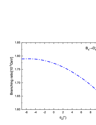
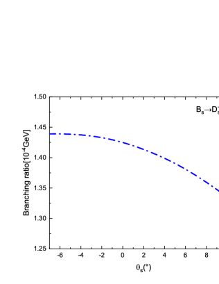
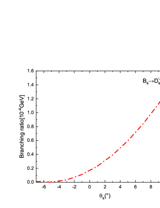
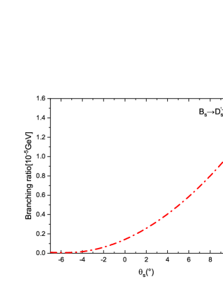
In view of the mixing angle uncertainty, we check the dependence of the branching ratios of the decays on the mixing angle , which are shown in Figure 4. One can find that the branching ratios of the decays are very sensitive to the mixing angle, while those of the decays show an insensitive dependence on . Furthermore, the changing trends for the branching ratios of these two kinds of decays are just opposite.
| LO | VC | HSSC | NLO | ISGW2 Cheng:2003id | ISGW Katoch:1996hr | FH Faessler:2007cu | TM Liu:2022dmm | Data pdg22 ; ijmp | |
|---|---|---|---|---|---|---|---|---|---|
In Table 13, we present our predictions for the branching ratios of the decays , which are associated with the transition, accompanied by the emission. When the emission meson is , our results for the decays and are larger than those given by the ISGW(2) Cheng:2003id ; Katoch:1996hr and the FH Faessler:2007cu by a factor of to . While for other two decays and , our predictions are consistent well with the theoretical and experimental results within errors except for those given in Ref. Liu:2022dmm , where the triangle mechanism was used by considering as a molecular state. When the emission meson is , the branching ratios of the decays and are at least one order smaller than those of the decays and . It is because of the much smaller decay constant compared to . Such character has been verified by the data shown in Table 13.
III.3 SUMMARY
Firstly, we studied the form factors of the transitions and in the covariant light-front quark model (CLFQM). One can find that these form factors are (much) smaller than those of the transitions . Certainly, because of the mixing between and , the determination of the form factors for the transitions are more difficult. Secondly, using the amplitudes combined via the form factors, we calculated the branching ratios of the nonleptonic decays with these four charmed mesons involved. Furthermore, the QCD radiative corrections to the hadronic matrix elements within the framework of QCD factorization were included. From the numerical results, we found the following points
-
1.
The small form factors of the transitions are related to the small decay constants . Unfortunately, there exit large uncertainties in these two decay constants. Combined with the data, our predictions for the branching ratios of the decays with involved are helpful to probe the inner structures of these two states. Most of the decays with P(V) being a light pseudoscalar (vector) meson or a charmed meson are not sensitive to the QCD radiative corrections including the vertex corrections and the hard spectator-scattering, except for the decays , where two kinds of Feynman diagrams contribute to the branching ratios. Our predictions for the branching ratios of the quasi-two-body decays and can explain the data by taking appropriate decay constant value for , while for the decays and , their branching ratios are much larger than the LHCb measurements. There exist the similar cases for the PQCD calculations compared with the data.
-
2.
We checked the dependence of the branching ratios of the decays on the mixing angle and found that the branching ratios of the decays are very sensitive to the mixing angle, while those of the decays show an insensitive dependence on . The changing trends of the branching ratios between these two kinds of decays are just opposite. Furthermore, the branching ratios of the decays are at least one order larger than those of the decays . It is because of the larger form factor compared to . Such a feature is similar to the decays , where the is at the emission position in the Feynman diagrams, that is to say the branching ratios of the decays are at least one order larger than those of the decays . It is because of the larger decay constant compared to . This character has been verified by the experimental measurements.
-
3.
Our predictions are helpful to clarify the different assumptions about the inner structures of these four charmed hadrons by comparing with the future data.
Acknowledgment
This work is partly supported by the National Natural Science Foundation of China under Grant No. 11347030, by the Program of Science and Technology Innovation Talents in Universities of Henan Province 14HASTIT037.
Appendix A Some specific rules under the intergration
When preforming the integraion, we need to include the zero-mode contributions. It amounts to performing the integration in a proper way in the CLFQM. Specificlly we use the following rules given in Refs. Jaus:1999zv ; Cheng:2003sm
| (53) | |||||
| (54) | |||||
| (55) |
| (56) | |||||
| (57) |
Appendix B EXPRESSIONS OF FORM FACTORS
| (58) | |||||
| (59) | |||||
| (60) | |||||
| (61) | |||||
| (62) | |||||
| (63) | |||||
with .
References
- (1) B. Aubert et al. [BaBar], Phys. Rev. Lett. 90, 242001 (2003) [arXiv:hep-ex/0304021].
- (2) D. Besson et al. [CLEO], Phys. Rev. D 68, 032002 (2003) [Erratum: Phys. Rev. D 75, 119908 (2007)] [arXiv:hep-ex/0305100].
- (3) K. Abe, et al. [Belle], Phys. Rev. D 69 112002 (2004) [arXiv:hep-ex/0307021].
- (4) A. E. Asratian, et al., Z. Phys. C 40 483 (1988).
- (5) S. Godfrey and N. Isgur, Phys. Rev. D 32, 189 (1985).
- (6) Z. X. Xie, G. Q. Feng and X. H. Guo, Phys. Rev. D 81, 036014 (2010).
- (7) M. Cleven, H. W. Griehammer, F. K. Guo, C. Hanhart and U. G. Meiner, Eur. Phys. J. A 50, 149 (2014) [arXiv:1405.2242 [hep-ph]].
- (8) F. K. Guo, P. N. Shen, H. C. Chiang, R. G. Ping, and B. S. Zou, Phys. Lett. B 641, 278 (2006) [arXiv:hep-ph/0603072].
- (9) T. Barnes, F. E. Close and H. J. Lipkin, Phys. Rev. D 68, 054006 (2003) [arXiv:hep-ph/0305025].
- (10) E. E. Kolomeitsev and M. F. M. Lutz, Phys. Lett. B 582, 39 (2004) [arXiv:hep-ph/0307133].
- (11) J. Hofmann and M. F. M. Lutz, Nucl. Phys. A 733, 142 (2004) [arXiv:hep-ph/0308263].
- (12) C. J. Xiao, D. Y. Chen and Y. L. Ma, Phys. Rev. D 93, 094011 (2016) [arXiv:1601.06399 [hep-ph]].
- (13) L. Maiani, F. Piccinini, A. D. Polosa, and V. Riquer, Phys. Rev. D 71, 014028 (2005) [arXiv:hep-ph/0412098].
- (14) Z. G. Wang and S. L. Wan, Nucl. Phys. A 778, 22 (2006) [arXiv:hep-ph/0602080].
- (15) H. Y. Cheng and W. S. Hou, Phys. Lett. B 566, 193 (2003) [arXiv:hep-ph/0305038].
- (16) Y. Q. Chen and X. Q. Li, Phys. Rev. Lett. 93, 232001 (2004) [arXiv:hep-ph/0407062].
- (17) H. Kim and Y. Oh, Phys. Rev. D 72, 074012 (2005) [arXiv:hep-ph/0508251].
- (18) W. A. Bardeen, E. J. Eichten, and C. T. Hill, Phys. Rev. D 68, 054024 (2003) [arXiv:hep-ph/0305049].
- (19) M. A. Nowak, M. Rho, and I. Zahed, Acta Phys. Polon. B 35, 2377 (2004) [arXiv:hep-ph/0307102].
- (20) T. E. Browder, S. Pakvasa, and A. A. Petrov, Phys. Lett. B 578, 365 (2004) [arXiv:hep-ph/0307054].
- (21) J. Vijande, F. Fernandez, and A. Valcarce, Phys. Rev. D 73, 034002 (2006) [arXiv:hep-ph/0601143].
- (22) M. E. Bracco, A. Lozea, R. D. Matheus, F. S. Navarra and M. Nielsen, Phys. Lett. B 624, 217 (2005) [arXiv:hep-ph/0503137].
- (23) M. F. M. Lutz and M. Soyeur, Prog. Part. Nucl. Phys. 61, 155 (2008).
- (24) D. S. Hwang and D. W. Kim, Phys. Lett. B 601, 137 (2004) [arXiv:hep-ph/0408154].
- (25) X. Liu, Y. M. Yu, S. M. Zhao and X. Q. Li, Eur. Phys. J. C 47, 445 (2006) [arXiv:hep-ph/0601017].
- (26) J. Lu, X. L. Chen, W. Z. Deng and S. L. Zhu, Phys. Rev. D 73, 054012 (2006) [arXiv:hep-ph/0602167].
- (27) J. B. Liu and M. Z. Yang, JHEP 1407, 106 (2014) [arXiv:1307.4636 [hep-ph]].
- (28) Z. G. Wang, Phys. Rev. D 75, 034013 (2007) [arXiv:hep-ph/0612225].
- (29) S. Fajfer and A. P. Brdnik, Phys. Rev. D 92 , 074047 (2015) [arXiv:1506.02716 [hep-ph]].
- (30) Q. T. Song, D. Y. Chen, X. Liu and T. Matsuki, Phys. Rev. D 91, 054031 (2015) [arXiv:1501.03575 [hep-ph]].
- (31) S. F. Chen, J. Liu, H. Q. Zhou, and D. Y. Chen, Eur. Phys. J. C 80, 290 (2020) [arXiv:2003.07988 [hep-ph]].
- (32) B. Aubert, et al. [BaBar] , Phys. Rev. D 79 112004 (2009) [arXiv:0901.1291 [hep-ex]].
- (33) S. Godfrey and R. Kokoski, Phys. Rev. D 43 1679 (1991).
- (34) M. Nielsen, R. D. Matheus, F. S. Navarra and M. E. Bracco, Nucl. Phys. B 161 193 (2006).
- (35) J. M. Link et al. [FOCUS], Phys. Lett. B 586, 11 (2004) [arXiv:hep-ex/0312060].
- (36) M. Albaladejo, P. Ferniäandez-Soler, F. K. Guo, and J. Nieves, Phys. Lett. B 767, 465 (2017) [arXiv:1610.06727 [hep-ph]].
- (37) M. L. Du, M. Albaladejo, P. Ferniäandez-Soler, F. K. Guo, C. Hanhart, U. G. Meiner, J. Nieves, and D. L. Yao, Phys. Rev. D 98, 094018 (2018) [arXiv:1712.07957 [hep-ph]].
- (38) F. K. Guo, C. Hanhart, U. G. Meiner, Q. Wang, Q. Zhao, and B. S. Zou, Rev. Mod. Phys. 90, 015004 (2018) [arXiv:1705.00141 [hep-ph]].
- (39) M. L. Du, F. K. Guo, C. Hanhart, B. Kubis and U. G. Meiner, Phys. Rev. Lett. 126, 192001 (2021) [arXiv:2012.04599 [hep-ph]].
- (40) D. Gamermann, E. Oset, D. Strottman and M. J. Vicente Vacas, Phys. Rev. D 76, 074016 (2007) [arXiv:hep-ph/0612179]
- (41) B. Aubert, et al. [BaBar], Phys. Rev. D 77, 011102 (2008) [arXiv:0708.1565 [hep-ex]].
- (42) T. Aushev, et al. [Belle], Phys. Rev. D 83, 051102 (2011) [arXiv:1102.0935 [hep-ex]].
- (43) R. Aaij, et al. [LHCb], Phys. Rev. D 86, 112005 (2012) [arXiv:1211.1541 [hep-ex]].
- (44) V. Balagura,et al. [Belle], Phys. Rev. D 77, 032001 (2008) [arXiv:0709.4184 [hep-ex]].
- (45) Z. H. Wang, Y. Zhang, T. h. Wang, Y. Jiang, Q. Li and G. L. Wang, Chin. Phys. C 42, 123101 (2018) [arXiv:1803.06822 [hep-ph]].
- (46) E. E. Salpeter and H. A. Bethe, Phys. Rev. 84, 1232 (1951).
- (47) E. E. Salpeter, Phys. Rev. 87, 328 (1952).
- (48) W. Jaus, Phys. Rev. D 60, 054026 (1999).
- (49) H. M. Choi and C. R. Ji, Phys. Rev. D 58, 071901 (1998) [arXiv:hep-ph/9805438].
- (50) H. Y. Cheng, C. Y. Cheung, C. W. Hwang and W. M. Zhang, Phys. Rev. D 57 5598 (1998) [arXiv:hep-ph/9709412].
- (51) H. Y. Cheng, C. K. Chua and C. W. Hwang, Phys. Rev. D 69, 074025 (2004) [arXiv:hep-ph/0310359].
- (52) W. Wang, Y. L. Shen and C. D. Lu, Phys. Rev. D 79, 054012 (2009) [arXiv:0811.3748 [hep-ph]].
- (53) X. X. Wang, W. Wang and C. D. Lu, Phys. Rev. D 79, 114018 (2009) [arXiv:0901.1934 [hep-ph]].
- (54) W. Wang, Y. L. Shen and C. D. Lu, Eur. Phys. J. C 51, 841 (2007) [arXiv:0704.2493 [hep-ph]].
- (55) H. W. Ke, T. Liu and X. Q. Li, Phys. Rev. D 89, 017501 (2014) [arXiv:1307.5925 [hep-ph]].
- (56) G. Li, F. l. Shao and W. Wang, Phys. Rev. D 82, 094031 (2010) [arXiv:1008.3696 [hep-ph]].
- (57) Z. Q. Zhang, Z. J. Sun, Y. C. Zhao, Y. Y. Yang and Z. Y. Zhang, Eur. Phys. J. C 83, 477 (2023) [arXiv:2301.11107 [hep-ph]].
- (58) Z. J. Sun, S. Y. Wang, Z. Q. Zhang, Y. Y. Yang and Z. Y. Zhang, Eur. Phys. J. C 83, 945 (2023) [arXiv:2308.03114 [hep-ph]].
- (59) Z. J. Sun, Z. Q. Zhang, Y. Y. Yang and H. Yang, Eur. Phys. J. C 84, 65 (2024) [arXiv:2311.04431 [hep-ph]].
- (60) M. Wirbel, B. Stech and M. Bauer, Z. Phys. C 29, 637 (1985).
- (61) M. Beneke, G. Buchalla, M. Neubert, and C. T. Sachrajda, Phys. Rev. Lett. 83, 1914 (1999) [arXiv:hep-ph/9905312].
- (62) H. Y. Cheng, C. K. Chua and K. C. Yang, Phys. Rev. D 77, 014034 (2008) [arXiv:0705.3079 [hep-ph]].
- (63) M. Beneke and M. Neubert, Nucl. Phys. B 675, 333 (2003) [arXiv:hep-ph/0308039].
- (64) R. L. Workman et al. [Particle Data Group], Review of Particle Physics. PTEP 2022, 083C01 (2022).
- (65) D. Becirevic, P. Boucaud, J. P. Leroy, V. Lubicz, G. Martinelli, F. Mescia and F. Rapuano, Phys. Rev. D 60, 074501 (1999) [arXiv:hep-lat/9811003].
- (66) H. Y. Cheng, Phys. Rev. D 68, 094005 (2003) [arXiv:hep-ph/0307168].
- (67) R. H. Li and C. D. Lu, Phys. Rev. D 80, 014005 (2009) [arXiv:0905.3259 [hep-ph]].
- (68) T. M. Aliev and M. Savci, Phys. Rev. D 73, 114010 (2006) [arXiv:hep-ph/0604002].
- (69) D. Melikhov and B. Stech, Phys. Rev. D 62, 014006 (2000) [arXiv:hep-ph/0001113].
- (70) R. N. Faustov and V. O. Galkin, Phys. Rev. D 87, 034033 (2013) [arXiv:1212.3167 [hep-ph]].
- (71) G. Kramer and W. F. Palmer, Phys. Rev. D 46, 3197 (1992).
- (72) X. J. Chen, H. F. Fu, C. S. Kim and G. L. Wang, J. Phys. G 39, 045002 (2012) [arXiv:1106.3003 [hep-ph]].
- (73) P. Blasi, P. Colangelo, G. Nardulli and N. Paver, Phys. Rev. D 49, 238 (1994) [arXiv:hep-ph/9307290].
- (74) P. Ball, JHEP 09, 005 (1998) [arXiv:hep-ph/9802394].
- (75) M. Beneke, G. Buchalla, M. Neubert and C. T. Sachrajda, Nucl. Phys. B 606, 245 (2001) [arXiv:hep-ph/0104110].
- (76) W. F. Wang, Phys. Lett. B 788, 468 (2019) [arXiv:1809.02943 [hep-ph]].
- (77) A. C. Katoch and R. C. Verma, Int. J. Mod. Phys. A 11, 129 (1996).
- (78) R. Aaij et al. [LHCb], Phys. Rev. D 94, 072001 (2016) [arXiv:1608.01289 [hep-ex]].
- (79) A. Kuzmin et al. [Belle], Phys. Rev. D 76, 012006 (2007) [arXiv:hep-ex/0611054].
- (80) R. Aaij et al. [LHCb], Phys. Rev. D 92, 032002 (2015) [arXiv:1505.01710 [hep-ex]].
- (81) R. Aaij et al. [LHCb], Phys. Rev. D 91, 092002 (2015) [erratum: Phys. Rev. D 93, 119901 (2016)] [arXiv:1503.02995 [hep-ex]].
- (82) R. Aaij et al. [LHCb], Phys. Rev. D 92, 012012 (2015) [arXiv:1505.01505 [hep-ex]].
- (83) C. K. Chua, J. Korean Phys. Soc. 45, S256 (2004) [arXiv:hep-ph/0312075].
- (84) Z. Q. Zhang, H. Guo, N. Wang and H. T. Jia, Phys. Rev. D 99, 073002 (2019) [arXiv:1903.03990 [hep-ph]].
- (85) C. Albertus, Phys. Rev. D 89, 065042 (2014) [arXiv:1401.1791 [hep-ph]].
- (86) Z. Q. Zhang, M. G. Wang, Y. C. Zhao, Z. L. Guan and N. Wang, Phys. Rev. D 103, 116030 (2021) [arXiv:2105.02688 [hep-ph]].
- (87) A. Faessler, T. Gutsche, S. Kovalenko and V. E. Lyubovitskij, Phys. Rev. D 76, 014003 (2007) [arXiv:0705.0892 [hep-ph]].
- (88) M. Z. Liu, X. Z. Ling, L. S. Geng, E. Wang and J. J. Xie, Phys. Rev. D 106, 114011 (2022) [arXiv:2209.01103 [hep-ph]].
- (89) J. Segovia, D. R. Entem, F. Fernandez, E. Hernandez, Int. J. Mod. Phys. E 22, 1330026 (2013) [arXiv:1309.6926 [hep-ph]].
- (90) A. C. Katoch and R. C. Verma, J. Phys. G 22, 1765 (1996).