Reconfigurable nonreciprocal heat transport with natural bulk materials

Abstract

Non-reciprocity is increasingly scrutinised in contemporary physics and engineering, especially in the realm of heat transport. This concept opens up novel avenues for directional heat transport and thermal regulation. Nonetheless, the development of non-reciprocal thermal metamaterials confronts three primary challenges: a constrained operational temperature range and structural scale, considerable energy dissipation, and the limitation of non-reciprocal effects due to external parameters that are not freely adjustable. To surmount these hurdles, we propose a reconfigurable approach to non-reciprocal heat transport. The design features a simple asymmetrical structure, with a flat panel made of natural, evenly-distributed material, positioned vertically on one side of a central horizontal board. We employ natural convection on the vertical plate to facilitate non-reciprocal heat transport. The reconfigurability of non-reciprocal heat transport is achieved by adjusting the number of vertical plates and their thermal conductivity. Theoretical computations of the rectification ratio are employed to quantify and forecast the non-reciprocal effect, corroborated by simulations and empirical studies. Beyond the quantity of plates and thermal conductivity, we also establish correlations between the rectification ratio and various parameters, including the vertical plates’ positioning and height, ambient temperature, and the temperature differential between heat sources. Control over multiple parameters can efficaciously widen the scope of non-reciprocal control and streamline experimental procedures. Furthermore, our research exclusively utilises the natural convection of air for non-reciprocal heat transport, obviating the need for supplementary energy sources and markedly enhancing energy efficiency. This study represents a significant stride in the domain of irreversible thermal management and offers pivotal insights for non-reciprocal research in other diffusion systems.

I Introduction

The study of non-reciprocity in classical systems plays a pivotal role in numerous areas of modern physics and engineering, such as thermal energy managementJuAM23 , signal transmissionDaiLSA12 , mechanical waveguidesNasNRM20 , and biomedicineHokSA96 . Reciprocity means that in a system, the response behaves the same in the reverse path as in the forward path. According to the Onsager-Casimir theorem, a medium that satisfies the assumptions of linearity, time invariance, and microscopic reversibility is a reciprocal medium. Non-reciprocity can be achieved if one or more assumptions of the Onsager-Casimir theorem are violatedCalPRAP18 , meaning the system’s response is no longer reversible along the original path. Non-reciprocity in wave systems is often achieved by breaking time-reversal symmetry, including the application of magneto-optic materials BiNP21 , nonlinear effectsFanSCI12 ; BenPRL13 ; CaoPRL17 , time modulationSouNP17 ; GuoLSA19 ; ZhangAM19 , and the addition of active elements with specific directionalityFleSCI14 ; YangPRL15 ; MaNAT18 . The emergence of metamaterialsDongJAP04 ; HuangPRE03 ; YePA0818 ; LiuPO13 ; HuangAPL05 ; QiuJPCB15 has opened up new avenues for achieving non-reciprocity, particularly in the realms of acoustic and optical metamaterialsKadNRP19 , as well as in the domains of active metamaterialsPopNC14 ; BraNC18 ; FruNAT21 , and mechanical metamaterialsCouNAT17 ; SchNP20 . Corresponding functional devices such as isolatorsFangNP17 , circulatorsEstNP14 ; BeNC17 , topological insulatorsNasNRM20 , rectifierLiangNM10 , diodesBaeAM13 , and sensorsLauNC18 have been developed. Diffusion, another fundamental mechanism of energy and mass transport, is therefore crucial in the study of non-reciprocity in diffusion systems. Wave systems are time-reversal symmetric, while diffusive movements like charge transport and thermal conduction follow time-reversal asymmetric principlesCamNC20 . Thus, transporting methods of achieving non-reciprocity in wave systems to diffusion systems requires careful handling.

Thermal transportJinAM23 ; XuCPL20 ; JinIJHMT20 ; ZhuAIP15 ; XuIJHMT21 ; XuPRAP20 ; XuPRAP19 ; YangAPL17 ; DaiJAP18 ; GaoJPC07 ; XuPRE18 , a typical example of a diffusive processYangRMP23 ; ZhangNRP23 ; XuES20 ; ShenAPL16 ; YangES19 , exhibits non-reciprocity as the spatial asymmetry of heat transfer between two spatial points. Non-reciprocal thermal transport is significant for applications in energy collection or effective heat dissipation. There are mainly four methods to achieve non-reciprocal thermal transport, as shown in Figure 1a. Firstly, introducing nonlinear effects is one of the most common methodsLiPRL15 , with thermal diodes being the most direct applicationWehAPL17 ; KobAPL09 . Secondly, the introduction of convectionXuPRL22-1 ; JinPNAS23 . Thermal conduction is irreversible on a macroscopic scale but obeys time-reversal symmetry at the microscopic level, making it reversible at the microscopic scale. Therefore, akin to the non-reciprocity induced by circulating fluids in acousticsFleSCI14 , thermal convection can similarly produce non-reciprocity in thermal conductionXuAPL21 . This leads to the development of two-port global thermal reciprocity and three-port thermal circulatorsLiPRB21 ; JuAM23-1 . Thirdly, equivalent convection generated by spatiotemporal modulation can also break the inherent spatial symmetry of thermal conductionTorPRL18 ; LiNC22 ; XuPRL22-2 . Fourthly, non-reciprocal thermal transport due to active metamaterials or asymmetric structures designSuPRAP23 ; XuPNAS23 ; XuNSR23 ; HeAM23 . Despite many achievements in non-reciprocal thermal transport, three challenges remain in the practical application of non-reciprocal thermal metamaterials. First, non-reciprocal thermal transport devices designed with nonlinear effects are limited to specific temperature ranges and scales related to the phase transition temperatures of shape memory alloys. Second, nonreciprocity caused by convection or other external field biases can lead to high energy losses. Third, whether it’s convection or spatiotemporal modulation, the effect of non-reciprocity is limited by external parameters and is difficult or even impossible to adjust once the structure is set.

In response to these challenges, we use asymmetric structures and natural convection to achieve reconfigurable non-reciprocal thermal transport, as shown in Figure 1. The entire structure is made of natural bulk materials, and the asymmetric structure is achieved by applying vertical plates off-center to a horizontal base plate. Considering the natural convection of air on the vertical plates, we can achieve reconfigurable non-reciprocity by adjusting the number $N$ of vertical plates and the thermal conductivity $\kappa$ of the materials. The theoretical calculation of the rectification ratio quantifies the non-reciprocal effect, deriving strict mathematical relationships between various parameters and the rectification ratio, validated by experiments and simulations. The non-reciprocal heat transport effect is also modulated by the the position $a$ of the vertical plates, the height $L$ of vertical plates, the ambient temperature $T_{amb}$, and temperature difference $\delta T=|T_{1}-T_{2}|$ between hot and cold sources. Multiple parameter controls expand the boundaries of non-reciprocity control, simplifying experimental operations. The sole use of natural convection significantly reduces energy consumption and improves energy utilization, opening new paths for non-reciprocal thermal control.

II Principle of reconfigurable non-reciprocal heat transport

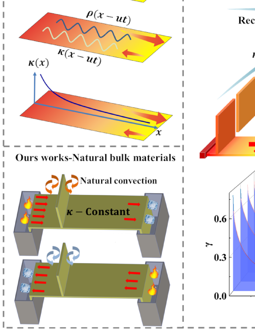
Figure 1: Principles of reconfigurable non-reciprocal heat transport. A comparison is made between previous schemes and our proposed scheme in (a). In previous works, achieving non-reciprocal heat transport requires the use of complex artificial structure metamaterials. There are four main methods: nonlinearity, convection introduction, spatiotemporal regulation, and asymmetric structures. We have simplified the preparation difficulty and achieved non-reciprocal heat transport by applying natural convection on an asymmetric structure made of natural homogeneous materials. (b) The number $N$ of vertical plates and material thermal conductivity $\kappa$ can be adjusted to achieve non-reciprocal reconfigurability. (c) Non-reciprocal structures are modulated by multiple parameters and have a wide modulation range.

We analyze the thermal field distribution of the whole struture to quantify the non-reciprocal effects and predict parameter-dependent variations. The structure is divided into four sections: three on the base plate (areas I, II, III) and the vertical plate (area IV), as shown in Figure 2a. Area II can be regarded as the staggered area between the base plate and the vertical plate. We apply heat and cold sources to the base plate’s ends and consider linear heat conduction. Apart from heat transport from the base plate, there is also thermal exchange with the air on the vertical board. The vertical plate, acting as an extension of the base plate, has a temperature distribution following an exponential function (refer to Appendix A). Given the vertical plate’s thinness compared to the base plate’s length, it’s assumed that the temperature at the interface of Regions II and IV is even. The temperature distribution on the z-axis is the primary focus in Region IV. Write out the temperature distribution forms for four regions, considering the continuity of temperature and heat flow at the contact surfaces between regions to list the boundary conditions, from which the temperature distribution of the entire structure can be derived. The derivation details are provided in Appendix A. By considering the geometric parameters and material coefficients as constants, we can map the temperature distribution on both the vertical plates and base (shown in Figures 2b-c). This reveals a difference in the temperature profiles in the forward and backward directions of the base plate, demonstrating non-reciprocal heat transport. The vertical plate also shows a higher overall temperature in the forward direction compared to the backward direction. The disparity in natural convection-driven heat dissipation $q_{conv}=hA_{s}(T_{IV}-T_{amb})$ between the vertical plate and the air in different directions further confirms this non-reciprocity. Here $T_{IV}$ is the temperature of the vertical plate, $T_{amb}$ is the ambient temperature, $h$ is the natural convection coefficient and $A_{s}$ is the contact area between the vertical plate and the air. We substitute the parameters used in the theory into the simulation, and the simulated temperature line diagram coincide with the theoretical line diagram, indicating the correctness of the theory.

To more intuitively demonstrate the non-reciprocal effect, we analyze the heat flow distribution in the base plate along the $x$ direction, as depicted in Figure 2b. Under natural convection, the heat flow values in Areas I and III show significant differences between the forward and backward directions. Notably, a substantial change in heat flow occurs when passing through Area II, due to a portion of the heat diverting to Area IV. Unlike previous studies where heat flow is typically continuous, our study observes abrupt changes in heat flow, with constant values in Areas I and III. This distinction prompts a separate calculation of inflow and outflow heat values. We introduce the rectification ratios $\gamma_{1}$ and $\gamma_{2}$, defined as:

$$\begin{array}[]{c}\gamma_{1}=\frac{|q_{FI}-q_{BIII}|}{|q_{FI}+q_{BIII}|},\\ \gamma_{2}=\frac{|q_{FIII}-q_{BI}|}{|q_{FIII}+q_{BI}|}.\end{array}$$ (1)

Here, $\gamma_{1}$ represents the discrepancy in heat flow inflow between forward and backward directions, dependent solely on the forward inflow ($q_{FI}=|-\kappa A\nabla T_{FI}(x)|$) and backward inflow ($q_{BIII}=|-\kappa A\nabla T_{BIII}(x)|$), where $\kappa$ refers to the thermal conductivity of the material, and $A$ is the cross-sectional area of the base plate in the x direction. The subscripts ’F’ and ’B’ denote ’Forward’ and ’Backward’, respectively. Similarly, $\gamma_{2}$ quantifies the difference in outflow heat flow values, involving the forward outflow ($q_{FIII}=|-\kappa A\nabla T_{FIII}(x)|$) and backward outflow ($q_{BI}=|-\kappa A\nabla T_{BI}(x)|$). The maximum value of either rectification ratio is 1, indicating exclusive inflow or outflow in the forward direction with none in the backward direction.

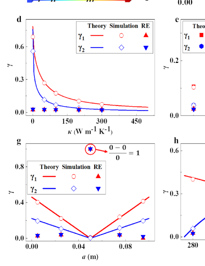
Figure 2: Theory and simulation results for reconfigurable non-reciprocal heat transport. (a) Structural diagram. The entire structure is divided into 4 areas, the vertical plate Area IV, and the base plate is divided into Areas I, II, and III. (b) Temperature distribution at the centerline of the base plate and total heat flow distribution in the base plate. (c) Temperature distribution profiles along the centerlines of the vertical plate. (d)-(i) Rectification ratio ($\gamma_{1}$ and $\gamma_{2}$, representing inflow and outflow respectively) changes with material thermal conductivity $\kappa$, number $N$ of vertical plates, height $L$ of vertical plates , position $a$ of vertical plates, ambient temperature $T_{amb}$, and temperature difference $\delta T=|T_{1}-T_{2}|$ between hot and cold sources. RE represents the relative error between theoretical value and simulated value.

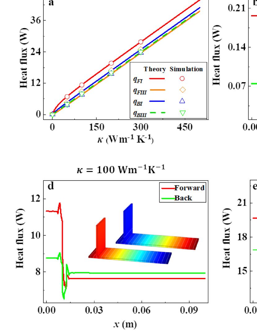
Figure A2: (a) Inflow and outflow heat flow values as a function of thermal conductivity $\kappa$. (b)-(f) Display simulated temperature and heat flow diagrams for thermal conductivities of 0.5 $\rm Wm^{-1}K^{-1}$, 50 $\rm Wm^{-1}K^{-1}$, 100 $\rm Wm^{-1}K^{-1}$, 200 $\rm Wm^{-1}K^{-1}$, and 300 $\rm Wm^{-1}K^{-1}$, respectively.

Our study demonstrates that asymmetric structural design combined with natural convection can lead to non-reciprocal heat transport. This effect can be modulated through various parameters, notably the thermal conductivity ($\kappa$) of the material. By varying $\kappa$, we can significantly influence the heat transport rectification ratio. Figure 2d illustrates how rectification ratio changes with thermal conductivity. We observe that as $\kappa$ increases, both the inflow and outflow rectification ratios decrease, eventually approaching an extreme value. This trend is due to the inverse relationship between thermal conductivity and temperature variation across the vertical plate during forward and backward heat transport; lower $\kappa$ results in higher temperature during forward transport and lower temperature during backward transport, enhancing the natural convection difference and, hence, a larger rectification ratio. For instance, at $\kappa=0.01~{}\rm Wm^{-1}K^{-1}$, the values of $\gamma_{1}$ and $\gamma_{2}$ are 0.79 and 0.76, respectively, indicating a pronounced non-reciprocal effect. We conduct simulations with five different thermal conductivity values – 0.5, 50, 100, 200, and 300 $\rm Wm^{-1}K^{-1}$ – and analyzed the inflow and outflow heat flow values for each (detailed results available in the Appendix B, Figure A2). The calculated rectification ratios for these simulations, depicted in Figure 2d, align with the theoretical predictions, further validating our theoretical approach.

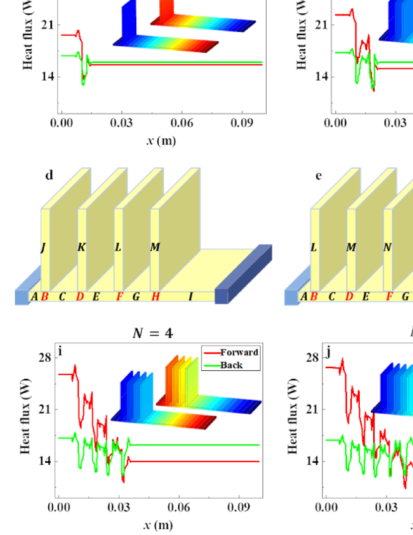
Figure A3: (a)-(e) Structural diagrams with 1, 2, 3, 4, and 5 vertical plates, respectively. For clearer visual representation, the thickness and spacing of the vertical plates are exaggerated; however, in reality, all vertical plates are positioned off-center. (f)-(j) Display simulated temperature and heat flow diagrams. (k) Heat flow values as a function of the number of vertical plates.

The rectification ratio can also be fine-tuned by varying the number $N$ of vertical plates in the structure. In our theoretical model, each plate is treated uniformly. Adding a vertical plate introduces six additional variables due to the creation of three new regions in the structure. We derive the thermal field distribution for the entire structure by solving these simultaneous boundary conditions, with further details available in Appendix C. By inputting consistent parameters into our simulations, we can visualize the heat flow of the entire structure and calculate the rectification ratio (simulation results presented in Figure A3 of the Appendix C). The impact of varying plate numbers on rectification ratios is illustrated in Figure 2e, using a thermal conductivity of $\kappa=200~{}\rm Wm^{-1}K^{-1}$. The theoretical and simulation results closely align, with an average numerical difference of 3%., which is considered highly accurate. We observe that both inflow and outflow rectification ratios increase with the number of plates, indicating that each additional plate enhances the difference in natural convection between the forward and backward directions. However, this trend varies with thermal conductivity. For instance, at $\kappa=2.1~{}\rm Wm^{-1}K^{-1}$, the rectification ratio initially increases with the plate number, reaching a peak at two plates, and then decreases (as detailed in Appendix D). This variation occurs because, low thermal conductivity leads to a lower temperature on the vertical plates near the center compared to the surrounding environment during forward heat transport. At this time, the natural convection of all vertical plates to the outside will be reduced, thus reducing the rectification ratio. Consequently, the relationship between rectification ratio and plate number is dependent on thermal conductivity. Achieving the maximum rectification ratio requires a balanced consideration of both the number of plates and their thermal conductivity.

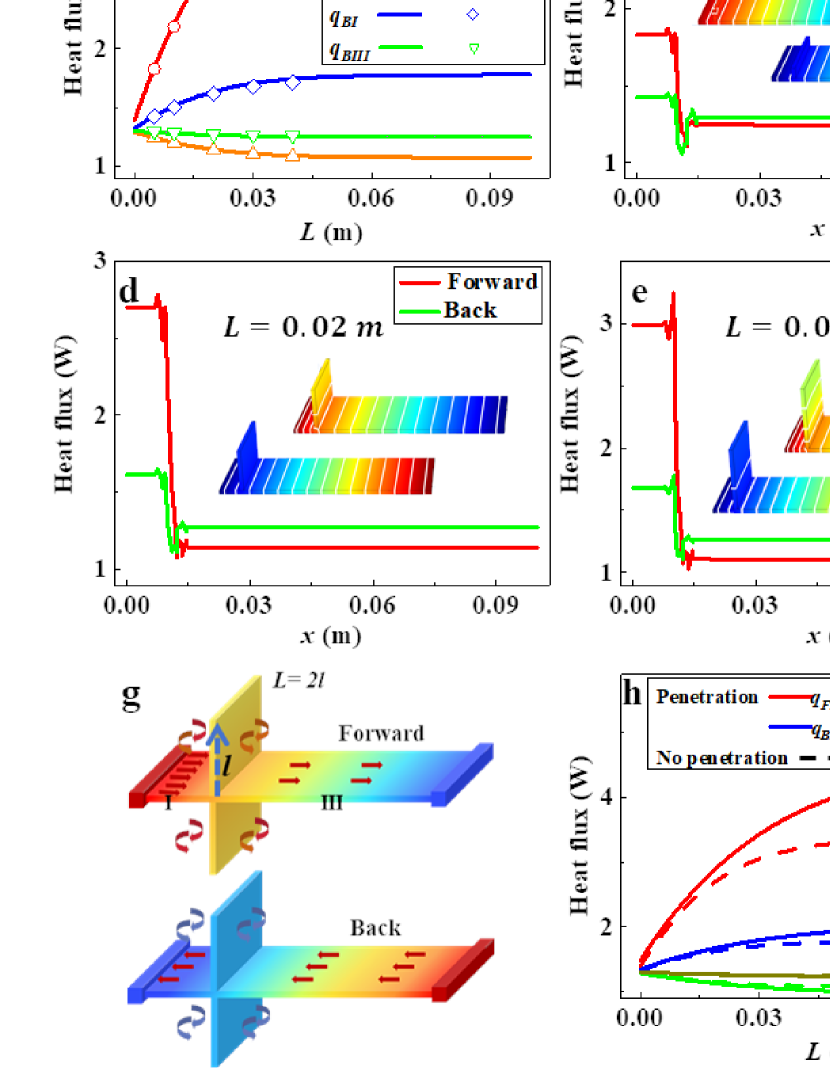
Figure A5: (a) Illustrate how both heat flow value vary with vertical plate height $L$, juxtaposing theoretical results (solid lines) with simulation data (points). (b) to (f) Feature simulated temperature profiles and heat flow diagrams corresponding to the data points in panel (a), with vertical plate heights of 0.005 m, 0.01 m, 0.02 m, 0.03 m, and 0.04 m. (g) Illustrates a vertical plate intersecting the base plate, with $l$ denoting the height of the vertical plate above the base. The total vertical plate length is $L=2l$. (h) and (i) Display variations in heat flow and rectification ratio with changes in vertical plate height, contrasting penetration (solid line) with non-penetration (dotted line).

Several other parameters also influence the rectification ratio, including the height of the vertical plate ($L$), its position ($a$), ambient temperature ($T_{amb}$), and the temperature difference ($\delta_{T}$) between the cold and hot sources. We fix the thermal conductivity $\kappa=16.3~{}\rm Wm^{-1}K^{-1}$ and the number $N=1$ of vertical plates. The rectification ratio results are shown in Figures 2f-i, and the simulation details are provided in Appendix E-H. Increasing $L$ expands the area for natural convection, thus enhancing the rectification ratio by amplifying the difference in natural convection between forward and backward directions. However, this effect plateaus at a certain height, as heat transport along the vertical plate eventually reaches equilibrium with the ambient temperature. Beyond this height, additional plate length contributes minimally to the rectification ratio. Alternatively, extending vertical plates through the base plate can further increase natural convection and thus the rectification ratio (see Figures A5g-i of the Appendix E). The vertical plate’s position also impacts the rectification ratio. Positions closer to the center yield lower ratios due to reduced asymmetry. Perfectly centered plates lead to symmetrical, reciprocal heat transport with zero theoretical and simulated rectification ratios. The ambient temperature $T_{amb}$ inversely influences the inflow and outflow rectification ratios—lowering the former and raising the latter. When $T_{amb}$ matches the average temperature of the cold and hot sources, the rectification ratios $\gamma_{1}$ and $\gamma_{2}$ become equal. Additionally, maintaining a constant temperature at one source ($T_{1}$) while increasing the temperature at the other ($T_{2}$), thus raising $\delta T=|T_{1}-T_{2}|$, reduces the outflow rectification ratio. The inflow rectification ratio decreases first and then increases with $\delta T$. When the overall temperature of the system is lower than $T_{amb}$, the air heats the vertical plate, and as the increase in $\delta T$ weakens the heating effect, the inflow rectification ratio decreases. However, when the system temperature is higher than $T_{amb}$, the air cools the vertical plate, and as the increase in $\delta T$ enhances the heating effect, the inflow rectification ratio increases. This asymmetric structure is not only simple and broadly applicable but also offers extensive parameter adjustability, reducing operational complexity. Importantly, it achieves non-reciprocity solely through natural convection, without the need for additional power configurations. This approach minimizes energy waste and enhances energy efficiency.

III Numerical and experimental verification of non-reciprocal heat transport

We use simulations and experiments to verify the reconfigurable non-reciprocity of this asymmetric metamaterial under natural convection. We focus on the parameters most influential to the rectification ratio: thermal conductivity and the number of vertical plates. In order to maximize the natural convection of the vertical panels and enhance the structural stability, the vertical plates penetrate the base plates. In our analysis, increasing the number of vertical plates in materials with high thermal conductivity enhances the rectification ratio. We select a design with five vertically oriented boards penetrating the base board.

We test samples made from four different materials: copper ($\kappa=386.4~{}\rm Wm^{-1}K^{-1}$), aluminum alloy ($\kappa=209~{}\rm Wm^{-1}K^{-1}$), brass ($\kappa=116.7~{}\rm Wm^{-1}K^{-1}$), and stainless steel ($\kappa=16.3~{}\rm Wm^{-1}K^{-1}$), as depicted in Figure 3a. In the simulations, all base plate surfaces, except for the cold and heat sources in the x-direction, are treated as thermally insulated. The vertical plates are subjected to natural convection at an ambient temperature of $T_{amb}=305$ K and a convection coefficient of $h=8~{}\rm Wm^{-1}K^{-1}$. The temperatures of the heat and cold sources are set at 330 K and 290 K, respectively. Figure 3b display the simulated temperature distributions and thermal streamline diagrams for these samples. Both forward and backward heat flows in all samples exhibit distinct non-reciprocal behavior. The heat flow values in Regions I and III are analyzed and compared with theoretical predictions in Figure 3c, using the same parameters for theory and simulation. While heat flow values increase with thermal conductivity, and the theoretical and simulated values closely align, it is less evident how the discrepancy between forward and back heat flow ($q_{FI}$ and $q_{BIII}$ for inflow, $q_{FIII}$ and $q_{BI}$ for outflow) varies with thermal conductivity. Thus, we calculate the rectification ratio using Equation 1, presented in Figure 3d. It is observed that both inflow and outflow rectification ratios decrease as thermal conductivity increases, with copper exhibiting the smallest ratio and stainless steel the largest.

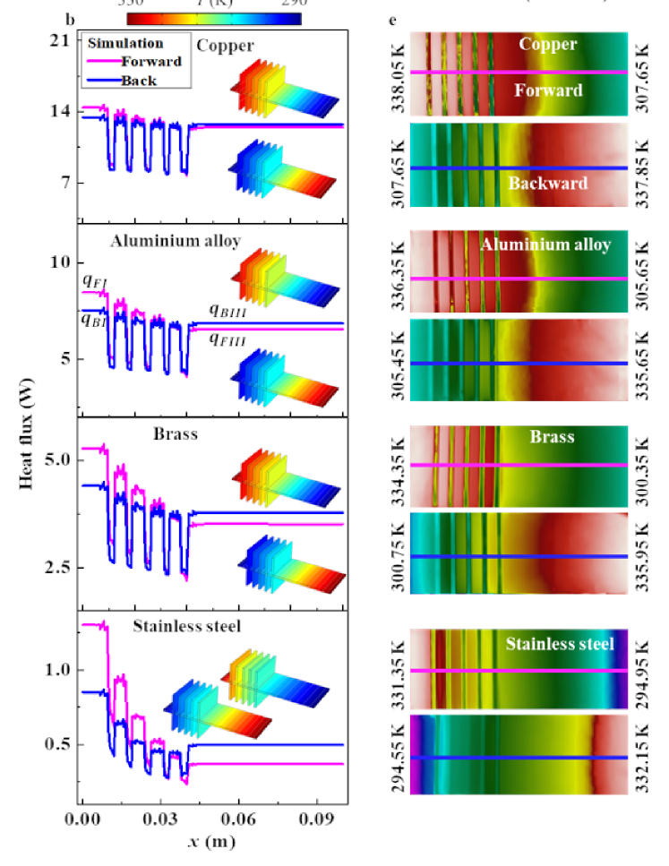
Figure 3: Theoretical, simulation and experimental results of non-reciprocal heat transport configurations with different thermal conductivity. (a) Structural diagrams of four material configuration. (b) Simulation outcomes for four different materials: copper ($\kappa=386.4~{}\rm Wm^{-1}K^{-1}$), aluminum alloy ($\kappa=209~{}\rm Wm^{-1}K^{-1}$), brass ($\kappa=116.7~{}\rm Wm^{-1}K^{-1}$), and stainless steel ($\kappa=16.3~{}\rm Wm^{-1}K^{-1}$). (c) Analysis of how heat flow values change with thermal conductivity, covering forward inflow (FI), forward outflow (FIII), back inflow (BIII), and back outflow (BI). These values are derived from the simulations shown in Figures 3b. (d) The variation of inflow rectification ratio ($\gamma_{1}$) and outflow rectification ratio ($\gamma_{2}$) in relation to thermal conductivity. (e) Experimental results demonstrating the temperature field distribution for each of the four materials. (f) A comparative analysis of the temperature distribution along the base plate’s centerline between experimental results and simulation data. The parameters employed in the simulations are consistent with those used in the experiments.

Further, we create eight experimental samples, two from each material. For each material, we place two samples simultaneously in opposite directions within the cold and heat sources. We capture overhead images to record the surface temperature distribution of the base plate, with results displayed in Figure 3e, following the order of copper, aluminum alloy, brass, and stainless steel. During the experiments, completely isolating the base plate’s natural convection proves challenging. However, whether or not the base plate has natural convection does not impact our non-reciprocal conclusions, as detailed in Appendix I. The primary difference lies in whether the base plate heat flow distribution remains linear. Consequently, we conduct experiments with the entire structure exposed to air. We simulate each sample using the same temperatures for the hot and cold sources as in the experiments. The entire structure’s surface is set for natural convection in the simulations, with a convection coefficient of $h=8~{}\rm Wm^{-2}K^{-1}$, a value determined through comparative analysis of simulations and experiments. The ambient temperature is set at the actual experimental value, $T_{amb}=301.4$ K.

We compare the temperature distribution along the centerline of the base plate with simulation results, as shown in Figure 3f. There is a good overlap between the experimental and simulated line graphs. The significant temperature fluctuations seen in the experimental data are attributed to the temperature at the top of the vertical plate captured in the overhead images. In the first panel of Figure 3f, the non-reciprocity is not obvious since the rectification ratios of the inflow and outflow are 0.098 and 0.027 respectively. However, as thermal conductivity decreases, the difference between forward and backward temperature profiles becomes increasingly apparent. For instance, in the fourth panel of Figure 3f, the contrast in the forward and backward temperature profiles for the stainless steel sample is quite pronounced, with the inflow and outflow rectification ratios of 0.264 and 0.245. These findings from both experiments and simulations reaffirm that the magnitude of non-reciprocal heat transport is inversely proportional to the material’s thermal conductivity. In our experiment, altering the thermal conductivity involved replacing the entire structure, but in practical engineering applications, the non-reciprocal heat transport with reconfigurable characteristics can also be achieved by replacing only the vertical plates while keeping the baseplate unchanged.

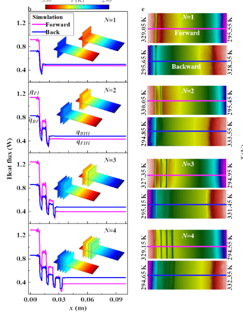
Figure 4: Theoretical, simulation and experimental results of non-reciprocal heat transport configurations with different numbers of vertical plates. (a) Shows the structural layout. (b) Depict simulation outcomes for configurations with 1, 2, 3, and 4 vertical plates, respectively. (c) and (d) Illustrate how heat flow values and the rectification ratio vary with different numbers $N$ of vertical plates. Simulated values are derived from Figure 4b. (e) Present the experimental temperature field distributions for each configuration with 1, 2, 3, and 4 different plates, respectively. (f) Offer a comparative analysis of the temperature distributions along the centerline of the base plate between the experimental data and simulation results. The parameters used in the simulation results are consistent with the experimental parameters.

The reconfigurable non-reciprocal heat transport can be achieved by placing different numbers of vertical plates on the base plate. Notably, the stainless steel sample with a thermal conductivity of $\kappa=16.3~{}\rm Wm^{-1}K^{-1}$ exhibits the highest rectification ratio and the most pronounced non-reciprocal effect in experiments. Thus, we use this material to investigate the impact of vertical plate number on rectification ratio. Figure 4a presents a schematic of stainless steel samples with varying numbers of vertical plates. Figure 4b display simulation results for different plate counts $N$, keeping other parameters consistent with Figure 3b. These results indicate that increasing the number of plates amplifies the difference in heat flow values. By comparing the forward and backward heat flow values with theoretical predictions and then calculating the rectification ratio (shown in Figures 4c-d), we find that both inflow and outflow rectification ratios are directly proportional to the number of plates. The rectification ratio changes significantly up to three plates but only slightly from three to four plates. This minor change is attributed to the fourth plate’s proximity to the center, where the difference in natural convection during forward and backward heat transport is minimal, thus contributing less to the rectification ratio. Figure 4e present experimental results under natural convection for the entire structure. A comparison between simulation and experimental temperature profiles along the centerline is shown in Figure 4f, using consistent parameters including a natural convection coefficient of $h=8~{}\rm Wm^{-2}K^{-1}$ and ambient temperature $T_{amb}=301.4$ K. The base plate’s surface temperature distribution and the centerline temperature profiles clearly demonstrate significant differences between forward and backward heat transport. As shown in Figure 4f, the disparity in temperature distribution grows with the number of plates, and the simulation and experimental results align closely. According to the simulation results, the inflow rectification ratio increases with the number of plates, while the outflow rectification ratio shows slight fluctuations. This is due to the lack of strict control over variables in the experiments, as the temperatures of the hot and cold sources are not entirely consistent in each trial. Under strict control of variables, the inflow and outflow rectification ratios of the stainless steel samples are directly proportional to the number of plates, as shown in Appendix I. Our study confirms that reconfigurable non-reciprocal heat transport is achievable by adjusting the thermal conductivity and number of vertical plates. This structure’s non-reciprocal heat transport can also be modulated by other factors, such as ambient temperature and the temperatures of the hot and cold sources. This structure allows for configurable non-reciprocal heat transport without altering its structure. It is evident that the non-reciprocal outcomes of this structure possess universality and robustness.

IV Conclusions

We successfully demonstrate the achievement of reconfigurable non-reciprocal heat transport using asymmetrical structure made of natural homogeneous materials, and leveraging natural convection. We have established a precise mathematical model that relates various parameters to the rectification ratio, revealing that optimal rectification can be attained through careful parameter adjustment. Specifically, we find that the rectification ratio is inversely proportional to the material’s thermal conductivity and directly proportional to the number of vertical plates used. The close correlation between our simulation results and experimental data robustly validates this relationship. By utilizing simple structural designs and natural convection processes, our research offers valuable insights for efficient thermal management and practical implementation in engineering designs.

V Methods

We employ Comsol Multiphysics software for our numerical simulations, using solid heat transport plates to model heat transport. Natural convection is simulated by applying convective heat flux to the surfaces of the structures. Specifically, in the designs illustrated in Figures 2b-i, 3b, and 4b, the surfaces at $x=0$ and $x=c$ are designated as cold and heat source surfaces, respectively. Convective heat flux is applied to all surfaces of the vertical plates, while other surfaces are set to thermal insulation. For the structures shown in Figures 3f and 4f, convective heat flux is applied to all surfaces except for those at $x=0$ and $x=c$.

The geometric parameters of the structure in Figure 3 and 4 are as follows: $c=0.1~{}\rm m$ and the structure’s width is 0.04 m. In the structure of Figure 3, the total length of the vertical plates is 0.042 m, symmetrically distributed on both sides of the base plate. The positions of the five vertical plates along the x-axis are 0.011 m, 0.018 m, 0.025 m, 0.032 m, and 0.039 m, each with a thickness of 0.002 m. The geometric parameters for the structure in Figure 4 are identical to those in Figure 3, with the only variation being the reduced number of vertical plates from the center position outwards.

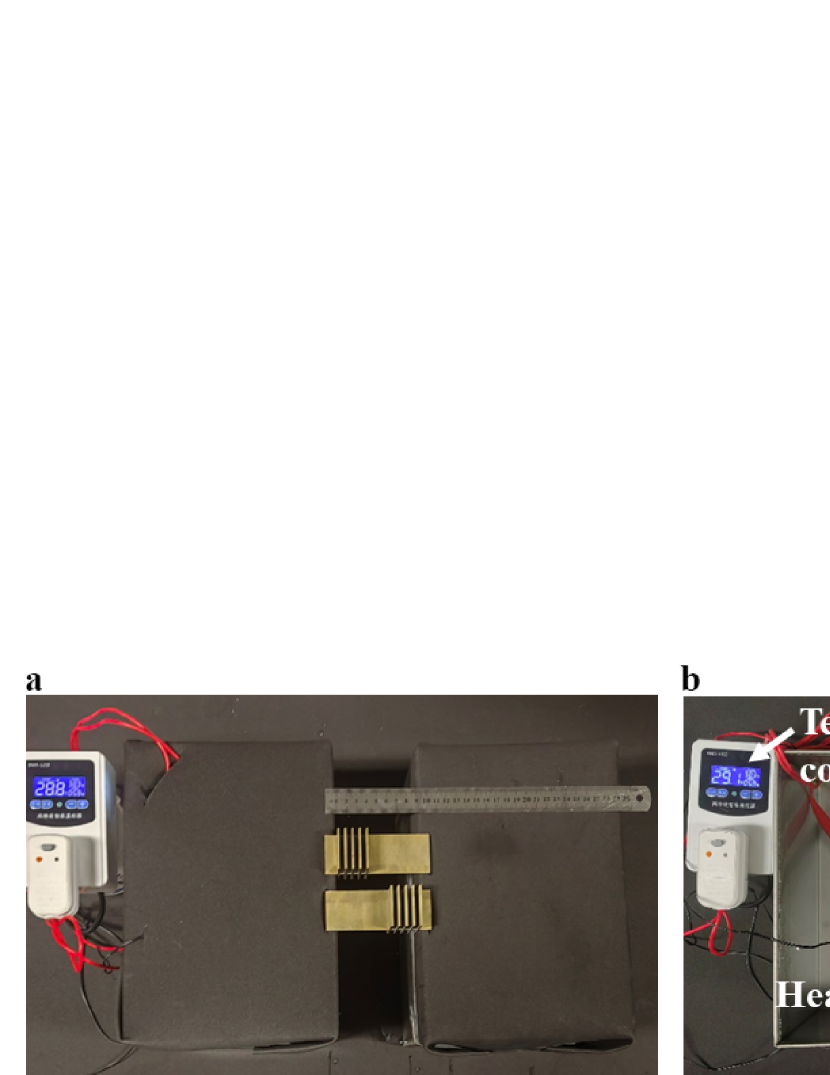
Figure A10: (a) Visual representation of the experimental device. (b) Shows the heat and cold source with the insulation film removed. (c) Schematic diagram of the experimental sample.

The experimental setup mirrors the shape and boundary conditions of the numerical simulations, as depicted in Figures 3a and 4a. The physical arrangement of the experiment is shown in Figure A10. In comparison to the simulated structure, both ends of the experimental structure are extended by 0.03 m and bent. These extensions are immersed in cold and hot water to replicate the temperatures of the cold and hot sources used in the simulations. A heating rod, regulated by a temperature controller, maintains the heat source at a constant temperature. The cold source is created using an ice-water mixture. For each experimental parameter, we use two identical samples, positioning the cold and heat sources in opposite directions to ensure consistent temperatures for both forward and backward heat transport. The experiments are conducted in an air-conditioned room to maintain a stable ambient temperature and minimize variations in the natural convection coefficient. By conducting experiments away from air outlets, we further ensure a consistent natural convection environment. To measure the natural convection coefficient, we heat a thin sheet of the same material in air and record its temperature profile. This data is then compared to a simulation set at the same temperature gradient. By adjusting the convection coefficient in the simulation until the experimental and simulated temperature profiles align, we are able to determine the accurate natural convection coefficient for our experimental conditions.

Appendix A. Theoretical calculation of the thermal field distribution of the non-reciprocal structure

The reconfigurable structure for non-reciprocal heat transport is depicted in Figure S1a, where a detailed view of the vertical plate is provided in Figure S1b. To determine the temperature distribution across the vertical plate, we apply the principles of energy conservation. Given the plate’s slender profile, temperature variations along the z-axis are significantly more pronounced than those along the x-axis, leading us to focus on one-dimensional heat transport in the z-direction. The structure, constructed from a homogeneous material, maintains a constant thermal conductivity ($\kappa$), and the heat convection coefficient ($h$) on its surface is uniformly distributed. We use a smooth metal substrate for the vertical plate, positioned in air. In this setup, the radiative heat transport is considerably less than the air’s convective heat transport. Consequently, our analysis primarily considers the heat conduction from the base plate to the vertical plate and the natural convection heat transport from the air to the plate.

Take a small element in the vertical plate with a length $dz$ in the z-axis. Due to Fourier’s law, the heat conduction rate at position $z$ can be written as

$$q_{z}=-\kappa A_{c}\frac{dT}{dz},$$ (A.1)

where $A_{c}$ is the cross-sectional area. The heat conduction rate at z+dz can be written as

$$q_{z+dz}=q_{z}+\frac{dq_{z}}{dz}dz.$$ (A.2)

The convective heat transport rate is given by

$$dq_{conv}=hdA_{s}(T-T_{amb}),$$ (A.3)

where $T_{amb}$ is ambient temperature, $A_{s}=Pdz$ is the surface area of the small element, and $P$ is the perimeter of the small element. Considering energy conservation in the small element, we have

$$q_{z}=q_{z+dz}+dq_{conv}.$$ (A.4)

Substituting Equations (A.1)-(A.3) into Equation (A.4), and $A_{c}$ is constant, we get

$$\frac{d^{2}T}{dz^{2}}-\frac{hP}{\kappa A_{c}}(T-T_{amb})=0.$$ (A.5)

Let $m^{2}=\frac{hP}{\kappa A_{c}}$ and $\theta(z)=T(z)-T_{amb}$, Equation (A.5) can be further simplified as

$$\begin{array}[]{c}\frac{d^{2}\theta}{dz^{2}}-m^{2}\theta=0.\end{array}$$ (A.6)

This is a linear, homogeneous, second-order differential equation with constant coefficients, and the general solution is

$$\theta(z)=d_{1}e^{mz}+d_{2}e^{-mz}.$$ (A.7)

Therefore, we can write the temperature distribution of the vertical plate as

$$T_{IV}(z)=T_{amb}+d_{1}e^{mz}+d_{2}e^{-mz},$$ (A.8)

where $d_{1}$ and $d_{2}$ are constants.

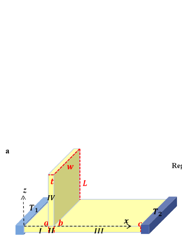
Figure A1: (a) Structural diagram of reconfigurable nonreciprocal heat transport. (b) Magnified view of Area IV.

We provide a general solution for the thermal field distribution across all four regions.

$$\begin{array}[]{c}T_{I}(x)=c_{1}x+c_{2},\\ T_{II}(x)=c_{3}x+c_{4},\\ T_{III}(x)=c_{5}x+c_{6},\\ T_{IV}(z)-T_{amb}=d_{1}e^{mz}+d_{2}e^{-mz},\end{array}$$ (A.9)

where $c_{1},c_{2},c_{3},c_{4},c_{5},c_{6},d_{1},d_{2}$ are unknown constants, which can be found through the continuity of temperature and heat flow at the boundary. The boundary conditions on the contact surface of the four regions can be written as

$$\begin{array}[]{c}c_{2}=T_{1},\\ c_{1}a+c_{2}=c_{3}a+c_{4},\\ c_{3}b+c_{4}=c_{5}b+c_{6},\\ c_{5}c+c_{6}=T_{2},\\ c_{1}a+c_{2}-T_{amb}=d_{1}+d_{2},\\ -\kappa Ac_{1}=-\kappa Ac_{3}-\kappa A_{c}m(d_{1}-d_{2}),\\ -\kappa Ac_{3}=-\kappa Ac_{5},\\ hA_{c}(d_{1}e^{mL}+d_{2}e^{-mL})=-\kappa A_{c}m(d_{1}e^{mL}-d_{2}e^{-mL}).\end{array}$$ (A.10)

Here the positions of the contact surfaces between Area I and II, and Area II and III are denoted as $a$ and $b$, respectively. The base plate’s length is $c$, with a cross-sectional area $A$. The vertical plate has a cross-sectional area $A_{c}$ and a height $L$, as illustrated in Figure S1. The parameter, $m=\sqrt{hP/(\kappa A_{c})}$, involves the natural convection coefficient $h$, the thermal conductivity $\kappa$, and the perimeter $P$ of the vertical plate’s top edge. Equation (A.10) details the temperature relationships at various contact surfaces, indicating different heat flow paths in the structure. Specifically, the fifth equation asserts that the temperature at the contact surface between Region II and IV ($z=0$) equals that between Region I and II ($x=a$). The sixth equation describes the division of heat flow from Area I into Areas II and IV, while the eighth equation presents the boundary condition at the contact surface between Area IV’s top edge ($z=L$) and the air. Solving these eight boundary conditions can yield the temperature distribution of the entire structure.

By solving Equation (A.10), we can obtain the temperature field and heat flow distribution of the entire structure, the results of which are shown in Figures 2b-c of the main text. Both the theoretical and simulation studies use the same parameters, namely $\kappa=16.3~{}\rm Wm^{-1}K^{-1}$, $h=20~{}\rm Wm^{-2}K^{-1}$, $T_{1}=373~{}\rm K$ and $T_{2}=273~{}\rm K$, $T_{amb}=298~{}\rm K$, $L=0.04~{}\rm m$, $a=0.01~{}\rm m$, $b=0.012~{}\rm m$, $c=0.1~{}\rm m$, and the structure’s width is 0.04 m.

Appendix B. Simulation results: Non-reciprocal structures with varied thermal conductivities

This section presents the simulation outcomes of the non-reciprocal effect, emphasizing its dependence on varying thermal conductivity ratios, as illustrated in Figure S2. We conduct simulations using five different materials, each with distinct thermal conductivities. The results of these simulations are displayed in Figures S2b-f. The simulations are standardized with the following parameters: heat convection coefficient $h=20~{}\rm Wm^{-2}K^{-1}$, temperatures $T_{1}=373~{}\rm K$ and $T_{2}=273~{}\rm K$, ambient temperature $T_{amb}=298~{}\rm K$, and dimensions $L=0.04~{}\rm m$, $a=0.01~{}\rm m$, $b=0.012~{}\rm m$, and $c=0.1~{}\rm m$. The temperature distribution diagrams clearly demonstrate the non-reciprocal effects. Notably, as thermal conductivity escalates, the vertical plate’s temperature increasingly aligns with the base plate’s median temperature in both forward and backward scenarios. Consequently, the disparity in natural convection, both forward and backward, diminishes with higher thermal conductivity. This trend is also evident in the heat flow diagrams, where the differences in forward and backward heat flows decrease with increasing thermal conductivity, suggesting a reduction in the vertical plate’s natural convection. These observations culminate in an inverse relationship between the rectification ratio and thermal conductivity. The heat flow values extracted from Figures S2b-f are further consolidated and presented in Figure S2a.

Appendix C. Theoretical analysis and simulation outcomes for non-reciprocal structures with varied numbers of vertical plates

By adjusting the number of vertical plates, we can tailor the rectification ratio to our needs. Figure S3 presents both structural schematics and simulation results for configurations with different numbers of vertical plates. The structure in Figure S3a aligns with that of Figure 2a from the main text. We introduce a revised region nomenclature, replacing regions I-IV with A-D. The theoretical analysis for Figure S3a is detailed in the Section 1, while the analysis for Figure S3b follows a similar methodology, the key difference being the addition of three more areas. The thermal field distribution in 7 regions can be written as

$$\begin{array}[]{c}T_{A}(x)=c_{1}x+c_{2},T_{B}(x)=c_{3}x+c_{4},\\ T_{C}(x)=c_{5}x+c_{6},T_{D}(x)=c_{7}x+c_{8},\\ T_{E}(x)=c_{9}x+c_{10},T_{F}(z)-T_{amb}=d_{1}e^{mz}+d_{2}e^{-mz},\\ T_{G}(z)-T_{amb}=d_{3}e^{mz}+d_{4}e^{-mz},\end{array}$$ (A.11)

where $c_{1}-c_{10},d_{1}-d_{4}$ are unknown constants. The boundary conditions on the contact surface can be written as

$$\begin{array}[]{c}c_{2}=T_{1},c_{9}c+c_{10}=T_{2},\\ c_{1}a_{1}+c_{2}=c_{3}a_{1}+c_{4},c_{3}b_{1}+c_{4}=c_{5}b_{1}+c_{6},\\ c_{5}a_{2}+c_{6}=c_{7}a_{2}+c_{8},c_{7}b_{2}+c_{8}=c_{9}b_{2}+c_{10},\\ c_{1}a_{1}+c_{2}-T_{amb}=d_{1}+d_{2},c_{5}a_{2}+c_{6}-T_{amb}=d_{3}+d_{4},\\ -\kappa Ac_{1}=-\kappa Ac_{3}-\kappa A_{c}m(d_{1}-d_{2}),-\kappa Ac_{5}=-\kappa Ac_{7}-\kappa A_{c}m(d_{3}-d_{4}),\\ -\kappa Ac_{3}=-\kappa Ac_{5},-\kappa Ac_{7}=-\kappa Ac_{9},\\ hA_{c}(d_{1}e^{mL}+d_{2}e^{-mL})=-\kappa A_{c}m(d_{1}e^{mL}-d_{2}e^{-mL}),\\ hA_{c}(d_{3}e^{mL}+d_{4}e^{-mL})=-\kappa A_{c}m(d_{3}e^{mL}-d_{4}e^{-mL}),\end{array}$$ (A.12)

where $a_{1}$ and $b_{1}$ are the starting and ending positions of the first vertical board, and $a_{2}$ and $b_{2}$ are the second vertical board. There are 14 unknowns and 14 boundary conditions. These simultaneous boundary conditions are essential for determining the thermal field distribution across the entire structure. For calculating the rectification ratio, we focus on the heat flow values in areas A and E. Notably, the addition of each vertical plate introduces 3 new areas, 6 additional unknowns, and necessitates 6 more boundary conditions. This pattern is consistently applied to each vertical plate in the structure. At the point where $z=0$, the temperature equals that of the contact surface between the base and the vertical plate, allowing a portion of the heat flow from the base plate to transport into the vertical plate.

The non-reciprocal structure of three vertical plates can be divided into 10 areas, and the thermal field distribution is written as

$$\begin{array}[]{c}T_{A}(x)=c_{1}x+c_{2},T_{B}(x)=c_{3}x+c_{4},\\ T_{C}(x)=c_{5}x+c_{6},T_{D}(x)=c_{7}x+c_{8},\\ T_{E}(x)=c_{9}x+c_{10},T_{F}(x)=c_{11}x+c_{12},\\ T_{G}(x)=c_{13}x+c_{14},T_{H}(z)-T_{amb}=d_{1}e^{mz}+d_{2}e^{-mz},\\ T_{I}(z)-T_{amb}=d_{3}e^{mz}+d_{4}e^{-mz},T_{J}(z)-T_{amb}=d_{5}e^{mz}+d_{6}e^{-mz}.\end{array}$$ (A.13)

The 20 boundary conditions are written as

$$\begin{array}[]{c}c_{2}=T_{1},c_{13}c+c_{14}=T_{2},\\ c_{1}a_{1}+c_{2}=c_{3}a_{1}+c_{4},c_{3}b_{1}+c_{4}=c_{5}b_{1}+c_{6},\\ c_{5}a_{2}+c_{6}=c_{7}a_{2}+c_{8},c_{7}b_{2}+c_{8}=c_{9}b_{2}+c_{10},\\ c_{9}a_{3}+c_{10}=c_{11}a_{3}+c_{12},c_{11}b_{3}+c_{12}=c_{13}b_{3}+c_{14},\\ c_{1}a_{1}+c_{2}-T_{amb}=d_{1}+d_{2},c_{5}a_{2}+c_{6}-T_{amb}=d_{3}+d_{4},\\ c_{9}a_{3}+c_{10}-T_{amb}=d_{5}+d_{6},-\kappa Ac_{1}=-\kappa Ac_{3}-\kappa A_{c}m(d_{1}-d_{2}),\\ -\kappa Ac_{5}=-\kappa Ac_{7}-\kappa A_{c}m(d_{3}-d_{4}),-\kappa Ac_{9}=-\kappa Ac_{11}-\kappa A_{c}m(d_{5}-d_{6}),\\ -\kappa Ac_{3}=-\kappa Ac_{5},-\kappa Ac_{7}=-\kappa Ac_{9},-\kappa Ac_{11}=-\kappa Ac_{13},\\ hA_{c}(d_{1}e^{mL}+d_{2}e^{-mL})=-\kappa A_{c}m(d_{1}e^{mL}-d_{2}e^{-mL}),\\ hA_{c}(d_{3}e^{mL}+d_{4}e^{-mL})=-\kappa A_{c}m(d_{3}e^{mL}-d_{4}e^{-mL}),\\ hA_{c}(d_{5}e^{mL}+d_{6}e^{-mL})=-\kappa A_{c}m(d_{5}e^{mL}-d_{6}e^{-mL}).\end{array}$$ (A.14)

The thermal field distribution and boundary conditions of the non-reciprocal structure of four vertical plates can be written as Equations (A.15) and(A.16),

$$\begin{array}[]{c}T_{A}(x)=c_{1}x+c_{2},T_{B}(x)=c_{3}x+c_{4},\\ T_{C}(x)=c_{5}x+c_{6},T_{D}(x)=c_{7}x+c_{8},\\ T_{E}(x)=c_{9}x+c_{10},T_{F}(x)=c_{11}x+c_{12},\\ T_{G}(x)=c_{13}x+c_{14},T_{H}(x)=c_{15}x+c_{16},\\ T_{I}(x)=c_{17}x+c_{18},T_{J}(z)-T_{amb}=d_{1}e^{mz}+d_{2}e^{-mz},\\ T_{K}(z)-T_{amb}=d_{3}e^{mz}+d_{4}e^{-mz},T_{L}(z)-T_{amb}=d_{5}e^{mz}+d_{6}e^{-mz},\\ T_{M}(z)-T_{amb}=d_{7}e^{mz}+d_{8}e^{-mz},\end{array}$$ (A.15)

and

$$\begin{array}[]{c}c_{2}=T_{1},c_{17}c+c_{18}=T_{2},\\ c_{1}a_{1}+c_{2}=c_{3}a_{1}+c_{4},c_{3}b_{1}+c_{4}=c_{5}b_{1}+c_{6},\\ c_{5}a_{2}+c_{6}=c_{7}a_{2}+c_{8},c_{7}b_{2}+c_{8}=c_{9}b_{2}+c_{10},\\ c_{9}a_{3}+c_{10}=c_{11}a_{3}+c_{12},c_{11}b_{3}+c_{12}=c_{13}b_{3}+c_{14},\\ c_{13}a_{4}+c_{14}=c_{15}a_{4}+c_{16},c_{15}b_{4}+c_{16}=c_{17}b_{4}+c_{18},\\ c_{1}a_{1}+c_{2}-T_{amb}=d_{1}+d_{2},c_{5}a_{2}+c_{6}-T_{amb}=d_{3}+d_{4},\\ c_{9}a_{3}+c_{10}-T_{amb}=d_{5}+d_{6},c_{13}a_{4}+c_{14}-T_{amb}=d_{7}+d_{8},\\ -\kappa Ac_{1}=-\kappa Ac_{3}-\kappa A_{c}m(d_{1}-d_{2}),-\kappa Ac_{5}=-\kappa Ac_{7}-\kappa A_{c}m(d_{3}-d_{4}),\\ -\kappa Ac_{9}=-\kappa Ac_{11}-\kappa A_{c}m(d_{5}-d_{6}),-\kappa Ac_{13}=-\kappa Ac_{15}-\kappa A_{c}m(d_{7}-d_{8}),\\ -\kappa Ac_{3}=-\kappa Ac_{5},-\kappa Ac_{7}=-\kappa Ac_{9},-\kappa Ac_{11}=-\kappa Ac_{13},-\kappa Ac_{15}=-\kappa Ac_{17},\\ hA_{c}(d_{1}e^{mL}+d_{2}e^{-mL})=-\kappa A_{c}m(d_{1}e^{mL}-d_{2}e^{-mL}),\\ hA_{c}(d_{3}e^{mL}+d_{4}e^{-mL})=-\kappa A_{c}m(d_{3}e^{mL}-d_{4}e^{-mL}),\\ hA_{c}(d_{5}e^{mL}+d_{6}e^{-mL})=-\kappa A_{c}m(d_{5}e^{mL}-d_{6}e^{-mL}),\\ hA_{c}(d_{7}e^{mL}+d_{8}e^{-mL})=-\kappa A_{c}m(d_{7}e^{mL}-d_{8}e^{-mL}).\end{array}$$ (A.16)

The thermal field distribution and boundary conditions of the non-reciprocal structure of five vertical plates can be written as Equations (A.17) and(A.18),

$$\begin{array}[]{c}T_{A}(x)=c_{1}x+c_{2},T_{B}(x)=c_{3}x+c_{4},\\ T_{C}(x)=c_{5}x+c_{6},T_{D}(x)=c_{7}x+c_{8},\\ T_{E}(x)=c_{9}x+c_{10},T_{F}(x)=c_{11}x+c_{12},\\ T_{G}(x)=c_{13}x+c_{14},T_{H}(x)=c_{15}x+c_{16},\\ T_{I}(x)=c_{17}x+c_{18},T_{J}(x)=c_{19}x+c_{20},\\ T_{K}(x)=c_{21}x+c_{22},T_{L}(z)-T_{amb}=d_{1}e^{mz}+d_{2}e^{-mz},\\ T_{M}(z)-T_{amb}=d_{3}e^{mz}+d_{4}e^{-mz},T_{N}(z)-T_{amb}=d_{5}e^{mz}+d_{6}e^{-mz},\\ T_{O}(z)-T_{amb}=d_{7}e^{mz}+d_{8}e^{-mz},T_{P}(z)-T_{amb}=d_{9}e^{mz}+d_{10}e^{-mz},\end{array}$$ (A.17)

and

$$\begin{array}[]{c}c_{2}=T_{1},c_{21}c+c_{22}=T_{2},\\ c_{1}a_{1}+c_{2}=c_{3}a_{1}+c_{4},c_{3}b_{1}+c_{4}=c_{5}b_{1}+c_{6},\\ c_{5}a_{2}+c_{6}=c_{7}a_{2}+c_{8},c_{7}b_{2}+c_{8}=c_{9}b_{2}+c_{10},\\ c_{9}a_{3}+c_{10}=c_{11}a_{3}+c_{12},c_{11}b_{3}+c_{12}=c_{13}b_{3}+c_{14},\\ c_{13}a_{4}+c_{14}=c_{15}a_{4}+c_{16},c_{15}b_{4}+c_{16}=c_{17}b_{4}+c_{18},\\ c_{17}a_{5}+c_{18}=c_{19}a_{5}+c_{20},c_{19}b_{5}+c_{20}=c_{21}b_{4}+c_{22},\\ c_{1}a_{1}+c_{2}-T_{amb}=d_{1}+d_{2},c_{5}a_{2}+c_{6}-T_{amb}=d_{3}+d_{4},\\ c_{9}a_{3}+c_{10}-T_{amb}=d_{5}+d_{6},c_{13}a_{4}+c_{14}-T_{amb}=d_{7}+d_{8},\\ c_{17}a_{5}+c_{18}-T_{amb}=d_{9}+d_{10},-\kappa Ac_{1}=-\kappa Ac_{3}-\kappa A_{c}m(d_{1}-d_{2}),\\ -\kappa Ac_{5}=-\kappa Ac_{7}-\kappa A_{c}m(d_{3}-d_{4}),-\kappa Ac_{9}=-\kappa Ac_{11}-\kappa A_{c}m(d_{5}-d_{6}),\\ -\kappa Ac_{13}=-\kappa Ac_{15}-\kappa A_{c}m(d_{7}-d_{8}),-\kappa Ac_{17}=-\kappa Ac_{19}-A_{c}\kappa m(d_{9}-d_{10}),\\ -\kappa Ac_{3}=-\kappa Ac_{5},-\kappa Ac_{7}=-\kappa Ac_{9},-\kappa Ac_{11}=-\kappa Ac_{13},-\kappa Ac_{15}=-\kappa Ac_{17},-\kappa Ac_{19}=-\kappa Ac_{21},\\ hA_{c}(d_{1}e^{mL}+d_{2}e^{-mL})=-\kappa A_{c}m(d_{1}e^{mL}-d_{2}e^{-mL}),\\ hA_{c}(d_{3}e^{mL}+d_{4}e^{-mL})=-\kappa A_{c}m(d_{3}e^{mL}-d_{4}e^{-mL}),\\ hA_{c}(d_{5}e^{mL}+d_{6}e^{-mL})=-\kappa A_{c}m(d_{5}e^{mL}-d_{6}e^{-mL}),\\ hA_{c}(d_{7}e^{mL}+d_{8}e^{-mL})=-\kappa A_{c}m(d_{7}e^{mL}-d_{8}e^{-mL}),\\ hA_{c}(d_{9}e^{mL}+d_{10}e^{-mL})=-\kappa A_{c}m(d_{9}e^{mL}-d_{10}e^{-mL}).\end{array}$$ (A.18)

The simulation results corresponding to five plate numbers are shown in Figures S3f-j. The simulation parameters and theoretical parameters are both set to $\kappa=200~{}\rm Wm^{-1}K^{-1}$, $h=20~{}\rm Wm^{-2}K^{-1}$, $T_{1}=373~{}\rm K$, $T_{2}=273~{}\rm K$, $T_{amb}=298~{}\rm K$, $L=0.04~{}\rm m$, $a_{1}=0.01~{}\rm m$, $a_{2}=0.017~{}\rm m$, $a_{3}=0.024~{}\rm m$, $a_{4}=0.031~{}\rm m$, $a_{5}=0.038~{}\rm m$, $b_{1}=0.012~{}\rm m$, $b_{2}=0.019~{}\rm m$, $b_{3}=0.026~{}\rm m$, $b_{4}=0.033~{}\rm m$, $b_{5}=0.04~{}\rm m$ and $c=0.1~{}\rm m$. Theoretical and simulated inflow and outflow heat flow values are shown in Figure S3k. In this case, the rectification ratio is proportional to the number of vertical plates.

Appendix D. Interplay of thermal conductivity and number of vertical plates in determining the rectification ratio

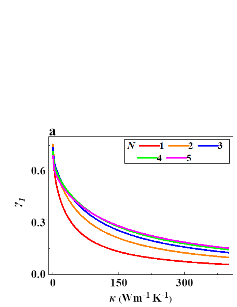
Figure A4: (a) and (b) Show how the inflow and outflow rectification ratios vary with both thermal conductivity $\kappa$ and the number $N$ of vertical plates. (c) Depicts the variation of the rectification ratio with plate numbers under different thermal conductivities.

The correlation between the rectification ratio and the number of vertical plates is intricately tied to the material’s thermal conductivity. Figures S4a and b illustrate the theoretical variation of the rectification ratio with thermal conductivity across different numbers of vertical plates. All parameters, except for thermal conductivity, remain consistent with those in Figure S3. It’s observed that the trends of decreasing inflow and outflow rectification ratios with increasing thermal conductivity remain constant, irrespective of the number of plates. However, the specific relationship between the rectification ratio and the number of plates varies with different thermal conductivities. Analyzing five sets of thermal conductivity values, ranging from low to high, Figure S4c demonstrates the fluctuating rectification ratio in response to the number of plates. At a thermal conductivity of $\kappa=0.1~{}\rm Wm^{-1}K^{-1}$, the rectification ratio peaks when there’s only one vertical plate, showcasing the most pronounced non-reciprocal effect. As thermal conductivity increases, the number of plates yielding the maximum rectification ratio shifts progressively from the second to the fifth plate. In backward heat transport, the vertical plate’s temperature is usually lower than the ambient, low thermal conductivity results in a high inward natural convection. Conversely, in the forward direction with low thermal conductivity, the temperature near the base plate’s center can drop below ambient, reducing overall external natural convection. Hence, the relationship between the rectification ratio and the number of plates is not uniformly monotonic but varies depending on the thermal conductivity.

Appendix E. Variation of rectification ratio with vertical plate height

Figure S5 presents both theoretical and simulation results demonstrating the influence of vertical plate height on the rectification ratio. The parameters for these analyses are set as follows: thermal conductivity $\kappa=16.3~{}\rm Wm^{-1}K^{-1}$, heat convection coefficient $h=20~{}\rm Wm^{-2}K^{-1}$, temperatures $T_{1}=373~{}\rm K$ and $T_{2}=273~{}\rm K$, ambient temperature $T_{amb}=298~{}\rm K$, and dimensions $a=0.01~{}\rm m$, $b=0.012~{}\rm m$, and $c=0.1~{}\rm m$. Analysis of Figure S5a reveals that the heat flow in Area I, both forward and backward, intensifies with an increase in vertical plate height, eventually stabilizing at a constant value, while heat flow in Area III diminishes. Consequently, the rectification ratios for both inflow and outflow rise in correlation with the height of the vertical plate. The close alignment of the simulation data points with the theoretical solid line corroborates the accuracy of the theoretical framework.

As depicted in Figures S5g-i, the integration of the vertical plate through the base plate not only enhances structural stability but also amplifies the rectification ratio. With the vertical plates symmetrically positioned relative to the base plate, their temperature distributions on either side of the base are consistent. In theoretical modeling, this only requires modifying the sixth equation of Equation (A.10) to $-\kappa Ac_{1}=-\kappa Ac_{3}-2\kappa A_{c}m(d_{1}-d_{2})$ for calculating both inflow and outflow heat flows. Figure S5g indicates that for equal total lengths of vertical plates, the penetration approach increases forward inflow (FI) and reverse outflow (BI) heat flow values while decreasing reverse inflow (BIII) and forward outflow (FIII) values. Consequently, as shown in Figure S5i, the penetration method effectively enhances both the inflow and outflow rectification ratios.

Appendix F. Impact of vertical plate position on rectification ratio

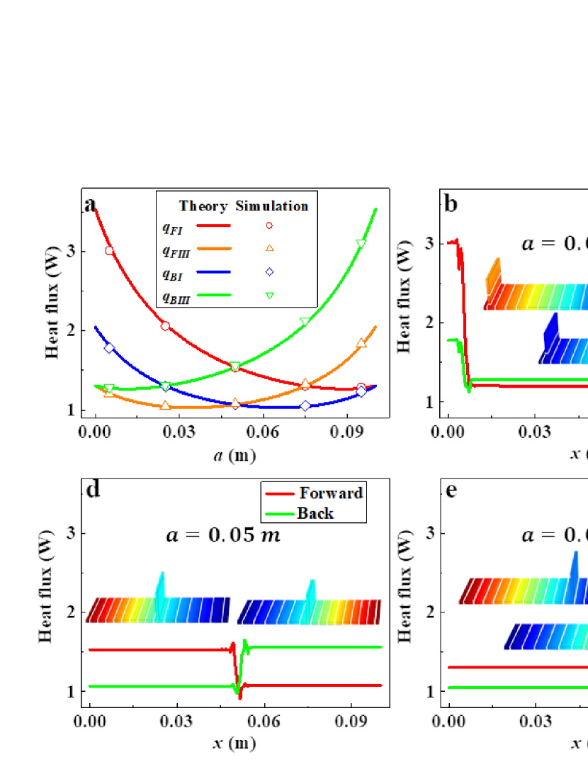
Figure A6: (a) Show how heat flow values vary with changes in the vertical plate’s position $a$. (b) to (f) Present simulated temperature profiles and heat flow diagrams corresponding to the data points in panel (a), with vertical plate positions at $a=$ 0.005 m, 0.025 m, 0.05 m, 0.075 m, and 0.095 m.

Figure S6 illustrates both theoretical and simulation analyses of how the rectification ratio varies with the position of the vertical plate. In these studies, the vertical plate’s height is fixed at 0.02 m, with all other parameters aligned with those in Figure S5a. The theoretical and simulation outcomes show remarkable consistency. The rectification ratio increases as the vertical plate’s position moves further from the center. Notably, when the vertical plate is centered on the base plate, the rectification ratio is zero, signifying reciprocal heat transport at this position. This finding underscores that asymmetric structure and natural convection are crucial elements for achieving non-reciprocal heat transport.

Appendix G. Variation of rectification ratio with ambient temperature

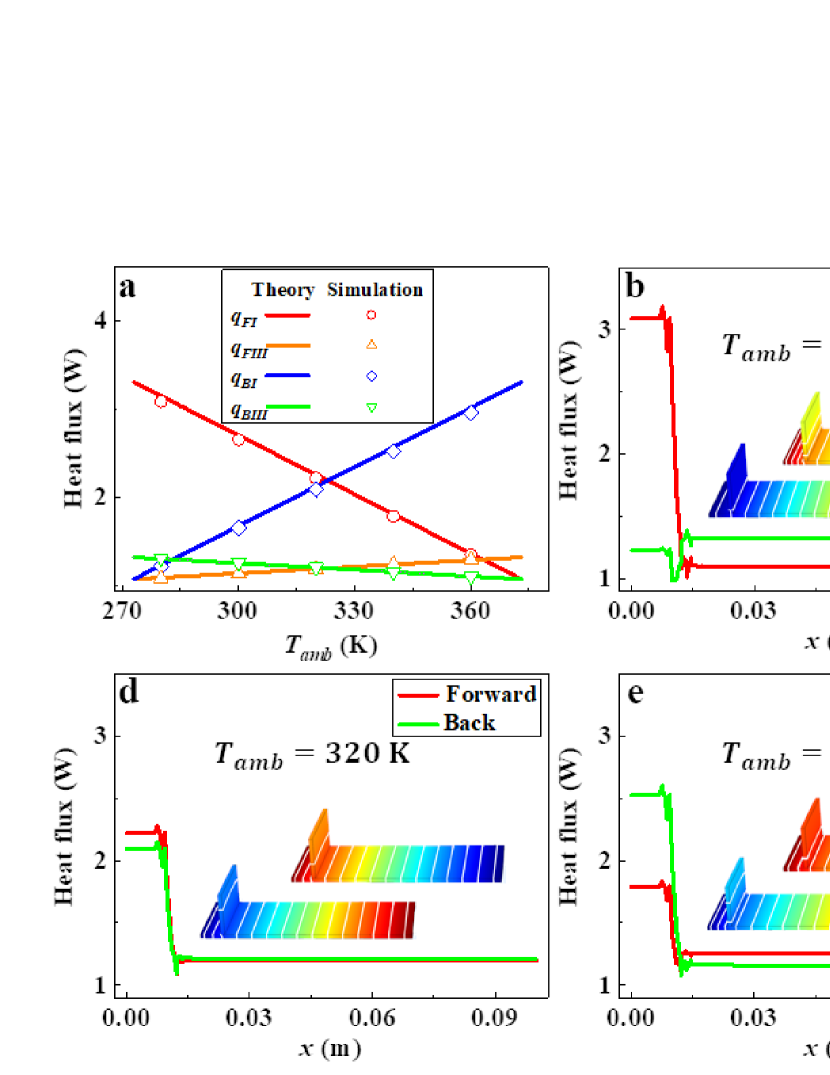
Figure A7: (a) Illustrate how both heat flow values vary with changes in ambient temperature $T_{amb}$. (b) to (f) Feature simulated temperature profiles and heat flow diagrams for ambient temperatures at 280 K, 300 K, 320 K, 340 K, and 360 K.

Figure S7 demonstrates that, within a constant non-reciprocal structure, the rectification ratio can be modulated by adjusting the ambient temperature. Maintaining the same parameters as in Figure S6, except for the ambient temperature, we observe that the inflow and outflow heat flow values exhibit a linear relationship with the ambient temperature. An increase in ambient temperature diminishes the natural convection heat transport from the vertical plate to the air in the forward direction, while it enhances it in the reverse direction. Consequently, with rising ambient temperatures, the inflow rectification ratio decreases, and the outflow rectification ratio increases.

Appendix H. Influence of temperature difference between hot and cold sources on rectification ratio

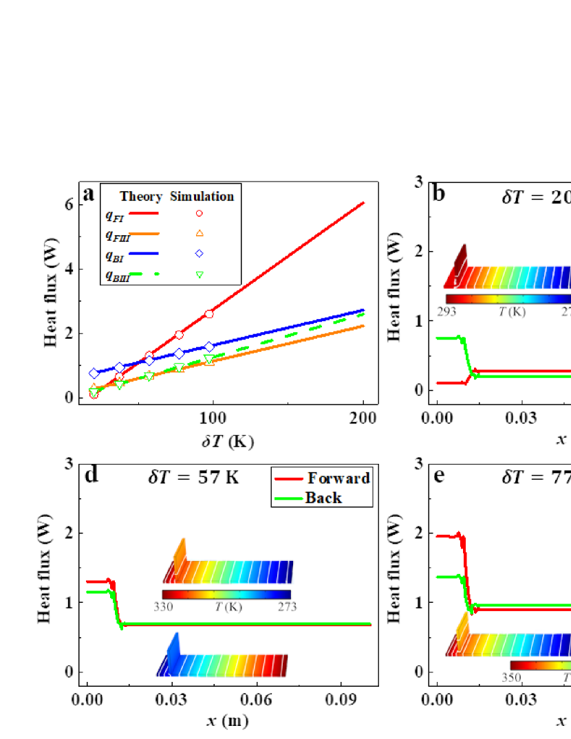
Figure A8: (a) Showcase the variation in heat flow values with $\delta T=|T_{1}-T_{2}|$. (b) to (f) Display simulated temperature profiles and heat flow diagrams for temperature differences of 20 K, 37 K, 57 K, 77 K, and 97 K.

The rectification ratio is notably influenced by the temperature differential between the hot and cold sources, as illustrated in Figure S8. With the ambient temperature held at 298 K and a constant $T_{1}$ of 273 K, altering $T_{2}$ varies the temperature difference $\delta T$. As $\delta T$ increases, the outflow rectification ratio first decreases then stabilizes. Conversely, the inflow rectification ratio initially drops from a high value before increasing. This pattern is attributed to changes in the forward heat flow distribution with varying $\delta T$. When the non-reciprocal structure’s overall temperature is below ambient, air warms the vertical plate, reducing heat flow in area I compared to area III in the forward direction, as depicted in Figure S8b. However, as $\delta T$ rises, air’s impact on the vertical plate lessens in the forward direction, causing a decrease in the inflow rectification ratio. In cases where the vertical plate’s temperature exceeds ambient, air cools the vertical plate, resulting in higher heat flow in area I than in area III, as seen in Figures S8c-f. Here, increasing $\delta T$ intensifies natural convection between the air and the vertical plate, leading to a rise in the inflow rectification ratio.

Appendix I. Effect of air’s natural convection on the base plate in non-reciprocal heat transport

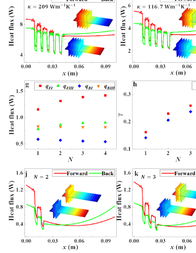
Figure A9: (a) and (b) The heat flow value and rectification ratio change with the thermal conductivity when the entire structure has natural convection. (c)-(f) Simulated thermal field and heat flow distributions for four different materials: copper (c), aluminum alloy (d), brass (e), and stainless steel (f). (g) and (h) The heat flow value and rectification ratio change with the number of vertical plates when the entire structure has natural convection. (i)-(l) Simulated thermal field and heat flow distributions for structures with different numbers of vertical plates ($N$=1, 2, 3, and 4).

Simulation results incorporating natural convection on the base plate are presented in Figure S9. These simulations use the structure from Figure 3b and 4b in the main text, with identical parameters. The key difference here is the inclusion of natural convection with air across the entire structure. The trends in heat flow value and rectification ratio as a function of thermal conductivity are consistent with those observed in Figure 3c-d. Figures S9c-f highlights the prominent non-reciprocal heat transport effects. It’s evident that the presence of natural convection on the base plate does not alter the fundamental non-reciprocal heat transport behavior but rather affects its magnitude. While the rectification ratio is higher without natural convection on the base plate when examining inflow and outflow heat flow values alone, the non-reciprocal effect is more pronounced when considering the overall heat flow distribution on the base plate with natural convection. Figures S9g-h are the results of heat flow values and rectification ratios under different numbers of vertical plates. The changing trends are consistent with Figures 4c-d of the main text.

Appendix J. Physical picture of the experimental setup

In our experimental setup, we cover the cold and heat sources with thermal insulation films to mitigate the influence of water vapor on the surrounding air, as illustrated in Figure S10. For clarity, we provide a diagram of the experimental device with the insulation film removed, detailing the specific arrangement.