Generalized Symmetries in 2D from String Theory: SymTFTs, Intrinsic Relativeness, and Anomalies of Non-invertible Symmetries

Abstract

Generalized global symmetries, in particular non-invertible and categorical symmetries, have become a focal point in the recent study of quantum field theory (QFT). In this paper, we investigate aspects of symmetry topological field theories (SymTFTs) and anomalies of non-invertible symmetries for 2D QFTs from a string theory perspective. Our primary focus is on an infinite class of 2D QFTs engineered on D1-branes probing toric Calabi-Yau 4-fold singularities. We derive 3D SymTFTs from the topological sector of IIB supergravity and discuss the resulting 2D QFTs, which can be intrinsically relative or absolute. For intrinsically relative QFTs, we propose a sufficient condition for them to exist. For absolute QFTs, we show that they exhibit non-invertible symmetries with an elegant brane origin. Furthermore, we find that these non-invertible symmetries can suffer from anomalies, which we discuss from a top-down perspective. Explicit examples are provided, including theories for $Y^{(p,k)}(\mathbb{P}^{2})$, $Y^{(2,0)}(\mathbb{P}^{1}\times\mathbb{P}^{1})$, and ${\mathbb{C}}^{4}/{\mathbb{Z}}_{4}$ geometries.

1 Introduction

The study of generalized global symmetries [1] has been instrumental in advancing our understanding of quantum field theory (QFT) and string theory. Notably, generalized global symmetries, including non-invertible symmetries, are ubiquitous in 2D QFTs, garnering significant attention over the past several years (see, for instance, [2, 3, 4, 5, 6, 7, 8, 9]). Non-invertible symmetries are described by the mathematical notion of (higher) fusion categories (see, e.g., [10]), thus they are sometimes also referred to as categorical symmetries.

A useful approach for investigating categorical symmetries is to extend the 2D spacetime manifold into a 3D bulk, where a topological field theory (TFT) lives. This methods works due to the topological nature of generalized global symmetries, which are symmetries captured by topological operators in QFTs [1]. Such topological information is encoded in the 3D TFT with two boundaries. One of the boundaries is physical, containing all local information of the 2D theory one is interested in, whereas the other boundary is topological and determines boundary conditions. This construction allows the decoupling of the global structure of a 2D QFT from its complicated local information, providing a clean approach to generalized global symmetries. The 3D bulk TFT is now commonly referred to as a symmetry TFT (SymTFT) (see, e.g., [11, 12, 13, 14, 3, 15, 16, 17, 18, 19]).

In many cases, the 3D bulk is auxiliary. This is because it is possible to move the topological boundary, merge it with the physical boundary, and thereby achieve a genuine 2D system. However, there are cases where the 3D TFT does not admit any topological boundary condition, so it is not possible to collapse the 3D bulk into a 2D system. The 3D TFT is now intrinsic, instead of auxiliary, and the corresponding 2D theory living on the physical boundary is known as a relative QFT [19]. In many works in literature, the term “relative QFT” is frequently also employed to indicate the physical boundary theory of the SymTFT with a topological boundary. To avoid ambiguity, in this paper we introduce the notion of intrinsically relative QFT to denote a theory whose bulk TFT does not admit any topological boundary condition. In other words, the bulk TFT is intrinsic instead of auxiliary.

When the SymTFT bulk admits a topological boundary, the 2D system obtained via shrinking the bulk is called an absolute QFT. If a SymTFT admits multiple boundary conditions, it will have multiple absolute QFT descendants, which are connected via topological manipulations, e.g., finite gauging and stacking local counterterms/SPT phases. This leads to a powerful aspect of the SymTFT, namely it can capture the anomalies for non-invertible symmetries. Consider an absolute QFT associated with a certain topological boundary condition for the SymTFT with a non-invertible symmetry. An attempt to gauge this symmetry would amount to changing the topological boundary condition. If the new boundary condition is not allowed by the SymTFT, then we end up with an obstruction to gauging, which corresponds to a ’t Hooft anomaly for the non-invertible symmetry (see, e.g., [36, 37, 38, 39]).

A powerful perspective for studying QFTs and their symmetries involves embedding them into string theory. Several works have been devoted to building generalized global symmetries from a top-down perspective in QFTs that admit a string theory realization via geometry engineering or brane probes. There are two primary questions in this approach: how to build topological symmetry operators and how to derive the SymTFTs. For a QFT engineered at a conical singularity $Y$, topological symmetry operators originate from either branes wrapping cycles “at infinity” along $\partial Y$ [40, 41, 42] (see also [43, 44, 45, 46, 47, 48]), or geometric fibers degenerated “at infinity” [49]. The non-topological dynamics of these asymptotic boundary objects (branes or fibers) is decoupled from the QFT localized at the conical singularity, but its topological effects remain. The SymTFT for the QFT, on the other hand, is obtained from the dimensional reduction of the topological sector of 10D/11D supergravity actions along the asymptotic boundary $\partial Y$ [50] (see also [51, 40, 49, 44, 26, 52, 53, 32, 34, 54]).

Despite extensive work from this top-down perspective, the focus has predominantly been on QFTs in spacetime dimensions greater than 2 ($D>2$). Furthermore, to our knowledge, a string theory approach for anomalies of non-invertible symmetries has yet to be explored in the literature. The purpose of this paper is to provide a systematic study of aspects of SymTFTs and anomalies of non-invertible symmetries in 2D QFTs from a string theory point of view. The main setup we will work on is an infinite class of 2D QFTs engineered on D1-branes probing toric Calabi-Yau 4-fold singularities.

Organization of the paper

We start in Section 2 by reviewing some known aspects of SymTFTs and the defect group. We start with intermediate defect groups and their polarizations (pairs), and then discuss how this information is nicely described by SymTFTs and their topological boundary conditions. We discuss how the intrinsic relativeness of a QFT is extracted from the absence of a topological boundary condition of a SymTFT, equivalently from the absence of a Lagrangian subgroup of the defect group. For relative QFTs with absolute QFT descendants, we discuss how the gauging and anomalies of the finite symmetries are captured from the SymTFT and the defect group’s point of view. In particular, we discuss how the anomalies of non-invertible symmetries can be reformulated in terms of the defect group language, in the case when non-invertible symmetries are derived from gauging invertible ones.

In Section 3, we give a lightning review of the main stage of this paper: 2D QFTs engineered from Calabi-Yau 4-folds probed by D1-branes. This is an infinite family of theories that enjoys a quiver gauge theory description, as well as a Type IIA intersecting brane realization known as brane brick models.

Section 4 presents a systematic investigation of aspects of categorical symmetries for these 2D QFTs from IIB string theory. We start with an explicit derivation of 3D SymTFTs from the topological sector of the IIB supergravity, as well as intermediate defect groups from the geometric data. By investigating the topological boundary conditions, as well as the possible polarization choices, we find that the resulting 2D QFTs can be intrinsically relative and propose a sufficient condition for it. For cases of 2D absolute QFTs, we obtain two general classes of polarizations, which enjoy invertible and non-invertible symmetries, respectively, connected by finite gauging. The anomalies of the (non)-invertible symmetries are then captured by obstruction to certain topological boundary conditions. From the brane perspective, we show how the non-invertible symmetry line operators can be explicitly computed from dimensionally reducing the brane worldvolume action. The polarizations and anomalies for finite symmetries are then translated from the possible brane configurations, which are allowed to end “at infinity”.

In Section 5, we illustrate our ideas in explicit examples. We first consider an infinite class of theories for the $Y^{(p,k)}(\mathbb{P}^{2})$ geometry, and discuss a sufficient condition for the associated 2D QFTs to be intrinsically relative theories. We then consider $Y^{(2,0)}(\mathbb{P}^{1}\times\mathbb{P}^{1})$, whose associated 2D QFTs admit many polarizations, one of which enjoys a non-anomalous non-invertible symmetry Rep$(D_{4})$. The final example we present is ${\mathbb{C}}^{4}/{\mathbb{Z}}_{4}$, for which we show that the corresponding 2D QFT enjoys an anomalous non-invertible symmetry.

2 SymTFTs, Defect Groups, and Anomalies

This work focuses on the categorical finite symmetries of 2D QFTs associated with toric Calabi-Yau 4-folds in Type IIB string theory. The main methodologies employed are the defect group and the Symmetry TFT (SymTFT). In this section, we provide a concise overview of these two notions, with a particular emphasis on how they capture essential information regarding a QFT, such as its defect group, relativeness, and anomalies of (non-invertible) finite symmetries.

Let us start with a short review of the intermediate defect group in even-dimensional QFTs following [49]. For QFTs in $2k$-dimensional spacetime, associated with self-dual gauge fields, there are “light” excitations and “heavy” defects, both with $(k-1)$-dimensional worldvolumes in spacetime. The charges associated with light objects reside in the lattice $\Lambda$, while those of heavy objects are within the dual lattice $\Lambda^{*}$, which is a refinement of $\Lambda$ known as $\mathbb{Q}$-refinement [55]. The intermediate defect group, denoted as $\mathbb{D}$ and defined as

$$\mathbb{D}=\Lambda^{*}/\Lambda,$$ (1)

quantifies the non-integer nature of the Dirac pairing among $(k-1)$-dimensional charged defects. The quotient in the above equation is interpreted as equivalence classes under screening of dynamical objects [56] At this level, a $2k$-dimensional QFT lacks an inherent scalar-valued partition function. Instead, it possesses a partition vector, characteristic of a relative QFT [19].

Establishing a consistent quantum field theory with a well-defined partition function on any closed spacetime manifold necessitates selecting a sublattice for the $(k-1)$-dimensional objects, ensuring the Dirac pairing be integral. This selection corresponds to picking a Lagrangian subgroup $L\subset\mathbb{D}$, often termed as choosing a polarization [57] (see also, e.g., [19, 58, 49]). Given a choice of $L$, the resulting absolute QFT enjoys a $(k-1)$-form global symmetry, given by $L^{\vee}=\mathbb{D}/L$, which can be embedded in the following exact sequence

$$1\rightarrow L\rightarrow\mathbb{D}\rightarrow L^{\vee}\rightarrow 1.$$ (2)

The results of picking polarizations can, in general, be classified into three cases.

• Case 1: Intrinsically Relative QFT. There is no Lagrangian subgroup of $\mathbb{D}$. This, in general, happens in $2k=4s+2=2,6,10,\cdots$ dimensions, where the defect group $\mathbb{D}$ is equipped with a symmetric Dirac pairing, i.e., there exists non-trivial self-pairing for defects. In this case, the associated QFT does not allow a well-defined partition function on a $2k$-dimensional spacetime manifold but only captures a partition vector. As a result, this QFT should be defined as the boundary theory of a $(2k+1)$-dimensional topological field theory (TFT), where the partition vector is the boundary state of the Hilbert space for the TFT [19]. From now on, we will refer to this type of relative QFTs as intrinsically relative to distinguish them from those admitting polarizations.

• Case 2: Absolute QFT with non-anomalous symmetry. There is a Lagrangian subgroup $L\subset\mathbb{D}$, and the exact sequence in (2) splits. The $(k-1)$-form global symmetry $L^{\vee}$ can then be uplifted as a Lagrangian subgroup $L^{\vee}\cong\overline{L}$ back into the defect group $\mathbb{D}$ so that $\mathbb{D}=L\oplus\overline{L}$ [58]. This means the $(k-1)$-form global symmetry $L^{\vee}$ is non-anomalous. Gauging this symmetry leads to another absolute QFT, whose associated polarization is given by $\overline{L}$. This amounts to regarding an absolute QFT as not just one Lagrangian subgroup $L$, but a pair of Lagrangian subgroups $(L,\overline{L})$, known as a polarization pair [49]. The gauging is then simply the flip manipulation $(L,\overline{L})\rightarrow(\pm\overline{L},L)$, where “$+$” and “$-$” correspond to the case $2k=4s$ and $2k=4s+2$, respectively. Namely, the gauged theory is associated with the polarization $\overline{L}$ with global symmetry $\overline{L}^{\vee}\cong L$. Notably, there are possibly multiple uplifts of $L^{\vee}$ for a given $L$. This encodes the absolute QFTs with the same polarization $L$ but is distinguished by stacking symmetry-protected topological (SPT) phases/local counterterms, which also naturally encodes the discrete torsion choices for the gauging.

• Case 3: Absolute QFT with anomalous symmetry. There is a Lagrangian subgroup $L\subset\mathbb{D}$, but the exact sequence in (2) does not split. In this case, $L^{\vee}$ cannot be embedded back in the defect group $\mathbb{D}$ as a subgroup. According to the discussion in Case 2, this means one cannot gauge $L^{\vee}$ symmetry to arrive at another polarization. This obstruction to gauging captures a ’t Hooft anomaly for the $(k-1)$-form symmetry $L^{\vee}$.

In principle, only in the above Case 1, a $2k$-dimensional TFT is necessarily introduced. However, we will see below that even for relative QFTs admitting polarizations, it is also useful to introduce a one-dimensional higher TFT to capture the information of global symmetries and their anomalies. The associated TFT is known as a symmetry TFT (SymTFT) [11, 12, 13, 14, 3, 15, 16, 17, 18, 19, 20, 21, 22, 26, 52], which will be the main focus of the rest of this section.

2.1 SymTFTs and Gapped Boundary Conditions

A SymTFT is the (D+1)-dimensional TFT capturing the generalized global symmetries of a D-dimensional QFT [11, 12, 13, 14, 3, 15, 16, 17, 18, 19, 20, 21, 22, 26, 52]. In many cases, the SymTFT is defined on a bulk manifold $M_{D+1}$ with two boundaries. One boundary is physical, encoding the local information of the D-dimensional QFT we are interested in. This boundary QFT is exactly the relative QFT as we discussed before, intuitively speaking “relative” to a (D+1)-dimensional bulk [19]. The other boundary is topological, imposing gapped boundary conditions for fields in the SymTFT, which specifies the global structure of the QFT. Under the TFT quantization, there are boundary states in the Hilbert space associated with the physical boundary $\langle\mathcal{B}_{\text{phys}}|$ and the topological boundary $|\mathcal{B}_{\text{top}}\rangle$. The partition function of the resulting D-dimensional QFT is then given by the inner product

$$\mathcal{Z}_{\mathcal{B}_{\text{phys}},\mathcal{B}_{\text{top}}}=\langle\mathcal{B}_{\text{phys}}|\mathcal{B}_{\text{top}}\rangle.$$ (3)

This can be understood as shrinking the SymTFT bulk slab and ending up with a well-defined D-dimensional absolute QFT. See Figure 1 for an illustration. This corresponds to picking a polarization for the relative QFT [57, 19, 58, 49].

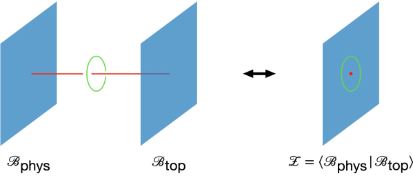
Figure 1: Absolute QFT as a SymTFT slab. The red line denotes an operator terminating on the gapped boundary $\mathcal{B}_{\text{top}}$, and the green line denotes an operator linking with it. After shrinking the slab, the resulting theory has a well-defined partition function $\mathcal{Z}$. The green loop is the symmetry operator measuring the charge of the heavy defect labeled by the red point.

From the operator algebra perspective, picking gapped boundary conditions corresponds to picking the Lagrangian subalgebra generated by a subset of operators in the SymTFT [59]. Generally speaking, TFT fields can pick the Dirichlet condition or the Neumann (i.e., free) condition at the gapped boundary. This will enable some topological operators to terminate on the topological boundary (red line in Figure 1) while others continue along the topological boundary (green loop in Figure 1 after pulling into the bulk). On the one hand, those continuing along the topological boundary are topological operators that generate the global symmetry for the absolute QFT. On the other hand, the Lagrangian subalgebra is generated by operators terminating on the gapped boundary with trivial linking and thus can be condensed simultaneously.

An illustrative example is the SymTFT for 4D $\mathfrak{su}(2)$ $\mathcal{N}=4$ super Yang-Mills (SYM) theory [14],

$$S_{5}=\frac{2\pi}{2}\int_{M_{5}}b_{2}\cup\delta c_{2},$$ (4)

where $b_{2}$ and $c_{2}$ are $\mathbb{Z}_{2}$-valued cochains, under the defect group $\mathbb{D}=\mathbb{Z}_{2}^{(e)}\times\mathbb{Z}_{2}^{(m)}$, respectively. The spectrum of surface topological operators for this 5D TFT reads

$$U_{(m,n)}(M_{2})=\exp\left(\pi i\int_{M_{2}}mb_{2}+nc_{2}\right),$$ (5)

where $m,n\in\{0,1\}$. Using the TFT quantization

$$\left[b_{ij}(x),c_{kl}(y)\right]=\frac{i}{\pi}\epsilon_{ijkl}\delta(x-y),$$ (6)

one obtains the non-trivial linking generated by

$$U_{(1,0)}(M_{2})U_{(0,1)}(M_{2}^{\prime})=U_{(0,1)}(M_{2}^{\prime})U_{(1,0)}(M_{2})e^{\pi i~{}\text{Link}(M_{2},M_{2}^{\prime})}.$$ (7)

On the physical boundary, local information (i.e., local operators and their correlation functions) of the SYM gives rise to the relative QFT with Lie algebra $\mathfrak{su}(2)$. The global form of the gauge group, however, is captured by the gapped boundary conditions on the topological boundary. For example, the gauge group $SU(2)$ is associated with the following boundary condition

$$b_{2}~{}\text{Dirichelt},c_{2}~{}\text{Neumann}.$$ (8)

The Lagrangian subalgebra corresponding to this boundary condition is generated by

$$\{U_{(0,0)},U_{(1,0)}\},$$ (9)

within which all operators have trivial linking, thus can be simultaneously condensed. This aligns with the fact that $U_{(0,0)}$ and $U_{(1,0)}$ can terminate on the gapped boundary because of the Dirichlet condition for $b_{2}$.

Lagrangian subgroups and polarization pairs

From the defect group perspective, a Lagrangian subalgebra associated with the gapped boundary conditions can be alternatively derived from a Lagrangian subgroup of the defect group: $L\subset\mathbb{D}$. The integral Dirac pairing of the sublattice required by a QFT with a well-defined partition function corresponds to the trivial linking between topological operators, which builds a Lagrangian subalgebra of the TFT.

The correspondence between the defect group and the SymTFT is discussed in detail in, e.g., [49, 58]. Briefly speaking, given an intermediate defect group in a $2k$-dimensional QFT with a generic form $\mathbb{D}=\oplus_{i}{\mathbb{Z}}_{N_{i}}$ and its corresponding Dirac pairing, one can write down a SymTFT with quadratic single-derivative action (namely Chern-Simons or BF-type terms),

$$S_{\text{symTFT}}[b_{i}]=\int_{M_{2k+1}}\frac{1}{2}b_{i}Q_{ij}\delta b_{j},$$ (10)

where $b_{i}$ is the background gauge field for ${\mathbb{Z}}_{N_{i}}\subset\mathbb{D}$, and the matrix $Q_{ij}$ is the coefficient of the $\mathbb{Q}/\mathbb{Z}$-valued bilinear Dirac pairing on the defect group $\mathbb{D}$ [49, 58]. A Lagrangian subgroup of the defect group with integral Dirac pairing is then translated into a gapped boundary condition of the SymTFT. This boundary condition then specifies a subset of $k$-dimensional topological operators in the SymTFT with trivial linking relations, generating a Lagrangian subalgebra.

Now, back to the 4D $\mathfrak{su}(2)$ SYM example, one can easily see the defect group is given by

$$\mathbb{D}=\mathbb{Z}_{2}^{(e)}\times\mathbb{Z}_{2}^{(m)},$$ (11)

whose background fields are $b_{2}$ and $c_{2}$, respectively. The defect group is equipped with an anti-symmetric Dirac pairing

$$\begin{pmatrix}0&\frac{1}{2}\\ -\frac{1}{2}&0\end{pmatrix}.$$ (12)

Denote elements in the defect group as $(a,b)\in\mathbb{D}$, where $a\in\mathbb{Z}_{2}^{(e)}$ and $b\in\mathbb{Z}_{2}^{(m)}$. The Lagrangian subgroup for the global form $SU(2)$ is given by

$$L_{SU(2)}=\mathbb{Z}_{2}^{(m)},$$ (13)

whose generating element $(0,1)$ enjoys integer Dirac pairing under (12). The 1-form global symmetry $G^{(1)}_{SU(2)}$ for the resulting absolute $SU(2)$ theory is then given by condensing the symmetry operators for $\mathbb{Z}_{2}^{(m)}$, namely treating it as the “gauged” part via the quotient

$$G^{(1)}_{SU(2)}=L^{\vee}_{SU(2)}\equiv\mathbb{D}/\mathbb{Z}_{2}^{(m)}$$ (14)

We remark that picking a gapped boundary condition/Lagrangian subalgebra may not fully fix the global structure of an absolute QFT. For example, after choosing the global form of the gauge group $SU(2)$, one can decide whether to further stack a $\mathbb{Z}_{2}$ symmetry-protected topological (SPT) phase $\exp\left(\frac{i\pi}{2}\int_{M_{4}}\mathcal{P}(b_{2})\right)$ to the theory, with $\mathcal{P}(b_{2})$ the Pontryagin square of $b_{2}$. Following the notation in [60], we denote the theory with and without SPT stacking as $SU(2)_{0}$ and $SU(2)_{1}$, respectively. These two theories, associated with the same Lagrangian subgroup, translate in two possible embeddings of $L^{\vee}$ in $\mathbb{D}$ as another Lagrangian subgroup $\overline{L}$

$$\begin{split}&L^{\vee}_{SU(2)}\rightarrow\overline{L}=\mathbb{Z}_{2}^{(e)},\\ \text{or}~{}&L^{\vee}_{SU(2)}\rightarrow\overline{L}=\mathbb{Z}_{2}^{(d)}\end{split}$$ (15)

so that

$$L\oplus\overline{L}=\mathbb{D},$$ (16)

where $\mathbb{Z}_{2}^{(d)}$ is the diagonal $\mathbb{Z}_{2}$ subgroup of $\mathbb{D}$.

The fully specified global structure of the theory is then given by a pair of Lagrangian subgroups $(L,\overline{L})$

$$\begin{split}&SU(2)_{0}:(L=\mathbb{Z}_{2}^{(m)},\overline{L}=\mathbb{Z}_{2}^{(e)}),\\ &SU(2)_{1}:(L=\mathbb{Z}_{2}^{(m)},\overline{L}=\mathbb{Z}_{2}^{(d)}),\end{split}$$ (17)

As we discussed previously in this section, this is a refined notion of polarization known as the polarization pair [49].

2.2 Relativeness: SymTFTs without Any Gapped Boundary Condition

It is not always possible to pick gapped boundary conditions for a given SymTFT. Alternatively speaking, SymTFTs exist whose spectrum of operators does not allow any Lagrangian subalgebra. In this case, one can only introduce a physical boundary for the SymTFT. The relative QFT living on the physical boundary does not admit any polarization/absolute QFT descendants. For the sake of clarity, we will refer to this type of QFT as intrinsically relative. Instead of a well-defined partition function in (3), the best one can do for this type of theory is to define a partition vector $|\mathcal{B}_{\text{phys}}\rangle$ in the Hilbert space from the quantization of the corresponding SymTFT.

An illustrative example is a $(4s+3)$-dimensional SymTFT such as a $U(1)_{2}$ Chern-Simons theory

$$S_{4s+3}=\frac{2}{4\pi}\int_{M_{4s+3}}c_{2s+1}\wedge dc_{2s+1},$$ (18)

where $c_{2s+1}$ is a $(2s+1)$-form $U(1)$ field. The topological operators of this theory are

$$U_{m}(M_{2s+1})=\exp\left(im\int_{M_{2s+1}}c_{2s+1}\right),m\in\mathbb{Z}_{2}$$ (19)

which, in the case of $s=0$, are just Wilson loops for 3D Chern-Simons Theory. Since we are just working in the case of Chern-Simons level $k=2$, there is only one non-trivial operator $U_{1}(M_{2s+1})$ with self-linking (see, e.g., [1])

$$U_{1}(M_{2s+1})U_{1}(M_{2s+1}^{\prime})=U_{1}(M_{2s+1}^{\prime})U_{1}(M_{2s+1})e^{\pi i~{}\text{Link}(M_{2s+1},M_{2s+1}^{\prime})}.$$ (20)

Therefore, there is no subset of operators with trivial linking, i.e., no Lagrangian subalgebra. This implies that there is no well-defined gapped boundary conditions for $c_{2s+1}$. This means on the physical boundary, the $(4s+2)$-dimensional QFT does not admit any polarization/absolute QFT descendent. In other words, its relativeness to the bulk SymTFT is inevitable.

No Lagrangian subgroup

This relativeness can also be seen from the perspective of the defect group. The defect group for the $(4s+2)$-dimensional QFT whose SymTFT is $U(1)_{2}$ Chern-Simons theory is given by a single factor

$$\mathbb{D}=\mathbb{Z}_{2}$$ (21)

with the symmetric Dirac pairing matrix, which in this case is just a $1\times 1$ matrix with a single element

$$\frac{1}{2}.$$ (22)

As discussed in the 4D $\mathfrak{su}(2)$ SYM case (13), one attempts to find a Lagrangian subgroup of the defect group associated with a possible well-defined gapped boundary condition. However, one necessary condition for a Lagrangian subgroup is

$$|L|^{2}=|\mathbb{D}|,$$ (23)

with $|G|$ the order of the group $G$. Therefore, $\mathbb{Z}_{2}$ has no Lagrangian subgroup; thus, this SymTFT does not admit a gapped boundary condition. That is to say, the associated $(4s+2)$ QFT is intrinsically relative.

When $s=0$, (18) is a 3D $U(1)_{2}$ Chern-Simons theory. One possible associated relative QFT is a 2D chiral CFT without modular-invariant partition function but with conformal blocks as the partition vector, e.g., the chiral WZW model. When $s=1$, (18) is equivalent to a 7D Chern-Simons theory for 3-form gauge field $c_{3}$. One possible class of the associated intrinsically relative QFTs includes 6D superconformal field theories (SCFTs) with the defect group $\mathbb{Z}_{2}$, e.g., $A_{1}$ $\mathcal{N}=(2,0)$ SCFT.

2.3 Anomalies: Obstructions to Certain Gapped Boundary Conditions

Generally speaking, there are two notions for defining the ’t Hooft anomalies of a global symmetry. One is defined as the obstruction of gauging the symmetry, while the other is defined as the obstruction to a symmetry-protected trivially gapped phase. For invertible symmetries, these two notions coincide, while for non-invertible symmetries, they can be non-equivalent [63]. In this work, we will use the former notion and translate the gauging obstruction as the obstruction to certain gapped boundary conditions for SymTFTs [37, 39, 36, 38].

2.3.1 Anomalous Invertible Symmetries

For invertible global symmetries, anomalies are nicely captured by $(D+1)$-dimensional invertible TFTs via the anomaly inflow construction [64]. The resulting invertible TFTs can then be embedded into SymTFTs by promoting all fields to be dynamical. For example, an anomalous $\mathbb{Z}_{2}$ symmetry with background field $A_{1}$ in 2D QFT can be described by a 3D term

$$\pi\int_{M_{3}}\frac{1}{2}A_{1}\cup\delta A_{1},$$ (24)

$\mathbb{Z}_{2}$ twisted Dijkgraaf-Witten theory

The anomaly term (24) can be embedded into a 3D SymTFT as a Dijkgraaf-Witten theory [65] by promoting $A_{1}$ into a dynamical field $a_{1}$ with a $H^{3}(U(1),\mathbb{Z}_{2})=\mathbb{Z}_{2}$ twist,

$$S_{3}=\frac{2\pi}{2}\int_{M_{3}}a_{1}\cup\delta\widehat{a}_{1}+\frac{2\pi}{4}\int_{M_{3}}a_{1}\cup\delta a_{1}.$$ (25)

Picking the gapped boundary condition

$$a_{1}~{}\text{Dirichlet},~{}\widehat{a}_{1}~{}\text{Neumann}$$ (26)

leads to a 2D absolute QFT with $\mathbb{Z}_{2}$ symmetry generated by $\exp\left(\pi i\int_{M_{1}}\widehat{a}_{1}\right)$ with anomalies (24). This “electric” boundary condition is allowed, since $\exp\left(\pi i\int_{M_{1}}a_{1}\right)$ has trivial self-linking such that

$$\{1,\exp\left(\pi i\int_{M_{1}}a_{1}\right)\}$$ (27)

generates a Lagrangian subalgebra.

An attempt to gauging the $\mathbb{Z}_{2}$ symmetry amounts to condensing the $\mathbb{Z}_{2}$ symmetry operator $\exp\left(\pi i\int_{M_{1}}\widehat{a}_{1}\right)$, leading to a naive “magnetic” boundary condition

$$a_{1}~{}\text{Neumann},~{}\widehat{a}_{1}~{}\text{Dirichlet}.$$ (28)

However, unlike the line operator for $a$, the topological line $\exp\left(\pi i\int_{M_{1}}\widehat{a}_{1}\right)$ has a non-trivial self-linking (see, e.g., [66])

$$\langle\exp\left(\pi i\int_{M_{1}}\widehat{a}_{1}\right)\exp\left(\pi i\int_{M_{1}^{\prime}}\widehat{a}_{1}\right)\rangle\sim e^{\pi i~{}\text{Link}(M_{1},M_{1}^{\prime})}.$$ (29)

This means it cannot generate a Lagrangian subalgebra and be condensed. Therefore, the “magnetic” boundary condition (28) is obstructed, capturing anomalies for the $\mathbb{Z}_{2}$ symmetry.

$U(1)_{4}$ Chern-Simons theory

In addition to the Dijkgraaf-Witten theory (25), another SymTFT able to realize the anomaly (24) is similar to the previous relativeness example (18), but this time a $U(1)_{4}$ Chern-Simons theory,

$$S_{3}=\frac{4}{4\pi}\int_{M_{3}}c_{1}\wedge dc_{1},$$ (30)

where $c_{1}$ is a 1-form $U(1)$ gauge field. The line operator spectrum of this theory is given by Wilson lines (19) with $m\in\mathbb{Z}_{4}$. The essential difference from the $U(1)_{2}$ case in (18) is now the operator $U_{2}(M_{1})$ has trivial self-linking. Therefore, it is possible to pick a Lagrangian subalgebra generated by

$$\{1,U_{2}(M_{1})\}$$ (31)

and define an associated gapped boundary condition

$$c_{1}|_{\partial M_{3}}=A_{1},$$ (32)

with $A_{1}$ a $\mathbb{Z}_{2}$-valued gauge field. This boundary condition leads to a 2D absolute QFT with a $\mathbb{Z}_{2}$ symmetry, whose anomaly is captured by (24).

This anomaly can be easily seen from the operator algebra perspective. Notice that (31) is the only possible Lagrangian subalgebra because all other line operators have non-trivial linkings. This obstruction to other boundary conditions by condensing topological operators implies the anomaly.

Anomaly as an obstruction to polarization pair

In the defect group language, the anomalies of $\mathbb{Z}_{2}$ symmetry can be interpreted as the obstruction to a polarization pair. Let us briefly discuss how this works for both the Dijkgraaf-Witten theory and the Chern-Simons theory as SymTFTs.

For the twisted Dijkgraaf-Witten theory (25), the associated 2D relative QFT has the defect group

$$\mathbb{D}=\mathbb{Z}_{2}^{(a)}\times\mathbb{Z}_{2}^{(\widehat{a})}$$ (33)

with a symmetric Dirac pairing matrix

$$\begin{pmatrix}\frac{1}{2}&\frac{1}{2}\\ \frac{1}{2}&0\end{pmatrix}.$$ (34)

The Lagrangian subgroup corresponding to the gapped boundary condition (26) is given by

$$L=\mathbb{Z}_{2}^{(\widehat{a})}\subset\mathbb{D}$$ (35)

generated by $(0,1)\in\mathbb{D}$, due to the integer Dirac pairing

$$(0,1)\begin{pmatrix}\frac{1}{2}&\frac{1}{2}\\ \frac{1}{2}&0\end{pmatrix}\begin{pmatrix}0\\ 1\end{pmatrix}\in\mathbb{Z}$$ (36)

It is straightforward to check all other non-trivial subgroups of $\mathbb{D}$ do not have integer Dirac pairing; thus, the global symmetry

$$L^{\vee}=\mathbb{D}/\mathbb{Z}_{2}^{(\widehat{a})}$$ (37)

cannot be uplifted to any Lagrangian subgroup. This obstructs the polarization associated with $L=\mathbb{Z}_{2}^{\widehat{a}}$ to be promoted into a polarization pair, which implies the global symmetry $L^{\vee}$ of the absolute QFT is anomalous.

For the $U(1)_{4}$ Chern-Simons theory, the associated 2D relative QFT has the defect group

$$\mathbb{D}=\mathbb{Z}_{4}$$ (38)

with a single $1\times 1$ matrix element $\frac{1}{4}$ as the symmetric Dirac pairing. The Lagrangian subgroup corresponding to the gapped boundary condition (32) is given by

$$L=\mathbb{Z}_{2}\subset\mathbb{D},$$ (39)

due to the integer Dirac pairing $\frac{1}{4}\times 2^{2}\in\mathbb{Z}$. The global symmetry $\mathbb{Z}_{2}=L^{\vee}\equiv\mathbb{D}/\mathbb{Z}_{2}$ of the resulting absolute theory cannot be embedded back in $\mathbb{D}=\mathbb{Z}_{4}$ as a Lagrangian subgroup. This is due to the fact that the short exact sequence

$$1\rightarrow L={\mathbb{Z}}_{2}\rightarrow{\mathbb{Z}}_{4}\rightarrow L^{\vee}={\mathbb{Z}}_{2}\rightarrow 1$$ (40)

does not split. This obstructs the polarization associated with $L=\mathbb{Z}_{2}$ to be promoted as a polarization pair, which implies the anomaly of the $\mathbb{Z}_{2}$ symmetry.

2.3.2 Anomalous Non-invertible Symmetries

The anomalies of non-invertible symmetries can be captured following the same philosophy as those of invertible symmetries. Namely, starting with a polarization/gapped boundary condition, referred to as “electric”, whose corresponding absolute QFT enjoys a non-invertible symmetry, the obstruction to its “magnetic” boundary condition via simultaneously condensing topological operators implies the anomaly for the non-invertible symmetry [37, 39, 38].

An illustrative example is discussed in [37], where the authors constructed an anomalous non-invertible symmetry given by the $\mathbb{Z}_{2}\times\mathbb{Z}_{2}$ Tambara-Yamagami (TY) fusion category [67]. Here, we briefly review their result. Consider a 2D QFT enjoying a $\mathbb{Z}_{2}^{(a)}\times\mathbb{Z}_{2}^{(b)}\times\mathbb{Z}_{2}^{(c)}$ symmetry with anomalies captured by a 3D invertible TFT

$$\pi\int_{M_{3}}\frac{1}{2}A_{1}\cup\delta A_{1}+A_{1}\cup B_{1}\cup C_{1},$$ (41)

where $A_{1},B_{1}$ and $C_{1}$ are ${\mathbb{Z}}_{2}$ cochains as background fields for ${\mathbb{Z}}_{2}^{(a)},{\mathbb{Z}}_{2}^{(b)}$ and ${\mathbb{Z}}_{2}^{(c)}$, respectively. Gauging the ${\mathbb{Z}}_{2}^{(b)}\times{\mathbb{Z}}_{2}^{(c)}$ symmetry, the topological line operator $L(M_{1};a)$ for ${\mathbb{Z}}_{2}^{(a)}$ then fails to be gauge-invariant, but can be cured by stacking a 1D ${\mathbb{Z}}_{2}\times{\mathbb{Z}}_{2}$ Dijkgraaf-Witten theory [37, 52]

$$\mathcal{N}(M_{1};b_{1},c_{1})\equiv L(M_{1};b_{1},c_{1})\int{\mathcal{D}}\widehat{\phi}_{0}\mathcal{D}\phi_{0}\exp\left(\pi i\int_{M_{1}}\widehat{\phi}_{0}\cup\delta\phi_{0}+\phi_{0}\cup b_{1}-\widehat{\phi}_{0}\cup c_{1}\right),$$ (42)

where $\phi_{0}$ and $\widehat{\phi}_{0}$ $\mathbb{Z}_{2}$-valued 0-cochains and $b_{1},c_{1}$ are dynamical fields from promoting $B_{1},C_{1}$ via gauging. This non-invertible defect line generates a ${\mathbb{Z}}_{2}\times{\mathbb{Z}}_{2}$ Tambara-Yamagami (TY) fusion categorical symmetry [67], which we will denote as TY$({\mathbb{Z}}_{2}\times{\mathbb{Z}}_{2})$.

Note that this categorical symmetry is inherited from the invertible symmetry ${\mathbb{Z}}_{2}^{a}$. Its anomaly can then be regarded as also inherited from the self-anomaly given by the first term in (51). More specifically, one can consider embedding this anomaly TFT into a SymTFT

$$S_{3}=\frac{2\pi}{2}\int_{M_{3}}a_{1}\cup\delta\widehat{a}_{1}+b_{1}\cup\delta\widehat{b}_{1}+c_{1}\cup\delta\widehat{c}_{1}+\frac{1}{2}a_{1}\cup\delta a_{1}+a_{1}\cup b_{1}\cup c_{1}.$$ (43)

The absolute QFT enjoying the TY$({\mathbb{Z}}_{2}\times{\mathbb{Z}}_{2})$ categorical symmetry is given by the following “electric” gapped boundary condition

$$a_{1},\widehat{b}_{1},\widehat{c}_{1}~{}\text{Dirichlet},~{}\widehat{a}_{1},b_{1},c_{1}~{}\text{Neumann}$$ (44)

under which the topological line operator

$$L_{\widehat{a}_{1},b_{1},c_{1}}(M_{1})=\int{\mathcal{D}}\widehat{\phi}_{0}{\mathcal{D}}\phi_{0}\exp\left(\pi i\int_{M_{1}}\widehat{a}_{1}\right)\exp\left(\pi i\int_{M_{1}}\widehat{\phi}_{0}\cup\delta\phi_{0}+\phi_{0}\cup b_{1}-\widehat{\phi}_{0}\cup c_{1}\right)$$ (45)

corresponds to the symmetry generator $\mathcal{N}(M_{1};b_{1},c_{1})$ (42). It is computed in [37] that there is always a non-trivial linking for $L_{\widehat{a}_{1},b_{1},c_{1}}(M_{1})$

$$\langle L_{\widehat{a}_{1},b_{1},c_{1}}(M_{1})L_{\widehat{a}_{1},b_{1},c_{1}}(M_{1}^{\prime})\rangle\sim e^{\pi i~{}\text{Link}(M_{1},M_{1}^{\prime})}\neq 1,$$ (46)

due to the term $\frac{1}{2}a_{1}\cup\delta a_{1}$ in the SymTFT. This non-trivial linking prevents the operator $L_{\widehat{a}_{1},b_{1},c_{1}}(M_{1})$ from forming any Lagrangian subalgebra, implying the obstruction to the “magnetic” gapped boundary condition on which the $L_{\widehat{a}_{1},b_{1},c_{1}}(M_{1})$ line can terminate.

Anomaly from obstruction to polarization pair

Let us try understanding this anomaly for non-invertible symmetries from the defect group and the polarization pair perspective. The single-derivative terms in SymTFT (43) show that the associated 2D relative QFT has the defect group

$$\mathbb{D}={\mathbb{Z}}_{2}^{(a)}\times{\mathbb{Z}}_{2}^{(\widehat{a})}\times{\mathbb{Z}}_{2}^{(b)}\times{\mathbb{Z}}_{2}^{(\widehat{b})}\times{\mathbb{Z}}_{2}^{(c)}\times{\mathbb{Z}}_{2}^{(\widehat{c})},$$ (47)

with the Dirac pairing matrix

$$\begin{pmatrix}{\color[rgb]{1,0,0}\frac{1}{2}}&\frac{1}{2}&0&0&0&0\\ \frac{1}{2}&0&0&0&0&0\\ 0&0&0&\frac{1}{2}&0&0\\ 0&0&\frac{1}{2}&0&0&0\\ 0&0&0&0&0&\frac{1}{2}\\ 0&0&0&0&\frac{1}{2}&0\\ \end{pmatrix}.$$ (48)

This defect group admits many Lagrangian subgroups with integral Dirac pairing under (48). One of them is $L_{1}={\mathbb{Z}}_{2}^{(\widehat{a})}\times{\mathbb{Z}}_{2}^{(\widehat{b})}\times{\mathbb{Z}}_{2}^{(\widehat{c})}$, corresponding to an absolute 2D QFT with global symmetry,

$$L^{\vee}_{1}=\mathbb{D}/L_{1}\cong{\mathbb{Z}}_{2}^{(a)}\times{\mathbb{Z}}_{2}^{(b)}\times{\mathbb{Z}}_{2}^{(c)},$$ (49)

with the anomaly TFT as shown previously in (51). One might try promoting this polarization $L_{1}$ into a polarization pair, but will then find out the ${\mathbb{Z}}_{2}^{(a)}\times{\mathbb{Z}}_{2}^{(b)}\times{\mathbb{Z}}_{2}^{(c)}$ does not enjoy a integral Dirac pairing under (48). This means $L_{1}^{\vee}$ cannot be embedded into $\mathbb{D}$ as a Lagrangian subgroup, which implies the obstruction to gauging the full $L_{1}^{\vee}$ symmetry.

However, it is possible to gauge part of the $L_{1}^{\vee}$, namely the ${\mathbb{Z}}_{2}^{(b)}\times{\mathbb{Z}}_{2}^{(c)}$ symmetry. The resulting polarization is given by flipping the role of $b,c$ with $\widehat{b},\widehat{c}$, resulting in the Lagrangian subgroup $L_{2}={\mathbb{Z}}_{2}^{(\widehat{a})}\times{\mathbb{Z}}_{2}^{(b)}\times{\mathbb{Z}}_{2}^{(c)}$. The associated quotient $L_{2}^{\vee}$ of the defect group reads

$$L_{2}^{\vee}=\mathbb{D}/L_{2}\cong{\mathbb{Z}}_{2}^{(a)}\times{\mathbb{Z}}_{2}^{(\widehat{b})}\times{\mathbb{Z}}_{2}^{(\widehat{c})}.$$ (50)

However, in the presence of the cubic term in $(\ref{eq: symtft for anomalous noninver})$, $L^{\vee}_{2}$ is not the genuine global symmetry for the absolute QFT, but it is promoted to a non-invertible symmetry.

$$L^{\vee}_{2}\rightarrow G=\text{TY}({\mathbb{Z}}_{2}\times{\mathbb{Z}}_{2})$$ (51)

This promotion can be understood as replacing the direct product in $L^{\vee}_{2}$ between ${\mathbb{Z}}_{2}^{(a)}$ and ${\mathbb{Z}}_{2}^{(\widehat{b})}\times{\mathbb{Z}}_{2}^{(\widehat{c})}$ with a ${\mathbb{Z}}_{2}^{(a)}$ extension of the invertible fusion category Vec$({\mathbb{Z}}_{2}^{(\widehat{b})}\times{\mathbb{Z}}_{2}^{(\widehat{c})})$. The result of this non-trivial group extension is exactly the TY$({\mathbb{Z}}_{2}\times{\mathbb{Z}}_{2})$ non-invertible symmetry.

Now it is also straightforward to see why this non-invertible symmetry is anomalous. An attempt to gauge this non-invertible symmetry translates in promoting $L_{2}^{\vee}$ into a Lagrangian subgroup in order to build a polarization pair refined from the $L_{2}$ polarization. However, one can check that ${\mathbb{Z}}_{2}^{(a)}\times{\mathbb{Z}}_{2}^{(\widehat{b})}\times{\mathbb{Z}}_{2}^{(\widehat{c})}$ does not enjoy a integral Dirac pairing, due to the $\frac{1}{2}$ element labeled in red in the pairing matrix (48). Therefore, $L_{2}^{\vee}$ cannot be uplifted to a Lagrangian subgroup of $\mathbb{D}$, implying the anomaly which the descendent global symmetry $G=$TY$({\mathbb{Z}}_{2}\times{\mathbb{Z}}_{2})$ suffers from. Note that the $\frac{1}{2}$ in red in (48) is exactly the coefficient responsible for the self-anomaly term $\frac{1}{2}A_{1}\cup\delta A_{1}$ in (51), which we have argued from the SymTFT gapped boundary condition point of view, is the origin of the anomaly for the non-invertible symmetry.

3 2D QFTs from Calabi-Yau 4-Folds

In this paper, we will focus on 2D $(0,2)$ gauge theories engineered on D1-branes probing toric Calabi-Yau 4-folds. These theories can be efficiently encoded in terms of brane brick models, which are obtained from D1-branes at Calabi-Yau 4-fold singularities by T-duality. We refer the reader to [71, 72, 73, 74] for detailed discussions.

A brane brick model is a Type IIA brane configuration consisting of D4-branes wrapping a 3-torus $\mathbb{T}^{3}$ and suspended from an NS5-brane that wraps a holomorphic surface $\Sigma$ intersecting with $\mathbb{T}^{3}$. The holomorphic surface $\Sigma$ is the zero locus of the Newton polynomial defined by the toric diagram of the Calabi-Yau 4-fold. As an example, Figure 2 shows the brane brick model for $\mathbb{C}^{4}$. The corresponding QFT is the $(8,8)$ theory obtained from dimensionally reducing 4D $\mathcal{N}=4$ SYM to 2D.

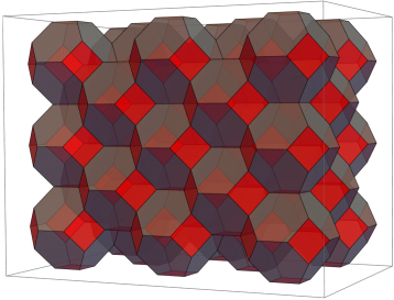
Figure 2: Brane brick model for $\mathbb{C}^{4}$. Here we show multiple copies of the unit cell.

Table 1 summarizes the basic ingredients in a Brane Brick Model. The $(246)$ directions are compactified on a 3-torus, while the 2D gauge theory lives on the $(01)$ directions common to all the branes.

	0	1	2	3	4	5	6	7	8	9
D4	$\times$	$\times$	$\times$	$\cdot$	$\times$	$\cdot$	$\times$	$\cdot$	$\cdot$	$\cdot$
NS5	$\times$	$\times$	———–  $\Sigma$  ————						$\cdot$	$\cdot$

Table 1: Brane brick model configuration.

Brane brick models, or equivalently their dual periodic quivers, fully specify the 2D $(0,2)$ quiver gauge theories on the worldvolume of D1-branes probing toric Calabi-Yau 4-folds. The dictionary connecting brane brick models to the corresponding gauge theories is summarized in Table 2.

Brane Brick Model	Gauge Theory	Periodic Quiver
Brick	Gauge group	Node
Oriented face	Bifundamental chiral field from	Oriented (black) arrow
between bricks $i$ and $j$	node $i$ to node $j$ (adjoint if $i=j$)	from node $i$ to node $j$
Unoriented square face	Bifundamental Fermi field between	Unoriented (red) line
between bricks $i$ and $j$	nodes $i$ and $j$ (adjoint if $i=j$)	between nodes $i$ and $j$
Edge	$J$- or $E$-term	Plaquette encoding
		a $J$- or an $E$-term

Table 2: Dictionary between brane brick models and $2d$ $(0,2)$ gauge theories.

Brane brick models streamline the connection between gauge theory and the underlying geometry (see, e.g., [72, 74, 75, 76]). Additional results on brane brick models can be found in [77, 78, 79].

4 Aspects of Generalized Symmetries in 2D from String Theory

Having reviewed how 2D QFTs can be engineered from Calabi-Yau 4-folds in Type IIB string theory, in this section, we discuss how to extract categorical symmetries for this infinite class of theories from the geometric data. In particular, we will present a general prescription for deriving 3D SymTFTs via dimensional reduction of the topological sector of type IIB supergravity. Furthermore, we also discuss how the topological operators in the 3D SymTFTs can be derived from the brane worldvolume actions via the construction of branes “at infinity”. The gapped boundary conditions are translated into boundary conditions for various IIB fluxes “at infinity”, under which the dimensionally reduced brane worldvolume actions serve as charged objects generating the Lagrangian subalgebra and symmetry operators for the associated absolute 2D QFTs.

4.1 3D Symmetry TFTs from Type IIB string theory

Consider 2D QFTs associated with singular Calabi-Yau 4-folds $Y$, whose base spaces are Sasaki-Einstein 7-manifold, probed by D1-branes. The IIB string theory background reads

$$M_{2}\times Y\rightarrow M_{3}\times\partial Y$$ (52)

where $M_{2}$ is the 2D spacetime where the D1-branes worldvolume extending, living on the boundary of a 3D bulk manifold $M_{3}=M_{2}\times\mathbb{R}_{\geq 0}$. The asymptotic boundary $\partial Y$ is given by the Sasaki-Einstein base space of $Y$.

To compute a SymTFT supported on $M_{3}$, we ought to dimensionally reduce the topological sector of IIB string theory on $\partial Y$. The relevant topological action involves various IIB fluxes, among which we are interested in $F_{5}$, $G_{3}$, and $H_{3}$ which are electrically (resp. magnetically) sourced by D3 (resp. D3), D1 (resp. D5), and F1 (resp. NS5)-branes, respectively. Technically, the dimensional reduction starts from treating the various IIB supergravity fluxes as elements in differential cohomology classes $\breve{H}^{*}(\partial Y)$ (see, e.g., [80, 81, 57]) sitting in the exact sequences

$$0~{}\rightarrow~{}H^{p-1}(\partial Y;{\mathbb{R}}/{\mathbb{Z}})~{}\rightarrow~{}\breve{H}^{p}(\partial Y)~{}\rightarrow~{}\Omega_{\mathbb{Z}}^{p}(\partial Y)~{}\rightarrow~{}0$$ (53)

and

$$0~{}\rightarrow~{}\Omega^{p-1}(\partial Y)/\Omega^{p-1}_{{\mathbb{Z}}}(\partial Y)~{}\rightarrow~{}\breve{H}^{p}(\partial Y)~{}\stackrel{{\scriptstyle\pi}}{{\rightarrow}}~{}H^{p}(\partial Y;{\mathbb{Z}})~{}\rightarrow~{}0$$ (54)

where $\Omega^{p-1}(\partial Y)$ (resp. $\Omega^{p-1}_{{\mathbb{Z}}}(\partial Y)$) denotes closed differential $p$-forms (resp. with integral periods). To be explicit, we assume the following cohomology classes for $\partial Y$:

$$H^{*}(\partial Y;\mathbb{Z})=\left\{\mathbb{Z},0,\mathbb{Z}^{b_{2}}\oplus\Gamma_{2},0,\Gamma_{4},\mathbb{Z}^{b_{5}},\Gamma_{6},\mathbb{Z}\right\},$$ (55)

which covers an infinite family of Calabi-Yau 4-fold singularities, including orbifolds ${\mathbb{C}}^{4}/\Gamma$ with isolated singularities, as well as cones over $Y^{p,k}(B_{4})$ with base space $B_{4}=\mathbb{P}^{1}\times\mathbb{P}^{1}$ or $B_{4}=\mathbb{P}^{2}$ [82]. In the above cohomology classes, $b_{2}$ and $b_{5}$ are, respectively, the second and the fifth Betti numbers, and $\Gamma_{n}$ is the torsional part of the $n$-th cohomology class. In particular, we have $b_{2}=b_{5}$ and $\Gamma_{6}=\Gamma_{2}$ due to Poincaré duality and universal coefficient theorem [83].

Due to the self-duality of the 5-form field strength $F_{5}$, a consistent way to capture the relevant terms in IIB supergravity action is to write down a topological action defined on an auxiliary 11D manifold $M_{11}$ (see, e.g., [86, 87, 35, 57, 88, 89, 90, 44, 49, 52])

$$\frac{S_{11}}{2\pi}=\int_{M_{11}}\frac{1}{2}F_{5}\wedge dF_{5}-F_{5}\wedge H_{3}\wedge G_{3}$$ (56)

and then perform the cohomology uplift [81, 49, 52, 35]

$$\frac{S_{11}}{2\pi}\rightarrow\int_{M_{11}}\frac{1}{2}\breve{F}_{6}\star\breve{F}_{6}-\breve{F}_{6}\star\breve{H_{3}}\star\breve{G}_{3}.$$ (57)

In the above expression, IIB fluxes are uplifted into differential cohomology elements

$$\breve{F}_{6}\in\breve{H}^{6}(M_{11}),\breve{H}_{3}\in\breve{H}^{3}(M_{11}),\breve{G}_{3}\in\breve{H}^{3}(M_{11}),$$ (58)

and the $\star$ symbol defines a bilinear product operation on Cheeger–Simons characters $\breve{H}^{k_{1}}(M_{d})\times\breve{H}^{k_{2}}(M_{d})=\breve{H}^{k_{1}+k_{2}}(M_{d})$ [91, 92]. In particular, the integral in the second line of (57) describes a perfect pairing $\breve{H}^{k_{1}}(M_{d})\times\breve{H}^{d+1-k_{1}}(M_{d})\rightarrow\mathbb{R}/\mathbb{Z}$. The case of our interest is $M_{11}=N_{4}\times\partial Y$, where the auxiliary 4-manifold $N_{4}$ has the boundary $\partial N_{4}=M_{3}$ supporting the SymTFT to be derived. Under this decomposition of $M_{11}$, we can expand the $\breve{F}_{6},\breve{H}_{3}$ and $\breve{G}_{3}$ based on (55)

$$\begin{split}\breve{F}_{6}=&\sum_{j}\breve{a}_{4}^{(j)}\star\breve{t}_{2(j)}+\sum_{i}\breve{a}_{2}^{(i)}\star\breve{t}_{4(i)}+\cdots,\\ \breve{H}_{3}=&\sum_{j}\breve{b}_{1}^{(j)}\star\breve{t}_{2(j)}+\cdots,\\ \breve{G}_{3}=&\sum_{j}\breve{c}_{1}^{(j)}\star\breve{t}_{2(j)}+\cdots,\end{split}$$ (59)

where $\breve{t}_{2(j)}$ and $\breve{t}_{4(i)}$ are generators respectively corresponding to $\Gamma_{2}$ and $\Gamma_{4}$, with indices $j$ and $i$ run over the generators. In the above expansion (59), we only make the torsional part explicit while suppressing the non-torsional part in “$\cdots$”. This is because we only focus on finite symmetries in this work. We defer the investigation of the non-torsional part and its associated continuous symmetries to future work.

Performing the dimensional reduction via integrating over $\partial Y$, we arrive at a 4D action

$$\begin{split}\frac{S_{4}}{2\pi}&=\int_{N_{4}}\frac{1}{2}\sum_{i_{1},i_{2}}\Lambda_{i_{1}i_{2}}\breve{a}_{2}^{(i_{1})}\star\breve{a}_{2}^{(i_{2})}+\sum_{i,j_{1},j_{2}}\Delta_{ij_{1}j_{2}}\breve{a}_{2}^{(i)}\star\breve{b}_{1}^{(j_{1})}\star\breve{c}_{1}^{(j_{2})},\\ \end{split}$$ (60)

where $\Lambda_{i_{1}i_{2}}$ and $\Delta_{ij_{2}j_{2}}$ are linking numbers defined by

$$\begin{split}\Lambda_{i_{1}i_{2}}&\equiv\int_{\partial Y}\breve{t}_{4(i_{1})}\star\breve{t}_{4(i_{2})}~{}\text{mod 1},\\ \Delta_{ij_{1}j_{2}}&\equiv-\int_{\partial Y}\breve{t}_{4(i)}\star\breve{t}_{2(j_{1})}\star\breve{t}_{2(j_{2})}~{}\text{mod 1}.\end{split}$$ (61)

These linking numbers can be derived from intersection numbers between divisors of the Calabi-Yau 4-fold $Y$ [51, 52]. We further assume $M_{3}=\partial N_{4}$ satisfying $H^{2}(M_{3},\mathbb{Z})=0$ so that $\breve{a}_{2}$ supported on $N_{4}$ can be trivialized to $\breve{a}_{1}$ on $M_{3}$ [35]. This allows us to write down a 3D action in terms of ordinary cochains

$$\frac{S_{3}}{2\pi}=\int_{M_{3}}\frac{1}{2}\Lambda_{i_{1}i_{2}}a_{1}^{(i_{1})}\cup\delta a_{1}^{(i_{2})}+\sum_{i,j_{1},j_{2}}\Delta_{ij_{1}j_{2}}a_{1}^{(i)}\cup b_{1}^{(j_{1})}\cup c_{1}^{(j_{2})}.$$ (62)

It is easy to see from (62) that there are three classes of 0-form finite symmetries $\Gamma^{(a^{(i)})},\Gamma^{(b^{(j)})}$ and $\Gamma^{(c^{(j)})}$, with background fields $a^{(i)},b^{(j)}$ and $c^{(j)}$, respectively. The geometric counterparts of these three symmetries are

$$\Gamma^{(a^{(i)})}=\Gamma_{4}^{(i)},~{}\Gamma^{(b^{(j)})}=\Gamma_{2}^{(j)},~{}\Gamma^{(c^{(j)})}=\Gamma_{2}^{(j)},$$ (63)

where $\Gamma_{2}=\oplus_{i}\Gamma^{(i)}_{2}$ and $\Gamma_{4}=\oplus_{j}\Gamma^{(j)}_{4}$ are torsional cohomology generators of $H^{*}(\partial Y;{\mathbb{Z}})$ in (55). However, the action (62) is incomplete. This can be seen by noticing that for $\Gamma^{(a^{(i)})}$ symmetries, the first term in (62) encodes the dual quantum symmetry information (if possible gauging is allowed) since it is single-derivative in the form of Dijkgraaf-Witten/Chern-Simons. Similarly, we need the information about the possible gauging of $\Gamma^{(b^{(j)})}$ and $\Gamma^{(c^{(j)})}$ and the dual quantum symmetries, for which the single-derivative terms are missing in (62).

According to [52] (see also, e.g., [50, 26] for a similar discussion in higher-dimensional setups), these extra terms for $\Gamma^{(b^{(j)})}$ and $\Gamma^{(c^{(j)})}$ symmetries can be added by the following argument. Notice that the first term in (62) is single-derivative and comes from the linking between the following two wrapped D3-branes

$$\text{D3-brane on $\gamma_{3}^{(i_{1})}$, D3-brane on $\gamma_{3}^{(i_{2})}$},$$ (64)

where $\gamma_{3}^{(i_{1})}$ and $\gamma_{3}^{(i_{2})}$ are torsional 3-cycles dual to two generators of the cohomology class $\text{Tor}{H}^{4}(\partial Y;{\mathbb{Z}})=\Gamma_{4}$. The corresponding differential cohomology generators are $\breve{t}_{4(i_{1})}$ and $\breve{t}_{4(i_{1})}$. The linking invariant between these two torsional 3-cycles is encoded in the first linking pairing in (61). Similarly, one can consider the linking pairs between the following wrapped branes

$$\begin{split}&\text{F1-string on $\gamma_{1}^{(j_{1})}$, NS5-brane on $\gamma_{5(j_{2})}$},\\ &\text{D1-string on $\gamma_{1}^{(j_{1})}$, D5-brane on $\gamma_{5(j_{2})}$},\end{split}$$ (65)

where $\gamma_{1}^{(j_{1})}$ and $\gamma_{5(j_{2})}$ are torsional 1-cycle and 5-cycle dual to the cohomology class $\text{Tor}H^{2}(\partial Y,{\mathbb{Z}})=\Gamma_{2}$ and $\text{Tor}H^{6}(\partial Y,{\mathbb{Z}})=\Gamma_{6}$, respectively. The linking invariant between these two torsional cycles can be computed via the differential cohomology pairing

$$\Omega_{j_{1}}^{j_{2}}\equiv\int_{\partial Y}\breve{t}_{2(j_{1})}\star\breve{t}_{6}^{(j_{2})}~{}\text{mod}~{}1,$$ (66)

where $\breve{t}_{6}^{(j_{2})}$ is the $j_{2}$-th generator of $\breve{H}^{6}(\partial Y)$ associated to $\Gamma_{6}=\oplus_{j}\Gamma_{6(j)}$. These give rise to two more classes of 0-form finite symmetries

$$\Gamma^{(\widehat{b}_{(j)})}=\Gamma_{6(j)},~{}\Gamma^{(\widehat{c}_{(j)})}=\Gamma_{6(j)}$$ (67)

whose background fields are $\widehat{b}_{(j)}$ and $\widehat{c}_{(j)}$, corresponding to correspond to NS5 and D5-branes in (65) respectively, in obvious notations.

Adding the extra terms from the pairing (65) and (66), we end up with the 3D SymTFT action

$$\boxed{\begin{split}S_{3}=&2\pi\int_{M_{3}}\frac{1}{2}\Lambda_{i_{1}i_{2}}a_{1}^{(i_{1})}\cup\delta a_{1}^{(i_{2})}+\Omega_{j_{1}}^{j_{2}}b_{1}^{(j_{1})}\cup\widehat{b}_{1(j_{2})}-\Omega_{j_{1}}^{j_{2}}c_{1}^{(j_{1})}\cup\widehat{c}_{1(j_{2})}+\\ &+\sum_{i,j_{1},j_{2}}\Delta_{ij_{1}j_{2}}a_{1}^{(i)}\cup b_{1}^{(j_{1})}\cup c_{1}^{(j_{2})}.\end{split}}$$ (68)

Before investigating this general SymTFT, we remark that though in this work, we derive the single-derivative terms in (68) from the flux non-commutativity and the associated brane linking in (64) and (65), there is an alternative way to derive these terms via dimensionally reducing the kinetic terms directly in 10D IIB supergravity action in terms of the non-harmonic differential forms (see e.g., [26, 95]).

4.1.1 Defect Group and Relativeness

Let us start with the defect group. The defect group for the SymTFT (68) can be read from (63) and (67)

$$\begin{split}\mathbb{D}&=\prod_{i}\Gamma^{(a^{(i)})}\times\prod_{j}\left(\Gamma^{(b^{(j)})}\times\Gamma^{(\widehat{b}_{(j)})}\right)\times\prod_{j}\left(\Gamma^{(c^{(j)})}\times\Gamma^{(\widehat{c}_{(j)})}\right)\\ &=\Gamma_{4}\times(\Gamma_{2}\times\Gamma_{6})\times(\Gamma_{2}\times\Gamma_{6}),\end{split}$$ (69)

where the $\Gamma$’s are given by the geometric data (55). Using the condition $\Gamma_{2}=\Gamma_{6}$ below (55), we obtain the defect group

$$\mathbb{D}=\Gamma_{4}\times(\Gamma_{2}^{(b)}\times\Gamma_{2}^{(\widehat{b})})\times(\Gamma_{2}^{(c)}\times\Gamma_{2}^{(\widehat{c})}),$$ (70)

where we use indices to distinguish various $\Gamma_{2}$ factors.

The Dirac pairing for the defect group, as we discussed around (10), is given by the single-derivative terms in the SymTFT, i.e., the first line in (68). It is easy to see that for the $\Gamma_{2}$ part of the defect group, there always exist Lagrangian subgroups in the form of

$$\Gamma_{2}\times\Gamma_{2}\subset(\Gamma_{2}^{(b)}\times\Gamma_{2}^{(\widehat{b})})\times(\Gamma_{2}^{(c)}\times\Gamma_{2}^{(\widehat{c})}),$$ (71)

associated with purely “electric” or “magnetic” gapped boundary conditions. For example, the subgroup $\Gamma_{2}^{(\widehat{b})}\times\Gamma_{2}^{(\widehat{c})}$ corresponds to the gapped boundary condition

$$b^{(j)}~{}\text{and}~{}c^{(j)}~{}\text{Dirichlet},~{}\widehat{b}_{(j)}~{}\text{and}~{}\widehat{c}_{(j)}~{}\text{Neumann}$$ (72)

for all $j$. This matches the fact that for this part of the defect group, the Dirac pairing is anti-symmetric, analogous to the $\mathfrak{su}(2)$ SYM example in Section 2.1.

However, the $\Gamma_{4}$ part in the defect group is not guaranteed to have a Lagrangian subgroup. Recall one necessary condition for a Lagrangian subgroup is (23), which means only if the $|\Gamma_{4}|=m^{2},m\in{\mathbb{Z}}$ can a Lagrangian subgroup of $\Gamma_{4}$ possibly exist. In other words, if $|\Gamma_{4}|$ is not a complete square, then there is no well-defined gapped boundary condition that can be picked for $a^{(i)}$ fields. Intuitively, this can be understood since the single-derivative terms for $a^{(i)}$ in the SymTFT (68) may just include Chern-Simons-type terms similar to (18) where no gapped boundary condition can be defined. According to the discussion in Section 2.2, in these cases, the associated 2D QFTs are intrinsically relative. Therefore, we end up with the following statement:

A sufficient condition for relativeness:

Let $\mathcal{T}$ be a 2D QFT engineered from a Calabi-Yau 4-fold $Y$ probed by D1-branes. Then $\mathcal{T}$ is an intrinsically relative QFT if $|\text{Tor}H^{4}(\partial Y;{\mathbb{Z}})|$ is not a complete square.

This relativeness for 2D QFTs is reminiscent of an infinite class of 6D SCFTs as relative theories [96, 97, 58, 49]. In fact, the relativeness of 6D SCFTs and our interested 2D QFTs enjoy a related string theory origin, namely the flux-noncommutativity for the self-dual $F_{5}$ flux in IIB string theory. After dimensional reduction to the topological sector of IIB compactification, this flux-noncommutativity leads to the obstruction of a well-defined boundary condition “at infinity” for lower-dimensional fields inherited from $F_{5}$. In the SymTFT language, this translates into the self-linking of the operators built on D3-branes and, as a result, prevents any Lagrangian subalgebra/gapped boundary condition. We will illustrate this top-down approach to the 2D relativeness with an explicit example in Section 5.

4.1.2 Non-invertible Symmetries and their Anomalies

After discussing the case when 2D QFTs are intrinsically relative, let us now consider the case when Calabi-Yau 4-folds $Y$ with the order of $\Gamma_{4}=\text{Tor}H^{4}(\partial Y;{\mathbb{Z}})$ a complete square, and further assume the SymTFT (68) admits gapped boundary conditions. We can split the $\Gamma_{4}$ generators as

$$\Gamma_{4}=\oplus_{i}\Gamma_{4}^{(i)}=\oplus_{k}\Gamma_{4}^{(k)}\oplus_{l}\Gamma_{4}^{(l)},$$ (73)

and then, without loss of generality, assume a standard “electric” gapped boundary condition, picking a Dirichlet condition for the following fields

$$a_{1}^{(k)},b_{1}^{(j)},c_{1}^{(j)}~{}\text{Dirichlet},$$ (74)

The resulting absolute QFT enjoys three classes of invertible finite symmetries

$$G^{(a^{(k)})}=\Gamma_{4}^{(k)},~{}G^{(b^{(j)})}=\Gamma_{2}^{(j)},~{}G^{(c^{(j)})}=\Gamma_{2}^{(j)},$$ (75)

whose respective background gauge fields are those given in (74).

For these three classes of invertible symmetries, there are mixed anomalies from the relevant cubic terms in the SymTFT (68)

$$\int_{M_{3}}\sum_{k,j_{1},j_{2}}\Delta_{kj_{1}j_{2}}a_{1}^{(k)}\cup b_{1}^{(j_{1})}\cup c_{1}^{(j_{2})}.$$ (76)

According to [98], which we also reviewed in Section 2.3, gauging two of the three classes of symmetries will promote the leftover one to non-invertible symmetries. In fact, based on our discussion around (71), it is always possible to gauge the $G^{(b^{(j)})}$ and $G^{(c^{(j)})}$ symmetry and end up with a “magnetic” boundary condition

$$a_{1}^{(k)},\widehat{b}_{1(j)},\widehat{c}_{1(j)}~{}\text{Dirichlet}.$$ (77)

The resulting absolute QFT under this condition has two classes of invertible symmetries

$$G^{(\widehat{b}_{(j)})}=\Gamma_{2}^{(j)},G^{(\widehat{c}_{(j)})}=\Gamma_{2}^{(j)}$$ (78)

as quantum symmetries from gauging $G^{(b^{(j)})}$ and $G^{(c^{(j)})}$. Furthermore, it also has non-invertible symmetries whose topological lines obey the fusion rule

$$\boxed{\begin{split}&\mathcal{N}_{(k)}\otimes\mathcal{N}_{(k)}=\oplus_{g}\eta^{(g)}_{(b^{(j)})}\oplus_{g}\eta^{(g)}_{(c^{(j)})},\\ &\mathcal{N}_{(k)}\otimes\eta^{(g)}_{(b^{(j)})}=\eta^{(g)}_{(b^{(j)})}\otimes\mathcal{N}_{(k)}=\mathcal{N}_{(k)},\\ &\mathcal{N}_{(k)}\otimes\eta^{(g)}_{(c^{(j)})}=\eta^{(g)}_{(c^{(j)})}\otimes\mathcal{N}_{(k)}=\mathcal{N}_{(k)},\\ &\eta^{(g)}_{(b^{(j)})}\otimes\eta^{(h)}_{(b^{(j)})}=\eta^{(gh)}_{(b^{(j)})},\\ &\eta^{(g)}_{(c^{(j)})}\otimes\eta^{(h)}_{(c^{(j)})}=\eta^{(gh)}_{(c^{(j)})},\end{split}}$$ (79)

where $\eta^{(g)}_{b^{(j)}}$ (resp. $\eta^{(g)}_{c^{(j)}}$) is the symmetry operator corresponding to the group element $g$ of $G^{(b^{(j)})}$ (resp. $\eta^{(g)}_{c^{(j)}}$). The right-hand side of the first line in the above fusion rule is the sum over all symmetry operators for $G^{(b^{(j)})}$ and $G^{(c^{(j)})}$, which is the condensation defect [99] for 1-gauging of the $G^{(b^{(j)})}\times G^{(c^{(j)})}$ symmetry. Using the identification of the $G^{(b^{(j)})}\times G^{(c^{(j)})}$ to the geometric torsional group $\Gamma_{2}^{(j)}$, we realize the categorical symmetry generated by the fusion rules (79) is the TY$(\Gamma_{2}^{(j)}\times\Gamma_{2}^{(j)})$ fusion category [67].

Anomalies

It is then natural to ask whether these non-invertible symmetries are anomalous. The relevant single-derivative terms in the SymTFT (68) read

$$2\pi\int_{M_{3}}\frac{1}{2}\Lambda_{k_{1}k_{2}}a_{1}^{(k_{1})}\cup\delta a_{1}^{(k_{2})}.$$ (80)

It is easy to see that when the diagonal element of $\Lambda_{k_{1}k_{2}}$ is non-vanishing (mod 1), the invertible $G^{(a^{(k)})}$ symmetry has a self-anomaly. Under the Dirichlet condition (74) for $a_{1}^{(k)}$, this self-anomaly can be expressed in terms of the background field profile $A_{1}^{(k)}$ as

$$2\pi\int_{M_{3}}\frac{1}{2}\Lambda_{kk}A_{1}^{(k)}\cup\delta A_{1}^{(k)}.$$ (81)

For example, the self-anomaly in (24) for ${\mathbb{Z}}_{2}$ symmetry corresponds to the case when $A_{1}^{(k)}$ is a ${\mathbb{Z}}_{2}$ background gauge field and $\Lambda_{kk}=\frac{1}{4}$.

The non-invertible symmetry generated by $\mathcal{N}_{(k)}$ in (79) is derived from promoting the invertible $G^{a^{(k)}}$ symmetry. According to [37] and our discussion in Section 2.3, these non-invertible symmetries will also inherit the self-anomalies of $G^{(a^{(k)})}$. From the topological operator perspective, the invertible symmetry $G^{a^{(k)}}$ and its non-invertible symmetry promotion are generated by a certain topological operator $L_{(k)}$ in the SymTFT bulk, while the invertibility (resp. non-invertibility) of the symmetry is determined by the behavior of the operator under the gapped boundary conditions (74) (resp. (77)):

$$L_{(k)}\rightarrow\left\{\begin{array}[]{cc}D_{(k)},&\text{under (\ref{eq: generic D condition for 3D SymTFT})}\\ \mathcal{N}_{(k)},&\text{under (\ref{eq: generic magnetic D condition for 3D SymTFT})}\end{array}\right.$$ (82)

where $D_{(k)}$ is the invertible symmetry operator for $G^{(a^{(k)})}$. The self-anomaly for the $G^{(a^{(k)})}$ symmetry and the non-invertible symmetry generated by $\mathcal{N}_{(k)}$ then shares the same origin, namely the topological line operator $L_{(k)}$ in the SymTFT is not endable on the gapped boundary, implying the obstruction to the gauging. We will illustrate this idea via explicit examples in Section 5.

4.2 Topological Operators from Branes

As we reviewed in Section 2, starting with a (D+1)-dimensional SymTFT, the relativeness and the categorical symmetry structure for the associated D-dimensional QFT can be investigated via the topological operators and their linkings in the SymTFT bulk. In principle, after obtaining the general SymTFT (68), which we also rewrite here for the ease of reading

$$\boxed{\begin{split}S_{3}=&2\pi\int_{M_{3}}\frac{1}{2}\Lambda_{i_{1}i_{2}}a_{1}^{(i_{1})}\cup\delta a_{1}^{(i_{2})}+\Omega_{j_{1}}^{j_{2}}b_{1}^{(j_{1})}\cup\widehat{b}_{1(j_{2})}-\Omega_{j_{1}}^{j_{2}}c_{1}^{(j_{1})}\cup\widehat{c}_{1(j_{2})}+\\ &+\sum_{i,j_{1},j_{2}}\Delta_{ij_{1}j_{2}}a_{1}^{(i)}\cup b_{1}^{(j_{1})}\cup c_{1}^{(j_{2})},\end{split}}$$ (83)

one can try to perform the analysis of deriving topological operators from a purely field-theoretic perspective. However, given that SymTFT enjoys a string theory embedding, it is natural to expect there are also stringy counterparts for their topological operators. We will show in this subsection that this is indeed the case. Following the idea introduced in [42, 40, 41, 43] (see also, e.g., [44, 52, 100, 45, 47, 26]), we will present a top-down approach to topological defect line operators within the above SymTFTs, where the 1D TFT action living on the line operator is derived from the topological sector of the brane worldvolume action via dimensional reduction.

Let us consider D3-branes, coupled to the self-dual $F_{5}$ flux, which is the IIB origin of the $a^{(i)}$ fields in the SymTFT. The topological sector of a D3-brane worldvolume theory is given by the Wess-Zumino term [101]

$$S_{\text{D3}}^{\text{WZ}}=\int{\mathcal{D}}v_{1}\exp\left(2\pi i\int_{M_{4}}C_{4}+C_{2}\wedge(dv_{1}-B_{2})+\cdots\right)$$ (84)

where we only write explicitly terms relevant to our following discussion and suppress other terms into $\cdots$. In the above expression, $v_{1}$ is the dynamical $U(1)$ gauge field from the open string fluctuation, while $C_{4}$, $C_{2}$ and $B_{2}$ are closed string sector background fields, electrically coupled to D3-brane, D1-, and F1-string charges.

Due to the topological nature of the Wess-Zumino terms, it is certain that the dimensional reduction of (84) will give rise to a topological operator. However, Wess-Zumino terms do not capture all the topological effects of the dimensionally reduced D3-brane physics. Recall that in the derivation of the SymTFT (68), the cubic terms come from the topological sector $\int C_{4}\wedge dB_{2}\wedge dC_{2}$ of the IIB string theory, but the single-derivative terms are inherited from the kinetic terms, which are not topological in 10D. Similarly, in the case of reducing the brane worldvolume action, there are also lower-dimensional topological effects captured by the Dirac-Born-Infeld action [102]. The relevant part for us is the kinetic term for the dynamical $U(1)$ field from the open string sector,

$$\int_{M_{4}}dv_{1}\wedge\star_{M_{4}}(dv_{1}).$$ (85)

Including the effect of this kinetic term, one can write down a generalized topological action defined on an auxiliary 5-manifold $N_{5}$ with $\partial N_{5}=M_{4}$ (see, e.g., [44, 52])

$$S_{\text{D3}}^{\text{top}}=\int{\mathcal{D}}\widehat{f}_{2}{\mathcal{D}}f_{2}\exp\left(2\pi i\int_{N_{5}}F_{5}+\widehat{f}_{2}\wedge df_{2}+G_{3}\wedge(f_{2}-B_{2})\right).$$ (86)

Note that now $f_{2},F_{5}$ and $G_{3}$ are all $U(1)$ connections in $N_{5}$ instead of field-strengths.

Now consider the case we are interested in, namely D3-brane wrapping on a torsional 3-cycle $\gamma_{3}^{(i)}$, corresponding to the cohomology $H^{4}(\partial Y;{\mathbb{Z}})$. Similarly to the dimensional reduction of the IIB supergravity discussed in Section 4.1, we uplift the brane action in terms of differential cohomology

$$S_{\text{D3}}^{\text{top}}\rightarrow\int{\mathcal{D}}\breve{\widehat{f}}_{3}{\mathcal{D}}\breve{f}_{3}\exp\left(2\pi i\int_{N_{2}\times\gamma_{3}^{(i)}}\breve{F}_{6}+\breve{\widehat{f}}_{3}\star\breve{f}_{3}+\breve{G}_{3}\star(\breve{f}_{3}-\breve{H}_{3})\right).$$ (87)

Expanding $\breve{\widehat{f}}_{3}$ and $\breve{f}_{3}$ as

$$\begin{split}&\breve{\widehat{f}}_{3}=\sum_{j}\breve{\widehat{\phi}}_{1}^{(j)}\star\breve{t}_{2(j)}+\cdots,\\ &\breve{f}_{3}=\sum_{j}\breve{\phi}_{1}^{(j)}\star\breve{t}_{2(j)}+\cdots,\end{split}$$ (88)

together with the expansion for $\breve{F}_{6},\breve{G}_{3}$ and $\breve{H}_{3}$ given in (59), we can dimensionally reduce (87) into

$$\int\prod_{j}{\mathcal{D}}\breve{\widehat{\phi}}_{1}^{(j)}{\mathcal{D}}\breve{\phi}_{1}^{(j)}\exp\left(2\pi i\int_{N_{2}}\sum_{i^{\prime}}\Lambda_{ii^{\prime}}\breve{a}_{2}^{(i^{\prime})}-\sum_{j_{1},j_{2}}\Delta_{ij_{1}j_{2}}\left(\breve{\widehat{\phi}}_{1}^{(j_{1})}\star\breve{\phi}_{1}^{(j_{2})}+\breve{c}_{1}^{(j_{1})}\star(\breve{\phi}_{1}^{(j_{2})}-\breve{b}_{1}^{(j_{2})})\right)\right).$$ (89)

Using $\partial N_{2}=M_{1}$, we reduce the result in terms of ordinary cochains and write down the following topological line operator

$$\boxed{\begin{split}L_{(i)}^{\text{D3}}&=\exp\left(2\pi i\int_{M_{1}}\sum_{i^{\prime}}\Lambda_{ii^{\prime}}a_{1}^{(i^{\prime})}\right)\\ &\times\int\prod_{j}{\mathcal{D}}\widehat{\phi}_{0}^{(j)}{\mathcal{D}}\phi_{0}^{(j)}\exp\left(-2\pi i\int_{M_{1}}\sum_{j_{1},j_{2}}\Delta_{ij_{1}j_{2}}\left(\widehat{\phi}_{0}^{(j_{1})}\cup\delta\phi_{0}^{(j_{2})}+c_{1}^{(j_{1})}\cup\phi_{0}^{(j_{2})}-b_{1}^{(j_{2})}\cup\widehat{\phi}_{0}^{(j_{1})}\right)\right)\end{split}}$$ (90)

from D3-brane on $\gamma_{3}^{(i)}$, where $\Lambda_{ii^{\prime}}$ and $\Delta_{ij_{1}j_{2}}$ are linking numbers defined in (61). Recall that $\phi_{0}^{(j)}$ and $\widehat{\phi}_{0}^{(j)}$ are from the expansion via $\oplus_{j}\Gamma_{2}^{(j)}=\Gamma_{2}=\text{Tor}H^{2}(\partial Y;{\mathbb{Z}})$ generators, it is easy to see the above line operator is a stacking of an invertible line operator (the first line in (90)) and a non-invertible line built from a path integral over 1D twisted $\Gamma_{2}^{(j_{1})}\times\Gamma_{2}^{(j_{2})}$ Dijkgraaf-Witten theories (the second line in (90)).

Similarly, one can derive line operators from respectively a F1-string and a D1-string wrapping on torsional 1-cycle $\gamma_{1}^{(j)}$, for which the result simply is

$$\boxed{L_{(j)}^{\text{F1}}=\exp\left(2\pi i\int_{M_{1}}\sum_{j^{\prime}}\Omega_{j^{\prime}}^{j}b_{1}^{j^{\prime}}\right),~{}L_{(j)}^{\text{D1}}=\exp\left(2\pi i\int_{M_{1}}\sum_{j^{\prime}}\Omega_{j^{\prime}}^{j}c_{1}^{j^{\prime}}\right).}$$ (91)

which are invertible line operators.

4.2.1 Revisiting Relativeness, Non-invertible Symmetries and their Anomalies

The relativeness, non-invertible symmetries, and their anomalies discussed in Section 4.1 can now be revisited from the topological operators’ perspective. Here, we briefly present a rough discussion and leave the explicit investigation with examples in Section 5.

The possible intrinsic relativeness for the 2D QFT is due to the linking

$$\langle L_{(i_{1})}^{\text{D3}}(M_{1})L_{(i_{2})}^{\text{D3}}(M_{1}^{\prime})\rangle,$$ (92)

which in general is non-trivial due to the SymTFT term $2\pi\int_{M_{3}}\frac{1}{2}\Lambda_{i_{1}i_{2}}a_{1}^{(i_{1})}\cup\delta a_{1}^{(i_{2})}$, similarly to (46) (see also Appendix B in [37]). This non-trivial linking can prevent the existence of a maximally isotropic subspace for $\{L_{(i)}^{\text{D3}}\}$, which aligns with the case when $\Gamma_{4}$ does not have a Lagrangian subgroup, as discussed in Section 4.1.1.

Now consider the case when the linking invariant (92) for the set $\{L_{(i)}^{\text{D3}}\}$ admits a Lagrangian subalgebra. Then, there are (at least) two gapped boundary conditions that can be picked: the “electric” one (74) and the “magnetic” one (77). The resulting invertible (75) and the non-invertible symmetries (79) for the respective absolute QFTs can be seen as follows.

• Under the “electric” condition (74), F1-string and D1-string can terminate on the boundary due to the Dirichlet condition for $b_{1}^{(j)}$ and $c_{1}^{(j)}$ fields. This means F1-string and D1-string serve as local heavy objects charged under $G^{(b^{(j)})}=\Gamma_{2}^{(j)},~{}G^{(c^{(j)})}=\Gamma_{2}^{(j)}$ symmetries in (75) with their worldsheets wrapping on cone($\gamma_{1}^{(j)}$), stretching between the D1-branes worldvolume (where the 2D QFT is engineered) and infinity (where the asymptotic boundary $\partial Y$ is located). At the same time, their magnetic dual NS5-brane and D5-brane, serve as the topological operators at infinity along $\partial Y$. For the $L_{(k)}$ line from D3-brane, the non-invertible part from Dijkgraaf-Witten theories, i.e., the second line in (90), gets trivialized, while the invertible part survives as a topological line in the 2D QFT. This leads to the generator $D_{(k)}$ for the $G^{a^{(k)}}$ symmetry in the absolute QFT,

  $$L^{\text{D3}}_{(k)}\rightarrow D_{(k)}\equiv\exp\left(2\pi i\int_{M_{1}}\sum_{i}\Lambda_{ki}a_{1}^{(i)}\right).$$ (93)

  In total, the 2D QFT enjoys an invertible symmetry (75), which we reproduce below for ease of reading:

  $$G^{(a^{(k)})}=\Gamma_{4}^{(k)},~{}G^{(b^{(j)})}=\Gamma_{2}^{(j)},~{}G^{(c^{(j)})}=\Gamma_{2}^{(j)},$$ (94)

  See Figure 3 (a) for a schematic illustration of the brane configuration under this “electric” boundary condition.

• Under the “magnetic” condition (77), F1-string and D1-string are still dynamical along the asymptotic boundary $\partial Y$ in string theory (or field-theoretically, gapped boundary of the SymTFT). This means F1-string and D1-string serve as topological line operators generating the quantum symmetries $G^{(\widehat{b}_{(j)})}\times G^{(\widehat{c}_{(j)})}$ in (78) via gauging the $G^{(b^{(j)})}\times G^{(c^{(j)})}$ symmetry. NS5-brane and D5-brane, ending at infinity along $\partial Y$, build the charged objects for this quantum symmetry. For the $L_{(k)}^{\text{D3}}$ line from D3-branes, both invertible and non-invertible parts are not trivialized. Therefore, in the resulting 2D QFT, one ends up with a non-invertible line defect $\mathcal{N}_{(k)}$ as well as two invertible defects $\eta_{b^{(j)}}$ and $\eta_{c^{(j)}}$

  $$L^{\text{D3}}_{(k)}\rightarrow\mathcal{N}_{(k)},~{}L^{(\text{F1})}_{(j)}\rightarrow\eta_{b^{(j)}},~{}L^{(\text{D1})}_{(j)}\rightarrow\eta_{c^{(j)}},$$ (95)

  whose fusion rules are given by (79), generating

  $$G=\text{TY}(\Gamma_{2}^{(j)}\times\Gamma_{2}^{(j)})~{}\text{fusion categorical symmetry.}$$ (96)

  See Figure 3 (b) for a schematic illustration of the brane configuration under this “magnetic” boundary condition.

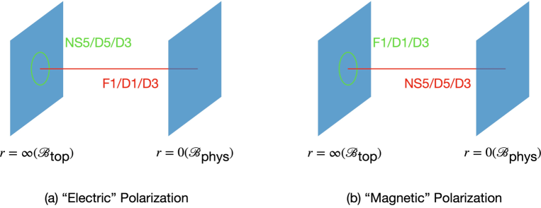
Figure 3: Brane origins of symmetry operators and charged objects under different polarizations, namely different topological boundary conditions. $r$ is the coordinate of the radial direction for the conical singularity of the Calabi-Yau 4-fold $Y$. At $r=0$, we have the singularity probed by D1-branes, while at $r=\infty$, boundary conditions for various SymTFT fields are picked. Symmetry operators are engineered from branes at $r=\infty$ (colored in green), while charged defects are built from branes terminating at $r=\infty$ (colored in red).

Note that the above discussion also reproduces (82), namely the invertible symmetry $G^{a^{(k)}}$ and its non-invertible symmetry promotion correspond to the same operator in the SymTFT bulk, whose stringy origin is a D3-brane.

The anomalies of these non-invertible symmetries are encoded back in the linking invariant (92). If elements in the set $\{L_{(k)}^{\text{D3}}\}\subset\{L_{(i)}^{\text{D3}}\}$ generating the $G^{a^{(k)}}$ and the non-invertible defects $\mathcal{N}_{(k)}$ always have non-trivial linking among them, then it is not possible to simultaneously condensing all lines in $\{L_{(k)}^{\text{D3}}\}$. This implies an anomaly via the obstruction to the gapped boundary condition as an obstruction to gauging the $G^{a^{(k)}}$ symmetry or gauging the non-invertible symmetry generated by $\mathcal{N}_{(k)}$.

4.2.2 Hanany-Witten Transition

One of the typical properties of non-invertible symmetry operators is their behavior when passing through the charged objects. In 2D, moving a non-invertible line operator past a genuine local operator leaves behind another topological line attached to a defect operator and a T-shape junction. See Figure 4 (a).

This non-trivial action of non-invertible symmetries admits a string theory interpretation as the Hanany-Witten transition [103]. Consider the “magnetic” polarization (77) where the associated 2D QFTs enjoy TY$(\Gamma_{2}^{(j)}\times\Gamma_{2}^{(j)})$ categorical symmetry. One can build local charge operators from

$$\text{$(p,q)$ 5-brane wrapping on cone}(\gamma_{5(j)})$$ (97)

where $p$ and $q$ label the D5-brane and NS5-brane charges, respectively. Recall that these wrapping branes are sources for the $\widehat{b}$ and $\widehat{c}$ fields in the SymTFT (68), implying their linkings with D1-strings and F1-strings, as discussed in (65). Therefore, the above $(p,q)$ 5-brane gives rise to the local operator carrying charge $(q,p)$ under the invertible part $G^{(\widehat{b}_{(j)})}\times G^{(\widehat{c}_{(j)})}$ within the TY$(\Gamma_{2}^{(j)}\times\Gamma_{2}^{(j)})$ categorical symmetry:

$$\text{$(p,q)$ 5-brane wrapping on cone}(\gamma_{5(j)})$$

$$\updownarrow$$

$$\text{$(q,p)$-charged local operator under $G^{(\widehat{b}_{(j)})}\times G^{(\widehat{c}_{(j)})}$}.$$

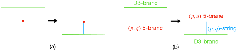
Figure 4: (a) Motion of the non-invertible symmetry operator passing through a local operator. A topological line is created, attaching to the non-invertible line and the local operator. (b) This non-trivial action is realized in string theory as the Hanany-Witten transition. The string theory origins for various field-theoretic objects are given by (90), (91), and (97).

Now, consider a wrapped D3-brane moving through this $(p,q)$ 5-brane along the transverse direction of the 2D spacetime. A $(p,q)$-string will be created and attached between the D3-brane and the $(p,q)$ 5-brane. This created string is exactly the topological line operator (91) generating the $G^{(\widehat{b}_{(j)})}\times G^{(\widehat{c}_{(j)})}$ symmetry. This Hanany-Witten transition configuration exactly matches the non-trivial action of the non-invertible symmetry line on local charged objects. See Figure 4 (b). We remark that this Hananay-Witten origin for actions of non-invertible symmetries is ubiquitous for QFTs admitting string theory embeddings. See, e.g., [40, 43, 52, 44].

5 Examples

In this section, we discuss explicit examples of 2D QFTs engineered from Calabi-Yau 4-folds with D1-brane probes. The following three subsections correspond to the three facets of our general discussion in previous sections: intrinsic relativeness, non-invertible symmetries, and the manifestation of their anomalies as obstructions to gauging.

5.1 $Y^{p,k}(\mathbb{P}^{2})$: When are they Intrinsically Relative?

In Section 4.1.1, we obtained a sufficient condition for the intrinsic relativeness of 2D QFTs associated with Calabi-Yau 4-folds. We now apply this condition to an infinite class of Calabi-Yau 4-folds, namely cones over Sasaki-Einstein 7-manifold $Y=Y^{p,k}(\mathbb{P}^{2})$.

The toric data of this class of Calabi-Yau 4-folds is given by a convex polytope with ${\mathbb{Z}}^{4}$ coordinates [82]

$$p_{1}=(0,0,0,1),p_{2}=(0,0,p,1),p_{3}=(1,0,0,1),p_{4}=(0,1,0,1),p_{5}=(-1,-1,k,1).$$ (98)

The associated 2D QFTs living on D1-brane probes have quiver gauge theory descriptions constructed in [104], to which we refer the reader for more details.

The Sasaki-Einstein base space $Y^{p,k}(\mathbb{P}^{2})$ gives rise to the asymptotic boundary $\partial Y$, with the cohomology classes [82]

$$H^{*}(S^{7}/{\mathbb{Z}}_{2};{\mathbb{Z}})=\left\{\mathbb{Z},0,{\mathbb{Z}}\oplus{\mathbb{Z}}_{\text{gcd}(p,k)},0,\Gamma_{4},{\mathbb{Z}},{\mathbb{Z}}_{\text{gcd}(p,k)},\mathbb{Z}\right\},$$ (99)

where $\Gamma_{4}={\mathbb{Z}}^{2}/\langle(0,-3p+k),(k,p)\rangle$. Using the Smith normal form decomposition, we can derive the general result (see also [51])

$$\Gamma_{4}={\mathbb{Z}}_{\text{gcd}(p,k)}\times{\mathbb{Z}}_{\frac{k(3p-k)}{\text{gcd}(p,k)}}.$$ (100)

It is easy to see the second, fourth, and sixth cohomology classes are purely torsional: $\text{Tor}H^{(i)}(S^{7}/{\mathbb{Z}}_{2};{\mathbb{Z}}_{2})=H^{(i)}(S^{7}/{\mathbb{Z}}_{2};{\mathbb{Z}}_{2}),i=2,4,6$. For each of these classes, there is one corresponding differential cohomology generator

$$\breve{t}_{i}\in\breve{H}^{i}(S^{7}/{\mathbb{Z}}_{2}).$$ (101)

The expansion of differential cohomology uplifts of various IIB fluxes in this example is

$$\begin{split}\breve{F}_{6}=&\breve{a}_{4}\star\breve{t}_{2}+\breve{a}_{2}^{(1)}\star\breve{t}_{4(1)}+\breve{a}_{2}^{(2)}\star\breve{t}_{4(2)}\cdots,\\ \breve{H}_{3}=&\breve{b}_{1}\star\breve{t}_{2}+\cdots,\\ \breve{G}_{3}=&\breve{c}_{1}\star\breve{t}_{2}+\cdots,\end{split}$$ (102)

where we label the background fields for ${\mathbb{Z}}_{\text{gcd}(p,k)}$ and ${\mathbb{Z}}_{\frac{k(3p-k)}{\text{gcd}(p,k)}}$ by cochains $\breve{a}_{1}^{(1)}$ and $\breve{a}_{1}^{(2)}$, respectively. The corresponding SymTFT terms in (68) read

$$2\pi\int_{M_{3}}\Lambda_{i_{1}i_{2}}a_{1}^{(i_{1})}\cup\delta a_{1}^{(i_{2})}.$$ (103)

As we discussed in Section 2 and Section 4.1.1, a sufficient condition for intrinsic relativeness is when $|\Gamma_{4}|$ is not a perfect square, due to the absence of the Lagrangian subgroup of the defect group. For this class of theories, we arrive at the following statement:

$$\boxed{\text{\emph{The 2D QFT for $Y^{p,k}(\mathbb{P}^{2})$ is intrinsically relative if $k(3p-k)$ is not a perfect square.}}}$$

One can perform a similar analysis for other classes of theories, e.g., orbifold singularities and $Y^{p,k}(\mathbb{P}^{1}\times\mathbb{P}^{1})$, and obtain the sufficient condition for 2D QFTs being intrinsically relative. In the following subsections, we will focus on Calabi-Yau 4-folds admitting absolute QFTs and their non-invertible symmetries, possibly with anomalies.

5.2 $Y^{2,0}(\mathbb{P}^{1}\times\mathbb{P}^{1})$: Rep$(D_{4})$ Symmetry

Let us now consider the Calabi-Yau 4-fold given by the cone over the Sasaki-Einstein 7-manifold $Y^{2,0}(\mathbb{P}^{1}\times\mathbb{P}^{1})$, which belongs to an infinite class of geometries known as $Y^{p,k}(B_{4})$ [82], where $B_{4}$ denotes a four-dimensional base space that is either $\mathbb{P}^{1}\times\mathbb{P}^{1}$ or $\mathbb{P}^{2}$. The 2D QFTs associated with this general class of Calabi-Yau 4-folds were systematically constructed and studied in [104]. The toric data for $Y^{2,0}(\mathbb{P}^{1}\times\mathbb{P}^{1})$ is given by the polytope with the following vertex coordinates in ${\mathbb{Z}}^{4}$ [104]

$$\begin{split}&p_{1}=(1,1,0,0),p_{2}=(1,0,1,0),p_{3}=(1,-1,0,0),p_{4}=(1,0,-1,0),p_{5}=(1,0,0,2),\\ &s=(1,0,0,1),q=(1,0,0,0)\end{split}$$ (104)

The associated 2D QFT living on D1-brane probes enjoys a quiver gauge theory description, with quiver diagram given in Figure 5. We refer the reader to [75, 104] additional details on this theory.

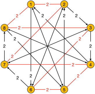
Figure 5: Quiver diagram for $Y^{2,0}(\mathbb{P}^{1}\times\mathbb{P}^{1})$ probed by D1-branes

The SymTFT for finite symmetries of this 2D QFT was constructed in [52]. Here, we revisit the result and present some further discussion. The cohomology classes of $Y^{2,0}(\mathbb{P}^{1}\times\mathbb{P}^{1})$ read

$$H^{*}(Y^{2,0}(\mathbb{P}^{1}\times\mathbb{P}^{1});{\mathbb{Z}})=\left\{\mathbb{Z},0,\mathbb{Z}^{2}\oplus\mathbb{Z}_{2},0,\mathbb{Z}\oplus\mathbb{Z}_{2}\oplus\mathbb{Z}_{2},\mathbb{Z}^{2},\mathbb{Z}_{2},\mathbb{Z}\right\}$$ (105)

The differential cohomology generators for torsional parts read

$$\begin{split}&\breve{t}_{2}\in\breve{H}^{2}(Y^{2,0}(\mathbb{P}^{1}\times\mathbb{P}^{1})),~{}\breve{t}_{6}\in\breve{H}^{6}(Y^{2,0}(\mathbb{P}^{1}\times\mathbb{P}^{1}))\\ &\breve{t}_{4(1)}\in\breve{H}^{4}(Y^{2,0}(\mathbb{P}^{1}\times\mathbb{P}^{1})),~{}\breve{t}_{4(2)}\in\breve{H}^{4}(Y^{2,0}(\mathbb{P}^{1}\times\mathbb{P}^{1})),\end{split}$$ (106)

The expansion of uplifts of various IIB fluxes is

$$\begin{split}\breve{F}_{6}=&\breve{a}_{4}\star\breve{t}_{2}+\breve{a}_{2}\star\breve{t}_{4(1)}+\breve{\widehat{a}}_{2}\star\breve{t}_{4(2)}\cdots,\\ \breve{H}_{3}=&\breve{b}_{1}\star\breve{t}_{2}+\cdots,\\ \breve{G}_{3}=&\breve{c}_{1}\star\breve{t}_{2}+\cdots.\end{split}$$ (107)

The linking numbers between various cohomology generators are given by [52]

$$\begin{split}&\Lambda_{21}=\Lambda_{12}=\int\breve{t}_{4(1)}\star\breve{t}_{4(2)}~{}\text{mod 1}=\frac{1}{2},\\ ~{}&\Delta_{i}=-\int\breve{t}_{4(1)}\star\breve{t}_{2}\star\breve{t}_{2}~{}\text{mod 1}=\frac{1}{2},\\ &\Omega=\int\breve{t}_{2}\star\breve{t}_{6}=\frac{1}{2}.\end{split}$$ (108)

Substituting these linking numbers in the general form of the SymTFT (68), one obtains the SymTFT for the $Y^{2,0}(\mathbb{P}^{1}\times\mathbb{P}^{1})$ theory [52]

$$S_{3}=\frac{2\pi}{2}\int_{M_{3}}a_{1}\cup\delta\widehat{a}_{1}+b_{1}\cup\delta\widehat{b}_{1}+c_{1}\cup\delta\widehat{c}_{1}+a_{1}\cup b_{1}\cup c_{1}$$ (109)

where all fields are ${\mathbb{Z}}_{2}$ cochains, whose differential cochain counterparts are in (107) under obvious notations.

The topological line operators in this SymTFT can be computed from brane actions explicitly, following the steps in Section 4.2. Substituting the linking numbers (108) into the general results for wrapped D3-brane (90), F1-string and D1-string (91), one obtains

$$\begin{split}&L^{D3}_{(1)}=\exp\left(\pi i\int_{M_{1}}\widehat{a}_{1}\right)\times\int{\mathcal{D}}\widehat{\phi}_{0}{\mathcal{D}}\phi_{0}\exp\left(\pi i\int_{M_{1}}\widehat{\phi}_{0}\cup\delta\phi_{0}+c_{1}\cup\phi_{0}-b_{1}\cup\widehat{\phi}_{0}\right),\\ &L^{D3}_{(2)}=\exp\left(\pi i\int_{M_{1}}a_{1}\right),~{}L^{\text{F1}}=\exp\left(\pi i\int_{M_{1}}b_{1}\right),~{}L^{\text{D1}}=\exp\left(\pi i\int_{M_{1}}c_{1}\right).\end{split}$$ (110)

In addition to the four line operators above, it is also possible to derive other two operators from NS5-brane and D5-brane wrapping on the torsional 5-cycle $\gamma_{5}$, following the same steps in Section 4.2,

$$\begin{split}L^{\text{NS5}}=\exp\left(\pi i\int_{M_{1}}\widehat{b}_{1}\right)\times\int{\mathcal{D}}\widehat{\phi}_{0}{\mathcal{D}}\phi_{0}\exp\left(\pi i\int_{M_{1}}\widehat{\phi}_{0}\cup\delta\phi_{0}+c_{1}\cup\phi_{0}-a_{1}\cup\widehat{\phi}_{0}\right),\\ L^{\text{D5}}=\exp\left(\pi i\int_{M_{1}}\widehat{c}_{1}\right)\times\int{\mathcal{D}}\widehat{\phi}_{0}{\mathcal{D}}\phi_{0}\exp\left(\pi i\int_{M_{1}}\widehat{\phi}_{0}\cup\delta\phi_{0}+a_{1}\cup\phi_{0}-b_{1}\cup\widehat{\phi}_{0}\right),\end{split}$$ (111)

“Electric” boundary condition for anomalous $({\mathbb{Z}}_{2})^{3}$ symmetry.

The generic “electric” boundary condition (74) in this example is

$$a_{1},b_{1},c_{1}~{}\text{Dirichlet},~{}\widehat{a}_{1},\widehat{b}_{1},\widehat{c}_{1}~{}\text{Neumann}.$$ (112)

Under this boundary condition, on the one hand, the three invertible line operators in the second line of (110) are trivialized along the gapped boundary. This, in turn, leads to the fact the D3-brane on $\gamma_{3}^{(2)}$, F1-string and D1-string on $\gamma_{1}$ can end “at infinity”, serving as the heavy charged objects. See Figure 6 (a) for a schematic depiction. On the other hand, the three non-invertible lines $L^{\text{D3}}_{(1)},L^{\text{NS5}}$ and $L^{\text{D5}}$ are reduced to their invertible parts, generating the three ${\mathbb{Z}}_{2}$ symmetries

$$G^{(0)}=\mathbb{Z}_{2}^{(a)}\times\mathbb{Z}_{2}^{(b)}\times\mathbb{Z}_{2}^{(c)},$$ (113)

aligning with the general form in (75) for the resulting absolute QFT. This $({\mathbb{Z}}_{2})^{3}$ symmetry has an anomaly given by the following 3D invertible TFT

$$\exp\left(\pi i\int_{M_{3}}A\cup B\cup C\right),$$ (114)

where $A,B$, and $C$ are background profiles for the $a_{1},b_{1}$ and $c_{1}$ under Dirichlet gapped boundary conditions.

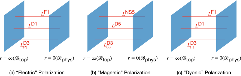
Figure 6: Brane origins for local operators in 2D QFTs for $Y^{(2,0)}(\mathbb{P}^{1}\times\mathbb{P}^{1})$ under various boundary conditions at infinity. The global symmetries for these three polarizations are discussed in the main text as (a) Anomalous $({\mathbb{Z}}_{2})^{3}$ symmetry, (b) Rep$(D_{4})$ symmetry, and (c) $D_{4}$ symmetry.

“Magnetic” boundary condition for Rep($D_{4}$) symmetry.

The generic “magnetic” boundary condition (77) via gauging the ${\mathbb{Z}}_{2}^{(b)}\times{\mathbb{Z}}_{2}^{(c)}$ symmetry is

$$a_{1},\widehat{b}_{1},\widehat{c}_{1}~{}\text{Dirichlet},~{}\widehat{a}_{1},b_{1},c_{1}~{}\text{Neumann}.$$ (115)

Under this boundary condition, on the one hand, line operators $L_{(2)}^{\text{D3}},L^{\text{NS5}}$ and $L^{\text{D5}}$ trivialize along the gapped boundary, on which they terminate and serve as charged defects for the 2D QFT. See Figure 6 (b) for an illustration. Interestingly, the non-invertible part of $L^{\text{D3}}_{(1)}$ survives in this case. Together with the invertible topological lines $L^{\text{F1}}$ and $L^{\text{D1}}$, this generates a non-invertible symmetry with TY$({\mathbb{Z}}_{2}\times{\mathbb{Z}}_{2})$ fusion rules

$$\begin{split}&L^{\text{D3}}_{(1)}\otimes L^{\text{D3}}_{(1)}=1\oplus L^{\text{F1}}\oplus L^{\text{D1}}\oplus L^{\text{F1}}L^{\text{D1}},\\ &L^{\text{D3}}_{(1)}\otimes L^{\text{F1}}=L^{\text{F1}}\otimes L^{\text{D3}}_{(1)}=L^{\text{D3}}_{(1)},\\ &L^{\text{D3}}_{(1)}\otimes L^{\text{D1}}=L^{\text{D1}}\otimes L^{\text{D3}}_{(1)}=L^{\text{D3}}_{(1)},\\ &L^{\text{F1}}\otimes L^{\text{F1}}=L^{\text{D1}}\otimes L^{\text{F1}}=1.\end{split}$$ (116)

The fusion rules, in general, do not fully fix the fusion category. For the TY$({\mathbb{Z}}_{2}\times{\mathbb{Z}}_{2})$ non-invertible symmetry, there are four fusion categories that obey the same fusion rules, three of which are non-anomalous, namely Rep$(D_{4})$, Rep$(Q_{8})$ and Rep$(\mathcal{H}_{8})$ (see, e.g., [5, 9, 68, 69]). In order to identify the non-invertible symmetry with the above fusion rules, we can consider gauging the full non-invertible symmetry, which corresponds to the “dyonic” gapped boundary condition below for the SymTFT.

“Dyonic” boundary condition for $D_{4}$ symmetry.

Starting with the “electric” boundary condition with $({\mathbb{Z}}_{2})^{3}$ symmetry, we can consider gauging the ${\mathbb{Z}}_{2}^{(a)}$ symmetry, and end up with the following “dyonic” boundary condition

$$\widehat{a}_{1},b_{1},c_{1}~{}\text{Dirichlet},~{}a_{1},\widehat{b}_{1},\widehat{c}_{1}~{}\text{Neumann}.$$ (117)

Under this condition, there are three ${\mathbb{Z}}_{2}$ symmetries ${\mathbb{Z}}_{2}^{(\widehat{a})}$, ${\mathbb{Z}}_{2}^{(b)}$ and ${\mathbb{Z}}_{2}^{(c)}$ with respective background field profiles $\widehat{A},B$ and $C$ under Dirichlet boundary conditions. See Figure 6 (c) for brane origins of charged defects under this polarization. However, the genuine global symmetry here is not a direct product of the three ${\mathbb{Z}}_{2}$ factors, due to the extra condition

$$\delta\widehat{A}=BC$$ (118)

inherited from the equation of motion of $a$ in the SymTFT. According to [105] (see also [107, 5, 108, 109]), the above equation leads to a group extension ${\mathbb{Z}}_{2}^{(\widehat{a})}\rtimes({\mathbb{Z}}_{2}^{(b)}\times{\mathbb{Z}}_{2}^{(c)})=D_{4}$.

The “magnetic” boundary condition (115) can then be derived from gauging the whole $D_{4}$ symmetry. Note that the non-invertible topological line $L^{\text{D3}}_{(1)}$ generating the Rep$(D_{4})$ symmetry under “magenetic” condition now ends at infinity and becomes charged defects under “dyonic” condition. See Figure 6 (c) for an illustration. This identifies the non-invertible symmetry with TY$({\mathbb{Z}}_{2}\times{\mathbb{Z}}_{2})$ fusion rules (116) as the Rep$(D_{4})$ categorical symmetry [5] and aligns with the fact that the Rep$(D_{4})$ symmetry is non-anomalous and gaugeable with $D_{4}$ quantum symmetry.

5.3 $\mathbb{C}^{4}/\mathbb{Z}_{4}$: Anomalies of the Non-invertible Symmetry

The local Calabi-Yau 4-fold ${\mathbb{C}}^{4}/{\mathbb{Z}}_{4}$ is defined by the following orbifold action

$$(z_{1},z_{2},z_{3},z_{4})\rightarrow(e^{\pi i/2}z_{1},e^{\pi i/2}z_{2},e^{\pi i/2}z_{3},e^{\pi i/2}z_{4}).$$ (119)

The toric data of ${\mathbb{C}}^{4}/{\mathbb{Z}}_{4}$ is given by the polytope whose vertices have the following ${\mathbb{Z}}^{4}$ coordinates

$$p_{1}=(1,1,0,0),p_{2}=(1,0,1,0),p_{3}=(1,0,0,1),p_{4}=(1,-1,-1,-1),q=(1,0,0,0).$$ (120)

The associated 2D QFT living on D1-brane probes has a quiver gauge theory description. Figure 7 shows the corresponding quiver diagram.

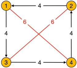
Figure 7: Quiver diagram for ${\mathbb{C}}^{4}/{\mathbb{Z}}_{4}$ probed by D1-branes.

We refer the reader to [71] for detailed information on this theory.

The asymptotic boundary in this case is simply the seven-dimensional lens space $S^{7}/{\mathbb{Z}}_{4}$, whose cohomology classes read

$$H^{*}(S^{7}/{\mathbb{Z}}_{2};{\mathbb{Z}})=\left\{\mathbb{Z},0,{\mathbb{Z}}_{4},0,{\mathbb{Z}}_{4},0,{\mathbb{Z}}_{4},\mathbb{Z}\right\}.$$ (121)

The expansion of differential uplifts of various IIB fluxes is the same as in ${\mathbb{C}}^{4}/{\mathbb{Z}}_{4}$

$$\begin{split}\breve{F}_{6}=&\breve{a}_{4}\star\breve{t}_{2}+\breve{a}_{2}\star\breve{t}_{4}+\cdots,\\ \breve{H}_{3}=&\breve{b}_{1}\star\breve{t}_{2}+\cdots,\\ \breve{G}_{3}=&\breve{c}_{1}\star\breve{t}_{2}+\cdots,\end{split}$$ (122)

The linking numbers between various cohomology generators can be computed as (see also [51])

$$\begin{split}&\Lambda_{21}=\Lambda_{12}=\int\breve{t}_{4}\star\breve{t}_{4}~{}\text{mod 1}=\frac{1}{4},\\ ~{}&\Delta_{i}=-\int\breve{t}_{4}\star\breve{t}_{2}\star\breve{t}_{2}~{}\text{mod 1}=\frac{1}{4},\\ &\Omega=\int\breve{t}_{2}\star\breve{t}_{6}=\frac{1}{4}.\end{split}$$ (123)

Substituting these linking numbers in the general form of the SymTFT (68), one obtains the SymTFT for the ${\mathbb{C}}^{4}/{\mathbb{Z}}_{4}$ theory

$$S_{3}=\frac{2\pi}{4}\int_{M_{3}}\frac{1}{2}a_{1}\cup\delta a_{1}+b_{1}\cup\delta\widehat{b}_{1}+c_{1}\cup\delta\widehat{c}_{1}-a_{1}\cup b_{1}\cup c_{1},$$ (124)

where all gauge fields are ${\mathbb{Z}}_{4}$-valued cochains, whose differential cochain counterparts are in (122) under obvious notations. The defect group is given by

$$\mathbb{D}={\mathbb{Z}}_{4}^{(a)}\times{\mathbb{Z}}_{4}^{(b)}\times{\mathbb{Z}}_{4}^{(\widehat{b})}\times{\mathbb{Z}}_{4}^{(c)}\times{\mathbb{Z}}_{4}^{(\widehat{c})},$$ (125)

with Dirac pairing matrix extracted from the coefficients of the single-derivative terms in the SymTFT

$$\begin{pmatrix}{\color[rgb]{1,0,0}\frac{1}{4}}&0&0&0&0\\ 0&0&\frac{1}{4}&0&0\\ 0&\frac{1}{4}&0&0&0\\ 0&0&0&0&\frac{1}{4}\\ 0&0&0&\frac{1}{4}&0\\ \end{pmatrix}.$$ (126)

The topological line operators from D3-branes, F1-strings and D1-strings can be computed from the general form in (90) and (91) using the linking number (123):

$$\begin{split}&L^{D3}=\exp\left(\frac{\pi i}{2}\int_{M_{1}}\widehat{a}_{1}\right)\times\int{\mathcal{D}}\widehat{\phi}_{0}{\mathcal{D}}\phi_{0}\exp\left(\frac{\pi i}{2}\int_{M_{1}}\widehat{\phi}_{0}\cup\delta\phi_{0}+c_{1}\cup\phi_{0}-b_{1}\cup\widehat{\phi}_{0}\right),\\ &L^{\text{F1}}=\exp\left(\frac{\pi i}{2}\int_{M_{1}}b_{1}\right),~{}L^{\text{D1}}=\exp\left(\frac{\pi i}{2}\int_{M_{1}}c_{1}\right).\end{split}$$ (127)

One can compute similarly line operators from NS5-branes and D5-branes wrapping on the torsional 5-cycle. Their concrete expression is not important for our following discussion, so we will just simply donote them as $L^{\text{NS5}}$ and $L^{\text{D5}}$.

“Electric” boundary condition for ${\mathbb{Z}}_{2}\times({\mathbb{Z}}_{4})^{2}$ symmetry.

First, consider the polarization with the following Lagrangian subgroup

$$L={\mathbb{Z}}_{2}^{(a)}\times{\mathbb{Z}}_{4}^{(\widehat{b})}\times{\mathbb{Z}}_{4}^{(\widehat{c})}.$$ (128)

The corresponding gapped boundary condition of the SymTFT for $b_{1}$ and $c_{1}$ are standard Dirichlet boundary conditions, while for $a_{1}$ it is a bit special:

$$a_{1}|_{\partial M_{3}}=A_{1}.$$ (129)

Similarly to (32), the above condition constrains the ${\mathbb{Z}}_{4}$-valued $a_{1}$ to a ${\mathbb{Z}}_{2}$-valued background gauge field profile $A_{1}$, implying the quotient by ${\mathbb{Z}}_{2}^{(a)}\subset{\mathbb{Z}}_{4}^{(a)}$ Lagrangian subgroup. In the SymTFT language, this is to say $L^{\text{D3}}$ does not compose any Lagrangian subalgebra, namely there is no gapped boundary for it to ends. However, condensing the subalgebra $1\oplus(L^{\text{D3}})^{2}$ is admitted, and it define a topological boundary on which $(L^{\text{D3}})^{2}$ can end. From the string theory perspective, this means the boundary condition at infinity does not allow a single D3-brane to end, but a collection of two D3-branes can terminate at infinity, giving rise to the charged defect. See Figure 8 (a) for an illustration.

The resulting absolute QFT enjoys an invertible $({\mathbb{Z}}_{2})^{3}$ global symmetry, as discussed in the general form (75), reading

$$G=L^{\vee}={\mathbb{Z}}_{2}^{\vee}\times{\mathbb{Z}}_{4}^{(b)}\times{\mathbb{Z}}_{4}^{(c)},$$ (130)

with ${\mathbb{Z}}_{2}^{\vee}={\mathbb{Z}}_{4}^{(a)}/{\mathbb{Z}}_{2}^{(a)}$ due to the exact sequence

$$1\rightarrow{\mathbb{Z}}_{2}^{(a)}\rightarrow{\mathbb{Z}}_{4}^{(a)}\rightarrow{\mathbb{Z}}_{2}^{\vee}\rightarrow 1.$$ (131)

Furthermore, this ${\mathbb{Z}}_{2}\times({\mathbb{Z}}_{4})^{2}$ symmetry suffers from anomalies captured by the following invertible 3D TFT

$$\frac{2\pi}{4}\int_{M_{3}}A_{1}\cup\delta A_{1}-A_{1}\cup B_{1}\cup C_{1}.$$ (132)

where $B_{1}$ and $C_{1}$ are Dirichlet boundary profiles for $b_{1}$ and $c_{1}$ fields. In the above invertible TFT, the first term shows a self ’t Hooft anomaly for the ${\mathbb{Z}}_{2}^{\vee}$ symmetry, while the second cubic term captures a mixed anomaly between ${\mathbb{Z}}_{2}^{\vee}$, ${\mathbb{Z}}_{4}^{(b)}$ and ${\mathbb{Z}}_{4}^{(c)}$.

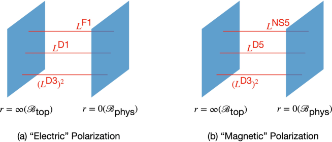
Figure 8: Brane origins for local operators in 2D QFTs for ${\mathbb{C}}^{4}/{\mathbb{Z}}_{4}$ under various boundary conditions at infinity. $(L^{(D3)})^{2}$ is engineered from a collection of two D3-branes. The global symmetries for these three polarizations are discussed in the main text as (a) Anomalous ${\mathbb{Z}}_{2}\times({\mathbb{Z}}_{4})^{2}$ symmetry, and (b) Anomalous TY(${\mathbb{Z}}_{4}\times{\mathbb{Z}}_{4}$) non-invertible symmetry.

“Magnetic” boundary condition for anomalous TY$({\mathbb{Z}}_{4}\times Z_{4})$ symmetry.

Based on our discussion in Section 4, one can gauge the ${\mathbb{Z}}_{4}^{(b)}\times{\mathbb{Z}}_{4}^{(c)}$ symmetry and end up with the following Lagrangian subgroup

$$L={\mathbb{Z}}_{2}^{(a)}\times{\mathbb{Z}}_{4}^{(b)}\times{\mathbb{Z}}_{4}^{(c)}.$$ (133)

The corresponding gapped boundary condition of the SymTFT for $a_{1}$ is not changed, but now $\widehat{b}_{1}$ and $\widehat{c}_{1}$ get Dirichlet boundary conditions. In order to read the global symmetry for the resulting absolute QFT, notice that the associated quotient for the defect group is

$$L^{\vee}=\mathbb{D}/L\cong{\mathbb{Z}}_{2}^{\vee}\times{\mathbb{Z}}_{4}^{(\widehat{b})}\times{\mathbb{Z}}_{4}^{(\widehat{c})}.$$ (134)

However, this is not the genuine global symmetry. Instead, with the presence of the cubic anomaly term $(2\pi/4)\int_{M_{3}}A_{1}\cup B_{1}\cup C_{1}$ in (132) under the “electric” polarization, the ${\mathbb{Z}}_{2}^{\vee}$ part is not a direct product with the other two factors but is promoted to a non-trivial ${\mathbb{Z}}_{2}$ extension. The resulting symmetry reads

$$\text{TY$({\mathbb{Z}}_{4}^{(\widehat{b})}\times{\mathbb{Z}}_{4}^{(\widehat{c})})$ fusion categorical symmetry}.$$ (135)

The fusion rules, falling in the general form (79), for this non-invertible symmetry can be computed explicitly from the topological line operators engineered from D3-brane, F1-string and D1-string in (127).

According to our discussion in Sections 2.3.2 and 4.2.1, it is now straightforward to see that this non-invertible symmetry is anomalous. Let us assume this symmetry is gaugeable. From the defect group point of view, this is to say there is a polarization for which the Lagrangian subgroup is given by the $L^{\vee}$ uplift. However, due to the $\frac{1}{4}$ factor in red in (126), $L^{\vee}$ cannot be embedded back in the $\mathbb{D}$ as a Lagrangian subgroup. This means the assumed polarization of the defect group obtained from gauging the TY$({\mathbb{Z}}_{4}\times{\mathbb{Z}}_{4})$ symmetry, in fact, does not exist, implying this non-invertible symmetry is anomalous. From the SymTFT and its string theory origin point of view, this translates to the fact that only a collection of two D3-branes wrapping on torsional 3-cycles are allowed to end at infinity, due to the self-linking property of D3-branes. This prevents the existence of a “dyonic” boundary condition (named after the $Y^{(2,0)}(\mathbb{P}^{1}\times\mathbb{P}^{1})$ example in Section 5.2), where other lines built from D3-branes can terminate. In other words, the boundary condition after an attempt of gauging TY$({\mathbb{Z}}_{4}\times{\mathbb{Z}}_{4})$ symmetry is obstructed, implying an anomaly of this non-invertible symmetry.

We thank I. Garcia Etxebarria, J. J. Heckman, M. Hübner, H. T. Lam, Y.-H. Lin, S. Schafer-Nameki, S.-H. Shao, E. Sharpe, E. Torres, Y. Wang, H. Y. Zhang, and Y. Zheng for helpful discussions. XY thanks J. J. Heckman, M. Hübner, C. Lawrie, E. Torres, and H. Y. Zhang for their collaboration on related projects. We thank the 2023 Simons Summer Workshop for hospitality during part of this work. XY thanks the 2023 NYU Satellite Workshop on Global Categorical Symmetries, the 2023 Annual Meeting of the Simons Collaboration on Global Categorical Symmetries, and the 2024 Spring Southeastern Regional Mathematical String Theory Meeting for hospitality during part of this work. SF is supported by the U.S. National Science Foundation grants PHY-2112729 and DMS-1854179. XY is supported by NSF grant PHY-2014086.

References

- [1] D. Gaiotto, A. Kapustin, N. Seiberg, and B. Willett, “Generalized Global Symmetries,” JHEP 02 (2015) 172, arXiv:1412.5148 [hep-th].
- [2] E. P. Verlinde, “Fusion Rules and Modular Transformations in 2D Conformal Field Theory,” Nucl. Phys. B 300 (1988) 360–376.
- [3] J. Fuchs, I. Runkel, and C. Schweigert, “TFT construction of RCFT correlators 1. Partition functions,” Nucl. Phys. B 646 (2002) 353–497, arXiv:hep-th/0204148.
- [4] J. Frohlich, J. Fuchs, I. Runkel, and C. Schweigert, “Kramers-Wannier duality from conformal defects,” Phys. Rev. Lett. 93 (2004) 070601, arXiv:cond-mat/0404051.
- [5] L. Bhardwaj and Y. Tachikawa, “On finite symmetries and their gauging in two dimensions,” JHEP 03 (2018) 189, arXiv:1704.02330 [hep-th].
- [6] C.-M. Chang, Y.-H. Lin, S.-H. Shao, Y. Wang, and X. Yin, “Topological Defect Lines and Renormalization Group Flows in Two Dimensions,” JHEP 01 (2019) 026, arXiv:1802.04445 [hep-th].
- [7] R. Thorngren and Y. Wang, “Fusion Category Symmetry I: Anomaly In-Flow and Gapped Phases,” arXiv:1912.02817 [hep-th].
- [8] Z. Komargodski, K. Ohmori, K. Roumpedakis, and S. Seifnashri, “Symmetries and strings of adjoint QCD2,” JHEP 03 (2021) 103, arXiv:2008.07567 [hep-th].
- [9] R. Thorngren and Y. Wang, “Fusion Category Symmetry II: Categoriosities at = 1 and Beyond,” arXiv:2106.12577 [hep-th].
- [10] P. Etingof, D. Nikshych, and V. Ostrik, “On fusion categories,” arXiv:math/0203060.
- [11] N. Reshetikhin and V. G. Turaev, “Invariants of three manifolds via link polynomials and quantum groups,” Invent. Math. 103 (1991) 547–597.
- [12] V. G. Turaev and O. Y. Viro, “State sum invariants of 3 manifolds and quantum 6j symbols,” Topology 31 (1992) 865–902.
- [13] J. W. Barrett and B. W. Westbury, “Invariants of piecewise linear three manifolds,” Trans. Am. Math. Soc. 348 (1996) 3997–4022, arXiv:hep-th/9311155.
- [14] E. Witten, “AdS / CFT correspondence and topological field theory,” JHEP 12 (1998) 012, arXiv:hep-th/9812012.
- [15] A. Kirillov, Jr. and B. Balsam, “Turaev-Viro invariants as an extended TQFT,” arXiv:1004.1533 [math.GT].
- [16] A. Kapustin and N. Saulina, “Surface operators in 3d Topological Field Theory and 2d Rational Conformal Field Theory,” arXiv:1012.0911 [hep-th].
- [17] A. Kitaev and L. Kong, “Models for Gapped Boundaries and Domain Walls,” Commun. Math. Phys. 313 no. 2, (2012) 351–373, arXiv:1104.5047 [cond-mat.str-el].
- [18] J. Fuchs, C. Schweigert, and A. Valentino, “Bicategories for boundary conditions and for surface defects in 3-d TFT,” Commun. Math. Phys. 321 (2013) 543–575, arXiv:1203.4568 [hep-th].
- [19] D. S. Freed and C. Teleman, “Relative quantum field theory,” Commun. Math. Phys. 326 (2014) 459–476, arXiv:1212.1692 [hep-th].
- [20] D. S. Freed and C. Teleman, “Topological dualities in the Ising model,” Geom. Topol. 26 (2022) 1907–1984, arXiv:1806.00008 [math.AT].
- [21] D. S. Freed, G. W. Moore, and C. Teleman, “Topological symmetry in quantum field theory,” arXiv:2209.07471 [hep-th].
- [22] J. Kaidi, K. Ohmori, and Y. Zheng, “Symmetry TFTs for Non-Invertible Defects,” arXiv:2209.11062 [hep-th].
- [23] A. Antinucci, F. Benini, C. Copetti, G. Galati, and G. Rizi, “The holography of non-invertible self-duality symmetries,” arXiv:2210.09146 [hep-th].
- [24] L. Bhardwaj and S. Schafer-Nameki, “Generalized Charges, Part I: Invertible Symmetries and Higher Representations,” arXiv:2304.02660 [hep-th].
- [25] L. Bhardwaj and S. Schafer-Nameki, “Generalized Charges, Part II: Non-Invertible Symmetries and the Symmetry TFT,” arXiv:2305.17159 [hep-th].
- [26] F. Baume, J. J. Heckman, M. Hübner, E. Torres, A. P. Turner, and X. Yu, “SymTrees and Multi-Sector QFTs,” arXiv:2310.12980 [hep-th].
- [27] L. Bhardwaj, L. E. Bottini, D. Pajer, and S. Schafer-Nameki, “The Club Sandwich: Gapless Phases and Phase Transitions with Non-Invertible Symmetries,” arXiv:2312.17322 [hep-th].
- [28] T. D. Brennan and Z. Sun, “A SymTFT for Continuous Symmetries,” arXiv:2401.06128 [hep-th].
- [29] A. Antinucci and F. Benini, “Anomalies and gauging of U(1) symmetries,” arXiv:2401.10165 [hep-th].
- [30] R. Argurio, F. Benini, M. Bertolini, G. Galati, and P. Niro, “On the Symmetry TFT of Yang-Mills-Chern-Simons theory,” arXiv:2404.06601 [hep-th].
- [31] F. Bonetti, M. Del Zotto, and R. Minasian, “SymTFTs for Continuous non-Abelian Symmetries,” arXiv:2402.12347 [hep-th].
- [32] F. Apruzzi, F. Bedogna, and N. Dondi, “SymTh for non-finite symmetries,” arXiv:2402.14813 [hep-th].
- [33] L. Bhardwaj, D. Pajer, S. Schafer-Nameki, and A. Warman, “Hasse Diagrams for Gapless SPT and SSB Phases with Non-Invertible Symmetries,” arXiv:2403.00905 [cond-mat.str-el].
- [34] M. Del Zotto, S. N. Meynet, and R. Moscrop, “Remarks on Geometric Engineering, Symmetry TFTs and Anomalies,” arXiv:2402.18646 [hep-th].
- [35] I. n. Garcia Etxebarria and S. S. Hosseini, “Some aspects of symmetry descent,” arXiv:2404.16028 [hep-th].
- [36] C. Zhang and C. Córdova, “Anomalies of categorical symmetries,” arXiv:2304.01262 [cond-mat.str-el].
- [37] J. Kaidi, E. Nardoni, G. Zafrir, and Y. Zheng, “Symmetry TFTs and Anomalies of Non-Invertible Symmetries,” arXiv:2301.07112 [hep-th].
- [38] C. Cordova, P.-S. Hsin, and C. Zhang, “Anomalies of Non-Invertible Symmetries in (3+1)d,” arXiv:2308.11706 [hep-th].
- [39] A. Antinucci, F. Benini, C. Copetti, G. Galati, and G. Rizi, “Anomalies of non-invertible self-duality symmetries: fractionalization and gauging,” arXiv:2308.11707 [hep-th].
- [40] F. Apruzzi, I. Bah, F. Bonetti, and S. Schafer-Nameki, “Noninvertible Symmetries from Holography and Branes,” Phys. Rev. Lett. 130 no. 12, (2023) 121601, arXiv:2208.07373 [hep-th].
- [41] I. Garcia Etxebarria, “Branes and Non-Invertible Symmetries,” Fortsch. Phys. 70 no. 11, (2022) 2200154, arXiv:2208.07508 [hep-th].
- [42] J. J. Heckman, M. Hübner, E. Torres, and H. Y. Zhang, “The Branes Behind Generalized Symmetry Operators,” arXiv:2209.03343 [hep-th].
- [43] J. J. Heckman, M. Hubner, E. Torres, X. Yu, and H. Y. Zhang, “Top down approach to topological duality defects,” Phys. Rev. D 108 no. 4, (2023) 046015, arXiv:2212.09743 [hep-th].
- [44] F. Apruzzi, F. Bonetti, D. S. W. Gould, and S. Schafer-Nameki, “Aspects of Categorical Symmetries from Branes: SymTFTs and Generalized Charges,” arXiv:2306.16405 [hep-th].
- [45] I. Bah, E. Leung, and T. Waddleton, “Non-Invertible Symmetries, Brane Dynamics, and Tachyon Condensation,” arXiv:2306.15783 [hep-th].
- [46] M. Dierigl, J. J. Heckman, M. Montero, and E. Torres, “R7-Branes as Charge Conjugation Operators,” arXiv:2305.05689 [hep-th].
- [47] M. Cvetivc, J. J. Heckman, M. Hübner, and E. Torres, “Fluxbranes, Generalized Symmetries, and Verlinde’s Metastable Monopole,” arXiv:2305.09665 [hep-th].
- [48] B. S. Acharya, M. Del Zotto, J. J. Heckman, M. Hubner, and E. Torres, “Junctions, Edge Modes, and -Holonomy Orbifolds,” arXiv:2304.03300 [hep-th].
- [49] C. Lawrie, X. Yu, and H. Y. Zhang, “Intermediate defect groups, polarization pairs, and noninvertible duality defects,” Phys. Rev. D 109 no. 2, (2024) 026005, arXiv:2306.11783 [hep-th].
- [50] F. Apruzzi, F. Bonetti, I. Garcia Etxebarria, S. S. Hosseini, and S. Schafer-Nameki, “Symmetry TFTs from String Theory,” arXiv:2112.02092 [hep-th].
- [51] M. van Beest, D. S. W. Gould, S. Schafer-Nameki, and Y.-N. Wang, “Symmetry TFTs for 3d QFTs from M-theory,” arXiv:2210.03703 [hep-th].
- [52] X. Yu, “Non-invertible Symmetries in 2D from Type IIB String Theory,” arXiv:2310.15339 [hep-th].
- [53] I. Basile and G. Leone, “Anomaly constraints for heterotic strings and supergravity in six dimensions,” JHEP 04 (2024) 067, arXiv:2310.20480 [hep-th].
- [54] N. Braeger, V. Chakrabhavi, J. J. Heckman, and M. Hubner, “Generalized Symmetries of Non-Supersymmetric Orbifolds,” arXiv:2404.17639 [hep-th].
- [55] S. Deser, A. Gomberoff, M. Henneaux, and C. Teitelboim, “P-brane dyons and electric magnetic duality,” Nucl. Phys. B 520 (1998) 179–204, arXiv:hep-th/9712189.
- [56] G. ’t Hooft, “On the phase transition towards permanent quark confinement,” Nuclear Physics B 138 no. 1, (1978) 1–25. https://www.sciencedirect.com/science/article/pii/0550321378901530.
- [57] D. Belov and G. W. Moore, “Holographic Action for the Self-Dual Field,” arXiv:hep-th/0605038.
- [58] S. Gukov, P.-S. Hsin, and D. Pei, “Generalized global symmetries of theories. Part I,” JHEP 04 (2021) 232, arXiv:2010.15890 [hep-th].
- [59] A. Kapustin and N. Saulina, “Topological boundary conditions in abelian Chern-Simons theory,” Nucl. Phys. B 845 (2011) 393–435, arXiv:1008.0654 [hep-th].
- [60] J. Kaidi, G. Zafrir, and Y. Zheng, “Non-invertible symmetries of = 4 SYM and twisted compactification,” JHEP 08 (2022) 053, arXiv:2205.01104 [hep-th].
- [61] Y. Tachikawa, “On the 6d origin of discrete additional data of 4d gauge theories,” JHEP 05 (2014) 020, arXiv:1309.0697 [hep-th].
- [62] D. Mumford, M. Nori, and P. Norman, Tata Lectures on Theta III. Modern Birkhäuser Classics. Birkhäuser Boston, 2006. https://books.google.com/books?id=Y6mn6ILOAN8C.
- [63] Y. Choi, B. C. Rayhaun, Y. Sanghavi, and S.-H. Shao, “Remarks on boundaries, anomalies, and noninvertible symmetries,” Phys. Rev. D 108 no. 12, (2023) 125005, arXiv:2305.09713 [hep-th].
- [64] C. G. Callan, Jr. and J. A. Harvey, “Anomalies and Fermion Zero Modes on Strings and Domain Walls,” Nucl. Phys. B 250 (1985) 427–436.
- [65] R. Dijkgraaf and E. Witten, “Topological Gauge Theories and Group Cohomology,” Commun. Math. Phys. 129 (1990) 393.
- [66] M. Levin and Z.-C. Gu, “Braiding statistics approach to symmetry-protected topological phases,” Phys. Rev. B 86 (2012) 115109, arXiv:1202.3120 [cond-mat.str-el].
- [67] D. Tambara and S. Yamagami, “Tensor categories with fusion rules of self-duality for finite abelian groups,” Journal of Algebra 209 no. 2, (1998) 692–707. https://www.sciencedirect.com/science/article/pii/S0021869398975585.
- [68] A. Perez-Lona, D. Robbins, E. Sharpe, T. Vandermeulen, and X. Yu, “Notes on gauging noninvertible symmetries. Part I. Multiplicity-free cases,” JHEP 02 (2024) 154, arXiv:2311.16230 [hep-th].
- [69] O. Diatlyk, C. Luo, Y. Wang, and Q. Weller, “Gauging Non-Invertible Symmetries: Topological Interfaces and Generalized Orbifold Groupoid in 2d QFT,” arXiv:2311.17044 [hep-th].
- [70] Y. Choi, C. Cordova, P.-S. Hsin, H. T. Lam, and S.-H. Shao, “Noninvertible duality defects in 3+1 dimensions,” Phys. Rev. D 105 no. 12, (2022) 125016, arXiv:2111.01139 [hep-th].
- [71] S. Franco, D. Ghim, S. Lee, R.-K. Seong, and D. Yokoyama, “2d (0,2) Quiver Gauge Theories and D-Branes,” JHEP 09 (2015) 072, arXiv:1506.03818 [hep-th].
- [72] S. Franco, S. Lee, and R.-K. Seong, “Brane Brick Models, Toric Calabi-Yau 4-Folds and 2d (0,2) Quivers,” JHEP 02 (2016) 047, arXiv:1510.01744 [hep-th].
- [73] S. Franco, S. Lee, and R.-K. Seong, “Brane brick models and 2d (0, 2) triality,” JHEP 05 (2016) 020, arXiv:1602.01834 [hep-th].
- [74] S. Franco, S. Lee, R.-K. Seong, and C. Vafa, “Brane Brick Models in the Mirror,” JHEP 02 (2017) 106, arXiv:1609.01723 [hep-th].
- [75] S. Franco, S. Lee, and R.-K. Seong, “Orbifold Reduction and 2d (0,2) Gauge Theories,” JHEP 03 (2017) 016, arXiv:1609.07144 [hep-th].
- [76] S. Franco and A. Hasan, “ printing of gauge theories,” JHEP 05 (2018) 082, arXiv:1801.00799 [hep-th].
- [77] S. Franco, D. Ghim, S. Lee, and R.-K. Seong, “Elliptic Genera of 2d (0,2) Gauge Theories from Brane Brick Models,” JHEP 06 (2017) 068, arXiv:1702.02948 [hep-th].
- [78] S. Franco and X. Yu, “BFT2: a general class of 2d = (0, 2) theories, 3-manifolds and toric geometry,” JHEP 08 (2022) 277, arXiv:2107.00667 [hep-th].
- [79] S. Franco, D. Ghim, G. P. Goulas, and R.-K. Seong, “Mass deformations of brane brick models,” JHEP 09 (2023) 176, arXiv:2307.03220 [hep-th].
- [80] D. S. Freed, G. W. Moore, and G. Segal, “The Uncertainty of Fluxes,” Commun. Math. Phys. 271 (2007) 247–274, arXiv:hep-th/0605198.
- [81] D. S. Freed, G. W. Moore, and G. Segal, “Heisenberg Groups and Noncommutative Fluxes,” Annals Phys. 322 (2007) 236–285, arXiv:hep-th/0605200.
- [82] D. Martelli and J. Sparks, “Notes on toric Sasaki-Einstein seven-manifolds and AdS(4) / CFT(3),” JHEP 11 (2008) 016, arXiv:0808.0904 [hep-th].
- [83] A. Hatcher, Algebraic Topology. Cambridge University Press, 2002.
- [84] S. Franco, A. Mininno, A. M. Uranga, and X. Yu, “2d = (0, 1) gauge theories and Spin(7) orientifolds,” JHEP 03 (2022) 150, arXiv:2110.03696 [hep-th].
- [85] S. Franco, A. Mininno, A. M. Uranga, and X. Yu, “Spin(7) orientifolds and 2d = (0, 1) triality,” JHEP 01 (2022) 058, arXiv:2112.03929 [hep-th].
- [86] I. Bah, F. Bonetti, and R. Minasian, “Discrete and higher-form symmetries in SCFTs from wrapped M5-branes,” JHEP 03 (2021) 196, arXiv:2007.15003 [hep-th].
- [87] C.-T. Hsieh, Y. Tachikawa, and K. Yonekura, “Anomaly Inflow and p-Form Gauge Theories,” Commun. Math. Phys. 391 no. 2, (2022) 495–608, arXiv:2003.11550 [hep-th].
- [88] D. M. Belov and G. W. Moore, “Type II Actions from 11-Dimensional Chern-Simons Theories,” arXiv:hep-th/0611020.
- [89] S. Monnier, “Canonical quadratic refinements of cohomological pairings from functorial lifts of the Wu class,” arXiv:1208.1540 [math.AT].
- [90] J. J. Heckman and L. Tizzano, “6D Fractional Quantum Hall Effect,” JHEP 05 (2018) 120, arXiv:1708.02250 [hep-th].
- [91] J.-L. Brylinski, Loop spaces, characteristic classes and geometric quantization. Springer Science & Business Media, 2007.
- [92] J. Cheeger and J. Simons, “Differential characters and geometric invariants,” 1985. https://api.semanticscholar.org/CorpusID:50800553.
- [93] C. Baer and C. Becker, “Differential characters and geometric chains,” 2013.
- [94] K. Hori, S. Katz, A. Klemm, R. Pandharipande, R. Thomas, C. Vafa, R. Vakil, and E. Zaslow, Mirror symmetry, vol. 1 of Clay mathematics monographs. AMS, Providence, USA, 2003.
- [95] P. G. Camara, L. E. Ibanez, and F. Marchesano, “RR photons,” JHEP 09 (2011) 110, arXiv:1106.0060 [hep-th].
- [96] M. Del Zotto, J. J. Heckman, D. S. Park, and T. Rudelius, “On the Defect Group of a 6D SCFT,” Lett. Math. Phys. 106 no. 6, (2016) 765–786, arXiv:1503.04806 [hep-th].
- [97] I. Garcia Etxebarria, B. Heidenreich, and D. Regalado, “IIB flux non-commutativity and the global structure of field theories,” JHEP 10 (2019) 169, arXiv:1908.08027 [hep-th].
- [98] J. Kaidi, K. Ohmori, and Y. Zheng, “Kramers-Wannier-like Duality Defects in (3+1)D Gauge Theories,” Phys. Rev. Lett. 128 no. 11, (2022) 111601, arXiv:2111.01141 [hep-th].
- [99] K. Roumpedakis, S. Seifnashri, and S.-H. Shao, “Higher Gauging and Non-invertible Condensation Defects,” arXiv:2204.02407 [hep-th].
- [100] M. Etheredge, I. Garcia Etxebarria, B. Heidenreich, and S. Rauch, “Branes and symmetries for S-folds,” arXiv:2302.14068 [hep-th].
- [101] M. R. Douglas, “Branes within branes,” NATO Sci. Ser. C 520 (1999) 267–275, arXiv:hep-th/9512077.
- [102] R. G. Leigh, “Dirac-Born-Infeld Action from Dirichlet Sigma Model,” Mod. Phys. Lett. A 4 (1989) 2767.
- [103] A. Hanany and E. Witten, “Type IIB superstrings, BPS monopoles, and three-dimensional gauge dynamics,” Nucl. Phys. B 492 (1997) 152–190, arXiv:hep-th/9611230.
- [104] S. Franco, D. Ghim, and R.-K. Seong, “Brane brick models for the Sasaki-Einstein 7-manifolds Yp,k(1× 1) and Yp,k(2),” JHEP 03 (2023) 050, arXiv:2212.02523 [hep-th].
- [105] M. D. F. de Wild Propitius, Topological interactions in broken gauge theories. PhD thesis, Amsterdam U., 1995. arXiv:hep-th/9511195.
- [106] G. Kac, “Finite group rings,” Trans. Moscow Math. Soc. 15 (1966) 251–294.
- [107] Y. Tachikawa, “On gauging finite subgroups,” SciPost Phys. 8 no. 1, (2020) 015, arXiv:1712.09542 [hep-th].
- [108] J. Wang and X.-G. Wen, “Non-Abelian string and particle braiding in topological order: Modular SL(3,) representation and (3+1) -dimensional twisted gauge theory,” Phys. Rev. B 91 no. 3, (2015) 035134, arXiv:1404.7854 [cond-mat.str-el].
- [109] L. Bhardwaj, L. E. Bottini, L. Fraser-Taliente, L. Gladden, D. S. W. Gould, A. Platschorre, and H. Tillim, “Lectures on Generalized Symmetries,” arXiv:2307.07547 [hep-th].