Edge Importance in Complex Networks

Abstract

Complex networks are made up of vertices and edges. The latter connect the vertices. There are several ways to measure the importance of the vertices, e.g., by counting the number of edges that start or end at each vertex, or by using the subgraph centrality of the vertices. It is more difficult to assess the importance of the edges. One approach is to consider the line graph associated with the given network and determine the importance of the vertices of the line graph, but this is fairly complicated except for small networks. This paper compares two approaches to estimate the importance of edges of medium-sized to large networks. One approach computes partial derivatives of the total communicability of the weights of the edges, where a partial derivative of large magnitude indicates that the corresponding edge may be important. Our second approach computes the Perron sensitivity of the edges. A high sensitivity signals that the edge may be important. The performance of these methods and some computational aspects are discussed. Applications of interest include to determine whether a network can be replaced by a network with fewer edges with about the same communicability.

Keywords: Network analysis, Sensitivity analysis, Edge importance

1 Introduction

Networks are helpful for modeling complex interactions between entities. A network can be represented by a graph $\mathcal{G}=\langle\mathcal{V},\mathcal{E},\mathcal{W}\rangle$, which consists of a set of vertices or nodes $\mathcal{V}=\{v_{1},v_{2},\dots,v_{n}\}$, a set of edges $\mathcal{E}=\{e_{1},e_{2},\dots,e_{m}\}$ that connect the vertices, and a set of nonnegative edge weights $\mathcal{W}=\{w_{11},w_{21},\ldots,w_{nn}\}$. The weight $w_{ij}$ is positive if there is an edge pointing from vertex $v_{i}$ to vertex $v_{j}$; while $w_{ij}=0$ signifies that there is no such edge. Edges may be directed (and then model one-way streets) or undirected (and then model two-way streets). If the graph models a road network in which the vertices model intersections and the edges model roads, then the weights may, e.g., be proportional to the amount of traffic along each road. A network in which all positive weights are one is said to be unweighted. Descriptions and many applications of networks are provided by, e.g., Estrada [11] and Newman [19].

We say that vertex $v_{i}$ is directly connected to vertex $v_{j}$ if there is a single edge from vertex $v_{i}$ pointing to vertex $v_{j}$. Vertex $v_{j}$ is then said to be adjacent to vertex $v_{i}$. When the edge between these vertices is undirected, vertex $v_{j}$ also is directly connected to vertex $v_{i}$, and $v_{i}$ is adjacent to vertex $v_{j}$. Vertex $v_{i}$ is said to be indirectly connected to vertex $v_{j}$ if the latter vertex can be reached from the former by following at least two edges from $v_{i}$. We will consider graphs without multiple edges and without edges that start and end at the same vertex.

Let $e(v_{i}\rightarrow v_{j})$ denote an edge from vertex $v_{i}$ to $v_{j}$. If there also is an edge $e(v_{j}\rightarrow v_{i})$ and $w_{ij}=w_{ji}>0$, then the edge is said to be undirected and denoted by $e(v_{i}\leftrightarrow v_{j})$. A sequence of edges (not necessarily distinct)

$$\{e(v_{1}\to v_{2}),e(v_{2}\to v_{3}),\dots,e(v_{k}\to v_{k+1})\}$$

forms a walk. The length of a walk is the sum of the weights of the edges that make up the walk, i.e., $\sum_{i=1}^{k}w_{i,i+1}$. If the edges in a walk are distinct, then the walk is referred to as a path.

Introduce the adjacency matrix $\mathbf{A}=[w_{ij}]_{i,j=1}^{n}\in\mathbb{R}^{n\times n}$ associated with the graph $\mathcal{G}$. The adjacency matrix $\mathbf{A}$ is sparse in most applications, i.e., the matrix has many more zero entries than positive entries. The matrix is symmetric if for each edge there also is an edge in the opposite direction with the same weight. The graph determined by such an adjacency matrix is said to be undirected. If at least one edge of a graph is directed, or if $w_{ij}\neq w_{ji}$ for at least one index pair $\{i,j\}$, then the graph is said to be directed. The adjacency matrix associated with a directed graph is nonsymmetric. Since we assume that there are no edges that start and end at the same vertex, the diagonal entries of the adjacency matrix $\mathbf{A}$ vanish.

Let $\exp_{0}(t)=\exp(t)-1$ and consider the power series expansion

$$\exp_{0}(\mathbf{A})=\mathbf{A}+\frac{\mathbf{A}^{2}}{2!}+\frac{\mathbf{A}^{3}}{3!}+\ldots~{}.$$ (1)

Let $\mathbf{A}^{k}=[a_{ij}^{(k)}]_{i,j=1}^{n}$ for $k=1,2,\ldots~{}$, where $a_{ij}^{(1)}=w_{ij}$ for $1\leq i,j\leq n$. A nonvanishing entry $a_{ij}^{(k)}$ for some $k>0$ indicates that there is at least one walk of $k$ edges from vertex $v_{i}$ to vertex $v_{j}$. The denominators in the terms of the expansion (1) ensure that the expansion converges and that terms $\frac{\mathbf{A}^{k}}{k!}$ with $k$ large contribute only little to $\exp(\mathbf{A})$. It follows that short walks typically are more important than long ones, which is in agreement with the intuition that messages propagate better along short walks than along long ones. This led Estrada and Rodriguez-Velazquez [13] to use $\exp(\mathbf{A})$ to study properties of a graph; we use the function $\exp_{0}(\mathbf{A})$ because the term with the identity matrix $\mathbf{I}$ in the expansion of $\exp(\mathbf{A})$ has no natural interpretation in the context of network modeling. Other functions also can be used such as a resolvent or a Mittag-Leffler function; see Estrada and Higham [12] and Arrigo and Durastante [2] for discussions.

Estrada and Rodriguez-Velazquez [13] define for graphs with a symmetric adjacency matrix the communicability matrix $\exp(\mathbf{A})$; we will use the matrix

$$\mathbf{C}=[c_{ij}]_{i,j=1}^{n}=\exp_{0}(\mathbf{A}).$$

The entry $c_{ij}$, $i\neq j$, is referred to as the communicability between the vertices $v_{i}$ and $v_{j}$. A relatively large value implies that it is easy for the vertices $v_{i}$ and $v_{j}$ to communicate. Estrada and Rodriguez-Velazquez [13] measure the importance of the vertex $v_{i}$ of an undirected graph by the subgraph centrality $c_{ii}+1$; we will use $c_{ii}$. Related measures of communicability can be defined when the adjacency matrix $\mathbf{A}$ is nonsymmetric; see [6].

We define the total communicability of the graph $\mathcal{G}$ as

$$T_{\mathcal{G}}(w_{11},w_{21},\ldots,w_{nn})=e^{T}\exp_{0}(\mathbf{A})e,$$ (2)

where $e=[1,1,\ldots,1]^{T}\in\mathbb{R}^{n}$ denotes the vector with all entries $1$ and the superscript ^T stands for transposition. Benzi and Klymko [3] introduced the related measure $e^{T}\exp(\mathbf{A})e$, which differs from (2) by the additive constant $n$. Note that the expression (2) is invariant under transposition. We have

$$T_{\mathcal{G}}(w_{11},w_{21},\ldots,w_{nn})=e^{T}\exp_{0}(\mathbf{A}^{T})e=\frac{1}{2}e^{T}(\exp_{0}(\mathbf{A})+\exp_{0}(\mathbf{A}^{T}))e.$$

The graph associated with the adjacency matrix $\mathbf{A}^{T}$ is known as the reverse graph to ${\mathcal{G}}$. Thus, the total communicability of the graph ${\mathcal{G}}$ and of the reverse graph are the same.

We are interested in investigating the importance of the edges of a graph ${\mathcal{G}}$ and, in particular, in determining which edge weights can be reduced or set to zero without significantly affecting the total communicability. A possible approach to investigate the importance of edges is to consider the line graph associated with the graph. The edges of ${\mathcal{G}}$ correspond to vertices in the associated line graph, and the importance of the edges in ${\mathcal{G}}$ can be measured by the subgraph centrality of the vertices of the line graph. This approach is investigated in [7, 8]. However, it is quite cumbersome to construct the line graph except for small graphs. A simple heuristic technique was proposed by Arrigo and Benzi [1], who define the importance of an edge in terms of the importance of the vertices where the edge starts and ends. However, this approach is not guaranteed to correctly rank the importance of edges; see [7, Section 5.4] for an example. More recently an approach that uses the right and left Perron vectors of the adjacency matrix in combination with the Wilkinson perturbation to determine which weights to increase in order to increase the total communicability has been described in [4, 21]. An analogous technique is applied in [10] to discern which weights in a weighted multilayer network can be decreased without affecting the total communicability significantly.

Another approach to study the importance of edges is to evaluate the Fréchet derivatives of the total communicability (2) with respect to the weights. This approach was advocated by De la Cruz Cabrera et al. [4] and recently Schweitzer [27] described how to speed up the computations. Introduce the gradient

$$\nabla T_{\mathcal{G}}(w_{11},w_{21},\ldots,w_{nn})=\left[\frac{\partial}{\partial w_{11}}e^{T}\exp_{0}(\mathbf{A})e,\frac{\partial}{\partial w_{21}}e^{T}\exp_{0}(\mathbf{A})e,\ldots,\frac{\partial}{\partial w_{nn}}e^{T}\exp_{0}(\mathbf{A})e\right]^{T}.$$ (3)

When the partial derivative

$$\frac{\partial}{\partial w_{ij}}e^{T}\exp_{0}(\mathbf{A})e$$ (4)

is (relatively) large, a small increase in the positive weight $w_{ij}$ results in a substantial change in the total communicability. We will show below that the partial derivatives (4) are nonnegative.

For example, let the graph represent a road map, where the edges model roads and the vertices represent intersections of roads. Let vertex $v_{j}$ be adjacent to vertex $v_{i}$. Then widening an existing road from $v_{i}$ to $v_{j}$ may result in a significant increase in the total communicability of the graph; the widening of this road is modeled by increasing the weight $w_{ij}$. Also, when (4) is relatively large, and vertex $v_{j}$ is not adjacent to vertex $v_{i}$, i.e., there is no road from $v_{i}$ to $v_{j}$, building such a road may increase the total communicability substantially. This is modeled by making the vanishing weight $w_{ij}$ positive.

Conversely, if the partial derivative (4) is relatively small and the weight $w_{ij}>0$ is small, then setting $w_{ij}$ to zero, i.e., removing the edge from vertex $v_{i}$ to vertex $v_{j}$, will not affect the total communicability (2) much. This implies that blocking the road from vertex $v_{i}$ to $v_{j}$, e.g., due to construction, does not change the total communicability of the network significantly.

This paper is organized as follows. Section 2 discusses how the gradient can be applied to assess the importance of edges. The first part of the section is concerned with small to medium-sized problems for which it is feasible to evaluate the gradient (3). The latter part of the section discusses the application of Krylov subspace methods to project large-scale problems to problems of fairly small size. The computations use a result by Schweitzer [27] on the evaluation of Fréchet derivatives, but differ in various aspects. Section 3 reviews methods described in [4, 10, 21] based on evaluating the right and left Perron vectors and the Wilkinson perturbation to determine important and unimportant edges. Numerical examples are reported in Section 4. These examples compare the methods of Sections 2 and 3. Section 5 contains concluding remarks.

We conclude this section with comments on some related methods. A scheme that combines regression, soft-thresholding, and projection is applied in [5] to approximate an unweighted network by a simpler unweighted network. This scheme performs well but may be expensive and is restricted to unweighted networks. Massei and Tudisco [17] consider the problem of determining a low-rank perturbation $\mathbf{E}\in\mathbb{R}^{n\times n}$ to the adjacency matrix $\mathbf{A}$ so that the perturbed matrix $\mathbf{A}+\mathbf{E}$ maximizes the robustness of the network. For instance, $\mathbf{E}$ may be chosen to maximize the trace of $f(\mathbf{A}+\mathbf{E})-f(\mathbf{A})$ for a user-specified matrix-valued function $f$. The perturbation $\mathbf{E}$ is determined by a greedy algorithm for solving an optimization problem. A careful comparison with this method is outside the scope of the present paper.

2 Network modifications based on the gradient

This section discusses methods for modifying, adding, or removing edges of a network by using information furnished by the gradient (3). We first describe methods for small to medium-sized networks for which all entries of the gradient (3) can be evaluated. Subsequently, we will consider Krylov subspace methods that can be applied to large-scale networks.

2.1 Methods for small to medium-sized networks

Let the matrix function $f:\mathbf{A}\in\mathbb{R}^{n\times n}\to f(\mathbf{A})\in\mathbb{R}^{n\times n}$ be continuously differentiable sufficiently many times in a region in the complex plane that contains all eigenvalues of $\mathbf{A}$. Then the function $f$ has a Fréchet derivative $L_{f}(\mathbf{A},\mathbf{E})\in\mathbb{R}^{n\times n}$ at $\mathbf{A}$ in the direction $\mathbf{E}\in\mathbb{R}^{n\times n}$ for all matrices $\mathbf{E}$ of sufficiently small norm. The Fréchet derivative satisfies

$$f(\mathbf{A}+\mathbf{E})=f(\mathbf{A})+L_{f}(\mathbf{A},\mathbf{E})+o(\|\mathbf{E}\|),$$ (5)

as $\|\mathbf{E}\|\to 0$, where $\|\cdot\|$ is any matrix norm; see, e.g., [15] for details. Schweitzer described an efficient approach to evaluate $L_{f}(\mathbf{A},\mathbf{E})$ in several directions $\mathbf{E}$ simultaneously.

THEOREM 1.

(Schweitzer [27, Theorem 2.3]) Let $\mathbf{A}\in\mathbb{R}^{n\times n}$ and $u,v\in\mathbb{R}^{n}\backslash\{0\}$, and assume that $f$ is Fréchet differentiable at $\mathbf{A}$. Define $\mathbf{E}_{ij}=e_{i}e_{j}^{T}$, where $e_{k}=[0,\ldots,0,1,0,\ldots,0]^{T}\in\mathbb{R}^{n}$ denotes the $k$th column of the identity matrix. Then

$$u^{T}L_{f}(\mathbf{A},\mathbf{E}_{ij})v=e_{i}^{T}L_{f}(\mathbf{A}^{T},uv^{T})e_{j}.$$ (6)

Thus, the entries of the matrix $L_{f}(\mathbf{A}^{T},uv^{T})$ furnish Fréchet derivatives in all directions $\mathbf{E}_{ij}=e_{i}e_{j}^{T}$, $1\leq i,j\leq n$. We are primarily interested in the situation when $f(t)=\exp_{0}(t)$ and

$$u=v=e=[1,1,\ldots,1]^{T}\in\mathbb{R}^{n}.$$ (7)

THEOREM 2.

All entries of the gradient (3) are nonnegative.

Proof.

Let $\mathbf{E}_{ij}=e_{i}e_{j}^{T}$. Then for $f(t)=\exp_{0}(t)$, we have

$$\frac{\partial}{\partial w_{ij}}e^{T}\exp_{0}(\mathbf{A})e=e^{T}L_{f}(\mathbf{A},\mathbf{E}_{ij})e.$$

It follows from (5) that

$$L_{f}(\mathbf{A},h\mathbf{E}_{ij})=\exp_{0}(\mathbf{A}+h\mathbf{E}_{ij})-\exp_{0}(\mathbf{A})+o(h)~{}~{}\mbox{as}~{}~{}h\searrow 0.$$

The power series expansion of $f(t)=\exp_{0}(t)$ gives

$$L_{f}(\mathbf{A},h\mathbf{E}_{ij}) = h\left(\mathbf{E}_{ij}+\frac{\mathbf{A}\mathbf{E}_{ij}+\mathbf{A}\mathbf{E}_{ij}}{2!}+\frac{\mathbf{A}^{2}\mathbf{E}_{ij}+\mathbf{A}\mathbf{E}_{ij}\mathbf{A}+\mathbf{E}_{ij}\mathbf{A}^{2}}{3!}+\ldots~{}\right)+o(h)$$

$$= h\left(\sum_{\ell=1}^{\infty}\sum_{k=0}^{\ell-1}\mathbf{A}^{k}\mathbf{E}_{ij}\mathbf{A}^{\ell-1-k}+o(1)\right).$$

Each term in the above sum is a matrix with nonnegative entries. Hence, the sum is a matrix with nonnegative entries. The term $o(1)$ vanishes as $h\searrow 0$. Since $L_{f}(\mathbf{A},h\mathbf{E}_{ij})$ is linear in $h$, we obtain

$$L_{f}(\mathbf{A},\mathbf{E}_{ij})=\lim_{h\searrow 0}\frac{L_{f}(\mathbf{A},h\mathbf{E}_{ij})}{h}=\sum_{\ell=1}^{\infty}\sum_{k=0}^{\ell-1}\mathbf{A}^{k}\mathbf{E}_{ij}\mathbf{A}^{\ell-1-k}.$$ (8)

This completes the proof. ∎

A possible way to evaluate the matrix $L_{f}(\mathbf{A}^{T},uv^{T})$ in (6) when $\mathbf{A}^{T}\in\mathbb{R}^{n\times n}$ is to use the relation

$$f\left(\left[\begin{array}[]{cc}\mathbf{A}^{T}&uv^{T}\\ \mathbf{0}&\mathbf{A}^{T}\end{array}\right]\right)=\left[\begin{array}[]{cc}f(\mathbf{A}^{T})&L_{f}(\mathbf{A}^{T},uv^{T})\\ \mathbf{0}&f(\mathbf{A}^{T})\end{array}\right];$$ (9)

see, e.g., [15, p. 253]. However, when $f(t)=\exp_{0}(t)$, the computation of $f(\mathbf{A}^{T})$ requires ${\mathcal{O}}(n^{3})$ arithmetic floating point operations (flops). Therefore, the evaluation of the left-hand side of (9) demands about $8$ times more flops than the calculation of $f(\mathbf{A}^{T})$. It is cheaper to approximate $L_{f}(\mathbf{A}^{T},uv^{T})$ by using the finite-difference approximation

$$L_{f}(\mathbf{A}^{T},uv^{T})\approx\frac{f(\mathbf{A}^{T}+huv^{T})-f(\mathbf{A}^{T}-huv^{T})}{2h}$$ (10)

for some $h>0$. We will use $h=\frac{2}{n}\cdot 10^{-4}$ in the computed examples in Section 4. This is suggested by the following simple computations. We have used the fact that $\|uv^{T}\|_{2}=n$, which holds for the vectors (7). Here and throughout this paper $\|\cdot\|_{2}$ denotes the spectral matrix norm or the Euclidean vector norm.

Example 2.1. Let $f(t)=\exp_{0}(t)$ be evaluated with a relative error $\delta_{t}$ bounded by $\delta>0$ and let $h>0$ be a small scalar. Then

$$\frac{f(t+h)-f(t-h)}{2h} \approx \frac{f_{\text{exact}}(t+h)+\delta_{t+h}f_{\text{exact}}(t)-(f_{\text{exact}}(t-h)+\delta_{t-h}f_{\text{exact}}(t))}{2h}$$

$$\approx f_{\text{exact}}^{\prime}(t)+\frac{h^{2}}{6}f_{\text{exact}}^{\prime\prime\prime}(t)+\frac{\delta_{t+h}-\delta_{t-h}}{2h}f_{\text{exact}}(t).$$

Thus, the error is bounded by about

$$\left(\frac{h^{2}}{6}+\frac{\delta}{h}\right)\exp(t).$$

Minimization over $h>0$ yields

$$h\approx(3\delta)^{1/3}.$$

The computation of the scalar exponential is carried out with high relative accuracy in MATLAB. However, evaluation of the matrix exponential $\exp(\mathbf{A}^{T})$ is more difficult. It can be computed in several ways; see, e.g., [15, Chapter 10] as well as [24, 30]. The accuracy achieved depends on the method use as well as on the size and properties of the matrix $\mathbf{A}^{T}$; see, e.g., [15, Chapter 10] and [24] for computed examples. We therefore include a factor $10^{3}$ in the bound $\delta$ for the relative accuracy. This bound is valid for most matrices of sizes of interest to us. Letting $\delta\approx 10^{3}\epsilon_{\text{mach}}$ with $\epsilon_{\text{mach}}\approx 2\cdot 10^{-16}$ gives $h\approx 2\cdot 10^{-4}$.   $\Box$

THEOREM 3.

Let $f(t)=\exp_{0}(t)$. Then

$$\frac{f(\mathbf{A}^{T}+h\mathbf{E}_{ij})-f(\mathbf{A}^{T}-h\mathbf{E}_{ij})}{2h}=L_{f}(\mathbf{A}^{T},\mathbf{E}_{ij})+O(h^{2}).$$

Proof.

The right-hand side of (10) with $uv^{T}$ replaced with $\mathbf{E}_{ij}$ can be expressed as

$$\frac{f(\mathbf{A}^{T}+h\mathbf{E}_{ij})-f(\mathbf{A}^{T}-h\mathbf{E}_{ij})}{2h} = \mathbf{E}_{ij}+\frac{1}{2!}(\mathbf{A}^{T}\mathbf{E}_{ij}+\mathbf{E}_{ij}\mathbf{A}^{T})$$

$$+ \frac{1}{3!}((\mathbf{A}^{T})^{2}\mathbf{E}_{ij}+\mathbf{A}^{T}\mathbf{E}_{ij}\mathbf{A}^{T}+\mathbf{E}_{ij}(\mathbf{A}^{T})^{2})$$

$$+ \frac{1}{4!}((\mathbf{A}^{T})^{3}\mathbf{E}_{ij}+(\mathbf{A}^{T})^{2}\mathbf{E}_{ij}\mathbf{A}^{T}+\mathbf{A}^{T}\mathbf{E}_{ij}(\mathbf{A}^{T})^{2}+\mathbf{E}_{ij}(\mathbf{A}^{T})^{3})$$

$$+ \ldots~{}+O(h^{2}).$$

The result now follows from (8) with $\mathbf{A}$ replaced by $\mathbf{A}^{T}$. ∎

The evaluation of the right-hand side of (10) with $f(t)=\exp_{0}(t)$ gives approximations of all the entries of the gradient (3). We will refer to $\|\nabla T_{\mathcal{G}}(w_{11},w_{21},\ldots,w_{nn})\|_{2}$ as the total transmission of the graph ${\mathcal{G}}$.

2.1.1 Network simplification by edge removal

One of the aims of this paper is to discuss how to reduce the complexity of a network by removing edges without changing the total transmission or total communicability significantly. A simple way to achieve the former is to set positive weights $w_{ij}$ to zero when the associated entries of the gradient (4) are (relatively) small, thus removing the corresponding edges $e(v_{i}\to v_{j})$. This determines a new network $\widetilde{\mathcal{G}}$ with fewer edges than ${\mathcal{G}}$ with about the same total transmission. However, in order for the network $\widetilde{\mathcal{G}}$ also to have about the same total communicability as ${\mathcal{G}}$, we also have to require that the removed weights be small. We therefore introduce the vector ${\mathcal{E}}_{L_{f}}\in\mathbb{R}^{m}$, whose $k$th entry is the edge importance of $e_{k}=e(v_{i}\to v_{j})$, defined as the product of the weight $w_{ij}$ and the corresponding partial derivative (4) normalized by the total transmission. Observe that $||L_{f}(\mathbf{A}^{T},ee^{T})||_{F}=||\nabla T_{\mathcal{G}}||_{2}$, where $\|\cdot\|_{F}$ stands for the Frobenius norm. We refer to the norm $\|{\mathcal{E}}_{L_{f}}\|_{2}$ as the total edge importance.

The following simple procedure can be used to construct the edge importance vector ${\mathcal{E}}_{L_{f}}$ for undirected graphs:

Procedure 1:

1. Multiply the adjacency matrix $\mathbf{A}$ element by element by the matrix $L_{f}(\mathbf{A}^{T},ee^{T})$.

2. Divide the elements of the so obtained matrix that correspond to edges of ${\mathcal{G}}$ by the total transmission $||\nabla T_{\mathcal{G}}||_{2}$ and put them column by column into the vector ${\mathcal{E}}_{L_{f}}$.

If the graph is undirected, then the $k$th entry of the vector ${\mathcal{E}}_{L_{f}}\in\mathbb{R}^{m}$ gives the importance of the edge $e_{k}=e(v_{i}\leftrightarrow v_{j})$. We obtain the following procedure:

Procedure 2:

1. Extract the strictly lower triangular portion $\mathbf{L}$ of the adjacency matrix $\mathbf{A}$, and multiply $\mathbf{L}$ element by element by the strictly lower triangular portion of the matrix $L_{f}(\mathbf{A}^{T},ee^{T})$.

2. Divide the elements of the matrix so obtained that correspond to the edges $e(v_{i}\to v_{j})$ of ${\mathcal{G}}$ with $i>j$ by $\frac{||\nabla T_{\mathcal{G}}||_{2}}{2}$ and put them column by column into the vector ${\mathcal{E}}_{L_{f}}$.

Consider the cone $\mathcal{A}$ of all nonnegative matrices in $\mathbb{R}^{n\times n}$ with the same sparsity structure as $\mathbf{A}$ and let $\mathbf{M}|_{\mathcal{A}}$ denote a matrix in $\mathcal{A}$ that is closest to a given matrix $\mathbf{M}\in\mathbb{R}^{n\times n}$ with respect to the Frobenius norm. It is straightforward to verify that $\mathbf{M}|_{\mathcal{A}}$ is obtained by setting all the entries outside the sparsity structure of $\mathbf{A}$ to zero.

In the first step of the Procedure 1, one considers the matrix $L_{f}(\mathbf{A}^{T},ee^{T})|_{\mathcal{A}}$, whereas in the first step of the second procedure one considers the projected matrix $L_{f}(\mathbf{A}^{T},ee^{T})|_{\mathcal{L}}$ with ${\mathcal{L}}$ the cone of all nonnegative matrices in $\mathbb{R}^{n\times n}$ with the same sparsity structure as $\mathbf{L}$. It follows that $\mathbf{L}=\mathbf{A}|_{\mathcal{L}}$.

In computations, we order the entries of ${\mathcal{E}}_{L_{f}}$ from smallest to largest and set the weights $w_{ij}$ (or $w_{ij}=w_{ji}$ if the graph is undirected) associated with the first few of the ordered edge importances to zero. Some post-processing may be necessary if the reduced graph $\widetilde{\mathcal{G}}$ obtained by removing the edges associated with the weights that are set to zero is required to be connected. A graph is said to be connected if for every pair of vertices $v_{i}$ and $v_{j}$, there is a path from vertex $v_{i}$ to vertex $v_{j}$ and from vertex $v_{j}$ to vertex $v_{i}$. Directed graphs with this property are sometimes referred to as strongly connected. A directed graph is said to be weakly connected if the undirected graph that is obtained by replacing all directed edges by undirected ones is connected. The graph $\widetilde{\mathcal{G}}$ is strongly connected if and only if the adjacency matrix associated with the graph is irreducible. This provides a computational approach to determine whether a graph is strongly connected. Further, an undirected graph is connected if the second smallest eigenvalue of the associated graph Laplacian is positive; see e.g., [11, 19].

2.1.2 Network modification to increase or decrease total communicability

We turn to the task of increasing or decreasing the total communicability of a network by changing a few weights. The weights to be changed are chosen with the aid of the entries of the vector ${\mathcal{E}}_{L_{f}}\in\mathbb{R}^{m}$. We obtain a relatively large increase/reduction in the total communicability by slightly increasing/reducing the weights associated with the largest entries of ${\mathcal{E}}_{L_{f}}$. To this end, we order the entries of ${\mathcal{E}}_{L_{f}}$ from the largest to the smallest. More than one of the weights can be modified to achieve a desired increase or reduction in the total communicability.

Assume that the given graph ${\mathcal{G}}$ is strongly or weakly connected, and that we would like the modified graph to have the same property. Consider the situation when removing an edge $e_{k}$ associated with one of the first few of the ordered entries of the vector ${\mathcal{E}}_{L_{f}}$ results in a graph that does not have this property. Then typically the total communicability can be decreased considerably by reducing the corresponding edge-weight $w_{ij}$ to a small positive value (or both the weights $w_{ij}$ and $w_{ji}$ to the same small positive value if the graph is undirected), with the perturbed graph so obtained having the same connectivity property as the original graph.

2.1.3 Network modification by inclusion of new edges

The partial derivatives (4) reveal which edges would be important to add to a given graph to increase the communication in the network significantly, namely nonexistent edges, whose associated partial derivative is large. Let $\widehat{\mathcal{A}}$ denote the cone of the nonnegative matrices in $\mathbb{R}^{n\times n}$ with sparsity structure given by the zero entries of $\mathbf{A}$ except for the diagonal entries. The virtual importance of the nonexistent edge $e(v_{i}\to v_{j})\notin{\mathcal{E}}$ is given by the corresponding entry of $L_{f}(\mathbf{A}^{T},ee^{T})$ normalized by the total transmission. The construction of the virtual edge importance vector $\widehat{{\mathcal{E}}}_{L_{f}}\in\mathbb{R}^{n^{2}-n-m}$, which makes use of matrix-entries in the sparsity structure associated with $\widehat{\mathcal{A}}$, can be summarized as follows:

Procedure 3:

1. Construct the matrix $L_{f}(\mathbf{A}^{T},ee^{T})|_{\widehat{\mathcal{A}}}$.

2. Divide the entries of the matrix so obtained that belong to the sparsity structure associated with $\widehat{\mathcal{A}}$ by the total transmission $||\nabla T_{\mathcal{G}}||_{2}$ and put them column by column into the vector $\widehat{{\mathcal{E}}}_{L_{f}}$.

If the graph is undirected, then the virtual importance of the virtual edge $e(v_{i}\leftrightarrow v_{j})\notin{\mathcal{E}}$ is defined as twice the corresponding entry in $L_{f}(\mathbf{A}^{T},ee^{T})$ normalized by the total transmission. Let $\widehat{\mathcal{L}}$ be the cone of the nonnegative matrices in $\widehat{\mathcal{A}}$, where all the entries in the strictly upper triangular portion are set to zero. The procedure for the construction of the virtual edge importance vector $\widehat{{\mathcal{E}}}_{L_{f}}\in\mathbb{R}^{(n^{2}-n-2m)/2}$, which makes use of matrix-entries in the sparsity structure associated with $\widehat{\mathcal{L}}$, becomes:

Procedure 4:

1. Construct the matrix $L_{f}(\mathbf{A}^{T},ee^{T})|_{\widehat{\mathcal{L}}}$.

2. Divide the entries of the matrix so obtained that belong to the sparsity structure associated with $\widehat{\mathcal{L}}$ by $\frac{||\nabla T_{\mathcal{G}}||_{2}}{2}$ and put them column by column into the vector $\widehat{{\mathcal{E}}}_{L_{f}}$.

In case $\|L_{f}(\mathbf{A}^{T},ee^{T})|_{\mathcal{A}}\|_{F}\ll||\nabla T_{\mathcal{G}}||_{2}$ many of large derivatives are not in the structure of $\mathbf{A}$. Then making suitable zero weights $w_{ij}$ positive, or if the graph is undirected giving suitable pairs of zero weights $\{w_{ij},w_{ji}\}$ the same positive value, might be beneficial. We recall that giving a zero weight $w_{ij}$ a positive weight $w_{ij}$ is equivalent to including a weighted edge $e(v_{i}\leftrightarrow v_{j})$ into the graph.

In computations, we order the entries of $\widehat{{\mathcal{E}}}_{L_{f}}$ from largest to smallest and add the positive weights $w_{ij}$ (or pairs of positive entries $w_{ij}=w_{ji}$ if the graph is undirected) associated with the first few of the virtual ordered edge importances.

2.2 Methods for large networks

Recently, Kandolf et al. [16] derived a method for evaluating approximations of the Fréchet derivative of a matrix function by Krylov subspace methods. Applications of this technique to network analysis have recently been discussed by De la Cruz Cabrera et al. [4] and Schweitzer [27]. We first outline this method and subsequently discuss some alternatives.

Let $\mathbf{A}\in\mathbb{R}^{n\times n}$ and assume that the function $f$ is analytic in an open simply connected set $\Omega$ in the complex plane that contains the spectrum of $\mathbf{A}$. Then

$$f(\mathbf{A})=\frac{1}{2\pi\mathrm{i}}\int_{\Gamma}f(z)(z\mathbf{I}-\mathbf{A})^{-1}dz,$$

where $\Gamma$ is a curve in $\Omega$ that winds around the spectrum of $\mathbf{A}$ exactly once and $\mathrm{i}=\sqrt{-1}$. In this paper, we are primarily interested in the situation when $f(z)=\exp_{0}(z)$, but the techniques discussed apply to other analytic functions as well. Let $u,v\in\mathbb{R}^{n}$ be nonvanishing vectors. Kandolf et al. [16] show that the Fréchet derivative of $f$ at $\mathbf{A}$ in the direction $uv^{T}$ can be expressed as

$$L_{f}(\mathbf{A},uv^{T})=\frac{1}{2\pi\mathrm{i}}\int_{\Gamma}f(z)(z\mathbf{I}-\mathbf{A})^{-1}uv^{T}(z\mathbf{I}-\mathbf{A})^{-1}dz,$$

and determine an approximation of this expression by using Krylov subspace techniques to approximate the vectors

$$s(z)=(z\mathbf{I}-\mathbf{A})^{-1}u,\qquad t(z)=(z\mathbf{I}-\mathbf{A})^{-H}v,\qquad z\in\Gamma,$$

where the superscript ^H denotes transposition and complex conjugation. Kandolf et al. [16] and Schweitzer [27] approximate the vectors $s(z)$ and $t(z)$ by a Krylov subspace technique based on the Arnoldi process. Application of $1\leq m\ll n$ steps of the Arnoldi process to $\mathbf{A}$ with initial vector $u$, and to $\mathbf{A}^{T}$ with initial vector $v$, generically, yields the Arnoldi decompositions

$$\mathbf{A}\mathbf{V}_{m}=\mathbf{V}_{m}\mathbf{G}_{m}+{\tilde{v}}_{m+1}e_{m}^{T},\qquad\mathbf{A}^{T}\mathbf{W}_{m}=\mathbf{W}_{m}\mathbf{H}_{m}+{\tilde{w}}_{m+1}e_{m}^{T},$$ (11)

where the matrices $\mathbf{G}_{m},\mathbf{H}_{m}\in\mathbb{R}^{m\times m}$ are of upper Hessenberg form, the matrix $\mathbf{V}_{m}\in\mathbb{R}^{n\times m}$ has orthonormal columns with initial column $u/\|u\|_{2}$, the vector ${\tilde{v}}_{m+1}\in\mathbb{R}^{n}$ is orthogonal to the range of $\mathbf{V}_{m}$, the matrix $\mathbf{W}_{m}\in\mathbb{R}^{n\times m}$ has orthonormal columns with initial column $v/\|v\|_{2}$, and the vector ${\tilde{w}}_{m+1}\in\mathbb{R}^{n}$ is orthogonal to the range of $\mathbf{W}_{m}$; see, e.g., Saad [26, Chapter 6] for details on the Arnoldi process. Here we only note that the evaluation of the decompositions (11) requires the evaluation of $m$ matrix-vector products with the matrix $\mathbf{A}$ and $m$ matrix-vector products with the matrix $\mathbf{A}^{T}$. This is the dominating computational work when the matrix $\mathbf{A}$ is large and the number of Arnoldi steps is fairly small. We assume here that the Arnoldi processes do not break down when computing (11); in case of breakdown, the formulas (11) simplify.

Kandolf et al. [16] propose to use the Arnoldi approximation

$$L_{f,{\rm Arnoldi}}(\mathbf{A},uv^{T})=\mathbf{V}_{m}\mathbf{X}_{m}\mathbf{W}_{m}^{T},$$ (12)

of $L_{f}(\mathbf{A},uv^{T})$, where $\mathbf{X}_{m}$ is the upper right $m\times m$ submatrix of the $2m\times 2m$ matrix

$$f\left(\left[\begin{array}[]{cc}\mathbf{G}_{m}&\|u\|_{2}\|v\|_{2}e_{1}e_{1}^{T}\\ \mathbf{0}&\mathbf{H}_{m}^{T}\end{array}\right]\right)=\left[\begin{array}[]{cc}f(\mathbf{G}_{m})&\mathbf{X}_{m}\\ \mathbf{0}&f(\mathbf{H}_{m}^{T})\end{array}\right]$$ (13)

with $e_{1}=[1,0,\ldots,0]^{T}$. Schweitzer [27] applies formulas (11), (12), and (13) with $\mathbf{A}$ replaced by $\mathbf{A}^{T}$ and $u=v=e$; cf. (6). Convergence results are provided by Kandolf et al. [16].

An alternative approach to compute an approximation of the Fréchet derivative $L_{f}(\mathbf{A}^{T},ee^{T})$ is to apply finite-difference approximations analogously as (10). Application of $m$ steps of the Arnoldi process to the matrix $\mathbf{A}^{T}$ with initial vector $e$ gives the Arnoldi decomposition

$$\mathbf{A}^{T}\mathbf{V}_{m}=\mathbf{V}_{m}\mathbf{H}_{m}+{\tilde{v}}_{m+1}e_{m}^{T},$$

where the columns of $\mathbf{V}_{m}\in\mathbb{R}^{n\times m}$ are orthonormal and span the Krylov subspace

$$\mathbf{K}_{m}(\mathbf{A}^{T},e)={\rm span}\{e,\mathbf{A}^{T}e,(\mathbf{A}^{T})^{2}e,\ldots,(\mathbf{A}^{T})^{m-1}e\}$$

and the first column of $\mathbf{V}_{m}$ is $e/\sqrt{n}$. Moreover, the vector ${\tilde{v}}_{m+1}\in\mathbb{R}^{n}$ is orthogonal to $\mathbf{K}_{m}(\mathbf{A}^{T},e)$ and $\mathbf{H}_{m}\in\mathbb{R}^{m\times m}$ is an upper Hessenberg matrix. Then

$$\mathbf{V}_{m}^{T}\mathbf{A}^{T}\mathbf{V}_{m}=\mathbf{H}_{m}.$$

We will use the approximations

$$\mathbf{A}^{T}\approx\mathbf{V}_{m}\mathbf{H}_{m}\mathbf{V}_{m}^{T}$$ (14)

and

$$f(\mathbf{A}^{T})\approx\mathbf{V}_{m}f(\mathbf{H}_{m})\mathbf{V}_{m}^{T}.$$ (15)

The approximation (15) is quite accurate when $f(\mathbf{A}^{T})$ can be approximated well by a matrix of low rank. This is the case for many real-life undirected networks when $f(t)=\exp(t)$; see [14]. The adjacency matrix $\mathbf{A}$ is for many directed graphs that arise in real-life applications quite close to symmetric. This suggests that the approximation (15) is fairly accurate for these kinds of graphs. Illustrations that this, indeed, is the case can be found in Section 4.

It follows from (14) that

$$\mathbf{A}^{T}+hee^{T}\approx\mathbf{V}_{m}\mathbf{H}_{m}\mathbf{V}_{m}^{T}+hee^{T}=\mathbf{V}_{m}(\mathbf{H}_{m}+hne_{1}e_{1}^{T})\mathbf{V}_{m}^{T}$$

and from (15) that

$$f(\mathbf{A}^{T}+hee^{T})\approx\mathbf{V}_{m}f(\mathbf{H}_{m}+hne_{1}e_{1}^{T})\mathbf{V}_{m}^{T},$$

where $h$ is a scalar of small magnitude and $e_{1}=[1,0,\ldots,0]^{T}\in\mathbb{R}^{m}$. Hence,

$$\frac{f(\mathbf{A}^{T}+hee^{T})-f(\mathbf{A}^{T}-hee^{T})}{2h}\approx\mathbf{V}_{m}\frac{f(\mathbf{H}_{m}+hne_{1}e_{1}^{T})-f(\mathbf{H}_{m}-hne_{1}e_{1}^{T})}{2h}\mathbf{V}_{m}^{T}.$$ (16)

We will use the expression on the right-hand side as an approximation of $L_{f}(\mathbf{A}^{T},ee^{T})$ in computed examples with $h$ the same as in Example 2.1. Note that the evaluation of this expression only requires the computation of $m$ matrix-vector products with the matrix $\mathbf{A}^{T}$. For large-scale problems for which the evaluation of matrix-vector products is the dominant computational work, the use of the right-hand side of (16) halves the computational burden when compared with the evaluation of (12).

We turn to the situation when the matrix $\mathbf{A}\in\mathbb{R}^{n\times n}$ is symmetric and first review the computations described by Kandolf et al. [16] of the analogue of the expression (12) when the direction is $ee^{T}$. Then the calculation of the Arnoldi decompositions (11) can be replaced by application of $m$ steps of the symmetric Lanczos process to $\mathbf{A}$ with initial vector $e$. Generically, we obtain

$$\mathbf{A}\mathbf{V}_{m}=\mathbf{V}_{m}\mathbf{T}_{m}+{\tilde{v}}_{m+1}e_{m}^{T},$$

where the matrix $\mathbf{T}_{m}\in\mathbb{R}^{m\times m}$ is symmetric and tridiagonal, the matrix $\mathbf{V}_{m}\in\mathbb{R}^{n\times m}$ has orthonormal columns with initial column $e/\|e\|_{2}$, and the vector ${\tilde{v}}_{m+1}\in\mathbb{R}^{n}$ is orthogonal to the range of $\mathbf{V}_{m}$; see, e.g., Saad [25] for details on the symmetric Lanczos process.

The analogue of the expression (12) is given by

$$L_{f,{\rm Lanczos}}(\mathbf{A},ee^{T})=\mathbf{V}_{m}\mathbf{X}_{m}\mathbf{V}_{m}^{T},$$ (17)

where $\mathbf{X}_{m}$ is the upper right $m\times m$ submatrix of the $2m\times 2m$ matrix

$$f\left(\left[\begin{array}[]{cc}\mathbf{T}_{m}&ne_{1}e_{1}^{T}\\ \mathbf{0}&\mathbf{T}_{m}\end{array}\right]\right)=\left[\begin{array}[]{cc}f(\mathbf{T}_{m})&\mathbf{X}_{m}\\ \mathbf{0}&f(\mathbf{T}_{m})\end{array}\right];$$ (18)

see [16] for further details.

It remains to discuss how to determine approximations of the elements of $L_{f}(\mathbf{A}^{T},ee^{T})$ of largest and smallest magnitude by using the right-hand sides of (12) or (16). We first consider the former. To determine an approximation of an entry of largest magnitude of $L_{f}(\mathbf{A}^{T},ee^{T})$, we first locate an entry $x_{ij}$ of the matrix $\mathbf{X}_{m}$ of largest magnitude and then determine entries of largest magnitude of columns $i$ and $j$ of the matrices $\mathbf{V}_{m}$ and $\mathbf{W}_{m}$, respectively. The product of these entries furnishes an approximation of an entry of $L_{f}(\mathbf{A}^{T},ee^{T})$ of largest magnitude. We proceed analogously to determine an approximation of an entry of $L_{f}(\mathbf{A}^{T},ee^{T})$ of smallest magnitude. Other entries of closest to largest or smallest magnitudes can be computed similarly.

We turn to the use of the right-hand side of (16). To determine an approximation of an entry of largest magnitude of $L_{f}(\mathbf{A}^{T},ee^{T})$, we first locate an entry of the matrix $\frac{f(\mathbf{H}_{m}+hne_{1}e_{1}^{T})-f(\mathbf{H}_{m}-hne_{1}e_{1}^{T})}{2h}$ of largest magnitude. Assume it is entry $\{i,j\}$. Then determine entries of largest magnitude of columns $i$ and $j$ of the matrix $\mathbf{V}_{m}$. The product of these entries yields an approximation of an entry of largest magnitude of $L_{f}(\mathbf{A}^{T},ee^{T})$.

3 Network modifications based on Perron root sensitivity

The methods of this section require right and left Perron vectors of the adjacency matrix $\mathbf{A}$. When the matrix $\mathbf{A}$ is of small to moderate size, these vectors can be determined with the MATLAB function ${\sf eig}$, which computes all eigenvalues and eigenvectors of $\mathbf{A}$. For large networks, we can compute the Perron vectors with the MATLAB function eigs or with the two-sided Arnoldi method. The latter method was introduced by Ruhe [23] and improved by Zwaan and Hochstenbach [31].

Our interest in the method of this section stems from the fact that it is easy to implement because the required computations are quite straightforward. However, the method does not identify edge weights whose modification yields a relatively large change in the total communicability (2). Instead, it identifies edge weights whose modification gives a relatively large change in the Perron root of the adjacency matrix. Computed examples in Section 4 indicate that modifications of edge weights identified by this method also results in relatively large changes in the total communicability.

3.1 Perron communicability for small to medium-sized networks

Let the adjacency matrix $\mathbf{A}$ for the graph ${\mathcal{G}}$ be irreducible and let $\rho$ be its Perron root. Then there are unique right and left eigenvectors $x=[x_{1},x_{2},\ldots,x_{n}]^{T}\in\mathbb{R}^{n}$ and $y=[y_{1},y_{2},\ldots,y_{n}]^{T}\in\mathbb{R}^{n}$, respectively, of unit Euclidean norm with positive entries associated with $\rho$, i.e.,

$$\mathbf{A}x=\rho x,\qquad y^{T}\mathbf{A}=\rho y^{T}.$$

They are referred to as Perron vectors. Let $\mathbf{F}\in\mathbb{R}^{n\times n}$ be a nonnegative matrix of unit spectral norm, $\|\mathbf{F}\|_{2}=1$, and introduce the small positive parameter $\varepsilon$ and denote the Perron root of $\mathbf{A}+\varepsilon\mathbf{F}$ by $\rho+\delta\rho$. Then

$$\delta\rho=\varepsilon\frac{y^{T}\mathbf{F}x}{y^{T}x}+{\mathcal{O}}(\varepsilon^{2})$$

and

$$\frac{y^{T}\mathbf{F}x}{y^{T}x}\leq\frac{\|y\|_{2}\|\mathbf{F}\|_{2}\|x\|_{2}}{y^{T}x}=\frac{1}{\cos\theta},$$ (19)

where $\theta$ is the angle between $x$ and $y$. The quantity $1/\cos\theta$ is referred to as the condition number of $\rho$ and denoted by $\kappa(\rho)$; see [29, Section 2]. Note that when $\mathbf{A}$ is symmetric, we have $x=y$, hence $\theta=0$. Equality in (19) is attained when $\mathbf{F}$ is the Wilkinson perturbation $\mathbf{W}=yx^{T}$ associated with $\rho$; see [18, 29] for details.

The total communicability (2) of the graph ${\mathcal{G}}$ can be approximated by the Perron communicability of ${\mathcal{G}}$ [4]:

$$P_{\mathcal{G}}(w_{11},w_{21},\ldots,w_{nn})=\exp(\rho)e^{T}yx^{T}e=\exp(\rho)e^{T}\mathbf{W}e$$ (20)

with

$$T_{\mathcal{G}}(w_{11},w_{21},\ldots,w_{nn})\approx\kappa(\rho)\,P_{\mathcal{G}}(w_{11},w_{21},\ldots,w_{nn}).$$

Typically, $\exp(\rho)$ is a fairly accurate indicator of the Perron communicability and, consequently, of the total communicability. In fact, one has [4]:

$$\exp(\rho)\leq P_{\mathcal{G}}(w_{11},w_{21},\ldots,w_{nn})\leq n\exp(\rho).$$ (21)

Perturb the entry $w_{ij}$ with $i\neq j$ of $\mathbf{A}$ and let

$$\mathbf{F}=e_{i}e_{j}^{T}\in{\mathcal{A}}$$ (22)

for some index pair $\{i,j\}$. The perturbation $\delta\rho$ of $\rho$ due to the perturbation $\varepsilon\mathbf{F}$ of $\mathbf{A}$ is

$$\delta\rho=\varepsilon\frac{y_{i}x_{j}}{y^{T}x}+{\mathcal{O}}(\varepsilon^{2}).$$ (23)

3.1.1 Network simplification by edge removal

To reduce the complexity of a network by removing edges without changing the Perron communicability significantly, we choose the matrix (22) so that $\rho$ (and hence $\exp(\rho)$) changes as little as possible and, therefore, choose the indices $i$ and $j$ so that

$$w_{ij}y_{i}x_{j}=\min_{\begin{subarray}{c}1\leq h,k\leq n\\ w_{hk}>0\end{subarray}}w_{hk}y_{h}x_{k},$$

and use $\mathbf{A}-\varepsilon\mathbf{F}$ with $\varepsilon=w_{ij}$.

If the graph is undirected, then we choose the matrix

$$\mathbf{F}=\frac{e_{i}e_{j}^{T}+e_{j}e_{i}^{T}}{2}\in{\mathcal{A}},$$

with the indices $i$ and $j$ determined as above, and use $\mathbf{A}-\varepsilon\mathbf{F}$ with $\varepsilon=2\,w_{ij}=2\,w_{ji}$.

Introduce the vector ${\mathcal{E}}_{\rho}\in\mathbb{R}^{m}$, whose $k$th entry is the Perron edge importance of the edge $e_{k}=e(v_{i}\to v_{j})$, defined as the product of the edge-weight $w_{ij}$ and the corresponding entry $y_{i}x_{j}$ of $\mathbf{W}$. Observe that $||\mathbf{W}||_{F}=||\mathbf{W}||_{2}=1$. The procedure to construct the Perron edge importance vector ${\mathcal{E}}_{\rho}$ consists of two steps:

Procedure 5:

1. Multiply the adjacency matrix $\mathbf{A}$ element by element by $\mathbf{W}|_{\mathcal{A}}$.

2. Put column by column the $m$ nonvanishing entries of the matrix so obtained into the vector ${\mathcal{E}}_{\rho}$.

If the graph is undirected, then the Perron edge importance of edge $e_{k}=e(v_{i}\leftrightarrow v_{j})$ is defined as twice the product of the edge-weight $w_{ij}$ and the corresponding entry $y_{i}x_{j}$ of $\mathbf{W}$, so that the procedure to construct the Perron edge importance vector ${\mathcal{E}}_{\rho}$ becomes:

Procedure 6:

1. Multiply $\mathbf{A}|_{\mathcal{L}}$ element by element by $\mathbf{W}|_{\mathcal{L}}$.

2. Multiply by $2$ the $m$ nonvanishing entries of the matrix so obtained and put them column by column into the vector ${\mathcal{E}}_{\rho}$.

In computations, we order the entries of ${\mathcal{E}}_{\rho}$ from smallest to largest, and set the entries $w_{ij}$ (or the pair of entries $w_{ij}=w_{ji}$ if the graph is undirected) associated with the first few of the ordered edge importances to zero. As mentioned before some post-processing may be necessary if the reduced graph is required to be connected.

3.1.2 Network modification by edge-weight tuning

We describe how to increase the total communicability and use the notation of subsection 3.1.1. The discussion follows [21]. We would like to choose a perturbation $\varepsilon\mathbf{F}$ of $\mathbf{A}$, where $\varepsilon>0$ and $\mathbf{F}$ is of the form (22), so that the Perron root $\rho$ increases as much as possible. This suggests that we choose the indices $i$ and $j$ in (22) so that

$$w_{ij}y_{i}x_{j}=\max_{\begin{subarray}{c}1\leq h,k\leq n,\\ w_{hk}>0\end{subarray}}w_{hk}y_{h}x_{k}.$$

Thus, we choose the weight associated with the largest entry of the vector ${\mathcal{E}}_{\rho}$ that yields the Perron edge importance of each edge.

We turn to the reduction of the total communicability. Define the matrix $\mathbf{F}$ as above and consider the perturbed matrix $\mathbf{A}-\varepsilon\mathbf{F}$. The parameter $\varepsilon>0$ should be chosen small enough so that this matrix has nonnegative entries only. Moreover, if removing an edge $e_{k}=e(v_{i}\to v_{j})$ associated with of one of the first few of the ordered entries of ${\mathcal{E}}_{\rho}$ results in a disconnected graph and this is undesirable, then we choose $\varepsilon>0$ so that $0<\varepsilon<w_{ij}$. Analogously, if removing the edges $e(v_{i}\leftrightarrow v_{j})$ of an undirected graph ${\mathcal{G}}$ makes the graph disconnected and this is undesirable, then we choose $\varepsilon>0$ so that $\varepsilon<2\,w_{ij}=2\,w_{ji}$.

3.1.3 Network modification by inclusion of new edges

Let $\mathbf{F}\in{\mathcal{A}}$ be a nonnegative matrix of unit Frobenius norm, $\|\mathbf{F}\|_{F}=1$, and let $\varepsilon>0$ be a small constant. Then

$$\frac{y^{T}\mathbf{F}x}{y^{T}x}\leq\frac{\|y\|_{2}\|\|yx^{T}|_{\mathcal{A}}\|_{F}\|x\|_{2}}{y^{T}x}=\frac{\|\mathbf{W}|_{\cal{A}}\|_{F}}{\cos\theta},$$

with equality for the ${\mathcal{A}}$-structured analogue of the Wilkinson perturbation,

$$\mathbf{F}=\frac{\mathbf{W}|_{\mathcal{A}}}{\|\mathbf{W}|_{\mathcal{A}}\|_{F}}.$$

This is the maximal perturbation for the Perron root $\rho$ induced by a unit norm matrix $\mathbf{F}\in{\mathcal{A}}$; see [10, 20]. The quantity

$$\frac{\|\mathbf{W}|_{\mathcal{A}}\|_{F}}{\cos\theta}=\kappa(\rho)\|\mathbf{W}|_{\cal{A}}\|_{F}$$

is referred to as the ${\mathcal{A}}$-structured condition number of $\rho$ and denoted by $\kappa_{{\mathcal{A}}}(\rho)$. Thus, $\kappa_{{\mathcal{A}}}(\rho)\leq\kappa(\rho)$.

To increase the Perron communicability, we would like to modify the edges of the graph ${\mathcal{G}}$ so that the Perron root is increased as much as possible; cf. (21). In case the $m$ edges of ${\mathcal{G}}$ are such that

$$\|\mathbf{W}|_{\mathcal{A}}\|_{F}\approx\|\mathbf{W}\|_{F}=1,$$ (24)

i.e., when $\kappa_{{\mathcal{A}}}(\rho)\approx\kappa(\rho)$, increasing positive entries of $\mathbf{A}$ should be a successful strategy to increase the Perron communicability. In fact, the matrix $\mathbf{S}=[s_{ij}]_{i,j=1}^{n}\in{\cal{A}}$, with entries $s_{ij}=\frac{y_{i}x_{j}}{y^{T}x}$, if $w_{ij}>0$ and $s_{ij}=0$ otherwise, referred to as the structured Perron sensitivity matrix, is such that

$$\mathbf{S}=\kappa(\rho)\mathbf{W}|_{\mathcal{A}}=\kappa(\rho)\|\mathbf{W}|_{\cal{A}}\|_{F}\frac{\mathbf{W}|_{\cal{A}}}{\|\mathbf{W}|_{\cal{A}}\|_{F}},$$

so that $\|\mathbf{S}\|_{F}=\kappa_{{\mathcal{A}}}(\rho)\approx\kappa(\rho)$. If $\mathbf{F}$ is of the form (22), the perturbation (23) of $\rho$ induced by $\varepsilon\mathbf{F}$ can be written as $\delta\rho=\varepsilon s_{ij}+{\mathcal{O}}(\varepsilon^{2})$.

Conversely, if $\kappa_{{\mathcal{A}}}(\rho)\ll\kappa(\rho)$, then the addition of a suitable edge with weight $w_{ij}>0$ (or a suitable pair of edges with weights $w_{ij}=w_{ji}>0$, if the graph is undirected) that increases the ratio $\kappa_{{\mathcal{A}}}(\rho)/\kappa(\rho)$ may be an appropriate strategy to increase the Perron communicability. Recall that $\widehat{\mathcal{A}}$ denotes the cone of the nonnegative matrices in $\mathbb{R}^{n\times n}$ whose sparsity structure is given by the zero entries of $\mathbf{A}$ except for the diagonal entries. Perturb the entry $w_{ij}$ with $i\neq j$ of $\mathbf{A}$ and let

$$\mathbf{F}=e_{i}e_{j}^{T}\in\widehat{\mathcal{A}}$$

for some index pair $\{i,j\}$. The entries of Wilkinson perturbation $\mathbf{W}$ reveal which edges should be added to the network graph to increase the communicability, namely edges whose associated entries of the matrix $\mathbf{W}$ are large. The procedure for the construction of the vector $\widehat{{\mathcal{E}}}_{\rho}\in\mathbb{R}^{n^{2}-n-m}$ that gives the Perron virtual importance of the virtual edges is the following:

Procedure 7:

1. Construct the matrix $\mathbf{W}|_{\widehat{\mathcal{A}}}$.

2. Put column by column the entries of the matrix so obtained that belong to the sparsity structure associated with $\widehat{\mathcal{A}}$ into the vector $\widehat{{\mathcal{E}}}_{\rho}$.

If the graph is undirected, then the Perron virtual importance of the nonexistent edge $e(v_{i}\leftrightarrow v_{j})\notin{\mathcal{E}}$ is defined to be twice the corresponding entry in $\mathbf{W}$. The procedure for the construction of the Perron virtual edge importance vector $\widehat{{\mathcal{E}}}_{\rho}\in\mathbb{R}^{(n^{2}-n-2m)/2}$ is given by:

Procedure 8:

1. Construct the matrix $\mathbf{W}|_{\widehat{\mathcal{L}}}$.

2. Multiply by $2$ the entries of the matrix so obtained that belong to the sparsity structure associated with $\widehat{\mathcal{L}}$ and put them column by column into the vector $\widehat{{\mathcal{E}}}_{\rho}$.

3.2 Network modification criteria for large-sized networks

Introduce the structured Perron communicability of ${\mathcal{G}}$:

$$P_{\mathcal{G}}^{{\mathcal{A}}}(w_{11},w_{21},\ldots,w_{nn})=\exp(\rho)e^{T}\mathbf{W}|_{{\mathcal{A}}}\,e.$$

One has, entry-wise, $\mathbf{W}|_{{\mathcal{A}}}\leq\mathbf{W}$, so that the structured Perron communicability $P_{\mathcal{G}}^{{\mathcal{A}}}(w_{11},w_{21},\ldots,w_{nn})$ is a lower bound for the Perron communicability (20). When $\kappa_{{\mathcal{A}}}(\rho)\approx\kappa(\rho)$, i.e., when (24) holds, the two measures are very close.

Additionally, if ${\mathcal{G}}$ is undirected, then one has

$$P_{\mathcal{G}}^{{\mathcal{A}}}(w_{11},w_{21},\ldots,w_{nn})=2\exp(\rho)e^{T}\mathbf{W}|_{{\mathcal{L}}}\,e,$$

with ${\mathcal{L}}$ the cone of all nonnegative matrices in $\mathbb{R}^{n\times n}$ with the same sparsity structure as the strictly lower triangular portion of $\mathbf{A}$.

If our aim is to perturb or set to zero suitable positive entries of $\mathbf{A}\in{\mathcal{A}}$, then the Wilkinson perturbation $\mathbf{W}$ does not have to be constructed, since one only needs the entries of $\mathbf{W}|_{\mathcal{A}}\in{\mathcal{A}}$. The Perron edge importance vector ${\mathcal{E}}_{\rho}\in\mathbb{R}^{m}$, relevant to the $m$ edges of ${\mathcal{G}}$, can be evaluated as discussed in Subsection 3.1.1.

4 Computed examples

The numerical tests reported in this section have been carried out using MATLAB R2023a on a $3.2$ GHz Intel Core i7 6 core iMac.

4.1 Medium-sized networks

EXAMPLE 4.1.

Consider the adjacency matrix $\mathbf{A}\in\mathbb{R}^{500\times 500}$ for the network Air500 in [9]. This data set describes flight connections for the top 500 airports worldwide based on total passenger volume. The flight connections between airports are for the year from 1 July 2007 to 30 June 2008. The network is represented by a directed unweighted connected graph ${\mathcal{G}}$ with $n=500$ vertices and $m=24009$ directed edges. The vertices of the network are the airports and the edges represent direct flight routes between two airports.

The total communicability in (2) is $T_{\mathcal{G}}=1.9164\cdot 10^{38}$. The gradient $\nabla T_{\mathcal{G}}$ in (3) has been computed by evaluating the matrix $L_{f}(\mathbf{A}^{T},ee^{T})$ in (8) using (9). The total transmission is $\|\nabla T_{\mathcal{G}}\|_{2}=1.9205\cdot 10^{38}$. Also, the gradient $\nabla T_{\mathcal{G}}$ has been approximated by evaluating $L_{f}(\mathbf{A}^{T},ee^{T})$ using (10) with $h=\frac{2}{n}\cdot 10^{-4}=4\cdot 10^{-7}$, obtaining $\widetilde{\nabla T}_{\mathcal{G}}$. The resulting total transmission is $\|\widetilde{\nabla T}_{\mathcal{G}}\|_{2}=1.9205\cdot 10^{38}$ with

$$\frac{\|\nabla T_{\mathcal{G}}-\widetilde{\nabla T}_{\mathcal{G}}\|_{2}}{{\|\nabla T_{\mathcal{G}}}\|_{2}}=1.9688\cdot 10^{-9}.$$

As for both the edge importance vector ${\mathcal{E}}_{L_{f}}$ and the virtual edge importance vector $\widehat{\mathcal{E}}_{L_{f}}$, the same results displayed below are obtained regardless of whether $\nabla T_{\mathcal{G}}$ or $\widetilde{\nabla T}_{\mathcal{G}}$ is used.

The Perron communicability in (20) is $P_{\mathcal{G}}=1.9132\cdot 10^{38}$. The Perron root and left and right Perron vectors have been evaluated by using the MATLAB function eig.

${\mathcal{E}}_{L_{f}}$	$e(v_{i}\to v_{j})$	${\mathcal{E}}_{\rho}$	$e(v_{i}\to v_{j})$
$9.0980\cdot 10^{-8}$	TSA $\to$ MZG	$3.1829\cdot 10^{-9}$	TSA $\to$ MZG
$9.0980\cdot 10^{-8}$	MZG $\to$ TSA	$3.1829\cdot 10^{-9}$	MZG $\to$ TSA
$5.1931\cdot 10^{-7}$	UKB $\to$ ISG	$1.5705\cdot 10^{-8}$	SDU $\to$ CGH
$5.8446\cdot 10^{-7}$	ISG $\to$ UKB	$1.5705\cdot 10^{-8}$	CGH $\to$ SDU
$8.8771\cdot 10^{-7}$	SDU $\to$ CGH	$6.9399\cdot 10^{-8}$	UKB $\to$ ISG
$9.2224\cdot 10^{-7}$	CGH $\to$ SDU	$8.5792\cdot 10^{-8}$	ISG $\to$ UKB
$9.6419\cdot 10^{-7}$	GMP $\to$ HND	$1.2677\cdot 10^{-7}$	HND $\to$ GMP
$9.7169\cdot 10^{-7}$	HND $\to$ GMP	$1.2979\cdot 10^{-7}$	GMP $\to$ HND
$1.0369\cdot 10^{-6}$	DUR $\to$ PLZ	$1.7020\cdot 10^{-7}$	UKB $\to$ HND
$1.0376\cdot 10^{-6}$	PLZ $\to$ DUR	$1.9511\cdot 10^{-7}$	HND $\to$ UKB

Table 1: Example 4.1. The first $10$ flight connections to remove, in order to reduce the complexity of Air500 without changing the network communication significantly, according to determination of the edge importance based on gradient and on Perron root sensitivity, respectively.

In Table 1 the $10$ smallest entries of both the edge importance vector ${\mathcal{E}}_{L_{f}}$ and the Perron edge importance vector ${\mathcal{E}}_{\rho}$ are shown, along with the corresponding edges. This is useful for determining which edges to remove in order to reduce the complexity of the Air500 network (cf. Subsections 2.1.1 and 3.1.1). One can observe that the elimination of the air connection from Santos Dumont Airport - Rio de Janeiro, Brazil (SDU) to Congonhas Airport - S. Paulo, Brazil (CGH), at the third position in the ranking given by ${\mathcal{E}}_{\rho}$, would disconnect the network. We therefore only remove the two edges in bold face in Table 1, i.e., the two most irrelevant edges - according to edge importance determination based on both gradient and Perron root sensitivity - which correspond to the flight connection between San Antonio International Airport - San Antonio, Texas (TSA) and Penghu Airport, Taiwan (MZG). This results in the network ${\mathcal{G}}_{1}$, for which we have:

$$T_{{\mathcal{G}}_{1}}=1.9164\cdot 10^{38};\;\;\;\;\frac{T_{\mathcal{G}}-T_{{\mathcal{G}}_{1}}}{T_{\mathcal{G}}}=1.8014\cdot 10^{-7};\;\;\;\;\;\;\;\;P_{{\mathcal{G}}_{1}}=1.9132\cdot 10^{38};\;\;\;\;\frac{P_{\mathcal{G}}-P_{{\mathcal{G}}_{1}}}{P_{\mathcal{G}}}=1.8014\cdot 10^{-7}.$$

${\mathcal{E}}_{L_{f}}$	$e(v_{i}\to v_{j})$	${\mathcal{E}}_{\rho}$	$e(v_{i}\to v_{j})$
$1.9810\cdot 10^{-2}$	JFK $\to$ ATL	$2.0038\cdot 10^{-2}$	JFK $\to$ ATL
$1.9757\cdot 10^{-2}$	ORD $\to$ JFK	$1.9987\cdot 10^{-2}$	ORD $\to$ JFK
$1.9660\cdot 10^{-2}$	JFK $\to$ ORD	$1.9882\cdot 10^{-2}$	JFK $\to$ ORD
$1.9625\cdot 10^{-2}$	ATL $\to$ JFK	$1.9861\cdot 10^{-2}$	ATL $\to$ JFK
$1.9152\cdot 10^{-2}$	JFK $\to$ LAX	$1.9369\cdot 10^{-2}$	JFK $\to$ LAX
$1.9068\cdot 10^{-2}$	EWR $\to$ JFK	$1.9280\cdot 10^{-2}$	EWR $\to$ JFK
$1.8959\cdot 10^{-2}$	JFK $\to$ EWR	$1.9239\cdot 10^{-2}$	ORD $\to$ ATL
$1.8945\cdot 10^{-2}$	ORD $\to$ ATL	$1.9165\cdot 10^{-2}$	JFK $\to$ EWR
$1.8727\cdot 10^{-2}$	LAX $\to$ JFK	$1.8970\cdot 10^{-2}$	ATL $\to$ ORD
$1.8677\cdot 10^{-2}$	ATL $\to$ ORD	$1.8936\cdot 10^{-2}$	LAX $\to$ JFK

Table 2: Example 4.1. The first $10$ flight connections to increase/decrease, in order to increase/decrease the network communication in Air500, according to determination of the edge importance based on gradient and on Perron root sensitivity, respectively.

Table 2 shows the $10$ largest entries of both the edge importance vector ${\mathcal{E}}_{L_{f}}$ and the Perron edge importance vector ${\mathcal{E}}_{\rho}$ along with the corresponding edges. In order to obtain a relatively large reduction in the total communicability, we set to zero the weights associated with the two largest entries of both ${\mathcal{E}}_{L_{f}}$ and ${\mathcal{E}}_{\rho}$. This means we remove the edges that represent air route between John F. Kennedy International Airport - New York City (JFK) and Atlanta Hartsfield-Jackson Airport, Georgia (ATL). This results in the network ${\mathcal{G}}_{2}$, for which, as it is apparent, the reduction in the total communicability is much larger than in ${\mathcal{G}}_{1}$:

$$T_{{\mathcal{G}}_{2}}=1.8423\cdot 10^{38};\;\;\;\;\frac{T_{\mathcal{G}}-T_{{\mathcal{G}}_{2}}}{T_{\mathcal{G}}}=3.8680\cdot 10^{-2};\;\;\;\;\;\;\;\;P_{{\mathcal{G}}_{2}}=1.8392\cdot 10^{38};\;\;\;\;\frac{P_{\mathcal{G}}-P_{{\mathcal{G}}_{2}}}{P_{\mathcal{G}}}=3.8689\cdot 10^{-2}.$$

Following the discussion in Subsections 2.1.2 and 3.1.2, in order to obtain a relatively large increase in the total communicability, we increase by $1$ the edge-weights associated with the two largest entries of both ${\mathcal{E}}_{L_{f}}$ and ${\mathcal{E}}_{\rho}$ (i.e., the air route between John F. Kennedy International Airport - New York City (JFK) and Atlanta Hartsfield-Jackson Airport, Georgia (ATL)). For the so obtained network ${\mathcal{G}}_{3}$, one has

$$T_{{\mathcal{G}}_{3}}=1.9943\cdot 10^{38};\;\;\;\;\frac{T_{{\mathcal{G}}_{3}}-T_{\mathcal{G}}}{T_{\mathcal{G}}}=4.0658\cdot 10^{-2};\;\;\;\;\;\;\;\;P_{{\mathcal{G}}_{3}}=1.9910\cdot 10^{38};\;\;\;\;\frac{P_{{\mathcal{G}}_{3}}-P_{\mathcal{G}}}{P_{\mathcal{G}}}=4.0661\cdot 10^{-2}.$$

$\widehat{\mathcal{E}}_{L_{f}}$	$e(v_{i}\to v_{j})$	$\widehat{{\mathcal{E}}}_{\rho}$	$e(v_{i}\to v_{j})$
$1.3153\cdot 10^{-2}$	JFK $\to$ LGA	$1.3385\cdot 10^{-2}$	JFK $\to$ LGA
$1.3102\cdot 10^{-2}$	LGA $\to$ JFK	$1.3328\cdot 10^{-2}$	LGA $\to$ JFK
$1.2402\cdot 10^{-2}$	LHR $\to$ ATL	$1.2383\cdot 10^{-2}$	MDW $\to$ JFK
$1.2276\cdot 10^{-2}$	AMS $\to$ DFW	$1.2278\cdot 10^{-2}$	LHR $\to$ ATL
$1.2252\cdot 10^{-2}$	ATL $\to$ LHR	$1.2264\cdot 10^{-2}$	JFK $\to$ MDW
$1.2160\cdot 10^{-2}$	MDW $\to$ JFK	$1.2212\cdot 10^{-2}$	AMS $\to$ DFW
$1.2039\cdot 10^{-2}$	JFK $\to$ MDW	$1.2136\cdot 10^{-2}$	ABQ $\to$ JFK
$1.1915\cdot 10^{-2}$	ABQ $\to$ JFK	$1.2093\cdot 10^{-2}$	ATL $\to$ LHR
$1.1581\cdot 10^{-2}$	DFW $\to$ AMS	$1.1775\cdot 10^{-2}$	ORD $\to$ MDW
$1.1525\cdot 10^{-2}$	ORD $\to$ LGW	$1.1472\cdot 10^{-2}$	DFW $\to$ AMS

Table 3: Example 4.1. The first $10$ flight connections that should be added, in order to enhance the network communication in Air500, according to determination of the virtual edge importance based on gradient and on Perron root sensitivity, respectively.

Finally, following the discussion in Subsections 2.1.3 and 3.1.3, we display in Table 3 the $10$ largest entries of the total virtual edge importance vector $\widehat{\mathcal{E}}_{L_{f}}$ and the $10$ largest entries of the Perron virtual edge importance vector $\widehat{{\mathcal{E}}}_{\rho}$, along with the corresponding nonexistent edges. Notice that the edges associated with the two largest entries of both $\widehat{\mathcal{E}}_{L_{f}}$ and $\widehat{{\mathcal{E}}}_{\rho}$ cannot be considered because they consist in the missing air route between John F. Kennedy International Airport - New York City (JFK) and LaGuardia Airport - New York City (LGA). While taking note of the suggestion to strengthen or create a shuttle service bus between such airports, we proceed to consider the third and the fourth best nonexistent edges according to determination of the edge importance based on gradient, that is to say the routes from Heathrow Airport - London, England (LHR) to Atlanta Hartsfield-Jackson Airport, Georgia (ATL) and from Amsterdam Schiphol Airport, Netherlands (AMS) to Dallas/Fort Worth International Airport, Texas (DFW), and set their weights to $1$. This way, we obtain the network ${\mathcal{G}}_{4}$, for which one has:

$$T_{{\mathcal{G}}_{4}}=1.9643\cdot 10^{38};\;\;\;\;\frac{T_{{\mathcal{G}}_{4}}-T_{{\mathcal{G}}}}{T_{\mathcal{G}}}=2.5020\cdot 10^{-2}.$$

Conversely, setting to $1$ the weight of the third and the fourth best nonexistent edges according to $\widehat{{\mathcal{E}}}_{\rho}$, i.e., from Midway International Airport - Chicago, Illinois (MDW) to John F. Kennedy International Airport - New York City (JFK) and from Heathrow Airport - London, England (LHR) to Hartsfield-Jackson Airport - Atlanta, Georgia (ATL), we get the network ${\mathcal{G}}_{5}$, where:

$$P_{{\mathcal{G}}_{5}}=1.9609\cdot 10^{38};\;\;\;\;\frac{P_{{\mathcal{G}}_{5}}-P_{{\mathcal{G}}}}{P_{\mathcal{G}}}=2.4915\cdot 10^{-2};\;\;\;\;\;\;\;\;T_{{\mathcal{G}}_{5}}=1.9641\cdot 10^{38};\;\;\;\;\frac{T_{{\mathcal{G}}_{5}}-T_{{\mathcal{G}}}}{T_{\mathcal{G}}}=2.4908\cdot 10^{-2}.$$

In this example, edge addition is less effective than increasing the weights of existing edges. We observe that the matrix in $\mathcal{A}$ that is closest to the Wilkinson perturbation $\mathbf{W}$ associated to the Perron root $\rho$ of $\mathbf{A}$ with respect to the Frobenius norm, i.e., $\mathbf{W}|_{\mathcal{A}}$, has Frobenius norm $\|\mathbf{W}|_{\mathcal{A}}\|_{F}=7.5920\cdot 10^{-1}$, meaning that the $\mathcal{A}$-structured condition number $\kappa_{{\mathcal{A}}}(\rho)$ is approximately $76\%$ of the condition number $\kappa(\rho)$.

EXAMPLE 4.2.

Consider the undirected unweighted graph $\mathcal{G}$ that represents the German highway system network Autobahn. The graph, which is available at [9], has $n=1168$ vertices representing German locations and $m=1243$ edges representing highway segments that connect them. Therefore, the adjacency matrix $\mathbf{A}\in\mathbb{R}^{1168\times 1168}$ for this network has $2486$ nonvanishing entries.

The total communicability in (2) is $T_{\mathcal{G}}=1.2563\cdot 10^{4}$. The gradient $\nabla T_{\mathcal{G}}$ in (3) has been computed by evaluating the matrix $L_{f}(\mathbf{A}^{T},ee^{T})$ in (8) using (9). The total transmission is $\|\nabla T_{\mathcal{G}}\|_{2}=1.4464\cdot 10^{4}$. The gradient $\nabla T_{\mathcal{G}}$ has been approximated by evaluating $L_{f}(\mathbf{A}^{T},ee^{T})$ using (10) with $h=\frac{2}{n}\cdot 10^{-4}=1.7123\cdot 10^{-7}$, obtaining $\widetilde{\nabla T}_{\mathcal{G}}$. The resulting total transmission is $\|\widetilde{\nabla T}_{\mathcal{G}}\|_{2}=1.4464\cdot 10^{4}$ with

$$\frac{\|\nabla T_{\mathcal{G}}-\widetilde{\nabla T}_{\mathcal{G}}\|_{2}}{{\|\nabla T_{\mathcal{G}}}\|_{2}}=5.4537\cdot 10^{-9}.$$

The slight difference in the edge importance vectors computed using (9) or (10) gives rise to a different ordering of the edges corresponding with their $10$ smallest entries (which in fact differ of ${\cal O}(10^{-12})$) as displayed in Table 4. Despite the fact that removing the two edges in bold face in the second column of Table 4 results in the (disconnected) network ${\mathcal{G}}_{1}$ (see Figure 1(a)) while removing the two edges in bold face in the third column of Table 4 returns the disconnected network ${\widetilde{\mathcal{G}}}_{1}$ (see Figure 1(b)), however we have the same results for both ${\mathcal{G}}_{1}$ and ${\widetilde{\mathcal{G}}}_{1}$:

$$T_{{\mathcal{G}}_{1}}=1.2550\cdot 10^{4};\;\;\;\;\frac{T_{\mathcal{G}}-T_{{\mathcal{G}}_{1}}}{T_{\mathcal{G}}}=1.0171\cdot 10^{-3};\;\;\;\;\;\;\;\;T_{{\widetilde{\mathcal{G}}}_{1}}=1.2550\cdot 10^{4};\;\;\;\;\frac{T_{\mathcal{G}}-T_{{\widetilde{\mathcal{G}}}_{1}}}{T_{\mathcal{G}}}=1.0171\cdot 10^{-3}.\;\;\;\;\;\;\;\;$$

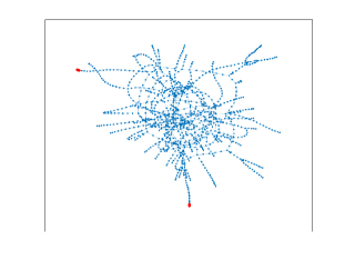
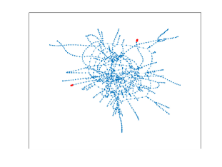
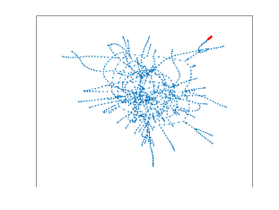
h!tb (a) (b) (c)

Figure 1: Example 4.2. The vertices (marked in red) that are connected by the edges to be removed in order to simplify the network according to ${\mathcal{E}}_{L_{f}}$ for (a), according to ${\widetilde{\mathcal{E}}}_{L_{f}}$ for (b), and according to ${\mathcal{E}}_{\rho}$ for (c).

Conversely, the largest entries of the edge importance vectors and the virtual edge importance vectors computed using (9) or (10) correspond to the same edges displayed in Table 5. Setting to zero the weights associated with the two highway segments Duisburg - Düsseldorf and München - Kirchheim (both in bold face in the first column of Table 5) results in the network ${\mathcal{G}}_{2}$, for which one has

$$T_{{\mathcal{G}}_{2}}=1.2108\cdot 10^{4};\;\;\;\;\frac{T_{\mathcal{G}}-T_{{\mathcal{G}}_{2}}}{T_{\mathcal{G}}}=3.6214\cdot 10^{-2},\;\;\;\;\;\;\;\;$$

while increasing by one the weights associated with the same edges results in the network ${\mathcal{G}}_{3}$, for which one has

$$T_{{\mathcal{G}}_{3}}=1.3359\cdot 10^{4};\;\;\;\;\frac{T_{{\mathcal{G}}_{3}}-T_{\mathcal{G}}}{T_{\mathcal{G}}}=6.3330\cdot 10^{-2}.\;\;\;\;\;\;\;\;$$

On the other hand, setting to one the (vanishing) entries of $A$ associated with the two virtual highway segments München - Duisburg and München - Hamburg (both in bold face in the second column of Table 5) returns the network ${\mathcal{G}}_{4}$ with

$$T_{{\mathcal{G}}_{4}}=1.3662\cdot 10^{4};\;\;\;\;\frac{T_{{\mathcal{G}}_{4}}-T_{\mathcal{G}}}{T_{\mathcal{G}}}=8.7477\cdot 10^{-2}.\;\;\;\;\;\;\;\;$$

As for Perron communicability in Autobahn, one has $P_{\mathcal{G}}=2.2448\cdot 10^{3}$. Although the graph ${\mathcal{G}}$ is irreducible, some entries of the Perron vector $x$ are close to machine precision. In particular, the edges to remove in order to simplify the network, that are associated with the two smallest entries of the Perron edge importance vector, are the final highway segments Wildsdruff - Wildeck and Wüstenbrand - Wommen, connecting the four vertices associated with such quasi-zero components of $x$ (see Figure 1(c)). This results in the (disconnected) network ${\mathcal{G}}_{5}$, for which we have

$$P_{{\mathcal{G}}_{5}}=2.2448\cdot 10^{3};\;\;\;\;\frac{P_{{\mathcal{G}}}-P_{{\mathcal{G}_{5}}}}{P_{\mathcal{G}}}=-4.8619\cdot 10^{-15};\;\;\;\;\;\;\;\;T_{{\mathcal{G}}_{5}}=1.2547\cdot 10^{4};\;\;\;\;\frac{T_{{\mathcal{G}}}-T_{{\mathcal{G}}_{5}}}{T_{\mathcal{G}}}=1.2521\cdot 10^{-3}.$$

So the simplification is slightly less satisfactory than that obtained in ${\mathcal{G}}_{1}$ or in ${\widetilde{\mathcal{G}}}_{1}$. Elimination of the edges associated with the two highway segments Duisburg - Düsseldorf and Essen - Duisburg (both in bold face in the first column of Table 6) returns the network ${\mathcal{G}}_{6}$, for which we

$$P_{{\mathcal{G}}_{6}}=1.2677\cdot 10^{3};\;\;\;\;\frac{P_{{\mathcal{G}}}-P_{{\mathcal{G}}_{6}}}{P_{\mathcal{G}}}=4.3527\cdot 10^{-1};\;\;\;\;\;\;\;\;T_{{\mathcal{G}}_{6}}=1.2155\cdot 10^{4};\;\;\;\;\frac{T_{{\mathcal{G}}}-T_{{\mathcal{G}}_{6}}}{T_{\mathcal{G}}}=3.2513\cdot 10^{-2}.$$

Again the decrease is less than that in ${\mathcal{G}}_{2}$. Conversely, increasing by one the weights associated with the same edges results in the network ${\mathcal{G}}_{7}$, for which one has

$$P_{{\mathcal{G}}_{7}}=2.5248\cdot 10^{3};\;\;\;\;\frac{P_{{\mathcal{G}}_{7}}-P_{{\mathcal{G}}}}{P_{\mathcal{G}}}=1.2472\cdot 10^{-2};\;\;\;\;\;\;\;\;T_{{\mathcal{G}}_{7}}=1.3480\cdot 10^{4};\;\;\;\;\frac{T_{{\mathcal{G}}_{7}}-T_{{\mathcal{G}}}}{T_{\mathcal{G}}}=7.2982\cdot 10^{-2}.$$

The increase in this case is greater than that in ${\mathcal{G}}_{3}$. Finally, setting to one the (vanishing) entries of $A$ associated with the two virtual highway segments Essen - Düsseldorf and Gelsenkirchen - Duisburg (both in bold face in the second column of Table 6) results in the network ${\mathcal{G}}_{8}$ with

$$P_{{\mathcal{G}}_{8}}=2.4892\cdot 10^{3};\;\;\;\;\frac{P_{{\mathcal{G}}_{8}}-P_{{\mathcal{G}}}}{P_{\mathcal{G}}}=1.0885\cdot 10^{-1};\;\;\;\;\;\;\;\;T_{{\mathcal{G}}_{8}}=1.3271\cdot 10^{4};\;\;\;\;\frac{T_{{\mathcal{G}}_{8}}-T_{{\mathcal{G}}}}{T_{\mathcal{G}}}=5.6327\cdot 10^{-2}.$$

Therefore the result is less satisfactory than that obtained for the network ${\mathcal{G}}_{4}$.

Notice that one has $\|\mathbf{W}|_{{\mathcal{A}}}\|_{F}=\sqrt{2}\|\mathbf{W}|_{{\mathcal{L}}}\|_{F}=5.1765\cdot 10^{-1}$.

${\mathcal{E}}_{L_{f}}$ [or ${\widetilde{\mathcal{E}}}_{L_{f}}$]	$e(v_{i}\leftrightarrow v_{j})$ associated with ${\mathcal{E}}_{L_{f}}$	$e(v_{i}\leftrightarrow v_{j})$ associated with ${\widetilde{\mathcal{E}}}_{L_{f}}$
$6.5794\cdot 10^{-4}$	Allershausen $\longleftrightarrow$ Allersberg	Wüstenbrand $\longleftrightarrow$ Wommen
$6.5794\cdot 10^{-4}$	Bünde $\longleftrightarrow$ Bissendorf	Thiendorf $\longleftrightarrow$ Teupitz
$6.5794\cdot 10^{-4}$	Zarrentin $\longleftrightarrow$ Witzhave	Zrbig $\longleftrightarrow$ Wiedemar
$6.5794\cdot 10^{-4}$	Wunsiedel $\longleftrightarrow$ Wolnzach	Zarrentin $\longleftrightarrow$ Witzhave
$6.5794\cdot 10^{-4}$	Thiendorf $\longleftrightarrow$ Teupitz	Aitrach $\longleftrightarrow$ Aichstetten
$6.5794\cdot 10^{-4}$	Wüstenbrand $\longleftrightarrow$ Wommen	Wesuwe $\longleftrightarrow$ Weener
$6.5794\cdot 10^{-4}$	Alsfeld $\longleftrightarrow$ Achern	Wunsiedel $\longleftrightarrow$ Wolnzach
$6.5794\cdot 10^{-4}$	Wesuwe $\longleftrightarrow$ Weener	Zwingenberg $\longleftrightarrow$ Zeppelinheim
$6.5794\cdot 10^{-4}$	Zwingenberg $\longleftrightarrow$ Zeppelinheim	Bünde $\longleftrightarrow$ Bissendorf
$6.5794\cdot 10^{-4}$	Zrbig $\longleftrightarrow$ Wiedemar	Alsfeld $\longleftrightarrow$ Achern

Table 4: Example 4.2. The first $10$ highway segments that could be removed, in order to reduce the complexity of Autobahn without changing the network communication significantly, according to determination of the edge importance based on gradient. The edges in the second and in the third column are determined using (9) and (10), respectively.

${\mathcal{E}}_{L_{f}}$	$e(v_{i}\leftrightarrow v_{j})$	${\widehat{\mathcal{E}}}_{L_{f}}$	$e(v_{i}\leftrightarrow v_{j})$
$2.1662\cdot 10^{-2}$	Duisburg $\longleftrightarrow$ Düsseldorf	$2.6669\cdot 10^{-2}$	München $\longleftrightarrow$ Duisburg
$1.9101\cdot 10^{-2}$	München $\longleftrightarrow$ Kirchheim	$2.5163\cdot 10^{-2}$	München $\longleftrightarrow$ Hamburg
$1.8792\cdot 10^{-2}$	Essen $\longleftrightarrow$ Duisburg	$2.3688\cdot 10^{-2}$	München $\longleftrightarrow$ Düsseldorf
$1.8106\cdot 10^{-2}$	Duisburg $\longleftrightarrow$ Dortmund	$2.3072\cdot 10^{-2}$	Hamburg $\longleftrightarrow$ Duisburg
$1.7092\cdot 10^{-2}$	Krefeld $\longleftrightarrow$ Duisburg	$2.1296\cdot 10^{-2}$	München $\longleftrightarrow$ Frankfurt
$1.6862\cdot 10^{-2}$	Hamburg $\longleftrightarrow$ Hagen	$2.0550\cdot 10^{-2}$	München $\longleftrightarrow$ Essen
$1.4823\cdot 10^{-2}$	Duisburg $\longleftrightarrow$ Dinslaken	$2.0448\cdot 10^{-2}$	Hamburg $\longleftrightarrow$ Düsseldorf
$1.4348\cdot 10^{-2}$	Gelsenkirchen $\longleftrightarrow$ Essen	$2.0325\cdot 10^{-2}$	München $\longleftrightarrow$ Gelsenkirchen
$1.4105\cdot 10^{-2}$	Flughafen $\longleftrightarrow$ Duisburg	$1.9993\cdot 10^{-2}$	München $\longleftrightarrow$ Groá
$1.3341\cdot 10^{-2}$	Hagen $\longleftrightarrow$ Groá	$1.9701\cdot 10^{-2}$	München $\longleftrightarrow$ Dortmund

Table 5: Example 4.2. The first $10$ highway segments that should be widened/narrowed, in order to increase/decrease the network communication in Autobahn (in the first column) and the first $10$ highway segments that should be built in order to increase the network communication in Autobahn (in the second column), according to the edge importance vector ${\mathcal{E}}_{L_{f}}$ and the virtual edge importance vector ${\widehat{\mathcal{E}}}_{L_{f}}$, respectively.

${\mathcal{E}}_{\rho}$	$e(v_{i}\leftrightarrow v_{j})$	${\widehat{\mathcal{E}}}_{\rho}$	$e(v_{i}\leftrightarrow v_{j})$
$3.2881\cdot 10^{-1}$	Duisburg $\longleftrightarrow$ Düsseldorf	$2.4476\cdot 10^{-1}$	Essen $\longleftrightarrow$ Düsseldorf
$2.9148\cdot 10^{-1}$	Essen $\longleftrightarrow$ Duisburg	$2.0210\cdot 10^{-1}$	Gelsenkirchen $\longleftrightarrow$ Duisburg
$2.2093\cdot 10^{-1}$	Duisburg $\longleftrightarrow$ Dinslaken	$1.8389\cdot 10^{-1}$	Düsseldorf $\longleftrightarrow$ Dortmund
$2.1899\cdot 10^{-1}$	Duisburg $\longleftrightarrow$ Dortmund	$1.6971\cdot 10^{-1}$	Gelsenkirchen $\longleftrightarrow$ Düsseldorf
$1.8552\cdot 10^{-1}$	Düsseldorf $\longleftrightarrow$ Dinslaken	$1.6446\cdot 10^{-1}$	Essen $\longleftrightarrow$ Dinslaken
$1.8126\cdot 10^{-1}$	Krefeld $\longleftrightarrow$ Duisburg	$1.6302\cdot 10^{-1}$	Essen $\longleftrightarrow$ Dortmund
$1.5044\cdot 10^{-1}$	Gelsenkirchen$\longleftrightarrow$ Essen	$1.6216\cdot 10^{-1}$	Elmpt $\longleftrightarrow$ Duisburg
$1.4553\cdot 10^{-1}$	Flughafen $\longleftrightarrow$ Duisburg	$1.5221\cdot 10^{-1}$	Krefeld $\longleftrightarrow$ Düsseldorf
$1.3617\cdot 10^{-1}$	Elmpt $\longleftrightarrow$ Düsseldorf	$1.3493\cdot 10^{-1}$	Krefeld $\longleftrightarrow$ Essen
$1.2071\cdot 10^{-1}$	Essen $\longleftrightarrow$ Elmpt	$1.3345\cdot 10^{-1}$	Eilsleben $\longleftrightarrow$ Duisburg

Table 6: Example 4.2. The first $10$ highway segments that should be widened/narrowed, in order to increase/decrease the network communication in Autobahn (in the first column) and the first $10$ highway segments that should be built in order to increase the network communication in Autobahn (in the second column), according to the Perron edge importance vector ${\mathcal{E}}_{\rho}$ and the Perron virtual edge importance vector ${\widehat{\mathcal{E}}}_{\rho}$, respectively.

EXAMPLE 4.3.

Consider the directed weighted graph $\mathcal{G}$ that represents the network C.elegans available at [28], i.e., the metabolic network of the Caenorhabditis elegans worm. The network contains $n=306$ vertices that represent neurons and $m=2345$ edges. Two neurons are connected if at least one synapse or gap junction exists between them and the associated edge-weight is the number of synapses and gap junctions. The network is disconnected.

The total communicability in (2) is $T_{\mathcal{G}}=3.3401\cdot 10^{6}$. The gradient $\nabla T_{\mathcal{G}}$ in (3) has been computed by evaluating the matrix $L_{f}(\mathbf{A}^{T},uv^{T})$ in (8) using (9). The total transmission is $\|\nabla T_{\mathcal{G}}\|_{2}=7.9032\cdot 10^{6}$. The gradient $\nabla T_{\mathcal{G}}$ has been approximated by evaluating $L_{f}(\mathbf{A}^{T},uv^{T})$ using (10) with $h=\frac{2}{n}\cdot 10^{-4}=6.5359\cdot 10^{-7}$, obtaining $\widetilde{\nabla T}_{\mathcal{G}}$. The resulting total transmission is $\|\widetilde{\nabla T}_{\mathcal{G}}\|_{2}=7.9032\cdot 10^{6}$, having

$$\frac{\|\nabla T_{\mathcal{G}}-\widetilde{\nabla T}_{\mathcal{G}}\|_{2}}{{\|\nabla T_{\mathcal{G}}}\|_{2}}=4.4914\cdot 10^{-9}.$$

As for both the edge importance vector ${\mathcal{E}}_{L_{f}}$ and the virtual edge importance vector $\widehat{\mathcal{E}}_{L_{f}}$, one obtains the same results, displayed in Table 7, regardless of whether $\nabla T_{\mathcal{G}}$ or $\widetilde{\nabla T}_{\mathcal{G}}$ is used.

Removing the two edges in bold face in the second column of Table 7, associated with the smallest entries of the edge importance results in the network ${\mathcal{G}}_{1}$ one obtains

$$T_{{\mathcal{G}}_{1}}=3.3401\cdot 10^{6};\;\;\;\;\frac{T_{\mathcal{G}}-T_{{\mathcal{G}}_{1}}}{T_{\mathcal{G}}}=5.9879\cdot 10^{-7}.$$

Setting to zero the weights associated with the two edges in bold face in the fourth column of Table 7) results in the network ${\mathcal{G}}_{2}$, for which one has

$$T_{{\mathcal{G}}_{2}}=2.9282\cdot 10^{6};\;\;\;\;\frac{T_{\mathcal{G}}-T_{{\mathcal{G}}_{2}}}{T_{\mathcal{G}}}=1.2332\cdot 10^{-1},\;\;\;\;\;\;\;\;$$

while increasing by one the weights associated with the same edges results in the network ${\mathcal{G}}_{3}$, for which one has

$$T_{{\mathcal{G}}_{3}}=3.8047\cdot 10^{6};\;\;\;\;\frac{T_{{\mathcal{G}}_{3}}-T_{\mathcal{G}}}{T_{\mathcal{G}}}=1.3909\cdot 10^{-1}.\;\;\;\;\;\;\;\;$$

Finally, setting to one the (vanishing) entries of $A$ associated with the two virtual edges in bold face in the sixth column of Table 7) returns the network ${\mathcal{G}}_{4}$, with

$$T_{{\mathcal{G}}_{4}}=7.3327\cdot 10^{6};\;\;\;\;\frac{T_{{\mathcal{G}}_{4}}-T_{\mathcal{G}}}{T_{\mathcal{G}}}=1.1954\cdot 10^{0}.\;\;\;\;\;\;\;\;$$

Turning to the network modifications based on Perron root sensitivity in C.elegans, one has $P_{\mathcal{G}}=9.1975\cdot 10^{5}$. The graph ${\mathcal{G}}$ is reducible, some entries of the Perron vector $x$ are vanishing. In particular, removing the edges in bold face in the second column of Table 8, which are associated with two vanishing entries of the Perron edge importance vector, results in the network ${\mathcal{G}}_{5}$, for which one has

$$P_{{\mathcal{G}}_{5}}=9.1931\cdot 10^{5};\;\;\;\;\frac{P_{{\mathcal{G}}}-P_{{\mathcal{G}_{5}}}}{P_{\mathcal{G}}}=4.7732\cdot 10^{-4};\;\;\;\;\;\;\;\;T_{{\mathcal{G}}_{5}}=3.3381\cdot 10^{6};\;\;\;\;\frac{T_{{\mathcal{G}}}-T_{{\mathcal{G}}_{5}}}{T_{\mathcal{G}}}=6.0666\cdot 10^{-4}.$$

So the simplification is less satisfactory than that obtained in ${\mathcal{G}}_{1}$. Elimination of the edges in bold face in the fourth column of Table 8) returns the network ${\mathcal{G}}_{6}$, for which one has

$$P_{{\mathcal{G}}_{6}}=7.4856\cdot 10^{5};\;\;\;\;\frac{P_{{\mathcal{G}}}-P_{{\mathcal{G}}_{6}}}{P_{\mathcal{G}}}=1.8613\cdot 10^{-1};\;\;\;\;\;\;\;\;T_{{\mathcal{G}}_{6}}=2.9298\cdot 10^{6};\;\;\;\;\frac{T_{{\mathcal{G}}}-T_{{\mathcal{G}}_{6}}}{T_{\mathcal{G}}}=1.2284\cdot 10^{-1}.$$

The decrease is less than that in ${\mathcal{G}}_{2}$. Conversely, increasing by one the weights associated with the same edges results in the network ${\mathcal{G}}_{7}$, for which one has

$$P_{{\mathcal{G}}_{7}}=1.1140\cdot 10^{6};\;\;\;\;\frac{P_{{\mathcal{G}}_{7}}-P_{{\mathcal{G}}}}{P_{\mathcal{G}}}=2.1122\cdot 10^{-1};\;\;\;\;\;\;\;\;T_{{\mathcal{G}}_{7}}=3.7933\cdot 10^{6};\;\;\;\;\frac{T_{{\mathcal{G}}_{7}}-T_{{\mathcal{G}}}}{T_{\mathcal{G}}}=1.3569\cdot 10^{-1}.$$

The increase is less than that in ${\mathcal{G}}_{3}$. Finally, setting to one the (vanishing) entries of $A$ associated with the two virtual edges in bold face in the sixth column of Table 8) results in the network ${\mathcal{G}}_{8}$, having

$$P_{{\mathcal{G}}_{8}}=3.5870\cdot 10^{6};\;\;\;\;\frac{P_{{\mathcal{G}}_{8}}-P_{{\mathcal{G}}}}{P_{\mathcal{G}}}=2.8999\cdot 10^{0};\;\;\;\;\;\;\;\;T_{{\mathcal{G}}_{8}}=7.3364\cdot 10^{6};\;\;\;\;\frac{T_{{\mathcal{G}}_{8}}-T_{{\mathcal{G}}}}{T_{\mathcal{G}}}=1.1965\cdot 10^{0}.$$

Therefore the result is more satisfactory than that obtained in the network ${\mathcal{G}}_{4}$. Notice that $\|\mathbf{W}|_{{\mathcal{A}}}\|_{F}=1.2817\cdot 10^{-1}$.

${\mathcal{E}}_{L_{f}}$	$e(v_{i}\to v_{j})$	${\mathcal{E}}_{L_{f}}$	$e(v_{i}\to v_{j})$	${\widehat{\mathcal{E}}}_{L_{f}}$	$e(v_{i}\to v_{j})$
$1.2653\cdot 10^{-7}$	$v_{53}\to v_{303}$	$2.8888\cdot 10^{-2}$	$v_{71}\to v_{217}$	$1.1107\cdot 10^{-1}$	$v_{305}$ $\to$ $v_{149}$
$1.2653\cdot 10^{-7}$	$v_{151}\to v_{305}$	$2.6446\cdot 10^{-2}$	$v_{72}\to v_{216}$	$1.0213\cdot 10^{-1}$	$v_{305}\to v_{219}$
$1.2653\cdot 10^{-7}$	$v_{191}$ $\to$ $v_{305}$	$2.5673\cdot 10^{-2}$	$v_{73}$ $\to$ $v_{178}$	$9.6897\cdot 10^{-2}$	$v_{305}$ $\to$ $v_{218}$
$1.2653\cdot 10^{-7}$	$v_{243}$ $\to$ $v_{305}$	$2.2681\cdot 10^{-2}$	$v_{72}$ $\to$ $v_{144}$	$8.9795\cdot 10^{-2}$	$v_{305}$ $\to$ $v_{216}$
$1.2653\cdot 10^{-7}$	$v_{259}$ $\to$ $v_{305}$	$2.1866\cdot 10^{-2}$	$v_{76}$ $\to$ $v_{217}$	$8.9722\cdot 10^{-2}$	$v_{305}$ $\to$ $v_{217}$
$1.2653\cdot 10^{-7}$	$v_{267}$ $\to$ $v_{305}$	$2.1271\cdot 10^{-2}$	$v_{78}$ $\to$ $v_{217}$	$8.9222\cdot 10^{-2}$	$v_{305}$ $\to$ $v_{178}$
$1.2653\cdot 10^{-7}$	$v_{291}$ $\to$ $v_{305}$	$2.0888\cdot 10^{-2}$	$v_{75}$ $\to$ $v_{216}$	$8.5450\cdot 10^{-2}$	$v_{305}$ $\to$ $v_{174}$
$1.2653\cdot 10^{-7}$	$v_{292}$ $\to$ $v_{305}$	$2.0012\cdot 10^{-2}$	$v_{77}$ $\to$ $v_{216}$	$8.2518\cdot 10^{-2}$	$v_{305}$ $\to$ $v_{81}$
$1.2653\cdot 10^{-7}$	$v_{293}$ $\to$ $v_{305}$	$1.9903\cdot 10^{-2}$	$v_{71}$ $\to$ $v_{47}$	$7.9914\cdot 10^{-2}$	$v_{305}$ $\to$ $v_{82}$
$1.2653\cdot 10^{-7}$	$v_{294}$ $\to$ $v_{305}$	$1.9752\cdot 10^{-2}$	$v_{71}$ $\to$ $v_{72}$	$7.7984\cdot 10^{-2}$	$v_{305}$ $\to$ $v_{198}$

Table 7: Example 4.3. The smallest entries of the edge importance vector and the relevant junctions that could be removed without changing the network communication in C.elegans significantly (displayed in the first two columns). The largest entries of the edge importance vector and the relevant junctions to increase/decrease in order to increase/decrease the network communication (in the third and fourth columns). The largest entries of the virtual edge importance vector and the relevant junctions to add in order to increase the communication in C.elegans (in the fifth and sixth columns).

${\mathcal{E}}_{\rho}$	$e(v_{i}\to v_{j})$	${\mathcal{E}}_{\rho}$	$e(v_{i}\to v_{j})$	${\widehat{\mathcal{E}}}_{\rho}$	$e(v_{i}\to v_{j})$
$0$	$v_{53}\to v_{1}$	$2.7208\cdot 10^{-2}$	$v_{73}\to v_{178}$	$1.3484\cdot 10^{-1}$	$v_{305}\to v_{149}$
$0$	$v_{11}\to v_{5}$	$2.4126\cdot 10^{-2}$	$v_{71}\to v_{217}$	$1.3000\cdot 10^{-1}$	$v_{305}\to v_{219}$
$0$	$v_{12}$ $\to$ $v_{6}$	$2.2348\cdot 10^{-2}$	$v_{72}$ $\to$ $v_{216}$	$1.2205\cdot 10^{-1}$	$v_{305}$ $\to$ $v_{218}$
$0$	$v_{11}$ $\to$ $v_{19}$	$2.0573\cdot 10^{-2}$	$v_{72}$ $\to$ $v_{144}$	$1.1067\cdot 10^{-1}$	$v_{305}$ $\to$ $v_{178}$
$0$	$v_{11}$ $\to$ $v_{23}$	$1.8951\cdot 10^{-2}$	$v_{76}$ $\to$ $v_{217}$	$1.0811\cdot 10^{-1}$	$v_{305}$ $\to$ $v_{174}$
$0$	$v_{12}$ $\to$ $v_{24}$	$1.8489\cdot 10^{-2}$	$v_{71}$ $\to$ $v_{47}$	$1.0128\cdot 10^{-1}$	$v_{305}$ $\to$ $v_{81}$
$0$	$v_{12}$ $\to$ $v_{25}$	$1.8419\cdot 10^{-2}$	$v_{75}$ $\to$ $v_{216}$	$9.7793\cdot 10^{-2}$	$v_{305}$ $\to$ $v_{82}$
$0$	$v_{8}$ $\to$ $v_{26}$	$1.7529\cdot 10^{-2}$	$v_{74}$ $\to$ $v_{177}$	$9.5414\cdot 10^{-2}$	$v_{305}$ $\to$ $v_{157}$
$0$	$v_{11}$ $\to$ $v_{26}$	$1.7392\cdot 10^{-2}$	$v_{216}$ $\to$ $v_{81}$	$8.7441\cdot 10^{-2}$	$v_{305}$ $\to$ $v_{216}$
$0$	$v_{12}$ $\to$ $v_{26}$	$1.7269\cdot 10^{-2}$	$v_{78}$ $\to$ $v_{217}$	$8.6713\cdot 10^{-2}$	$v_{305}$ $\to$ $v_{217}$

Table 8: Example 4.3. The smallest entries of the Perron edge importance vector and the relevant junctions that could be removed without changing the communication in C.elegans significantly (displayed in the first two columns). The largest entries of the Perron edge importance vector and the relevant junctions to increase/decrease in order to increase/decrease the network communication in C.elegans (in the third and fourth columns). The largest entries of the virtual Perron edge importance vector and the relevant junctions to add in order to increase the network communication (displayed in the fifth and sixth columns).

4.2 Large networks

EXAMPLE 4.4.

Consider the unweighted undirected graph $\mathcal{G}$ that represents the continental US road network Usroads-48. The graph $\mathcal{G}$, which is available at [28], has $n=126146$ vertices, which represent intersections and road endpoints. The $m=161950$ edges represent roads which connect the intersections and endpoints. We analyze the network Usroads-48 with the tools discussed in Subsections 2.2 and 3.2 for large networks.

We would like to determine approximations of the smallest and largest elements of $L_{f}(A,ee^{T})|_{\mathcal{L}}$ that correspond to edges that should be removed to simplify the network or whose edge-weight should be modified to increase or decrease the total communicability. Moreover, we would like to determine approximations of the smallest and largest elements of $L_{f}(A,ee^{T})|_{\widehat{\mathcal{L}}}$ that correspond to edges that should be added to increase total communicability. We first carry out $5$ steps of the symmetric Lanczos process, computing $\mathbf{V}_{5}$ and $\mathbf{T}_{5}$, and make use of the latter to construct both $\mathbf{X}_{5}$ in (17), thanks to (18), and

$${\tilde{\mathbf{X}}}_{5}=\frac{f(\mathbf{T}_{5}+hne_{1}e_{1}^{T})-f(\mathbf{T}_{5}-hne_{1}e_{1}^{T})}{2h},$$

with $h=\frac{2}{n}\cdot 10^{-4}$. Then, proceeding as discussed in Subsection 2.2, both the approaches give the same estimates. The smallest element of the approximate $L_{f}(A,ee^{T})|_{{\mathcal{L}}}$ is $9.7462\cdot 10^{-7}$ and is associated with edge $e(v_{123259}\leftrightarrow v_{123258})$ while its largest element is $1.5008\cdot 10^{1}$ and is associated with edge $e(v_{19694}\leftrightarrow v_{19186})$; the smallest element of the approximate $L_{f}(A,ee^{T})|_{\widehat{\mathcal{L}}}$ is $2.2047\cdot 10^{-9}$ and is associated with edge $e(v_{25416}\leftrightarrow v_{11651})$ while its largest element is $1.9380\cdot 10^{1}$ and is associated with edge $e(v_{58080}\leftrightarrow v_{1})$.

Turning to the the structured Perron communicability, one has $P_{\mathcal{G}}^{{\mathcal{A}}}=1.9138\cdot 10^{2}$. The smallest entries of the Perron edge importance vector ${\mathcal{E}}_{\rho}$ and the relevant edges are displayed in Table 9 in the first and second columns, while the largest entries of ${\mathcal{E}}_{\rho}$ and the relevant edges are shown in the third and fourth columns. In order to increase the network communication one should add edge $e(v_{44182}\leftrightarrow v_{44035})$, which is associated with the largest entry of the $\widehat{\mathcal{L}}$-analogue of the Wilkinson perturbation.

${\mathcal{E}}_{\rho}$	$e(v_{i}\leftrightarrow v_{j})$	${\mathcal{E}}_{\rho}$	$e(v_{i}\leftrightarrow v_{j})$
$1.2197\cdot 10^{-40}$	$v_{105751}\leftrightarrow v_{105743}$	$2.2346\cdot 10^{-1}$	$v_{44182}\leftrightarrow v_{44067}$
$3.3336\cdot 10^{-40}$	$v_{42664}\leftrightarrow v_{42479}$	$1.8605\cdot 10^{-1}$	$v_{44182}\leftrightarrow v_{44154}$
$5.0488\cdot 10^{-40}$	$v_{114032}$ $\leftrightarrow$ $v_{42664}$	$1.8090\cdot 10^{-1}$	$v_{44182}$ $\leftrightarrow$ $v_{44087}$
$7.3043\cdot 10^{-40}$	$v_{44150}$ $\leftrightarrow$ $v_{44015}$	$1.5882\cdot 10^{-1}$	$v_{44154}$ $\leftrightarrow$ $v_{44067}$
$8.8379\cdot 10^{-40}$	$v_{68387}$ $\leftrightarrow$ $v_{68213}$	$1.5443\cdot 10^{-1}$	$v_{44087}$ $\leftrightarrow$ $v_{44067}$
$1.0103\cdot 10^{-39}$	$v_{39830}$ $\leftrightarrow$ $v_{39787}$	$1.5077\cdot 10^{-1}$	$v_{44323}$ $\leftrightarrow$ $v_{44182}$
$1.0695\cdot 10^{-39}$	$v_{29088}$ $\leftrightarrow$ $v_{29056}$	$1.4155\cdot 10^{-1}$	$v_{44255}$ $\leftrightarrow$ $v_{44182}$
$1.2043\cdot 10^{-39}$	$v_{90123}$ $\leftrightarrow$ $v_{89379}$	$1.4099\cdot 10^{-1}$	$v_{44356}$ $\leftrightarrow$ $v_{44182}$
$1.2478\cdot 10^{-39}$	$v_{78533}$ $\leftrightarrow$ $v_{78388}$	$1.1663\cdot 10^{-1}$	$v_{44067}$ $\leftrightarrow$ $v_{44035}$
$1.2821\cdot 10^{-39}$	$v_{35630}$ $\leftrightarrow$ $v_{35115}$	$9.2663\cdot 10^{-2}$	$v_{44067}$ $\leftrightarrow$ $v_{44019}$

Table 9: Example 4.4. The smallest entries of the Perron edge importance vector and the edges associated with the roads that could be removed in order to reduce the complexity of the network without changing the communication in Usroads-48 significantly (displayed in the first two columns). The largest entries of the Perron edge importance vector and the edges associated with the first ten roads that should be widened/narrowed in order to increase/decrease the network communication the most (in the third and fourth columns).

Removing the two edges in bold face in the second column of Table 9, associated with the smallest entries of the edge importance results in the network ${\mathcal{G}}_{1}$, for which one has

$$P_{{\mathcal{G}}_{1}}^{{\mathcal{A}}}=1.9138\cdot 10^{2};\;\;\;\;\frac{P_{\mathcal{G}}^{{\mathcal{A}}}-P_{{\mathcal{G}}_{1}}^{{\mathcal{A}}}}{P_{\mathcal{G}}^{{\mathcal{A}}}}=1.4851\cdot 10^{-16}.$$

Setting to zero the weights associated with the two edges in bold face in the fourth column of Table 9) results in the network ${\mathcal{G}}_{2}$, having

$$P_{{\mathcal{G}}_{2}}^{{\mathcal{A}}}=1.7487\cdot 10^{2};\;\;\;\;\frac{P_{\mathcal{G}}^{{\mathcal{A}}}-P_{{\mathcal{G}}_{2}}^{{\mathcal{A}}}}{P_{\mathcal{G}}^{{\mathcal{A}}}}=8.6228\cdot 10^{-2},$$

while increasing by one the weights associated with the same edges results in the network ${\mathcal{G}}_{3}$, for which one has

$$P_{{\mathcal{G}}_{3}}^{{\mathcal{A}}}=3.6445\cdot 10^{2};\;\;\;\;\frac{P_{{\mathcal{G}}_{3}}^{{\mathcal{A}}}-P_{\mathcal{G}}^{{\mathcal{A}}}}{P_{\mathcal{G}}^{{\mathcal{A}}}}=9.0435\cdot 10^{-1}.$$

Finally, setting to one the (vanishing) entry $w_{44182,44035}$ of the adjacency matrix $\mathbf{A}$ associated with the virtual edge $e(v_{44182}\leftrightarrow v_{44035})$ returns the network ${\mathcal{G}}_{4}$, with

$$P_{{\mathcal{G}}_{4}}^{{\mathcal{A}}}=2.4540\cdot 10^{2};\;\;\;\;\frac{P_{{\mathcal{G}}_{4}}^{{\mathcal{A}}}-P_{\mathcal{G}}^{{\mathcal{A}}}}{P_{\mathcal{G}}^{{\mathcal{A}}}}=2.8228\cdot 10^{-1}.$$

Notice that one has $\|\mathbf{W}|_{{\mathcal{A}}}\|_{F}=\sqrt{2}\|\mathbf{W}|_{{\mathcal{L}}}\|_{F}=2.9318\cdot 10^{-1}$.

5 Conclusion and comments on related work

The identification of important and unimportant edges is a fundamental problem in network analysis. Several techniques for this purpose have been described in the literature; see, e.g., [7, 8, 5, 10, 21, 22]. In [4] the authors propose a method that uses the gradient of the total communicability, and Schweitzer [27] recently described how the computational effort required by this method can be reduced. Section 2 of this paper reviews this method and discusses computational aspects when this technique is applied to small and medium-sized networks, as well as to large-scale networks. In particular, further ways to speed up the computations when the method is applied to large-scale networks are described.

Another approach to identify important and unimportant edges is to determine edge weights whose modification yields a relatively large change in the Perron root of the adjacency matrix. This is described in [10, 21]. The computations required are quite straightforward and the method discussed in the latter reference is easy to implement also for large-scale problems. We therefore are interest in whether modifications of the weights of the edges identified by this technique give a relatively large change in the total communicability. Section 3 reviews the method described in [21] and extends it to include edge removal. Computed examples reported in Section 4 show that, indeed, modifications of edge weights identified by the technique discussed in [21] yield relatively large changes in the total communicability.

References

- [1] F. Arrigo and M. Benzi, Edge modification criteria for enhancing the communicability of digraphs. SIAM J. Matrix Analysis Appl., 37 (2016), pp. 443–468.
- [2] F. Arrigo and F. Durastante, Mittag-Leffler functions and their applications in network science, SIAM J. Matrix Anal. Appl., 42 (2021), pp. 1581–1601.
- [3] M. Benzi and C. Klymko, Total communicability as a centrality measure, J. Complex Netw., 1 (2013), pp. 124–149.
- [4] O. De la Cruz Cabrera, J. Jin, S. Noschese, and L. Reichel, Communication in complex networks, Appl. Numer. Math., 172 (2022), pp. 186–205.
- [5] O. De la Cruz Cabrera, J. Jin, and L. Reichel, Sparse approximation of complex networks, Appl. Numer. Math., in press.
- [6] O. De la Cruz Cabrera, M. Matar, and L. Reichel, Analysis of directed networks via the matrix exponential, J. Comput. Appl. Math., 355 (2019), pp. 182–192.
- [7] O. De la Cruz Cabrera, M. Matar, and L. Reichel, Edge importance in a network via line graphs and the matrix exponential, Numer. Algorithms, 83 (2020), pp. 807–832.
- [8] O. De la Cruz Cabrera, M. Matar, and L. Reichel, Centrality measures for node-weighted networks via line graphs and the matrix exponential, Numer. Algorithms, 88 (2021), pp. 583–614.
- [9] Dynamic Connectome Lab - Data Sets. https://sites.google.com/view/dynamicconnectomelab
- [10] S. El-Halouy, S. Noschese, and L. Reichel, Perron communicability and sensitivity of multilayer networks, Numer. Algorithms, 92 (2023), pp. 597–617.
- [11] E. Estrada, The Structure of Complex Networks: Theory and Applications, Oxford University Press, Oxford, 2011.
- [12] E. Estrada and D. J. Higham, Network properties revealed through matrix functions, SIAM Rev., 52 (2010), pp. 696–714.
- [13] E. Estrada and J. A. Rodriguez-Velazquez, Subgraph centrality in complex networks, Phys. Rev. E, 71 (2005), Art. 056103.
- [14] C. Fenu, D. Martin, L. Reichel, and G. Rodriguez, Network analysis via partial spectral factorization and Gauss quadrature, SIAM J. Sci. Comput., 35 (2013), pp. A2046–A2068.
- [15] N. J. Higham, Functions of Matrices: Theory and Computation, SIAM, Philadelphia, 2008.
- [16] P. Kandolf, A. Koskela, S. D. Relton, and M. Schweitzer, Computing low-rank approximations of the Fréchet derivative of a matrix function using Krylov subspace methods, Numer. Linear Algebra Appl., 28 (2021), Art. 2401.
- [17] S. Massei and F. Tudisco, Optimizing network robustness via Krylov subspaces, https://arxiv.org/pdf/2303.04971.pdf
- [18] A. Milanese, J. Sun, and T. Nishikawa, Approximating spectral impact of structural perturbations in large networks, Phys. Rev. E, 81 (2010), Art. 046112.
- [19] M. E. J. Newman, Networks: An Introduction, Oxford University Press, Oxford, 2010.
- [20] S. Noschese and L. Pasquini, Eigenvalue condition numbers: Zero-structured versus traditional, J. Comput. Appl. Math., 185 (2006), pp. 174–189.
- [21] S. Noschese and L. Reichel, Estimating and increasing the structural robustness of a network, Numer. Linear Algebra Appl., 29 (2022), Art. e2418.
- [22] S. Noschese and L. Reichel, Network analysis with the aid of the path length matrix, Numer. Algorithms, 95 (2024) pp. 451–470.
- [23] A. Ruhe, The two-sided Arnoldi algorithm for nonsymmetric eigenvalue problems, Matrix Pencils, eds. B. Kågström and A. Ruhe, Lecture Notes in Mathematics #973, Springer, Berlin, 1983, pp. 104–120.
- [24] P. Ruiz, J. Sastre, J. Ibáñez, and E. Defez, High performance computing of the matrix exponential, J. Comput. Appl. Math., 291 (2016), pp. 370–379.
- [25] Y. Saad, Numerical Methods for Large Eigenvalue Problems, revised ed., SIAM, Philadelphis, 2011.
- [26] Y. Saad, Iterative Methods for Sparse Linear Systems, 2nd ed., SIAM, Philadelphia, 2003.
- [27] M. Schweitzer, Sensitivity of matrix function based network communicability measures: Computational methods and a priori bounds, SIAM J. Matrix Anal. Appl., 44 (2023), pp. 1321–1348.
- [28] SuiteSparse Matrix Collection, https://sparse.tamu.edu.
- [29] J. H. Wilkinson, Sensitivity of eigenvalues II, Util. Math., 30 (1986), pp. 243–286.
- [30] S. Xu and F. Xue, Inexact rational Krylov subspace methods for approximating the action of functions of matrices, Electron. Trans. Numer. Anal., 58 (2023), pp. 538–567.
- [31] I. N. Zwaan and M. E. Hochstenbach, Krylov–Schur-type restarts for the two-sided Arnoldi method, SIAM J. Matrix Anal. Appl., 38 (2017), pp. 297–321.