Universal resonancelike emergence of chaos in complex networks of damped-driven nonlinear systems

Abstract

Characterizing the emergence of chaotic dynamics of complex networks is an essential task in nonlinear science with potential important applications in many fields such as neural control engineering, microgrid technologies, and ecological networks. Here, we solve a critical outstanding problem in this multidisciplinary research field: The emergence and persistence of spatio-temporal chaos in complex networks of damped-driven nonlinear oscillators in the significant weak-coupling regime, while they exhibit regular behavior when uncoupled. By developing a comprehensive theory with the aid of standard analytical methods, a hierarchy of lower-dimensional effective models, and extensive numerical simulations, we uncover and characterize the basic physical mechanisms concerning both heterogeneity-induced and impulse-induced emergence, enhancement, and suppression of chaos in starlike and scale-free networks of periodically driven, dissipative nonlinear oscillators.

Introduction.$-$Controlling the dynamical state of a complex network is a fundamental problem in science [1-5] with many potential applications, including neuronal [6] and ecological [7] networks. While most of these works consider networks of linear systems [2,5], only lately has the generic and richer case of networks of nonlinear systems [1,4] started to be investigated. Also, the majority of studies of coupled nonlinear systems subjected to external excitations focused on either local (homogeneous) diffusive-type or global (all-to-all) coupling. However, little attention has been paid to the possible influences of a heterogeneous connectivity on both the emergence and strength of chaos in complex networks of nonautonomous nonlinear systems. Here we characterize the emergence and persistence (in parameter space) of chaos in heterogeneous networks of damped-driven nonlinear systems when the complex network presents a non-chaotic state in the absence of coupling, while a stable chaotic state emerges after coupling the same nonautonomous nodes. Specifically, we study the interplay among heterogeneous connectivity, driving period, and impulse transmitted by a homogeneous (non-harmonic) periodic excitation in the emergence and persistence of spatio-temporal chaos in complex networks in the significant weak-coupling regime. For the sake of clarity, the findings are discussed through the analysis of starlike networks (SNs) of $N+1$ damped-driven two-well Duffing oscillators. This system is sufficiently simple to obtain analytical predictions while retaining the universal features of a dissipative chaotic system. The complete model system reads

$$\overset{..}{x}_{H} =\left(1-\lambda N\right)x_{H}-x_{H}^{3}-\delta\overset{.}{x}_{H}+\gamma f\left(t\right)+\lambda\sum_{i=1}^{N}y_{i},$$

$$\overset{..}{y}_{i} =\left(1-\lambda\right)y_{i}-y_{i}^{3}-\delta\overset{.}{y}_{i}+\gamma f\left(t\right)+\lambda x_{H},$$ (1)

$i=1,...,N$, where $f(t)$ is a unit-amplitude $T$-periodic excitation and $\lambda$ is the coupling. These equations describe the dynamics of a highly connected node (or hub), $x_{H}$, and $N$ linked oscillators (or leaves), $y_{i}$. For concreteness, we shall consider the elliptic excitation $f(t)=f_{ellip}(t)\equiv$ $A(m)\operatorname{sn}(4Kt/T)\operatorname*{dn}\left(4Kt/T\right)$ [8] (see Fig. 1(a) and Supplemental Material (SM) [9] for a detailed characterization of $f_{ellip}(t)$). In this Letter, we concentrate on the relevant (typically asynchronous) case of sufficiently small coupling, $\lambda$, external excitation amplitude, $\gamma$, and damping coefficient, $\delta$, such that the dynamics of the leaves may be decoupled from that of the hub on the one hand, and may be suitably described as a periodic orbit around one of the potential minima on the other. Specifically, we assume $\lambda=O\left(\gamma^{2}\right)$ throughout this work.

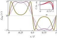
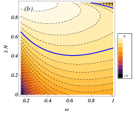
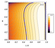
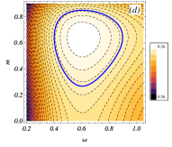
Figure 1: (a) External excitation $f_{ellip}(t)=$ $A(m)\operatorname{sn}(4Kt/T)\operatorname*{dn}\left(4Kt/T\right)$ vs $t/T$, where $T$ is the period and $A(m)\equiv 1/\left\{a+b/\left[1+\exp\left(\left\{m-c\right\}/d\right)\right]\right\}$, with $a\equiv 0.43932$, $b\equiv 0.69796$, $c\equiv 0.3727$, and $d\equiv 0.26883$, for three values of the shape parameter: $m=0$ (sinusoidal pulse), $m=0.72\simeq m_{\max}$ (nearly square-wave pulse), and $m=0.999$ (double-humped pulse). Inset: The normalized impulse $I\left(m\right)/I\left(m=0\right)$ (solid line) and the Fourier coefficient $a_{0}(m)$ (dashed line; see the text). Chaotic threshold function $U\left(\omega,\lambda N,m\right)$ [cf. Eq.(7)] vs (b) $\omega$ and $\lambda N$ for $m=0.65\simeq m_{\max}^{a_{0}}$, (c) $\lambda N$ and $m$ for $\omega=0.65$, and (d) $\omega$ and $m$ for $\lambda N=0.45$. The solid blue lines indicate the chaotic boundary corresponding to $\gamma/\delta=0.29$ [cf. Eq.(7)].

Effective model.$-$Equations (1) for the leaves become

$$\overset{..}{y}_{i}=y_{i}-y_{i}^{3}-\delta\overset{.}{y}_{i}+\gamma f_{ellip}\left(t\right),$$ (2)

$i=1,...,N$. After using the properties of the Fourier series of $f_{ellip}\left(t\right)$ (see SM [9] for analytical details) and applying standard perturbation methods [10] for the main resonance case, one obtains

$$y_{i}\left(t\rightarrow\infty\right)\sim\xi_{i}+\frac{\gamma a_{0}\left(m\right)}{2-\omega^{2}}\sin\left(\omega t\right),$$ (3)

where $\omega\equiv 2\pi/T$, $\xi_{i}=\pm 1$ depending on the initial conditions, while the first Fourier coefficient of $f_{ellip}\left(t\right)$, $a_{0}\left(m\right)$, presents a single maximum at $m=m_{\max}^{a_{0}}\simeq 0.65$ [see Fig 1(a), inset]. Since the initial conditions are randomly chosen, this means that the quantities $\xi_{i}$ behave as discrete random variables governed by Rademacher distributions. After inserting Eq. (3) into Eq. (1), the resulting equation for the hub reads

$$\overset{..}{x}_{H}=\left(1-\lambda N\right)x_{H}-x_{H}^{3}-\delta\overset{.}{x}_{H}+\Gamma\sin(\omega t)+\lambda\Xi,$$ (4)

where $\Xi\equiv\sum_{i=1}^{N}\xi_{i}$,$\ \Gamma\equiv\gamma a_{0}\left(m\right)\left[1+\lambda N/\left(2-\omega^{2}\right)\right]+O\left(\gamma^{3}a_{0}^{2}\left(m\right)\right)$. For finite $N$, the quantity $\Xi$ behaves as a discrete random variable governed by a binomial distribution with zero mean and variance $N$, while for sufficiently large $N$ one may assume that $\Xi$ behaves as a continuous random variable governed by a normal distribution. Although the hub’s dynamics are generally affected by spatial quenched disorder through the term $\lambda\Xi$, one expects that it may be neglected in the present case of weak coupling (WC) $\left(1\gg\lambda\gtrsim 0\right)$ according to the above assumptions (see SM [9] for a comparison of the cases with and without the term $\lambda\Xi$). Thus, the network described by Eq. (1) can be effectively replaced by a hierarchy of reduced networks in which a hub is coupled to $M$ effective leaves, each of which represents $n_{j}$ randomly chosen identical leaves (i.e., leaves having exactly the same initial conditions) such that the condition $\sum_{j=1}^{M}n_{j}=N$ is satisfied, in the WC regime and for values of $m$ sufficiently less than $1$:

$$\overset{..}{x}_{H} =\left(1-\lambda N\right)x_{H}-x_{H}^{3}-\delta\overset{.}{x}_{H}+\gamma a_{0}(m)\sin\left(\omega t\right)$$

$$+\lambda\sum_{j=1}^{M}n_{j}y_{L,j},$$

$$\overset{..}{y}_{L,j} =\left(1-\lambda\right)y_{L,j}-y_{L,j}^{3}-\delta\overset{.}{y}_{L,j}+\gamma a_{0}(m)\sin\left(\omega t\right)+\lambda x_{H},$$ (5)

$j=1,...,M$, where $y_{L,j}$ represents the common leaf associated with each group (cluster) of identical leaves. Equation (4) indicates that the possibility of heterogeneity-induced emergence of chaos in the hub’s dynamics is now expected from the lowering of the potential barrier’s height $h\equiv\left(1-\lambda N\right)^{2}/4$ as $N$ is increased on the one hand, and the presence of the additional resonant excitation $\gamma a_{0}\left(m\right)\lambda\left[N/\left(2-\omega^{2}\right)\right]\sin\left(\omega t\right)$ on the other. Notice that the amplitude of this coupling-induced resonant excitation effectively depends upon the impulse transmitted by $f_{ellip}\left(t\right)$ through the Fourier coefficient $a_{0}\left(m\right)$. Quantitatively, this expectation can be deduced with the aid of the Melnikov method (MM) [11,12]. Indeed, the application of MM to Eq. (2) provides an estimate of a necessary condition for the emergence of chaos:

$$\frac{\gamma}{\delta}\geqslant U\left(\omega,\lambda N=0,m\right)\equiv\frac{2\sqrt{2}\cosh\left(\pi\omega/2\right)}{3\pi\omega a_{0}(m)},$$ (6)

where $U\left(\omega,\lambda N,m\right)$ is the chaotic threshold function. Assuming that $N$ satisfies the condition $0<\lambda N<1$ in order to preserve the existence of an underlying separatrix for all $N$, the application of MM to Eq. (4) after dropping the term $\lambda\Xi=O\left(\gamma^{2}\right)$ provides an estimate of the corresponding necessary condition for the emergence of chaos:

$$\frac{\gamma}{\delta}\geqslant U\left(\omega,\lambda N,m\right)\equiv\frac{2\sqrt{2}\left(1-\lambda N\right)^{3/2}\cosh\left(\frac{\pi\omega}{2\sqrt{1-\lambda N}}\right)}{3\pi\omega a_{0}(m)\left(1+\frac{\lambda N}{2-\omega^{2}}\right)}$$ (7)

(see SM [9] for a derivation of Eqs. (6) and (7)). Now, the following remarks may be in order. First, the chaotic threshold function for the hub, Eq. (7), reduces to that of the leaves, Eq. (6), when $\lambda N\rightarrow 0$, i.e., for the limiting case of isolated nodes $\left(\lambda=0\right)$ and, in the present WC regime, for the limiting case of homogeneous connectivity $\left(N=1\right)$, as expected. Second, having fixed the ratio $\gamma/\delta$ and the coupling $\lambda$, the possibility of chaotic behaviour is predicted to be greater for the hub than for the leaves over wide ranges of $\omega$, while this difference strongly depends on $N$ [cf. Eqs. (6) and (7); see Fig. 1(b)]. Third, having fixed the coupling $\lambda$ and the angular frequency $\omega$, the chaotic threshold function presents a single minimum in the $\lambda N-m$ parameter plane at $N=N_{\min}\equiv N_{\min}(\omega)$ and $m=m_{\min}\simeq m_{\max}^{a_{0}}\simeq 0.65$ (irrespective of the driving period), which means that the possibility of chaotic behaviour is predicted to be higher when the impulse transmitted is maximum and for intermediate values of $\lambda N$ than for the limiting cases $\lambda N\rightarrow 0,1$ [cf. Eq. (7); see Fig. 1(c)]. And fourth, having fixed the coupling $\lambda$ and the number of leaves $N$, the chaotic threshold function presents a single minimum in the $\omega-m$ parameter plane at $\omega=\omega_{\min}\equiv\omega_{\min}(N)$ and $m=m_{\min}\simeq m_{\max}^{a_{0}}\simeq 0.65$ (irrespective of the driving period), which means again that the possibility of chaotic behaviour is predicted to be greater when the impulse transmitted is maximum and for intermediate values of $\omega$ than for the limiting cases $\omega\rightarrow 0,\infty$ [cf. Eq. (7); see Fig. 1(d)]. Therefore, depending on the remaining parameters, one could expect a heterogeneity-induced (impulse-induced) route to chaos starting from a regular SN with a few leaves (low-impulse excitation) by solely increasing their number (the excitation impulse) on the one hand, and a heterogeneity-induced (impulse-induced) route to regularity starting from a chaotic SN with many leaves (high-impulse excitation) by further increasing (decreasing) their number (excitation impulse) on the other.

Extensive numerical simulations of the complete system [Eq. (1)] and the effective model system [Eq. (5)] confirmed an overall good agreement with these expectations even for quite small values of $M$. Specifically, one can compare the theoretical predictions and Lyapunov exponent (LE) calculations [14] of both systems [Eqs. (1) and (5)] [15]. Illustrative examples are shown in Figs. 2 and 3 for $N=138$ and values of $\delta,\gamma$ that are clearly beyond the perturbative regime (compare Figs. 1(b), 1(c), 1(d) with Figs. 2(b), 2(a), 2(c), respectively).

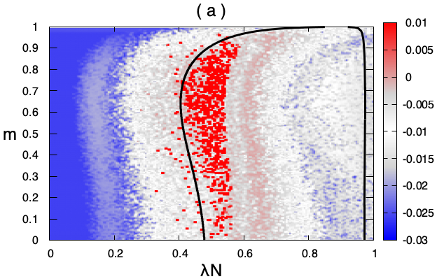
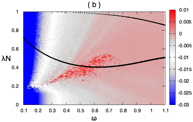
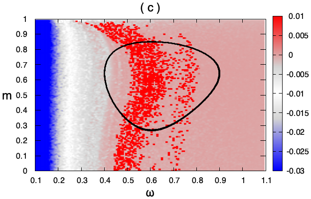
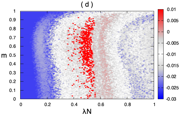
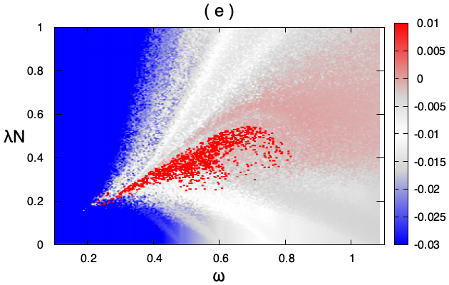
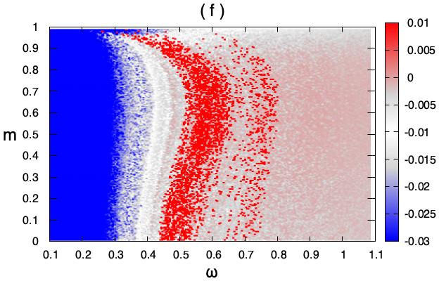
Figure 2: Maximal LE distribution in the (a), (d) $\lambda N-m$, (b), (e) $\omega-\lambda N$, and (c),(f) $\omega-m$ parameter planes for (a), (b), (c) the complete system [Eq. (1)] and (d), (e), (f) the effective model system [Eq. (5) with $M=138$, $n_{j}=1$, $j=1,...,138$] for (a), (d) $\omega=0.65$, (b), (e) $m=0.65\simeq m_{\max}^{a_{0}}$, and (c), (f) $\lambda=0.00326$. Fixed parameters: $N=138,\gamma=0.29,\delta=1$. The black lines indicate the chaotic boundary corresponding to $\gamma/\delta=0.29$ [cf. Eq.(7)].

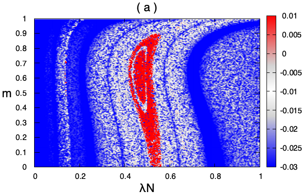
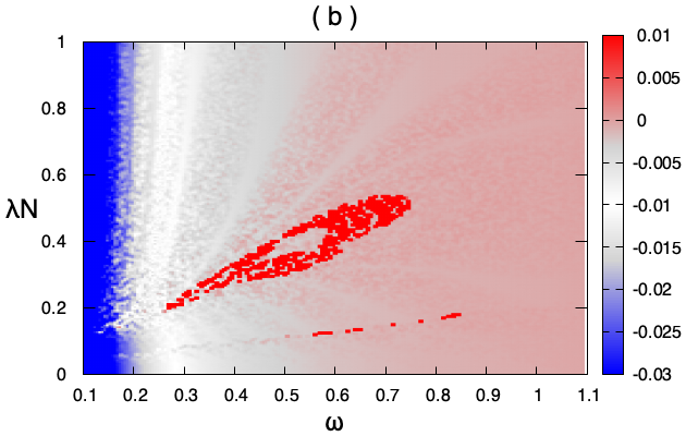
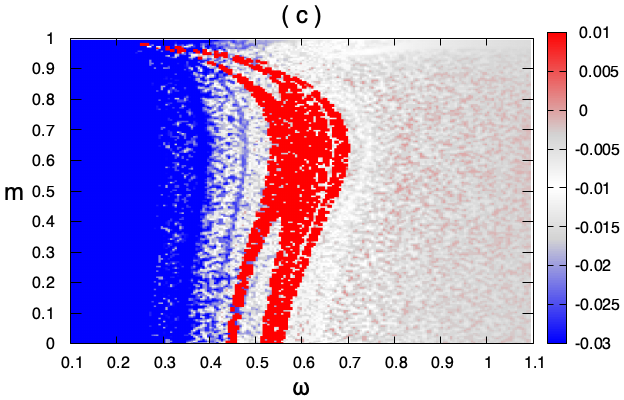
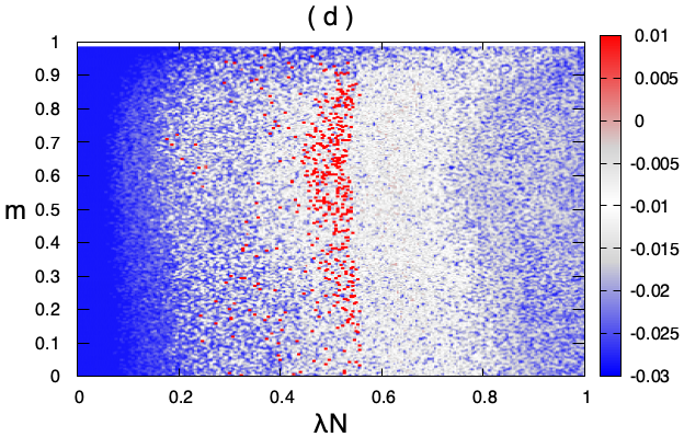
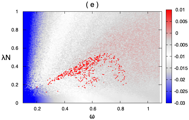
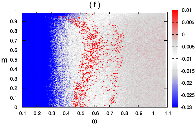
Figure 3: Maximal LE distribution in the (a), (d) $\lambda N-m$, (b), (e) $\omega-\lambda N$, and (c),(f) $\omega-m$ parameter planes for the effective model system [Eq. (5)] for (a), (d) $\omega=0.65$, (b), (e) $m=0.65\simeq m_{\max}^{a_{0}}$, (c), (f) $\lambda=0.00326$, and two values of the number of effective leaves: (a), (b), (c) $M=2$ and (d), (e), (f) $M=24$. The values of $n_{j}$ were randomly chosen while $\sum_{j=1}^{M}n_{j}=N$. Fixed parameters as in Fig. 2.

Typically, one finds for both systems [Eqs. (1) and (5)] a similar resonancelike emergence of chaos in the $\lambda N-m$, $\omega-\lambda N$, and $\omega-m$ parameter planes, which in its turn confirmed the effectiveness of model Eq. (5), as is clearly seen when comparing Figs. 2(a), 2(b), 2(c) with Figs. 2(d), 2(e), 2(f), respectively. As expected, the extent of the chaotic regions is smaller in the case of the harmonic approximation $a_{0}(m)\sin\left(\omega t\right)$, which is due to the absence of the effects of higher harmonics of $f_{ellip}\left(t\right)$. Remarkably, we found that the emergence of chaos is attenuated and slightly distorted in the parameter planes by decreasing the number $M$ of effective leaves from $M=N$, as for the case $M=24$ shown in Figs. 3(d), 3(e), 3(f). This suppressory effect occurs because the uniform initial randomness of the SN for $M=N$ is broken as $M$ decreases from $N$ due to the formation of clusters of identical leaves of different cardinality, giving rise to an increase in network desynchronization [16] which in turn makes it difficult to reach a synchronized chaotic state. But, on restoring the uniformity of the initial randomness, an increase in chaotic behaviour is observed even for quite small values of $M$, such as for $M=2$ in which we took $n_{1}=n_{2}$ [cf. Figs. 3(a), 3(b), 3(c)].

Scale-free networks.$-$Next, we discuss the possibility of extending the results obtained for an SN to Barabási-Albert (BA) networks [17] of the same Duffing oscillators. The system is given by

$$\overset{..}{x}_{i}=x_{i}-x_{i}^{3}-\delta\overset{.}{x}_{i}+\gamma f_{ellip}\left(t\right)-\lambda L_{ij}x_{j},$$ (8)

$\ i=1,...,N$, where $L_{ij}=\kappa_{i}\delta_{ij}-A_{ij}$ is the Laplacian matrix of the network, $\kappa_{i}=\sum_{j}A_{ij}$ is the degree of node $i$, and $A_{ij}$ is the adjacency matrix with entries of $1$ if $i$ is connected to $j$ and $0$ otherwise. Since in a BA network a highly connected node can be thought of as a hub of a local SN with a certain degree $\kappa$ picked up from the degree distribution ($P(\kappa)\sim\kappa^{-\alpha}$), one could expect the above scenario for SNs to remain valid to some degree. Indeed, for each hub with a sufficiently high (depending on the remaining parameters) degree $\kappa_{i}$, one systematically observes that the bifurcation diagram of its velocity $\overset{.}{x}_{i}$ vs coupling $\lambda$ presents, essentially, the same overall chaotic window over the range $0<\lambda\kappa_{i}<1$, in accordance with the predictions from the above SN scenario (see Figs. 4(b)). This is reflected in both the global chaos of the BA network, as shown in Fig. 4(a), and the number of chaotic nodes of the network, $N_{chaos}$, as shown in Fig. 4(c). When $\lambda\kappa_{i}\geqslant 1$, the potential associated with each hub of degree $\kappa_{i}$ undergoes a topological change, thus preventing the emergence of homoclinic chaos in such a hub. Therefore, for $\lambda$ values sufficiently far from the WC regime, the emergence of chaos in the BA network is no longer possible, as is confirmed by LE calculations (see Fig. 4(c) and SM [9] for additional examples).

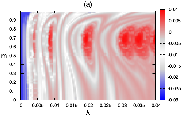
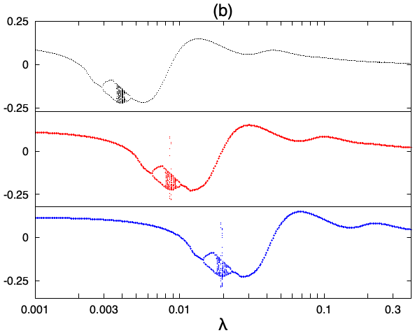
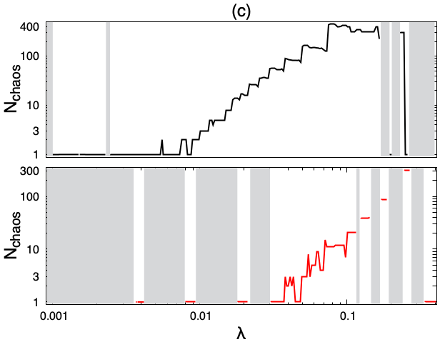
Figure 4: (a) Maximal LE distribution in the $\lambda-m$ parameter plane for a scale-free network [Eq. (8)] with $N=500,\alpha=2.7$, $\gamma=0.29,\delta=1,T=2\pi/0.65$. (b) Bifurcation diagrams for the velocities $\overset{.}{x}_{i}$ of its three main hubs ($\kappa_{1}=138$, $\kappa_{2}=61$, $\kappa_{3}=27$, from top to bottom) vs coupling $\lambda$ (logarithmic scale) for $m=0.65\simeq m_{\max}^{a_{0}}$. (c) Number of chaotic nodes $N_{chaos}$ (logarithmic scale) vs coupling $\lambda$ (logarithmic scale) for two sets of parameters $\left(\gamma,\delta,T\right)$: $(0.2,0.154,2\pi/0.5)$ (top) and ($0.29,1,2\pi/0.65)$ (bottom), and the remaining parameters as in (a) (grey regions denote $N_{chaos}=0$).

Conclusion.$-$Basic physical mechanisms have been discussed concerning both heterogeneity-induced and impulse-induced emergence, enhancement, and suppression of chaos in complex networks of periodically driven, dissipative nonlinear systems in the significant weak-coupling regime. With the aid of a hierarchy of lower-dimensional effective models and extensive numerical simulations, we have characterized the resonancelike interplay among heterogeneous connectivity, impulse transmitted by a homogeneous periodic excitation, and its driving period in the emergence and persistence of spatio-temporal chaos in starlike and scale-free networks of bistable oscillators. In view of the simplicity and generality of this multiple resonancelike scenario and the great robustness and scope of the physical mechanisms involved, we expect it to be quite readily testable by experiment, for instance in the context of nonlinear electronic circuits. Finally, we hope our results can serve as an important step towards understanding emergence of chaos in complex networks of interconnected damped-driven nonlinear systems in the case of time-varying connections [18], while the exploration of both the effectiveness of local application of additional chaos-suppressing excitations and of the effects of different coupling functions [19] represent exciting next steps for future research.

- (1) Y.-Y. Liu and A.-L. Barabási, Rev. Mod. Phys. 88, 035006 (2016).
- (2) T. Nepusz and T. Vicsek, Nat. Phys. 8, 568 (2012).
- (3) M. Pósfai, Y.-Y. Liu, J.-J. Slotine, and A.-L. Barabási, Sci. Rep. 3, 1067 (2013).
- (4) S. P. Cornelius, W. L. Kath, and A. E. Motter, Nat. Commun. 4, 1942 (2013); I. Klickstein, A. Shirin, and F. Sorrentino, Phys. Rev. Lett. 119, 268301 (2017).
- (5) G. Menichetti, L. Dall’Asta, and G. Bianconi, Phys. Rev. Lett. 113, 078701 (2014); Y. Zou, R. V. Donner, N. Marwan, J. F. Donges, and J. Kurths, Phys. Rep. 787, 1-97 (2019).
- (6) R. Laje and D. V. Buonomano, Nat. Neurosci. 16, 925 (2013); E. Tang and D. S. Bassett, Rev. Mod. Phys. 90, 031003 (2018).
- (7) M. Pascual and J. Dunne, Ecological Networks: Linking Structures to Dynamics in Food Webs (Oxford University Press, Oxford, 2006).
- (8) P. F. Byrd and M. D. Friedman, Handbook of Elliptic Integrals for Engineers and Scientists (Springer, Berlin, 1971).
- (9) See Supplemental Material at XXX for additional analytical details and numerical simulations.
- (10) C. Holmes and P. Holmes, J. Sound Vib. 78, 161 (1981).
- (11) V. K. Melnikov, Trans. Moscow Math. Soc. 12, 1 (1963) [Tr. Mosk. Ova. 12, 3 (1963)].
- (12) J. Guckenheimer and P. Holmes, Nonlinear Oscillations, Dynamical Systems, and Bifurcations of Vector Fields (Springer-Verlag, New York, 1983).
- (13) Regarding numerical experiments, this means the appearance of chaotic transients but not necessarily of steady chaos (see, e.g., Ref. [12]).
- (14) A. Pikovsky and A. Politi, Lyapunov exponents (Cambridge University Press, Cambridge, 2016).
- (15) Notice the caveat that one cannot expect too good a quantitative agreement between the two kinds of results because LE provides information concerning steady chaos, while MM is a perturbative method [13].
- (16) A. Arenas, A. Díaz-Guilera, J. Kurths, Y. Moreno, and C. Zhou, Phys. Rep. 469, 93 (2008).
- (17) A.-L. Barabási and R. Albert, Science 286, 509 (1999).
- (18) P. Holme and J. Saramäki, Temporal Network Theory (Springer, Cham, 2019); Y. Zhang and S. H. Strogatz, Nat. Commun. 12, 3273 (2021).
- (19) T. Stankovski, T. Pereira, P. V. E. McClintock, and A. Stefanovska, Rev. Mod. Phys. 89, 045001 (2017).