The efficiency of synchronization dynamics and the role of network syncreactivity

Abstract

Synchronization of coupled oscillators is a fundamental process in both natural and artificial networks. While much work has investigated the asymptotic stability of the synchronous solution, the fundamental question of the efficiency of the synchronization dynamics has received far less attention. Here we address this question in terms of both coupling efficiency and energy efficiency. We use our understanding of the transient dynamics towards synchronization to design a coupling-efficient and energy-efficient synchronization strategy, which varies the coupling strength dynamically, instead of using the same coupling strength at all times. Our proposed synchronization strategy is able in both simulation and in experiments to synchronize networks by using an average coupling strength that is significantly lower (and, when there is an upper bound on the coupling strength, significantly higher) than what is needed for the case of constant coupling. In either case, the improvement can be of orders of magnitude. In order to characterize the effects of the network topology on the transient dynamics towards synchronization, we propose the concept of network syncreactivity. This is distinct from the previously introduced network synchronizability, which describes the ability of a network to synchronize asymptotically. We classify real-world examples of complex networks in terms of both their synchronizability and syncreactivity.

The synchronization of networks of coupled oscillators has been the subject of intensive investigation [1, 2, 3, 4, 5, 6, 7, 8, 9, 10, 11, 12, 13, 14, 15, 16, 17]. Compared to the analysis of stability of the synchronous solution, the question of the efficiency of the synchronization dynamics has received less attention [18, 19, 20, 21, 22, 23].However, all biological and technological systems must operate efficiently. In addition, these systems do not typically communicate at all times but often interact in a state-dependent fashion. For example, neurons in the brain transmit signals to other neurons after they ‘fire’ [24], and similar activation mechanisms have been found to describe interactions among fireflies synchronizing their flashing [25, 26] and the way pacemaker cells in the heart affect surrounding cells via short action potentials separated by long depolarization bouts [27, 28]. We show here how coupling-efficiency and energy-efficiency of the synchronization dynamics can be achieved by a strategy which uses coupling only when needed, where the coupling strength is varied based on the specific regions of the attractor on which the synchronous solution evolves. In particular, we identify a property, the transverse reactivity of different points on the attractor, based on which we adjust the coupling strength.

An important characterization of the transient dynamics of a system is given by the reactivity [29, 30, 31, 32, 33, 34, 35, 36, 37, 38, 39, 40], which measures the instantaneous rate of growth or decay of the norm of the state vector. The reactivity can be thought of as an ‘instantaneous’ finite time Lyapunov exponent [41]. However, the impact of the reactivity on the synchronization dynamics of complex networks of coupled oscillators is poorly understood. Indeed, while References [34, 38] studied the effects of the reactivity on the stability of equilibrium points in networks of coupled dynamical systems, there has been no characterization of the reactivity for the general case of synchronization dynamics, in which all oscillators converge to a synchronous trajectory that evolves in time. In this work, we develop a general approach to evaluate the transverse reactivity that can be applied to a broad variety of systems, and we introduce the ‘syncreactivity’ as an index of the reactivity of the synchronous solution that relates solely to the network topology.

Fundamental work [1, 2, 3, 4] has characterized asymptotic stability of the synchronous solution in terms of the largest transverse Lyapunov exponent, which defines the asymptotic rate of growth or decay of perturbations transverse to the synchronous solution. For a given choice of oscillator and coupling function, the master stability function (MSF) [3] identifies intervals of the coupling strength within which the synchronous solution is asymptotically stable for a given network topology. A surprising outcome of our work is that by adjusting the coupling strength according to the instantaneous transverse reactivity, we achieve synchronization, both numerically and experimentally, over intervals of the average coupling strength that are significantly broader than those predicted by the MSF analysis for constant coupling [3]. In particular, we show that we can significantly lower the minimum coupling strength needed for synchronization and, consequently, the energy expenditure required for synchronization. In both natural and artificial networks, this has important benefits in terms of the actuators that can be used to achieve synchronization, as these are typically limited in the duration and overall intensity of the coupling that they can exert.

Overall, we find that combining transient information provided by the transverse reactivity with traditional asymptotic stability analysis provides an exhaustive characterization of the synchronization dynamics in complex networks. As we will show, our work has broad applications which include linear consensus [42, 43, 44, 45, 39], nonlinear control of networked systems [46, 47, 48, 49], and the control of extreme events and dragon kings in noisy systems [50].

I Transient Synchronization dynamics and transverse reactivity

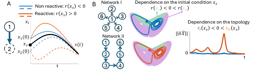
FIG. 1: Schematic summarizing the work of this paper. Panel A illustrates the effects of reactivity on the transient dynamics towards synchronization. Panel B presents two unweighted network topologies one of which (Network II) is more ‘reactive’ than the other one (Network I) and demonstrates the effect of the particular choice of the initial condition and of the network topology on the transient synchronization dynamics. For the example shown, we see the occurrence of jumps in the transverse motion to the synchronization manifold for the more reactive network II (evolution in red), but not for network I (evolution in blue).

We consider networks of diffusively coupled homogeneous oscillators. The network is described by the adjacency matrix $A=[A_{ij}]$, where ${A_{ij}}\geq 0$ measures the strength of the directed coupling from node $j$ to node $i$.The equations that describe the network dynamics are

$$\dot{\pmb{x}}_{i}(t)=\pmb{F}(\pmb{x}_{i}(t))+\sigma\sum_{j=1}^{N}L_{ij}H\pmb{x}_{j}(t),\quad i=1,\ldots,N,$$ (1)

where $\pmb{x}_{i}$ is the $n$-dimensional state of node/oscillator $i$. The individual oscillator dynamics is given by $\pmb{F}(\pmb{x}_{i}(t))$, and the node-to-node coupling interaction is described by the symmetric and positive semidefinite matrix $H$. The more general case that the node-to-node coupling function is nonlinear is studied in Supplementary Note 1. The Laplacian matrix is denoted by $L=[L_{ij}]$ where $L_{ij}=A_{ij}-\delta_{ij}\sum_{j}A_{ij}$, and $\delta_{ij}$ is the Kronecker delta. By construction, $\sum_{j}^{N}L_{ij}=0,\forall i$. The scalar $\sigma\geq 0$ is the coupling strength. We proceed under the assumption (which is required for the stability of the synchronous solution) that the network has a directed spanning tree [51]. Then, the Laplacian matrix has the set of eigenvalues $\{\lambda_{i}\}$, of which $\lambda_{1}=0$ and all the others have negative real parts. Moreover, $\bar{\lambda}_{1}>\bar{\lambda}_{2}\geq...\geq\bar{\lambda}_{N}$, where the bar notation indicates real part.

Equation (1) admits the synchronous solution $\pmb{x}_{1}(t)=\pmb{x}_{2}(t)=...=\pmb{x}_{N}(t)=\pmb{s}(t)$,

$$\dot{\pmb{s}}(t)=\pmb{F}(\pmb{s}(t)),$$ (2)

which is independent of the coupling strength $\sigma$, the Laplacian matrix $L$ and the node-to-node coupling matrix $H$. We call $\mathcal{A}$ the attractor on which the dynamics (2) converges.

The transverse reactivity measures the instantaneous rate of growth or decay of the norm of the state vector of desynchronizing perturbations, and can be thought of as an ‘instantaneous’ finite-time Lyapunov exponent [41]. This relation to finite-time Lyapunov exponents is explained in detail in Supplementary Note 2.

Figure 1 illustrates the concept of transverse reactivity. Panel A shows how the transverse reactivity affects the transient dynamics towards synchronization when synchronization is asymptotically stable. For a given system and set of initial conditions, a non-reactive coupling results in a direct convergence to the synchronous state, while a reactive coupling results in an initial increase in the separation between trajectories before an eventual settling down to the synchronous state in the long term. Panel B presents two unweighted network topologies, one of which is more ‘reactive’ than the other. We consider a network of Lorenz oscillators and color the attractor lavender (green) to indicate points for which the synchronous dynamics are reactive (non-reactive). It is noteworthy that the reactive part of the attractor is larger for the more reactive network than it is for the less reactive one. We compare the time evolutions of the two networks starting from the same initial condition, which has different reactivities for the different network topologies. We plot the distance from the synchronous state $\|\delta\bar{\pmb{X}}(t)\|$ as a function of time. Although both networks eventually achieve synchronization, we see large peaks in the transient time evolution in the case of the more reactive network, while these are not seen in the case of the less-reactive topology. Supplementary Note 3 provides further illustrations of the effects of reactivity on synchronization dynamics by showing how either the choice of the initial conditions or of the network topology affects the occurrence of initial surges in the norm of the motion transverse to the synchronization manifold.

We now provide a precise definition of the transverse reactivity of a point on the attractor. The transverse reactivity of the perturbations about $\pmb{x}_{s}$ on the synchronous solution is given by

$$r(\pmb{x}_{s})=e_{1}\left(\frac{\pmb{D}\pmb{F}({\pmb{x}}_{s})+\pmb{D}\pmb{F}^{\top}({\pmb{x}}_{s})}{2}+\sigma\xi H\right),$$ (3)

where $\pmb{D}\pmb{F}({\pmb{x}}_{s})$ is the Jacobian of $\pmb{F}$ at ${\pmb{x}}_{s}$ and the quantity,

$$\xi=e_{1}\left(V^{\top}\frac{L+{L}^{\top}}{2}V\right)$$ (4)

is often referred to as the algebraic connectivity of directed graphs [51], as a generalization of the classical concept of algebraic connectivity for undirected graphs [52]. The matrix $V\in\mathbb{R}^{N\times N-1}$ is an orthonormal basis for the null subspace of $[1\ 1\ldots 1]\in\mathbb{R}^{1\times N}$, i.e., the matrix $V$ is any matrix with normal columns that are orthogonal to $[1\ 1\ldots 1]^{\top}\in\mathbb{R}^{N}$ and to each other. See Methods V.1 for detailed derivations.

The mapping that associates to each point $\pmb{x}_{s}$ of the attractor $\mathcal{A}$ its transverse reactivity $r(\pmb{x}_{s})$, defines the reactive characterization of the attractor $\mathcal{C}(\mathcal{A})$. A sufficient condition for $\xi=\bar{\lambda}_{2}$ is that the Laplacian matrix $L$ is normal. It also follows that for all undirected networks, $\xi=\lambda_{2}$.

Supplementary Note 4 presents upper and lower bounds for $\xi$. In particular, we prove that $\xi\leq 0$ for minimally reactive networks [39], i.e., a class of networks for which the largest eigenvalue of the symmetric part of the Laplacian is zero. These networks, also known as balanced networks, are such that the in-degree and the out-degrees of each node is the same. Having a negative $\xi$ implies that when the coupling strength is increased, the transverse reactivity of the points on the attractor either decreases or remains constant.

II Efficient Synchronization Dynamics

II.1 Reactivity-based coupling scheme

Our goal is to design a synchronization strategy that is coupling-efficient and energy-efficient; i.e., it requires lower coupling strength on average and lower synchronization energy in comparison to the case of constant coupling. To this end, we find that a simple modification to Eq. (1), in which the constant coupling strength $\sigma$ is replaced by a time varying one $\sigma(t)$, can be extremely beneficial,

$$\dot{\pmb{x}}_{i}(t)=\pmb{F}(\pmb{x}_{i}(t))+\sigma(t)\sum_{j=1}^{N}L_{ij}H\pmb{x}_{j}(t),\quad i=1,\ldots,N.$$ (5)

We call $\pmb{u}_{i}(t)=\sigma(t)\sum_{j=1}^{N}L_{ij}H\pmb{x}_{j}(t)$ the synchronization input affecting node $i$ in Eq. (5) and

$$\mathcal{E}=\dfrac{1}{N}\sum_{i=1}^{N}\dfrac{1}{t_{f}-t_{0}}\int_{t_{0}}^{t_{f}}\|\pmb{u}_{i}(t)\|_{2}dt$$ (6)

the synchronization energy, corresponding to a given choice of the coupling strength $\sigma(t)$ over the time interval $[t_{0},t_{f}]$, where $t_{0}$ and $t_{f}>t_{0}$ are some preassigned times. Here, $\|\cdot\|_{2}$ is the 2-norm.

Our work applies to both cases that the MSF is negative in an unbounded range or bounded range of its argument [2]. When the range is unbounded (often referred to as Class II of the MSF), as we increase $\sigma$ from zero, there is only one transition from asynchrony to synchrony (A $\rightarrow$ S) at the critical value $\sigma^{A\rightarrow S}$. When the range is bounded (Class III of the MSF), as we increase $\sigma$ from zero, first there is a transition from asynchrony to synchrony (A $\rightarrow$ S) at the critical value $\sigma^{A\rightarrow S}$ followed by another transition from synchrony to asynchrony (S $\rightarrow$ A) at the critical value $\sigma^{S\rightarrow A}>\sigma^{A\rightarrow S}$.

First, we consider the case of a transition from asynchrony to synchrony (A $\rightarrow$ S transition), for which the condition for stability of the synchronous solution is that $\sigma>\sigma^{A\rightarrow S}$ (the latter is a function of $\lambda_{2}$). We proceed under the assumption that for a given choice of $\pmb{F}$, $H$, $L$, and constant coupling strength $\bar{\sigma}<\sigma^{A\rightarrow S}$, the coupled oscillators in Eq. (5) will not synchronize. We aim to find a time-varying coupling strength $\sigma(t)$ such that a) the average coupling strength is $1/T\int_{0}^{T}\sigma(t)dt=\bar{\sigma}$, where $T$ is the total time, and b) the coupled dynamical systems in Eq. (5) synchronize. We propose the following simple strategy which we call ‘coupling when needed’ (CWN),

$$\sigma(t)=\begin{cases}\bar{\sigma}\dfrac{1-\gamma(1-\tau)}{\tau},\quad&r(\bar{\pmb{x}}(t))>\beta\\ \\ \bar{\sigma}\gamma,&r(\bar{\pmb{x}}(t))\leq\beta\\ \end{cases}$$ (7)

where $\gamma$ and $\beta$ are tunable parameters such that $0\leq\gamma\leq 1$ and $\beta_{\min}<\beta<\beta_{\max}$. The average solution at time $t$ is $\bar{\pmb{x}}(t)=\frac{1}{N}\sum_{i=1}^{N}\pmb{x}_{i}(t)$, and $\beta_{\min}=\min_{\pmb{x}_{s}\in\mathcal{A}}r(\pmb{x}_{s})$ and $\beta_{\max}=\max_{\pmb{x}_{s}\in\mathcal{A}}r(\pmb{x}_{s})$. The transverse reactivity $r(\bar{\pmb{x}}(t))$ is evaluated at $\bar{\pmb{x}}(t)$ using Eq. (3) with $\sigma=\bar{\sigma}$. Here, the parameter $0<\tau<1$ is the fraction of the times when $r(\bar{\pmb{x}}(t))>\beta$ and is implicitly a function of $\beta$. A good approximation for $\tau$ may be calculated beforehand using a long enough pre-recorded synchronous solution $\pmb{s}(t)$, Eq. (2), as $\tau=1/2+1/2\Big{\langle}\operatorname{sign}\Big{(}r(\pmb{s}(t))-\beta\Big{)}\Big{\rangle}_{t}$. As long as the initial conditions of the connected systems are close to the synchronous solution, the above approximation of $\tau$ is sufficiently close to the actual probability that $r(\bar{\pmb{x}}(t))>\beta$.

If $\gamma=1$, then $\sigma(t)=\bar{\sigma},\ \forall t$, so the time-varying coupling strategy simplifies to the constant coupling. If $\gamma=0$, the CWN strategy becomes on-off, similar to the work of Refs. [53, 8, 54, 55, 56]. A comparison between our work and these references is found in Supplementary Note 5, which shows a strong advantage of our CWN approach.

We now discuss the other case of a transition from synchrony to asynchrony (S $\rightarrow$ A transition), for which the condition for stability of the synchronous solution is that $\sigma<\sigma^{S\rightarrow A}$ (the latter is a function of $\lambda_{N}$). We consider that $\bar{\sigma}$ is greater than the critical coupling $\sigma^{S\rightarrow A}$ predicted by the MSF analysis. Hence, the system of our interest in Eq. (5) will not synchronize if $\sigma(t)=\bar{\sigma}$. Our CWN strategy for the case of an S $\rightarrow$ A transition is,

$$\sigma(t)=\begin{cases}\bar{\sigma}\alpha,\quad&r(\bar{\pmb{x}}(t))>\beta\\ \\ \bar{\sigma}\dfrac{1-\tau\alpha}{1-\tau},&r(\bar{\pmb{x}}(t))\leq\beta\\ \end{cases}$$ (8)

where $0\leq\alpha\leq 1$ and $\beta_{\min}<\beta<\beta_{\max}$ are tunable parameters. See Methods V.2 for detailed derivations of the CWN strategies for both A $\rightarrow$ S and S $\rightarrow$ A transitions.

Supplementary Note 6 shows how this framework can be applied to linear consensus dynamics.

We note here that in the presence of noise or small parametric mismatches, approximate synchronization of the set of Eqs. (1) is still possible, but large desynchronization bursts known as bubbles may occur [57]. While linear stability analysis does not predict these bubbles, we show in Supplementary Note 7 that the transverse reactivity is able to explain them and that they can be eliminated using our coupling scheme.

II.2 Examples

(a) Lorenz                                                      (b) Rössler
       
       

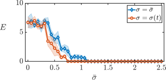
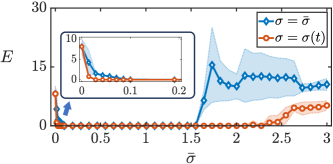
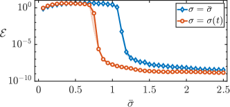
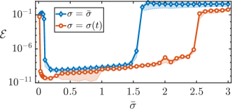
FIG. 2: The synchronization error $E$ (top) and the synchronization energy $\mathcal{E}$ (bottom) versus the average coupling strength $\bar{\sigma}$. Panel (a) shows the case of Lorenz systems. The parameters in Eq. (7) for $\sigma=\sigma(t)$ $\beta=0.5$ and $\gamma=0.16$. Panel (b) shows the case of Rössler oscillators. The parameters for $\sigma=\sigma(t)$ in Eqs. (7) and (8) are $\beta=0.2$ and $\gamma=\alpha=0.01$. For $0\leq\bar{\sigma}<0.3$, we use Eq. (7), and for $0.3\leq\bar{\sigma}\leq 3$, we use Eq. (8). The data for both panels are averaged over 20 realizations initiated from randomly chosen initial conditions. The shaded backgrounds show the standard deviation of the plotted data.

We show the effectiveness of the CWN coupling laws in Eqs. (7) and (8) through examples with coupled Lorenz oscillators and Rössler oscillators. Other examples of different local dynamics such as the Hindmarsh-Rose neuron model, the FitzHugh-Nagumo neuron model, and the forced Van der Pol oscillator are presented in Supplementary Note 8.

We define the synchronization error,

$$E=\left<\frac{1}{N}\sum_{i=1}^{N}\|(\pmb{x}_{i}(t)-\bar{\pmb{x}}(t))\|\right>_{t}.$$ (9)

Here, $<\cdot>_{t}$ returns the average over the time interval $t\in[0.9T\ \ T]$, and we set $T=2000\ s$. The initial conditions for the oscillators are chosen randomly in a small neighborhood of the synchronous solution. For the details of the dynamical function, coupling matrices, and the Laplacian matrix of this example, see Methods V.3.

Figure 2 shows the synchronization error for the oscillators when the coupling strategy in Eq. (5) is

1. constant coupling $\sigma(t)=\bar{\sigma}$

2. time-varying coupling $\sigma(t)$ in either Eqs. (7) or (8).

In the case of an A $\rightarrow$ S transition (S $\rightarrow$ A transition), $\sigma=\sigma(t)$ from Eq. (7) (Eq. (8)) is used. Figure 2 (a) shows the synchronization error $E$ as the average coupling strength $\bar{\sigma}$ is varied for a network of Lorenz oscillators. Here, we set $\gamma=0.16$ and $\beta=0.5$ in Eq. (7). The time-varying coupling strategy $\sigma(t)$ successfully synchronizes the network with $\bar{\sigma}=0.75$ while the constant coupling strategy requires at least $\bar{\sigma}=1.12$. This corresponds to a $33\%$ reduction of the critical average coupling. The lower panel of Fig. 2 (a) also shows that our proposed strategy corresponds to a substantial reduction in energy expenditure compared to the constant coupling strength case. We conclude that our proposed strategy is capable of achieving both i) a reduction in the average coupling strength $\bar{\sigma}$ and ii) a reduction in the synchronization energy $\mathcal{E}$. See Supplementary Note 9 for an in-depth discussion on the energy efficiency of the strategy and how this scales with the average coupling strength $\bar{\sigma}$ for the case of connected Lorenz oscillators.

We now consider the case of Rössler oscillators coupled in the $x$ variable and study separately the two transitions that are seen as the coupling strength is increased: the A $\rightarrow$ S transition followed by the S $\rightarrow$ A transition. In the case of the A $\rightarrow$ S transition, we set $\beta=0.2$ and $\gamma=0.01$ in Eq. (7) and in the case of the S $\rightarrow$ A transition, we set $\beta=0.2$ and $\alpha=0.01$ in Eq. (8). Figure 2 (b) (top) demonstrates a decrease of about 70% of the critical average coupling when the time-varying coupling strategy is implemented for the A $\rightarrow$ S transition and an increase of about 70% of the critical average coupling for the S $\rightarrow$ A transition. Figure 2 (b) (bottom) shows that by the use of time-varying coupling, the synchronization energy $\mathcal{E}$ is also reduced in comparison to constant coupling, which is seen over the entire range of $\bar{\sigma}$ plotted in the figure. We thus conclude that the time-varying coupling strategies in Eq. (7) and (8) can be implemented successfully to significantly expand the range of the coupling strength in which the network synchronizes and to also reduce the synchronization energy $\mathcal{E}$.

We now study the effects of varying the two parameters $\beta$ and $\gamma$ in the synchronization strategy of Eq. (7) for the same system of coupled Lorenz oscillators studied in Fig. 2(a). The local dynamics $\pmb{F}$ and the coupling matrix $H$ are the same as in Eq. (24). The MSF threshold for synchronization is $\sigma^{A\rightarrow S}\bar{\lambda}_{2}\approx-2.3$ as reported in [6]. Here, we wish to see how much smaller we can make $\bar{\sigma}\bar{\lambda}_{2}$ than the MSF threshold and still observe synchronization. To this end, we vary $\gamma$ and $\beta$ in Eq. (7) and find the smallest

$$\text{\% MSF threshold}\ A\rightarrow S=100\dfrac{\sigma^{A\rightarrow S}}{\bar{\sigma}}.$$

Figure 3 shows the % MSF threshold $A\rightarrow S$ as $\gamma$ and $\beta$ are varied for the network with the Laplacian in (26) We see that the switching law in Eq. (7) can successfully synchronize the system for an average value of the coupling as low as 1% of the critical coupling strength corresponding to the MSF threshold.

In Supplementary Note 10, we design a time-varying coupling strategy, similar to the one in Eq. (8), for the case of an S $\rightarrow$ A transition. This strategy is applied to a network of coupled Lorenz oscillators and it is shown that the % MSF threshold for an S $\rightarrow$ A transition can be increased up to five folds (530 %). This significant increase in the upper bound on $\bar{\sigma}$ demonstrates the effectiveness of the time-varying coupling strength in the case of an S $\rightarrow$ A transition.

As a final numerical example, we demonstrate that the synchronization scheme presented in Ref. [50] for the control of extreme events called dragon kings is a special case of our reactivity-based coupling scheme in Supplementary Note 7.

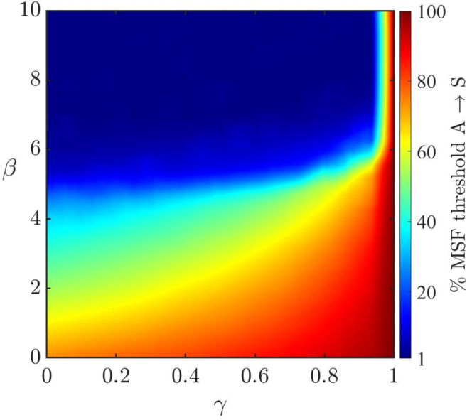
FIG. 3: Effect of the parameter settings on the performance of the control strategy in Eq. (7). % MSF threshold as the parameters $\gamma$ and $\beta$ in Eq. (7) are varied. The Laplacian matrix of the network topology is given in Eq. (26).

II.3 Application to networks of opto-electronic oscillators

We have demonstrated the efficacy of our time-varying coupling scheme in numerical simulations; however, networks in the real world are composed of non-identical oscillators and are subject to noise. Additionally, our coupling scheme relies on a model, which is bound to be imperfect. In this section, we test our reactivity-based coupling scheme on a network of two bi-directionally coupled, chaotic opto-electronic oscillators, and we find that our coupling scheme is robust in an experimental network.

The type of opto-electronic oscillator used here consists of a nonlinear, time-delayed feedback loop. These types of opto-electronic oscillators have found applications in areas such as communications [58], microwave waveform generation [59, 60], and photonic machine learning [61]. A review of these devices can be found in Ref. [62].

A complete description of the opto-electronic oscillator experimental setup and coupling scheme is provided in Supplementary Note 11. A model for the dynamics of our opto-electronic network has been developed in previous work [63]:

$$\begin{split}T\frac{d}{dt}x_{i}(t)=-x(t)+\beta_{fb}\cos^{2}(x_{i}(t-\tau_{D})+\phi_{0})\\ +\sigma(t)\sum_{j=1}^{2}L_{ij}\cos^{2}(x_{j}(t-\tau_{D})+\phi_{0}),\end{split}$$ (10)

where $T$ is the low pass filter characteristic time, $\beta_{fb}$ is the round trip gain, $\sigma$ is the coupling strength, $L$ is the Laplacian coupling matrix, and $\phi_{0}=\pi/4$. In this work, $L_{ij}$ = 1 for $i\neq j$ and $L_{ij}=-1$ for $i=j$. While opto-electronic oscillators can display a wide variety of dynamics [63, 62], we tune our opto-electronic oscillators such that an uncoupled oscillator displays high dimensional chaotic dynamics by selecting $\beta_{fb}=4.0$, $\tau=500\mu s$, and $T=15.9\mu s$.

(a) A $\rightarrow$ S

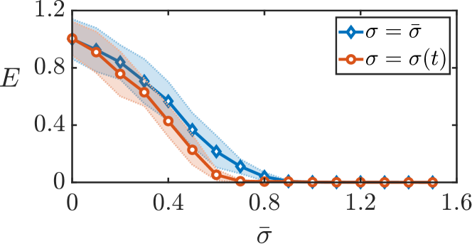
(b) S $\rightarrow$ A

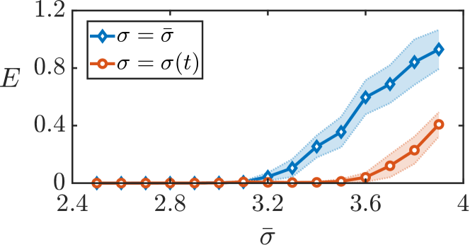
FIG. 4: Demonstration of reactivity-based coupling scheme on experimental network of two coupled opto-electronic oscillators. The synchronization error $E$ is plotted against the average coupling strength $\bar{\sigma}$ for the transitions (a) from asynchrony to synchrony and (b) synchrony to asynchrony. The blue (red) red curves show the constant (time-varying) coupling strategies. The shading shows the standard deviation.

First, to establish a baseline, we keep the coupling strength constant $\sigma=\bar{\sigma}$ and record the voltage applied to the modulator for each oscillator. The synchronization error between the two oscillators is shown in blue in Fig. 4. Next, we implement the time-varying coupling scheme described in Sec. II.1 with $\beta=0.34$, which was determined via numerical simulations of the model Eq. (10). Although Eq. (10) is not in the standard form as Eq. (1), the dynamics of the transverse perturbation is very similar to Eq. (15) (see Supplementary Note 11). The synchronization error with the time-varying coupling scheme is shown in red in Fig. 4. In both cases, the scans over $\bar{\sigma}$ were performed ten times, and the shaded background shows the standard deviation of the measured synchronization errors. One can see that the minimum $\bar{\sigma}$ for A $\rightarrow$ S is reduced from 0.9 to 0.7 and the maximum $\bar{\sigma}$ for S $\rightarrow$ A is increased from 3.2 to 3.5. The results of the energy efficiency are presented in Supplementary Note 11.

We note that the computation of the reactivity relies on the model (Eq. 10) and assumes that the oscillators are identical. These experimental results conclusively demonstrate that the time-varying coupling schemes presented in Sec. II.1 are robust to the imperfect model parameter estimations, non-identical oscillators, and noise that are inherently present in this experiment and in all real-world applications, and that our coupling strategy can be successfully applied to time-delayed systems.

III Network Syncreactivity

An important question is how the particular choice of the network topology affects the reactive characterization of the attractor and what we have discussed so far. We proceed under the assumption that the particular choice of $\pmb{F}$ and $H$ corresponds to a master stability function that is negative in an unbounded range of its argument. The other case in which the range is bounded is discussed in Supplementary Note 12. We now want to compare two different network typologies in terms of the transverse reactivity $r(\pmb{x}_{s})$ and worst-case probability $\mu$. Both these quantities depend on $p=\sigma\xi$. However, for a proper comparison, it is required to pick $\sigma$, such that the long-term stability is the same for both networks. Given two network topologies, with Laplacian matrices $L_{1}$ and $L_{2}$, we fix the coupling strength for each Laplacian matrix such that the long-term stability is the same, that is, $\sigma_{1}\bar{\lambda}_{2}^{1}=\sigma_{2}\bar{\lambda}_{2}^{2}=a<0$, where $\bar{\lambda}_{2}^{1}$ and $\bar{\lambda}_{2}^{2}$ are the real part of the second eigenvalue of the Laplacian matrices $L_{1}$ and $L_{2}$, respectively. Now, we would like to see if $\sigma_{1}\xi_{1}/\sigma_{2}\xi_{2}$ is less, equal, or larger than 1 where $\xi_{1}$ ($\xi_{2}$) is the algebraic connectivity of the Laplacian matrix $L_{1}$ ($L_{2}$), respectively. From Property (ii) for $r(\pmb{x}_{s})$ and the characterization of $\mu$, we know that $r(\pmb{x}_{s})$ and $\mu$ are non-decreasing functions of $\sigma\xi$. Hence, they are higher for the Laplacian matrix $L_{1}$ than for the Laplacian matrix $L_{2}$ if $\sigma_{1}{\xi}_{1}>\sigma_{2}{\xi}_{2}$, or equivalently if the following condition is satisfied, $\xi_{1}/\bar{\lambda}_{2}^{1}<\xi_{2}/\bar{\lambda}_{2}^{2}$. We thus introduce the network syncreactivity index,

$$\Xi=\frac{\xi}{\bar{\lambda_{2}}},$$ (11)

$\Xi\leq 1$ (see Property (i)), and note this is purely a topological measure of the network structureand reflects how reactive that network topology is. If a network is connected and normal, then $\xi=\bar{\lambda}_{2}$ and $\Xi=1$. We emphasize that the network syncreactivity $\Xi$ is a single parameter of the network topology which is responsible for increasing/decreasing the reactive characterization of the attractor $\mathcal{C}(\mathcal{A})$. In particular, if for two networks A and B, $\Xi^{A}<\Xi^{B}$, then $r^{A}(\pmb{x}_{s})\geq r^{B}(\pmb{x}_{s})$ for all $\pmb{x}_{s}\in\mathcal{A}$.

III.1 The syncreactivity of real networks

Since the syncreactivity $\Xi$ is a parameter that solely depends on the structure of a network, it is meaningful to study how this varies among different real networks from available data sets. In what follows, for each network we take the largest strongly connected component (LSCC) and evaluate $\Xi$ for its LSCC. Taking the LSCC of a network ensures that $\bar{\lambda}_{2}\neq 0$ which guarantees synchronizability.

Figure 5 (A) plots the syncreactivity $\Xi$ of networks from different domains versus the network size $N$. We see that on average, neural, trade, biological, and genetics networks are less reactive than social, metabolic, and file-sharing (Gnutella) networks. We also see that most of the more reactive networks have a larger number of nodes. Figure 5 (B) is a plot of the syncreactivity $\Xi$ vs. the density, defined as the number of directed links in the network divided by $N^{2}$, for the same set of real networks in Fig. 5 (A). We see that the density correlates well with the syncreactivity, i.e., sparser (denser) networks have lower (higher) syncreactivity $\Xi$. Figure 5 (C) is a plot of the syncreactivity $\Xi$ vs. the synchronizability index $-\bar{\lambda}_{2}$ (the larger $-\bar{\lambda}_{2}$, the more synchronizable the network) for the same set of real networks in Fig. 5 (A). Networks that are in the top right corner of the plot (e.g., neural) are more synchronizable and less reactive than those in the bottom left corner (e.g., metabolic) and therefore they are more prone to synchronization both transiently and asymptotically. This is consistent with a conjecture that synchronization has been an evolutionary relevant principle in the formation of neural networks, but not in the formation of social, metabolic, and file-sharing networks [64].

In Supplementary Note 13 we have also plotted $\Xi$ vs other measures of synchronizability for directed networks such as the real-part eigenratio $\bar{\lambda}_{2}/\bar{\lambda}_{N}$ and the maximum imaginary part $\mathcal{I}$ among all eigenvalues of the Laplacian [4, 2]. Further information on the real networks considered can be found in the table in Supplementary Note 14.

To conclude, our analysis points out that there are at least two different purely topological indices of the ability of a network to synchronize: the synchronizability, characterizing the asymptotic synchronization dynamics, and the syncreactivity, characterizing the transient synchronization dynamics. We argue here that when comparing different networks topologies in terms of their ability to synchronize, both indices should be taken into account.

(A)

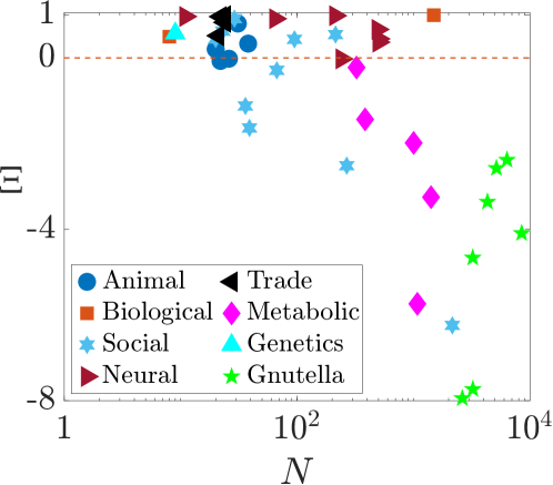
(B)

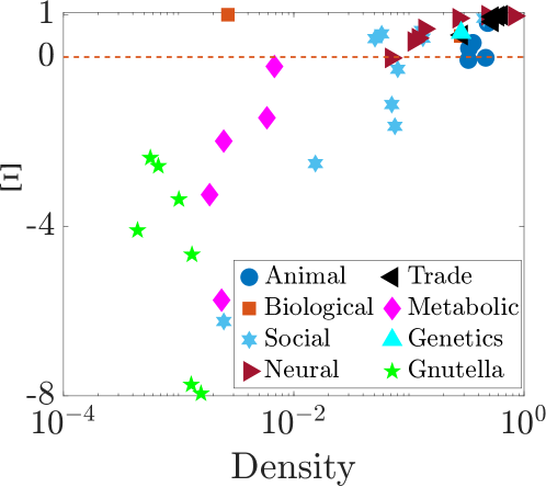
(C)

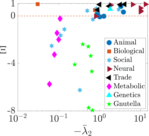
FIG. 5: Real-world examples of complex networks. The syncreactivity $\Xi$ vs (A) the size of the networks $N$, (B) the density, and (C) the negative of the real part of the second Laplacian eigenvalue $-\bar{\lambda}_{2}$ for a collection of real-world networks from different domains.

IV Conclusions

Synchronization is a fundamental physical phenomenon that occurs in networks of coupled technological and biological systems. Much previous work has focused on the asymptotic stability of the synchronous solution, while this paper investigates the transient dynamics and explores the important question of the efficiency of the synchronization dynamics. By combining transient and asymptotic considerations, we achieve an exaustive characterization of the synchronization dynamics of complex networks. This work advances the area of studies on synchronization of networks in more than one direction, as discussed below.

CWN synchronization strategy. All oscillating systems move through regions of phase space that are different from one another: for example, in certain parts of an oscillation, synchronization may be possible for very little coupling or even for no coupling, while other parts may require strong coupling. While the Lyapunov exponents provide average asymptotic measures of stability for a given attractor, they fail at describing transient dynamical behavior. Our work supersedes the Lyapunov exponents analysis by considering a characterization of the reactivity of different regions of the synchronous attractor. This provides the motivation for exploring new synchronization strategies for which the coupling strength is properly adjusted to different parts of oscillations (regions of the synchronous attractor.) Our main result in this paper is the formulation of a synchronization strategy for networks of coupled oscillators that uses coupling only when needed: e.g., for the case that synchronization requires a large enough coupling strength (A $\rightarrow$ S transition), the coupling is increased when the transverse reactivity is large, and it is reduced otherwise. We showed successful application of this strategy in simulations and experiments, and for a variety of different oscillators, including Lorenz, Rössler, the forced Van der Pol, the Hindmarsh-Rose neuron model, the FitzHugh-Nagumo neuron model, and an opto-electronic oscillator experiment, and for different choices of the node-to-node coupling functions. We also showed that CWN provides a rigorous, general foundation for the control of extreme events such as dragon kings, which has previously been thought impossible [50].

Efficiency of the synchronization dynamics. A large part of the literature has focused on the conditions to ensure stability of the synchronized state, while the important issue of the efficiency of the synchronization dynamics has so far received less attention. We investigate the issues of coupling-efficiency and energy-efficiency, which are relevant to both the biological world and technological applications. We propose a synchronization strategy which achieves efficiency by only using coupling when needed. This has immediate benefits in terms of the actuators that can be used to achieve and maintain synchrony. In fact, both technological and biological systems are limited in the duration and overall intensity of the forces that they can exert and benefit from lower energy expenditures. Given the strong advantages we have observed in terms of both average coupling and energy expenditure, it appears likely that coupling and energy-efficient synchronization strategies, similar to the ones we have proposed, may be implemented in the biological world. An example might be that of neuronal short term plasticity, resulting in synaptic enhancement or depression over time scales that are comparable with those of a neuron oscillation.

Enabling Synchronization. Another motivation for this study is the observation that in several practical applications, the type of oscillators, the specific choice of the node-to-node coupling function and of the network topology cannot be changed. Hence, it is meaningful to develop strategies to enable synchronization when it would not occur for a given type of oscillators, network topology, and node-to-node coupling. The MSF approach provides necessary and sufficient conditions for stability of the synchronous state, which makes synchronization outside the intervals predicted by the theory impossible. Here we overcome this limitation by means of a simple synchronization strategy that uses a state dependent coupling strength in place of a constant one. Our proposed synchronization strategy is exceptionally successful at synchronizing networks of coupled oscillators. By using this strategy we were able to show a significant enlargement of the range of the average coupling strength over which synchronization arises. In particular, in the case of an A $\rightarrow$ S transition (S $\rightarrow$ A transition) we could significantly reduce (increase) the critical value of the average coupling strength over which synchronization could be established, sometimes by orders of magnitude. For example, in networks of Lorenz oscillators coupled in the second state variable, we achieved synchrony for an average value of the coupling strength as low as 1% of the critical coupling strength predicted by the MSF analysis.

Network Syncreactivity. We further introduced a new structural network property that characterizes the transient dynamics of networks towards synchronization, which we call network syncreactivity. Several works have linked the reactivity to the non-normality of the dynamics’ Jacobian. It is known that systems characterized by a non-normal Jacobian are prone to transient effects, which may steer their long-term dynamics away from an equilibrium point, even when this is asymptotically stable [65, 34, 66]. For equilibrium points, transient stability can be measured by the reactivity of the fixed point, which is defined as the initial rate of growth of a perturbation about the equilibrium point [30, 38]. We have found that the overall propensity of a network to synchronize can be fully described in terms of two topological scalar indices, synchronizability, and syncreactivity. An analysis of real complex networks from several domains has shown that typically neural networks have better transient and asymptotic synchronization properties than social, metabolic, and file-sharing networks. This is consistent with different evolutionary principles guiding the formation of networks from different domains. We have also identified the density of connections to be a network topological property which well correlates with the syncreactivity, while being distinct from previously introduced topological correlates [34, 38].

Data availability

All data generated or analyzed during this study are included in this published article (and its supplementary information files).

Code availability

The source code for the numerical simulations presented in the paper will be made available upon request.

Author Contributions

Amirhossein Nazerian worked on the theory and numerical simulations. Joe Hart worked on the experimental system, as well as on some aspects of the theory. Matteo Lodi worked on the simulations and the figures. Francesco Sorrentino worked on the theory and supervised the research. All authors contributed to writing the paper.

V Methods

V.1 Isolating the dynamics transverse to the synchronous solution

In order to study the stability of the dynamics of Eqs. (1) about the synchronous solution $\pmb{s}(t)$, we linearized (1) about $\pmb{s}(t)$, thus obtaining,

$$\delta\dot{\pmb{x}}_{i}(t)=\pmb{D}\pmb{F}(\pmb{s}(t))\delta\pmb{x}_{i}(t)+\sigma\sum_{j=1}^{N}L_{ij}H\delta\pmb{x}_{j}(t),$$ (12)

$i=1,...N$, where $\delta\pmb{x}_{i}(t)=\pmb{x}_{i}(t)-\pmb{s}(t)$ is a small perturbation and $\pmb{D}\pmb{F}(\pmb{s}(t))$ is the Jacobian evaluated about the synchronous solution. Equation (12) is rewritten in the compact form as

$$\delta\dot{\pmb{X}}(t)=[I_{N}\otimes\pmb{D}\pmb{F}(\pmb{s}(t))+\sigma L\otimes H]\delta\pmb{X}=Z(t)\delta\pmb{X}(t),$$ (13)

where the $nN$-dimensional vector ${\delta\pmb{X}}^{\top}=[\delta{\pmb{x}}_{1}^{\top},\delta{\pmb{x}}_{2}^{\top},...,\delta{\pmb{x}}_{N}^{\top}]$, $I_{N}$ is the $N$-dimensional identity matrix, and $\otimes$ denotes the Kronecker product. The first challenge, which does not arise in the study of equilibrium points, is that of decoupling the synchronous ‘parallel’ motion from the ‘transverse’ motion.

The variational system (13) has a ‘parallel dynamics’ along the direction spanned by the eigenvector $[\sqrt{N}^{-1},\sqrt{N}^{-1},...,\sqrt{N}^{-1}]^{\top}$ corresponding to the only zero eigenvalue $\lambda_{1}=0$ and a ‘transverse dynamics’ in the subspace orthogonal to this eigenvector. We are especially interested in characterizing the transverse dynamics. In order to isolate this transverse dynamics, we construct an orthogonal matrix $V$ having its first column equal to the vector $[\sqrt{N}^{-1},\sqrt{N}^{-1},\ldots,\sqrt{N}^{-1}]^{\top}$. This can be done, for example, by using the Gram-Schmidt method. Then, we consider the similarity transformation $\tilde{L}=V^{\top}LV$. In the general case in which the matrix $L$ is not symmetric, the matrix $\tilde{L}$ has the following structure,

$$\tilde{L}=\left[\begin{array}[]{@{}c|cccc@{}}0&\tilde{L}_{1,2}&\tilde{L}_{1,3}&\dots&\tilde{L}_{1,N}\\ \hline\cr 0&\tilde{L}_{2,2}&\tilde{L}_{2,3}&\dots&\tilde{L}_{2,N}\\ 0&\vdots&\vdots&\ddots&\vdots\\ 0&\tilde{L}_{N-1,2}&\tilde{L}_{N-1,3}&\dots&\tilde{L}_{N-1,N}\\ 0&\tilde{L}_{N,2}&\tilde{L}_{N,3}&\dots&\tilde{L}_{N,N}\end{array}\right],$$

where we call the $(N-1)$-dimensional block in the right-lower corner the reduced matrix $L^{\perp}$. Alternatively, one can retrieve $L^{\perp}$ by first removing the first column of the matrix $V$ to obtain $\tilde{V}$ and then

$$L^{\perp}=\tilde{V}^{\top}L\tilde{V}.$$ (14)

Note that by construction the matrix $L^{\perp}$ has all negative real-part eigenvalues. Applying the transformation $\tilde{V}$, we can then write down the equation for the time evolutions of the transverse motions corresponding to Eq.(13),

$$\delta\dot{\hat{\pmb{X}}}(t)=[I_{N-1}\otimes\pmb{D}\pmb{F}(\pmb{s}(t))+\sigma L^{\perp}\otimes H]\delta\hat{\pmb{X}}=\hat{Z}(\pmb{s}(t))\delta\hat{\pmb{X}}(t).$$ (15)

We define the transverse reactivity of the perturbations about $\pmb{x}_{s}$ on the synchronous solution

$$\begin{split}r(\pmb{x}_{s}):=&\frac{1}{2}e_{1}\left(\hat{Z}^{\top}(\pmb{x}_{s})+\hat{Z}(\pmb{x}_{s})\right)\\ =&\frac{1}{2}e_{1}\bigg{(}I_{N-1}\otimes[\pmb{D}\pmb{F}({\pmb{x}}_{s})+\pmb{D}\pmb{F}^{\top}({\pmb{x}}_{s})]\\ &\qquad+\sigma({L^{\perp}}^{\top}+L^{\perp})\otimes H\bigg{)}.\end{split}$$ (16)

We remark that the transverse reactivity $r(\pmb{x}_{s})$ determines the reactivity associated with Eq. (15) at a particular point $\pmb{x}_{s}$ on the synchronous solution. If $r(\pmb{x}_{s})>0$ ($r(\pmb{x}_{s})<0$), then the norm of transverse perturbations $\|\delta\hat{\pmb{X}}\|$ can (cannot) increase instantaneously.

We remark that through Eq. (3), the transverse reactivity depends on the parameter $p=\sigma\xi$, where $\sigma\geq 0$ is the coupling strength and $\xi$ is the algebraic connectivity.

Next, we present some properties of the algebraic connectivity $\xi$ and of the transverse reactivity $r(\pmb{x}_{s})$:

1. $\xi\geq\bar{\lambda}_{2}$, i.e., the algebraic connectivity $\xi$ is always greater than or equal to the real part of the second smallest eigenvalue of the Laplacian, $\bar{\lambda}_{2}$.

2. For each point $\pmb{x}_{s}$, the transverse reactivity $r(\pmb{x}_{s})$ (and so the reactive characterization of the attractor) is a continuous monotonically non-decreasing function of the parameter $p=\sigma\xi$.

3. The transverse reactivity $r(\pmb{x}_{s})$ is a continuous function of the synchronous solution $\pmb{s}(t)$ if the Jacobian $\pmb{D}\pmb{F}$ is a continuous function of the synchronous solution.

These properties are proved in the following sections of the Methods. From Property (ii) it follows that the transverse reactivity is a continuous monotonically non-decreasing function of $\xi$ for a fixed $\sigma$. For a fixed $\xi>0$ ($\xi<0$), the transverse reactivity is a continuous monotonically non-decreasing (non-increasing) function of $\sigma$.

Based on Property (iii), we can divide the attractor $\mathcal{A}$ into two distinct regions:

1. The reactive region $\mathcal{R}=\{\pmb{x}_{s}|r(\pmb{x}_{s})>0,\ \pmb{x}_{s}\in\mathcal{A}\}$, and

2. The non-reactive region $\mathcal{N}=\{\pmb{x}_{s}|r(\pmb{x}_{s})\leq 0,\ \pmb{x}_{s}\in\mathcal{A}\}$,

where $\mathcal{R}\bigcap\mathcal{N}=\emptyset$, $\mathcal{R}\bigcup\mathcal{N}=\mathcal{A}$.

We note that for a given choice of the function $\pmb{F}$, the reactivity of these regions is a function of the coupling strength $\sigma$, of the algebraic connectivity $\xi$, and the node-to-node coupling matrix $H$. Thus, if any of the aforementioned parameters change while the local dynamics $\pmb{F}$ is fixed, the reactive and non-reactive regions change too. The ratio between the size of $\mathcal{R}$ and the size of $\mathcal{A}$ defines the critical probability $\mu$ of observing an increase in the norm of the transverse perturbation at the initial time. For detailed information, see Methods Sec. V.7.

In what follows, we will simplify Eq. (16) to obtain Eq. (3). We write down the eigenvalue equation for the symmetric matrix $S_{L^{\perp}}=({L^{\perp}}+{L^{\perp}}^{\top})/2$, $S_{L^{\perp}}V=VY$, where the columns of the orthogonal matrix $V$ are the eigenvectors of the matrix $S_{L^{\perp}}$ and the matrix $Y$ is diagonal with the elements on the main diagonal equal to the eigenvalues of $S_{L^{\perp}}$. We denote the reactivity of $L^{\perp}$, i.e., the largest eigenvalue of its symmetric part, by $\xi=e_{1}\left(S_{L^{\perp}}\right)$. Then, we can rewrite $\mu$ by pre-multiplying and post-multiplying Eq. (16) by $V^{\top}\otimes I$ and $V\otimes I$, respectively, yielding,

$$r(\pmb{x}_{s})=e_{1}(I\otimes[\pmb{D}\pmb{F}({\pmb{x}}_{s})+\pmb{D}\pmb{F}^{\top}({\pmb{x}}_{s})]/2+\sigma Y\otimes H).$$ (17)

Because the matrix $Y$ is diagonal, then

$$r(\pmb{x}_{s})=\max_{i}\Bigl{\{}e_{1}([\pmb{D}\pmb{F}({\pmb{x}}_{s})+\pmb{D}\pmb{F}^{\top}({\pmb{x}}_{s})]/2+\sigma Y_{ii}H)\Bigr{\}}.$$ (18)

From Eq. (18), we also see that there are two distinct effects on the overall transverse reactivity, a baseline effect of the individual dynamics given by $[\pmb{D}\pmb{F}({\pmb{x}}_{s})+\pmb{D}\pmb{F}^{\top}({\pmb{x}}_{s})]/2$ and an effect of the network topology given by $Y_{ii}$. The baseline effect depends on the particular choice of the function $\pmb{F}$ so that different choices of oscillators result in different baseline effects. In what follows we are particularly interested in the role of the network topology and so focus on the largest eigenvalue of $S_{L^{\perp}}$. By the assumption that $H$ is positive semidefinite, application of Weyl’s inequalities [67] yields,

$$\begin{split}e_{1}([\pmb{D}\pmb{F}({\pmb{x}}_{s})+&\pmb{D}\pmb{F}^{\top}({\pmb{x}}_{s})]/2+\sigma Y_{ii}H)\\ &\leq e_{1}([\pmb{D}\pmb{F}({\pmb{x}}_{s})+\pmb{D}\pmb{F}^{\top}({\pmb{x}}_{s})]/2)\end{split}$$

Also, under the generic assumption that the matrices have simple spectra one can show that (see [68, Chapter 1.3.4])

$$\frac{de_{1}([\pmb{D}\pmb{F}({\pmb{x}}_{s})+\pmb{D}\pmb{F}^{\top}({\pmb{x}}_{s})]/2+\sigma Y_{ii}H)}{dY_{ii}}={\pmb{\pi}}^{\top}\sigma H{\pmb{\pi}}\geq 0,$$

where ${\pmb{\pi}}$ is the Perron-Frobenius eigenvector (with entries all of the same sign) of the symmetric matrix $[\pmb{D}\pmb{F}({\pmb{x}}_{s})+\pmb{D}\pmb{F}^{\top}({\pmb{x}}_{s})]/2+\sigma Y_{ii}H$. We thus expect the maximum in Eq. (18) to be always achieved for $i=i^{*}$ corresponding to the reactivity of $L^{\perp}$, i.e., $\xi$. Then, Eq. (16) for the reactivity of the transverse motion is rewritten as

$$r(\pmb{x}_{s})=e_{1}\left(\frac{\pmb{D}\pmb{F}({\pmb{x}}_{s})+\pmb{D}\pmb{F}^{\top}({\pmb{x}}_{s})}{2}+\sigma\xi H\right),$$

which is the same as Eq. (3).

V.2 Coupling when needed

We aim to find a time-varying coupling strength $\sigma(t)$ such that a) the average coupling strength is

$$\frac{1}{T}\int_{0}^{T}\sigma(t)dt=\bar{\sigma},$$ (19)

where $T$ is the total time, and b) the coupled dynamical systems in Eq. (5) synchronize. We propose the following simple strategy which we call ‘coupling when needed’ (CWN),

$$\sigma(t)=\begin{cases}\sigma_{1},\quad&r(\bar{\pmb{x}}(t))>\beta\\ \sigma_{2},&r(\bar{\pmb{x}}(t))\leq\beta\\ \end{cases}$$ (20)

where $\bar{\pmb{x}}(t)=\frac{1}{N}\sum_{i=1}^{N}\pmb{x}_{i}(t)$ is the average solution at time $t$, $\beta_{\min}<\beta<\beta_{\max}$ is a tunable parameter, between $\beta_{\min}=\min_{\pmb{x}_{s}\in\mathcal{A}}r(\pmb{x}_{s})$ and $\beta_{\max}=\max_{\pmb{x}_{s}\in\mathcal{A}}r(\pmb{x}_{s})$, and

$$r(\bar{\pmb{x}}(t))=e_{1}\left(\frac{\pmb{D}\pmb{F}(\bar{\pmb{x}}(t))+\pmb{D}\pmb{F}^{\top}(\bar{\pmb{x}}(t))}{2}+\bar{\sigma}\xi H\right).$$ (21)

Here, $\xi$ is the previously introduced algebraic connectivity of the Laplacian $L$. We proceed to find $\sigma_{1}$ and $\sigma_{2}$ such that $\sigma_{1}\geq\bar{\sigma}\geq\sigma_{2}>0$ and Eq. (19) is satisfied.

Without loss of generality, we can set $\sigma_{1}=\bar{\sigma}/\alpha$ and $\sigma_{2}=\bar{\sigma}\gamma$ where $0<\alpha\leq 1$ and $0\leq\gamma\leq 1$. By enforcing the constraint in Eq. (19), we get

$$\frac{1}{T}\int_{0}^{T}\sigma(t)dt\approx\frac{1}{T}\left(\tau T\frac{\bar{\sigma}}{\alpha}+(1-\tau)T\bar{\sigma}\gamma\right)=\bar{\sigma}.$$

Here, the parameter $0<\tau<1$ is the fraction of the times when $r(\bar{\pmb{x}}(t))>\beta$ and is implicitly a function of $\beta$. After simplifications, we obtain $1/\alpha=(1-\gamma(1-\tau))/\tau$. Thus, Eq. (20) is rewritten as

$$\sigma(t)=\begin{cases}\bar{\sigma}\dfrac{1-\gamma(1-\tau)}{\tau},\quad&r(\bar{\pmb{x}}(t))>\beta\\ \\ \bar{\sigma}\gamma,&r(\bar{\pmb{x}}(t))\leq\beta\\ \end{cases}$$ (22)

where $\gamma$ and $\beta$ are tunable parameters such that $0\leq\gamma\leq 1$ and $\beta_{\min}<\beta<\beta_{\max}$. If $\gamma=1$, then $\sigma(t)=\bar{\sigma},\ \forall t$, so the time-varying coupling strategy simplifies to the constant coupling. If $\gamma=0$ our strategy becomes on-off, similar to the work of Refs. [53, 8, 54, 55, 56]. A comparison between our work and these references is found in Supplementary Note 5, which shows the superiority of our CWN approach. A good approximation for $\tau$ may be calculated beforehand using a long enough pre-recorded synchronous solution $\pmb{s}(t)$, Eq. (2), as

$$\tau=\frac{1}{2}+\frac{1}{2}\Big{\langle}\operatorname{sign}\Big{(}r(\pmb{s}(t))-\beta\Big{)}\Big{\rangle}_{t}.$$

As long as the initial conditions of the connected systems are close to the synchronous solution, the above approximation of $\tau$ is sufficiently close to the actual probability that $r(\bar{\pmb{x}}(t))>\beta$.

We now focus on the other case of a transition from synchrony to asynchrony (S $\rightarrow$ A transition), for which the condition for stability of the synchronous solution is that $\sigma<\sigma^{S\rightarrow A}$ (the latter is a function of $\lambda_{N}$). We consider that $\bar{\sigma}$ is greater than the critical coupling $\sigma^{S\rightarrow A}$ predicted by the MSF analysis. Hence, the system of our interest in Eq. (5) will not synchronize if $\sigma(t)=\bar{\sigma}$.

To synchronize the system under a state-dependent coupling strategy with an average value of $\bar{\sigma}$, we use the same coupling strategy in Eq. (20) but for this case, we set $0<\sigma_{1}\leq\bar{\sigma}\leq\sigma_{2}$. Without loss of generality, we can take $\sigma_{1}=\bar{\sigma}\alpha$ and $\sigma_{2}=\bar{\sigma}/\gamma$ where $0<\alpha\leq 1$ and $0<\gamma\leq 1$ are tunable parameters. After enforcing the constraint in Eq. (19), we obtain $1/\gamma=(1-\tau\alpha)/(1-\tau)$, where $\tau$ is the fraction of the times when $r(\bar{\pmb{x}}(t))>\beta$, as before. Therefore, our CWN strategy for the case of an S $\rightarrow$ A transition is,

$$\sigma(t)=\begin{cases}\bar{\sigma}\alpha,\quad&r(\bar{\pmb{x}}(t))>\beta\\ \\ \bar{\sigma}\dfrac{1-\tau\alpha}{1-\tau},&r(\bar{\pmb{x}}(t))\leq\beta\\ \end{cases}$$ (23)

where $0\leq\alpha\leq 1$ and $\beta_{\min}<\beta<\beta_{\max}$ are tunable parameters.

V.3 Example details

The local dynamics $\pmb{F}$ and the coupling matrix $H$ for the case of Lorenz are

$$\pmb{x}=\begin{bmatrix}x\\ y\\ z\end{bmatrix},\ \ \pmb{F}(\pmb{x})=\begin{bmatrix}10(y-x)\\ x(28-z)-y\\ xy-2z\end{bmatrix},\ \ H=\begin{bmatrix}0&0&0\\ 0&1&0\\ 0&0&0\end{bmatrix},$$ (24)

which results in an unbounded range of the coupling strength for synchronization. For the case of the Rössler oscillator, we set

$$\pmb{x}=\begin{bmatrix}x\\ y\\ z\end{bmatrix},\ \ \pmb{F}(\pmb{x})=\begin{bmatrix}-y-x\\ x+0.2y\\ 0.2+(x-9)z\end{bmatrix},\ \ H=\begin{bmatrix}1&0&0\\ 0&0&0\\ 0&0&0\end{bmatrix},$$ (25)

which results in a bounded range of the coupling strength that produces synchronization. We randomly construct a directed unweighted graph, with Laplacian

$$L=\begin{bmatrix}-1&0&1&0\\ 1&-2&1&0\\ 0&1&-1&0\\ 1&1&1&-3\end{bmatrix}.$$ (26)

V.4 Proof of Property (i)

Property (i) follows from the fact that the largest eigenvalue of the symmetric part of a matrix is always greater than or equal to the largest real part eigenvalue of that matrix; therefore $\xi\geq\bar{\lambda}_{2}$. The inequality is satisfied with the equal sign, i.e., $\xi=\bar{\lambda}_{2}$, whenever the left and the right eigenvectors of $L^{\perp}$ are real and coincide. The proof is complete. ∎

V.5 Proof of Property (ii)

We fix a point on the synchronous solution, $\pmb{x}_{s}\in\{\pmb{s}(t)\}$. Then, for an assigned Jacobian $\pmb{D}\pmb{F}(\pmb{x}_{s})$ and coupling matrix $H$, we look at the effects of varying $\sigma\xi$ on the eigenvalues of the matrix

$$M=\frac{\pmb{D}\pmb{F}({\pmb{x}}_{s})+\pmb{D}\pmb{F}^{\top}({\pmb{x}}_{s})}{2}+\sigma\xi H.$$

As $\sigma\xi$ changes continuously, the entries of the matrix $M$ vary continuously as well. It is well known that the eigenvalues of a matrix vary continuously with the entries of the matrix. Therefore, $r(\pmb{x}_{s})$ varies continuously with $\sigma\xi$. Also, under the generic assumption that the matrices have simple spectra, one can show that (see [68, Chapter 1.3.4])

$$\frac{d(r(\pmb{x}_{s}))}{d(\sigma\xi)}=\frac{de_{1}(M)}{d(\sigma\xi)}={\pmb{\pi}}^{\top}H{\pmb{\pi}}\geq 0,$$

where ${\pmb{\pi}}$ is the Perron-Frobenius eigenvector (with entries all of the same sign) of the symmetric matrix $M$. Hence, $r(\pmb{x}_{s})$ is a continuous monotonically non-decreasing function of $\sigma\xi$. The proof is complete. ∎

V.6 Proof of Property (iii)

Consider the matrix

$$M=\frac{\pmb{D}\pmb{F}({\pmb{x}}_{s})+\pmb{D}\pmb{F}^{\top}({\pmb{x}}_{s})}{2}+\sigma\xi H$$

for a point on the attractor, $\pmb{x}_{s}\in\mathcal{A}$. If we assume that $\pmb{D}\pmb{F}({\pmb{x}}_{s})$ is a continuous function of ${\pmb{x}}_{s}$, it follows the entries of $M$ are a continuous function of $\pmb{x}_{s}$. Also, it is known that the eigenvalues of a matrix are continuous functions of the entries of that matrix. Thus, we conclude the transverse reactivity $r(\pmb{x}_{s})=e_{1}(M)$ is a continuous function of $\pmb{x}_{s}$. The proof is complete. ∎

V.7 Worst-case probability

Here we define the ‘worst-case’ probability of observing an increase in the norm of the transverse perturbation at initial times by randomly selecting a point $\pmb{x}_{s}$ from the attractor:

$$\mu:=\frac{1}{2}+\frac{1}{2}\Big{\langle}\operatorname{sign}\Big{(}r(\pmb{x}_{s})\Big{)}\Big{\rangle}_{\mathcal{A}}.$$ (27)

Here, $\operatorname{sign}(\cdot)$ is the sign function and $<\cdot>_{\mathcal{A}}$ indicates an average over the attractor $\mathcal{A}$. The quantity $0\leq\mu\leq 1$ measures the fraction of the points on the attractor that result in $r(\pmb{x}_{s})>0$ for some values of $\sigma$ and $\xi$. The term ‘worst-case’ refers to the worst possible choice of the initial condition $\delta\hat{\pmb{X}}(0)$ for Eq. (15), which is a scalar multiple of the eigenvector corresponding to the largest eigenvalue of the matrix $(\hat{Z}(\pmb{x}_{s})+\hat{Z}(\pmb{x}_{s})^{\top})/2$. However, if $\delta\hat{\pmb{X}}(0)$ is chosen randomly, the initial condition will have a nonzero component along this eigenvector with probability one. Hence, by defining $\mu$ as above, we now can provide a probability that an increase in $\|\delta\hat{\pmb{X}}(t)\|$ will be typically seen at the initial time.

Proposition 1.

The worst-case probability $\mu$ is a monotonically non-decreasing function of $p$.

Proof.

Since $\mu$ is a non-decreasing continuous function of $r(\pmb{x}_{s})$ and $r(\pmb{x}_{s})$ is a non-decreasing continuous function of $p=\sigma\xi$, we conclude $\mu$ is a non-decreasing continuous function of $p$. The proof is complete. ∎

References

- [1] Strogatz, S. Sync: The Emerging Science of Spontaneous Order (Hyperion. New York, 2003).
- [2] Boccaletti, S., Latora, V., Moreno, Y., Chavez, M. & Hwang, D. U. Complex networks: Structure and dynamics. Phys. Rep. 424, 175–308 (2006).
- [3] Pecora, L. & Carroll, T. Master stability functions for synchronized coupled systems. Phys. Rev. Lett. 80, 2109–2112 (1998).
- [4] Barahona, M. & Pecora, L. Synchronization in small-world networks. Phys. Rev. Lett. 89, 054101 (2002).
- [5] Pikovsky, A., Rosenblum, M. & Kurths, J. Synchronization: a universal concept in nonlinear science (2002).
- [6] Huang, L., Chen, Q., Lai, Y.-C. & Pecora, L. M. Generic behavior of master-stability functions in coupled nonlinear dynamical systems. Phys. Rev. E 80, 036204 (2009).
- [7] Schiff, S. J., So, P., Chang, T., Burke, R. E. & Sauer, T. Detecting dynamical interdependence and generalized synchrony through mutual prediction in a neural ensemble. Physical Review E 54, 6708 (1996).
- [8] So, P., Cotton, B. C. & Barreto, E. Synchronization in interacting populations of heterogeneous oscillators with time-varying coupling. Chaos: An Interdisciplinary Journal of Nonlinear Science 18 (2008).
- [9] Carletti, T., Serra, R., Poli, I., Villani, M. & Filisetti, A. Sufficient conditions for emergent synchronization in protocell models. Journal of theoretical biology 254, 741–751 (2008).
- [10] Toiya, M., González-Ochoa, H. O., Vanag, V. K., Fraden, S. & Epstein, I. R. Synchronization of chemical micro-oscillators. The Journal of Physical Chemistry Letters 1, 1241–1246 (2010).
- [11] Stout, J., Whiteway, M., Ott, E., Girvan, M. & Antonsen, T. M. Local synchronization in complex networks of coupled oscillators. Chaos: An Interdisciplinary Journal of Nonlinear Science 21 (2011).
- [12] Latora, V. et al. Stability of synchronization in simplicial complexes. Nature Communications (2021).
- [13] Nazerian, A. et al. Matryoshka and disjoint cluster synchronization of networks. Chaos: An Interdisciplinary Journal of Nonlinear Science 32 (2022).
- [14] Bhatta, K., Nazerian, A. & Sorrentino, F. Supermodal decomposition of the linear swing equation for multilayer networks. IEEE Access 10, 72658–72670 (2022).
- [15] Nazerian, A., Panahi, S. & Sorrentino, F. Synchronization in networks of coupled oscillators with mismatches. Europhysics Letters 143, 11001 (2023).
- [16] Nazerian, A., Nathe, C., Hart, J. D. & Sorrentino, F. Synchronizing chaos using reservoir computing. Chaos: An Interdisciplinary Journal of Nonlinear Science 33, 103121 (2023).
- [17] Nazerian, A., Panahi, S. & Sorrentino, F. Synchronization in networked systems with large parameter heterogeneity. Communications Physics 6, 253 (2023).
- [18] Locatelli, N. et al. Efficient synchronization of dipolarly coupled vortex-based spin transfer nano-oscillators. Scientific reports 5, 17039 (2015).
- [19] Moujahid, A., d’Anjou, A., Torrealdea, F. & Torrealdea, F. Efficient synchronization of structurally adaptive coupled hindmarsh–rose neurons. Chaos, Solitons & Fractals 44, 929–933 (2011).
- [20] Zhang, D., Cao, Y., Ouyang, Q. & Tu, Y. The energy cost and optimal design for synchronization of coupled molecular oscillators. Nature physics 16, 95–100 (2020).
- [21] Urazhdin, S., Tabor, P., Tiberkevich, V. & Slavin, A. Fractional synchronization of spin-torque nano-oscillators. Physical review letters 105, 104101 (2010).
- [22] Murali, K. & Lakshmanan, M. Transmission of signals by synchronization in a chaotic van der pol–duffing oscillator. Physical Review E 48, R1624 (1993).
- [23] Demidov, V. et al. Synchronization of spin hall nano-oscillators to external microwave signals. Nature communications 5, 3179 (2014).
- [24] Izhikevich, E. M. Dynamical systems in neuroscience (MIT press, 2007).
- [25] McCrea, M., Ermentrout, B. & Rubin, J. E. A model for the collective synchronization of flashing in photinus carolinus. Journal of the Royal Society Interface 19, 20220439 (2022).
- [26] Ramírez-Ávila, G. M., Kurths, J., Depickere, S. & Deneubourg, J.-L. Modeling fireflies synchronization. A mathematical modeling approach from nonlinear dynamics to complex systems 131–156 (2019).
- [27] Verkerk, A. O. et al. Single cells isolated from human sinoatrial node: action potentials and numerical reconstruction of pacemaker current. In 2007 29th Annual international conference of the IEEE Engineering in Medicine and Biology Society, 904–907 (IEEE, 2007).
- [28] Dokos, S., Celler, B. & Lovell, N. Ion currents underlying sinoatrial node pacemaker activity: a new single cell mathematical model. Journal of theoretical biology 181, 245–272 (1996).
- [29] Farrell, B. F. & Ioannou, P. J. Generalized stability theory. part i: Autonomous operators. Journal of Atmospheric Sciences 53, 2025 – 2040 (1996).
- [30] Neubert, M. G. & Caswell, H. Alternatives to resilience for measuring the responses of ecological systems to perturbations. Ecology 78, 653–665 (1997).
- [31] Hennequin, G., Vogels, T. P. & Gerstner, W. Non-normal amplification in random balanced neuronal networks. Phys. Rev. E 86, 011909 (2012).
- [32] Tang, S. & Allesina, S. Reactivity and stability of large ecosystems. Frontiers in Ecology and Evolution 2 (2014).
- [33] Biancalani, T., Jafarpour, F. & Goldenfeld, N. Giant amplification of noise in fluctuation-induced pattern formation. Phys. Rev. Lett. 118, 018101 (2017).
- [34] Asllani, M., Lambiotte, R. & Carletti, T. Structure and dynamical behavior of non-normal networks. Science advances 4, eaau9403 (2018).
- [35] Muolo, R., Asllani, M., Fanelli, D., Maini, P. K. & Carletti, T. Patterns of non-normality in networked systems. Journal of Theoretical Biology 480, 81–91 (2019).
- [36] Gudowska-Nowak, E., Nowak, M. A., Chialvo, D. R., Ochab, J. K. & Tarnowski, W. From Synaptic Interactions to Collective Dynamics in Random Neuronal Networks Models: Critical Role of Eigenvectors and Transient Behavior. Neural Computation 32, 395–423 (2020).
- [37] Lindmark, G. & Altafini, C. Centrality measures and the role of non-normality for network control energy reduction. IEEE Control Systems Letters 5, 1013–1018 (2021).
- [38] Duan, C., Nishikawa, T., Eroglu, D. & Motter, A. E. Network structural origin of instabilities in large complex systems. Science advances 8, eabm8310 (2022).
- [39] Nazerian, A., Phillips, D., Makse, H. A. & Sorrentino, F. Single-integrator consensus dynamics over minimally reactive networks. IEEE Control Systems Letters (2023).
- [40] Nazerian, A., Phillips, D., Frasca, M. & Sorrentino, F. The reactability of discrete time systems. IEEE Control Systems Letters 7, 3657–3662 (2023).
- [41] Pikovsky, A. & Politi, A. Lyapunov exponents: a tool to explore complex dynamics (Cambridge University Press, 2016).
- [42] Olfati-Saber, R. & Murray, R. Consensus problems in networks of agents with switching topology and time-delays. IEEE Transactions on Automatic Control 49, 1520–1533 (2004).
- [43] Olfati-Saber, R., Fax, A. & Murray, R. M. Consensus and cooperation in networked multi-agent systems. Proceedings of the IEEE 95, 215–233 (2007).
- [44] Miao, Z., Wang, Y. & Fierro, R. Collision-free consensus in multi-agent networks: A monotone systems perspective. Automatica 64, 217–225 (2016).
- [45] Liu, X., Chen, T. & Lu, W. Consensus problem in directed networks of multi-agents via nonlinear protocols. Physics Letters A 373, 3122–3127 (2009).
- [46] Liu, Y.-Y., Slotine, J.-J. & Barabási, A.-L. Controllability of complex networks. nature 473, 167–173 (2011).
- [47] Yan, G. et al. Spectrum of controlling and observing complex networks. Nature Physics (2015).
- [48] Sorrentino, F., di Bernardo, M., Garofalo, F. & Chen, G. Controllability of complex networks via pinning. Phys. Rev. E 75, 046103 (2007).
- [49] Panahi, S., Lodi, M., Storace, M. & Sorrentino, F. Pinning control of networks: Dimensionality reduction through simultaneous block-diagonalization of matrices. Chaos: An Interdisciplinary Journal of Nonlinear Science 32 (2022).
- [50] de S. Cavalcante, H. L. D., Oriá, M., Sornette, D., Ott, E. & Gauthier, D. J. Predictability and suppression of extreme events in a chaotic system. Phys. Rev. Lett. 111, 198701 (2013).
- [51] Wu, C. W. Algebraic connectivity of directed graphs. Linear and multilinear algebra 53, 203–223 (2005).
- [52] Fiedler, M. Algebraic connectivity of graphs. Czechoslovak mathematical journal 23, 298–305 (1973).
- [53] Belykh, I. V., Belykh, V. N. & Hasler, M. Blinking model and synchronization in small-world networks with a time-varying coupling. Physica D: Nonlinear Phenomena 195, 188–206 (2004).
- [54] Chen, F., Chen, Z., Xiang, L., Liu, Z. & Yuan, Z. Reaching a consensus via pinning control. Automatica 45, 1215–1220 (2009).
- [55] Buscarino, A., Frasca, M., Branciforte, M., Fortuna, L. & Sprott, J. C. Synchronization of two rössler systems with switching coupling. Nonlinear Dynamics 88, 673–683 (2017).
- [56] Parastesh, F. et al. Synchronizability of two neurons with switching in the coupling. Applied Mathematics and Computation 350, 217–223 (2019).
- [57] Ashwin, P., Buescu, J. & Stewart, I. Bubbling of attractors and synchronisation of chaotic oscillators. Physics Letters A 193, 126–139 (1994).
- [58] Argyris, A. et al. Chaos-based communications at high bit rates using commercial fibre-optic links. Nature 438, 343–346 (2005).
- [59] Maleki, L. The optoelectronic oscillator. Nat. Photon. 5, 728–730 (2011).
- [60] Hao, T. et al. Breaking the limitation of mode building time in an optoelectronic oscillator. Nat. Commun. 9, 1839 (2018).
- [61] Larger, L. et al. Photonic information processing beyond turing: an optoelectronic implementation of reservoir computing. Opt. Express 20, 3241–3249 (2012).
- [62] Chembo, Y. K., Brunner, D., Jacquot, M. & Larger, L. Optoelectronic oscillators with time-delayed feedback. Rev. Mod. Phys. 91, 035006 (2019).
- [63] Murphy, T. E. et al. Complex dynamics and synchronization of delayed-feedback nonlinear oscillators. Phil. Trans. R. Soc. A 368, 343–366 (2010).
- [64] Montgomery, R. & Md, M. Evolutionary origins and functional diversity of neural synchronization and desynchronization: A multidisciplinary perspective. ResearchGate preprint RG.2.2.12019.71203 (2023).
- [65] Trefethen, L. N., Trefethen, A. E., Reddy, S. C. & Driscoll, T. A. Hydrodynamic stability without eigenvalues. Science 261, 578–584 (1993).
- [66] Asllani, M. & Carletti, T. Topological resilience in non-normal networked systems. Physical Review E 97, 042302 (2018).
- [67] Horn, R. A., Rhee, N. H. & Wasin, S. Eigenvalue inequalities and equalities. Linear Algebra and its Applications 270, 29–44 (1998).
- [68] Tao, T. Topics in random matrix theory, vol. 132 (American Mathematical Soc., 2012).