Universität Würzburg, Germany firstname +++ dot +++ lastname +++ at +++ uni +++ minus +++ wuerzburg +++ dot +++ dehttps://orcid.org/0000-0002-4532-3765Universität Würzburg, Germanymarie.sieper@uni-wuerzburg.dehttps://orcid.org/0009-0003-7491-2811 \CopyrightBoris Klemz and Marie Diana Sieper \ccsdesc[500]Theory of computation Fixed parameter tractability \ccsdesc[500]Human-centered computing Graph drawings \ccsdesc[300]Mathematics of computing Graphs and surfaces \ccsdesc[100]Theory of computation Computational geometry \ccsdesc[100]Mathematics of computing Paths and connectivity problems \EventEditorsJohn Q. Open and Joan R. Access \EventNoEds2 \EventLongTitle42nd Conference on Very Important Topics (CVIT 2016) \EventShortTitleCVIT 2016 \EventAcronymCVIT \EventYear2016 \EventDateDecember 24–27, 2016 \EventLocationLittle Whinging, United Kingdom \EventLogo \SeriesVolume42 \ArticleNo23
Constrained Level Planarity is FPT with Respect to the Vertex Cover Number
Abstract
The problem Level Planarity asks for a crossing-free drawing of a graph in the plane such that vertices are placed at prescribed y-coordinates (called levels) and such that every edge is realized as a y-monotone curve. In the variant Constrained Level Planarity, each level is equipped with a partial order on its vertices and in the desired drawing the left-to-right order of vertices on level has to be a linear extension of . Constrained Level Planarity is known to be a remarkably difficult problem: previous results by Klemz and Rote [ACM Trans. Alg.’19] and by Brückner and Rutter [SODA’17] imply that it remains NP-hard even when restricted to graphs whose tree-depth and feedback vertex set number are bounded by a constant and even when the instances are additionally required to be either proper, meaning that each edge spans two consecutive levels, or ordered, meaning that all given partial orders are total orders. In particular, these results rule out the existence of FPT-time (even XP-time) algorithms with respect to these and related graph parameters (unless P=NP). However, the parameterized complexity of Constrained Level Planarity with respect to the vertex cover number of the input graph remained open.
In this paper, we show that Constrained Level Planarity can be solved in FPT-time when parameterized by the vertex cover number. In view of the previous intractability statements, our result is best-possible in several regards: a speed-up to polynomial time or a generalization to the aforementioned smaller graph parameters is not possible, even if restricting to proper or ordered instances.
keywords:
Parameterized Complexity, Graph Drawing, Planar Poset Diagram, Level Planarity, Constrained Level Planarity, Vertex Cover, FPT, Computational Geometry1 Introduction
A large body of literature related to graph drawing is dedicated to so-called upward planar drawings, which provide a natural way of visualizing a partial order on a set of items. An upward planar drawing of a directed graph is a crossing-free drawing in the plane where every edge is realized as a y-monotone curve that goes upwards from to , i.e., the y-coordinate strictly increases when traversing from towards . The most classical computational problem in this context is Upward Planarity: given a directed graph, decide whether it admits an upward planar drawing. The standard version of this problem is NP-hard [18], but, if the y-coordinate of each vertex is prescribed, it can be solved in polynomial time [13, 21, 25], which suggests that a large part of the challenge of Upward Planarity comes from choosing an appropriate y-coordinate for each vertex. However, when both the y-coordinate and the x-coordinate of each vertex are prescribed, the problem is yet again NP-hard [27], indicating that another part of the challenge comes from drawing the edges in a y-monotone non-crossing fashion while respecting the given or chosen coordinates of their endpoints. The paper at hand is concerned with the parameterized complexity of a generalization of the latter of these two variants of Upward Planarity, which is known as Constrained Level Planarity. It is expressed in terms of so-called level graphs, which are defined next; we adopt the notation and terminology used in [27].
Level Planarity.
A level graph is a directed graph together with a level assignment, which is a function111 Traditionally, in the literature, the level assignment is defined as a surjective function that maps to an integer interval ; it merely acts as a convenient way to encode a total preorder on . It is well known that the traditional and our (more general) definition are polynomial-time equivalent: algorithms designed assuming the classical definition can also be applied in the more general context: one simple has to first sort the vertices by y-coordinates and then apply the traditional algorithm using the sorting-ranks as y-coordinates. We are using the given general definition as it eases the description of our algorithms; though, specific polynomial runtimes obtained in previous work that are stated in our introduction assume the classical definition. where for every edge . For every where is non-empty, the set is called a (the -th) level of . The width of level is . The level-width of is the maximum width of any level in and the height of is the number of (non-empty) levels. A level planar drawing of is an upward planar drawing of where the y-coordinate of each vertex is . We use to denote the horizontal line with y-coordinate . The level graph is called proper if every edge spans two consecutive levels, that is, for every edge there is no level with . The problem Level Planarity asks whether a given level graph admits a level planar drawing. In a series of papers [13, 21, 24, 25], it was shown that Level Planarity can be solved in linearFootnote 1 time; we refer to [16] for a more detailed discussion of the history of the corresponding algorithm and of alternative approaches to solve Level Planarity.
Constrained Level Planarity.
In 2017, Brückner and Rutter [8] and Klemz and Rote [27] independently introduced and studied two closely related variants of Level Planarity, which are defined in the following. A constrained level graph is a triple corresponding to a level graph equipped with a family containing, for each level , a partial order on the vertices . A constrained level planar drawing of is a level planar drawing of where, for each level , the left-to-right order of the vertices corresponds to a linear extension of . For a pair of vertices with , we refer to as a constraint on and . The problem Constrained Level Planarity (CLP) asks whether a given constrained level graph admits a constrained level planar drawing. Ordered Level Planarity (OLP) corresponds to the special case of CLP where the given partial orders are total orders, which is polynomial time equivalent to prescribing the x-coordinate (in addition to the y-coordinate) of each vertex.
Klemz and Rote [27] established a complexity dichotomy for OLP with respect to both the maximum degree and the level-width. In particular, they showed that OLP is NP-hard even when restricted to the case where has a level-width of and the underlying undirected graph of is a disjoint union of paths, i.e., a graph of maximum degree , path-width (and tree-width) , and feedback vertex/edge set number . In fact, with a simple modification222 In the variable gadget of every variable , one can remove the subdivision vertices of the tunnels with index larger than . This modification does not influence the realizability of the instance since the left-to-right order of all tunnels is already fixed due to the subdivision vertices on level . to their construction, the underlying undirected graph produced by the reduction becomes a disjoint union of paths with constant length, implying that even the tree-depth is bounded. (The definitions of all these classical graph parameters can be found, e.g., in [10].) It follows that CLP is NP-hard in the same scenario and when, additionally, each of the prescribed partial orders is a total order. OLP is (trivially) solvable in linearFootnote 1 time when restricted to proper instances [27]. In contrast, an instance of CLP can always be turned into an equivalent proper instance by subdividing each edge on each level it passes through without introducing any constraints on the resulting subdivision vertices [8]. Hence, CLP is NP-hard even in the proper case. Independently, Brückner and Rutter [8] also presented a proof for the NP-hardness of CLP, which relies on a very different strategy. It is not obvious whether the graphs produced by their construction have bounded tree-width, however, it is not difficult to see333 In the strongly NP-hard 3-Partition problem [17], one has to partition positive integers of total sum into triples (or buckets) of sum (or size) . To reduce to CLP, one can simulate a bucket of size as a sequence of consecutive sockets and a number as plugs that are connected in a star-like fashion to a common ancestor located above all these plugs. Finally, all ancestors and all sockets are connected in a star-like fashion to a common root vertex. that the socket/plug gadget used in their reduction can be utilized in the context of a reduction from 3-Partition to show that CLP remains NP-hard for proper instances whose underlying undirected graph is a single (rooted) tree of constant depth. In fact, the unpublished full version of [8] features such a construction [28].
On the positive side, Brückner and Rutter [8] presented a polynomial time algorithm for the special case of CLP where the input graph has a single source. They further improved the runtime of this algorithm in [9]. Very recently, Blažej, Klemz, Klesen, Sieper, Wolff, and Zink studied the parameterized complexity of CLP and OLP with respect to the height of the input graph [7]. They showed that OLP parameterized by height is XNLP-complete (implying that it is in XP, but -hard for every ). In contrast, CLP is NP-hard even if restricted to instances of height , but it can be solved in polynomial time if restricted to instances of height at most .
Other related work.
Several other restricted variants of Level Planarity have been studied, e.g., Clustered Level Planarity [15, 2, 27], T-Level Planarity [29, 2, 27], and Partial Level Planarity [8]. In particular, in Partial Level Planarity, a given level planar drawing of a subgraph of the input graph has to be extended to a full drawing of , which can be seen as a generalization of OLP and, in the proper case, a specialization of CLP. Level Planarity has been extended to surfaces different from the plane [4, 1, 5]. There are also related problems with a more geometric flavor, e.g., finding a level planar straight-line drawing where each face is bounded by a convex polygon [23, 26], and problems where the input is an undirected graph without a level assignment and the task is to find a crossing-free drawing with y-monotone edges that, if interpreted as a level planar drawing, satisfies or optimizes certain criteria, e.g., being proper or having minimum height [6, 14, 22].
Contribution.
As discussed above, the previous results of Brückner and Rutter [8] and Klemz and Rote [27] rule out the existence of FPT-time (even XP-time) algorithms for CLP when considering the tree-width, path-width, tree-depth, or feedback vertex set number as a parameter, even when restricted to OLP or proper CLP instances (unless P=NP). As all of these parameters are bounded444More precisely, and . by the vertex cover number, it is natural to study the parameterized complexity of CLP with respect to this parameter. We prove the following main result:
Theorem 1.1.
CLP parameterized by the vertex cover number is FPT.
In view of the previous intractability statements, Theorem 1.1 is best-possible in several regards: a speed-up to polynomial time or a generalization to the aforementioned smaller graph parameters is not possible, even if restricting to OLP or proper CLP instances.
Organization.
The proof of Theorem 1.1 and the remainder of this paper are organized as follows. We begin by introducing some basic notation, terminology, and other preliminaries in Section 2. In particular, we describe a partition of the vertex set of a given constrained level graph into different categories with respect to a given vertex cover and we show that the vertices of two of these categories are, in some sense, easy to handle. In Section 3, we introduce cores and (refined) visibility extensions of level planar drawings with respect to a fixed vertex cover . Intuitively, the core-induced subdrawing of a (refined) visibility extension of a constrained level planar drawing of with respect to is a drawing that captures crucial structural properties of and whose total complexity is bounded in . The latter allows us to efficiently obtain such a core-induced subdrawing via the process of exhaustive enumeration. This is the first main step of the algorithm corresponding to the proof of Theorem 1.1, which is described in Section 4. Due to the properties of the core-induced subdrawing, it is then possible to place the remaining vertices in the subsequent main steps of the algorithm, each of which is concerned with the placement of the vertices of a particular vertex category. We conclude with a discussion of an open problem in Section 5. Proofs of statements marked with a (clickable) can be found in the appendix.
2 Preliminaries
Conventions.
Recall that in a level graph , the graph is directed by definition. However, when it comes to vertex-adjacencies, we always refer to the underlying undirected graph of , that is, the neighborhood of is , the degree of is , and “a vertex cover of ” refers to a vertex cover555A vertex cover of an undirected graph is a vertex set such that every edge in is incident to at least one vertex in . The vertex cover number of is the size of a smallest vertex cover of . of the underlying undirected graph of . The level planar embedding of a level planar drawing of lists, for each level , the left-to-right sequence of vertices and edges intersected by the line in the drawing. Note that this corresponds to an equivalence class of drawings from which an actual drawing is easily derived, which is why algorithms for constructing level planar drawings (including our algorithms) usually just determine a level planar embedding. For brevity, we often use the term “drawing” as a synonym for “embedding of a drawing”.
Vertex categories & notation.
For , we use to denote the set . Let be a (constrained) level graph and let be a vertex cover of . An ear of with respect to is a degree-2 vertex of that is a source or sink. For a subset , we define . We partition the vertices of the graph into four sets where , (the leaves), , and . The set is further partitioned into two sets where contains the ears and the non-ears, called transition vertices. Let and let denote its (unique) neighbor. We say that is a leaf of . Similarly, let and let denote its (unique) two neighbors. We say that is a transition vertex (ear) of and if (if . We often omit if it is clear from the context.
Let be a constrained level graph and let be a vertex cover of . The main challenge when constructing a constrained level planar drawing of is the placement of the leaves, ears, and transition vertices (along with their incident edges). Indeed, it is not difficult to insert the isolated vertices (which include ) in a post-processing step (performing a topological sort on each level), see Lemma 2.3. Moreover, since we may assume to be planar, the size of is linear in . This well known bound can be derived, e.g., by combining the fact that the complement of a vertex cover is an independent set with the following statement (setting ).
Lemma 2.1 ([10, Corollary 9.25]).
Let be a planar graph and . Then there are at most connected components in the subgraph of induced by that are adjacent to more than two vertices of .∎
Corollary 2.2 (Folklore).
Let be a planar graph and let be a vertex cover of . Then , where .∎
Lemma 2.3 (\IfAppendix).
Let be a constrained level graph, let be the subgraph of induced by the non-isolated vertices , and let and be the restrictions of and to , respectively. There is an algorithm that, given and a constrained level planar drawing of , constructs a constrained level-planar drawing of in polynomial time.
Our main algorithm will exploit the fact that only few ears may share a common level:
Compatible edge orderings.
Let be a level planar drawing of a (possibly constrained) level graph without isolated vertices. We will now define a useful (not necessarily unique) linear order on the edges with respect to . We refer to as an edge ordering of that is compatible with . Compatible edge orderings can be seen as a generalization of a linear order described in [27, Proof of Lemma 4.4] for a set of pairwise disjoint y-monotone paths, which in turn follows considerations about horizontal separability of y-monotone sets by translations [12, 3, 19, 20]. Intuitively, is a linear extension of a partial order in which precedes if it is possible to shoot a horizontal rightwards ray from to in without crossing other edges before reaching . Formally, we say that a vertex is visible from the left in if the horizontal ray emanating from to the left intersects only in . We say that an edge is visible from the left in if the closed (unbounded) region that is to the left of and whose boundary is described by intersects only in . The order is now constructed as follows: the minimum of is an edge of that is visible from the left in . Such an edge always exists [27, 19, 20]: among the edges whose lower endpoint is visible from the left, the edge with the topmost lower endpoint is visible from the left. Let denote the drawing derived from by removing and any isolated vertices created by the removal of . The restriction of to the remaining edges corresponds to an edge ordering compatible with , which is constructed recursively. Note that and uniquely describe the drawing and, given and , it is possible to construct in polynomial time (by traversing in reverse).
3 Visibility extensions and cores
In this section, we introduce and study (refined) visibility extensions and cores of level planar drawings. We will see that the core-induced subdrawing of a (refined) visibility extension of a level planar drawing with respect to some vertex cover captures crucial structural properties of while having a size that is bounded in .
Visibility extensions.
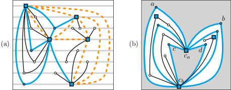
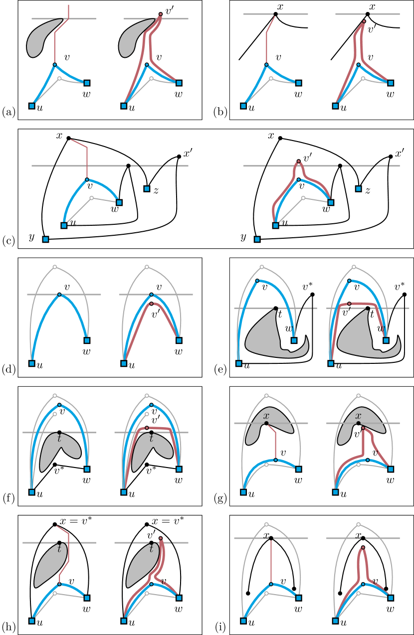
Let be a level planar drawing of a level graph . A visibility edge for is (1) a y-monotone curve that joins two vertices of and can be inserted into without creating any crossings (but possibly a pair of parallel edges); or (2) a horizontal segment that joins two consecutive vertices on a common level of and can be inserted into without creating any crossings. A visibility extension of with respect to a vertex set is a drawing derived from by inserting a maximal set of pairwise non-crossing visibility edges incident only to vertices of such that for each pair of parallel edges in there is at least one vertex of in the interior of the simple closed curve formed by and ; for an illustration see Figure 1(a). We remark that if , then is essentially an interior triangulation containing . However, we will always choose to be a (small) vertex cover, resulting in a much sparser yet still connected augmentation:
Cores and refined visibility extensions.
Intuitively, the core of a level planar drawing is a subset of the vertex set with certain crucial properties. To define it formally, we will first classify the ears of the drawing according to several categories. The concepts introduced in this paragraph are illustrated in Figure 1(b). Let be a level graph, let be a vertex cover of , and let be a level planar drawing of . Consider an ear with neighbors where . If , we say that is a top ear. Otherwise (if ), we say that is a bottom ear. Assume that and that is a top ear. If in the edge is drawn to the left (right) of , we say that is a left (right) ear in . The terms “left” and “right” are defined analogously for bottom ears. If , we consider to be a left ear if it is a top ear; otherwise it is a right ear. Consider a pair with at least one left ear in and let denote the subdrawing of induced by the set of edges that are incident to at least one left ear of in . Note that either all these ears are top ears or all these ears are bottom ears in , and they are arranged in a nested fashion. In case of top (bottom) ears, we refer to the unique one with the largest (smallest) y-coordinate as the outermost left ear of . The innermost left ear of is defined symmetrically. If has an interior (i.e., bounded) face such that the open region enclosed by the boundary of contains a vertex of in , then we say that the two ears on the boundary of are bounding ears of in with respect to . Moreover, we say that are a pair of matching bounding ears whose region corresponds to . The terms “outermost”, “innermost” and “(region of matching pair of) bounding ears” are analogously defined for the right ears of . Every vertex of that is an outermost, innermost, or bounding ear (with respect to some pair ) is called crucial with respect to .
The core of with respect to is the (unique) subset of that contains , , as well as all crucial ears of with respect to . The subdrawing of a visibility extension of with respect that is induced by the core of with respect to captures crucial structural properties of , which we will exploit in our main algorithm for constructing constrained level planar drawings in FPT-time. Due to the fact that has only vertices and edges, it is not difficult to “guess” in XP-time (via the process of exhaustive enumeration) when given and . The main bottleneck is the enumeration of all possible sets of crucial ears. To improve the runtime of this step to FPT-time, we will now describe a variant of visibility extensions that contains some additional ears, which take over the role of the original crucial vertices. Loosely speaking, one can create such a drawing by placing one or two new ears near each crucial ear in a visibility extension. The resulting augmentation retains the helpful structural properties of its underlying visibility extension and we will see that the (positions of the) crucial vertices of some such augmentation can be guessed more efficiently since we can restrict the possible levels of these new vertices to a small set. Formally, a refined visibilty extension of is a crossing-free drawing of a level graph such that is a subgraph of , is a vertex cover of , every vertex in is an ear with respect to and its incident edges are drawn as y-monotone curves, the subdrawing of induced by is a visibility extension of , the crucial ears of are precisely the vertices in , and .
Lemma 3.2 (\IfAppendix).
Let be a level graph without isolated vertices, let be a vertex cover of , let be a level planar drawing of , let be a refined or non-refined visibility extension of with respect to , and let the subdrawing of induced by the core of with respect to . Then is connected and has vertices and edges, where .
4 Algorithm
In this section, we describe the algorithm corresponding to the proof of Theorem 1.1. Let be a constrained level graph and let be a vertex cover of . Our goal is to construct a constrained level planar drawing of or correctly report that such a drawing does not exist. In view of Lemma 2.3, we may assume that has no isolated vertices. To construct the desired drawing, we proceed in three main steps. In Step 1, we “guess” a core-induced subdrawing of a refined visibility extension of a constrained level planar drawing of with respect to (via the process of exhaustive enumeration). In Step 2, we augment our drawing by inserting the transition vertices of with respect to . In Step 3, we finalize our drawing by inserting the leaves and ears of with respect to .
Step 1: Guessing a core-induced subdrawing.
Assume that there is a constrained level planar drawing of , let be a refined visibility extension of with respect to , and let be the subdrawing of induced by the core of with respect to . The procedures corresponding to Steps 2 and 3 of our algorithm are guaranteed to produce a constrained level planar drawing (not necessarily ) of when given . Hence, the goal of Step 1 is to determine (or, rather, guess) , given and . More precisely, we will construct a set of drawings such that and the number of drawings in is sufficiently small. For each drawing in , we then apply Steps 2 and 3 of the algorithm (incurring a factor of in the total running time). Given that , one of the iterations is guaranteed to terminate with a constrained level planar drawing of .
Lemma 4.1 (\IfAppendix).
Let be a constrained level graph without isolated vertices, let be a vertex cover of , and let be a constrained level planar drawing of . There is an algorithm that, given and , constructs a set of drawings in time, where and , such that all drawings in have size and are level planar drawings of subgraphs of induced by and that respect and the orderings and are augmented by some visibility edges and additional ears (with respect to ). Further, there exists a refined visibility extension of such that the subdrawing of induced by the core of with respect to is contained in .
Proof 4.2 (Proof sketch).
We introduce the following terminology: let be a vertex in a level planar drawing (possibly augmented by some horizontal edges). Let be the y-coordinate of and let be the largest y-coordinate of a vertex below (if there no such vertex, we set ). We say that the line is directly below . The line directly above is defined symmetrically.
We proceed in two main steps. In the first main step, we show that there exists a refined visibility extension of . To this end, we start with a visibility extension of and describe an incremental strategy that performs a total of augmentation steps, in each of which a new ear is added that takes over the role of a crucial ear in . (The description of this first main step is deferred to the appendix.) In the second main step, we discuss the construction of the desired family . To this end, let be the subdrawing of induced by the core of with respect to . The drawing is uniquely described by , , the set of visibility edges of (and ), the set of crucial ears of (and ) together with their level assignments and their incident edges, and a compatible edge ordering of the nonhorizontal edges of . The graph , as well as the vertex cover are given, so it suffices to enumerate all possible options for the remaining elements.
There are visibility edges by Lemma 3.2 and each of these visibility edges joins a pair of vertices in . Hence, there are at most possible options for choosing the set of visibility edges. To enumerate the set of crucial ears along with their level assignments, we mimic the aforementioned incremental strategy for constructing : we first enumerate all options to pick the pair of neighbors of the first new vertex along with its level, then, for each of these options, we enumerate all options to pick the pair of neighbors of the the second vertex along with its level, etc., until we have obtained all options to pick the desired vertices together with their levels. More precisely, suppose we have already enumerated all options to pick the first vertices together with their neighbors and levels. For each of these options, to enumerate all options to pick the next vertex , we go through all ways to pick its two neighbors and through all ways to pick the level of . There are pairs of vertices in with ears (by Lemma 3.2). To bound the number of ways to pick the level of , we make use of the fact that whenever the incremental strategy for constructing places a new vertex , it is assigned to a new level directly above or below a level of one of the following categories:
-
•
a level with a vertex in ( possibilities),
-
•
a level with a vertex in ( possibilities by Corollary 2.2),
-
•
a level of a vertex that does not belong to , i.e., a level used for one of the already placed vertices ( possibilities),
-
•
a level with a top-most or bottom-most vertex of ( possibilities),
-
•
a level with a top-most top ear, a top-most bottom ear, a bottom-most top ear, or a bottom-most bottom ear of some pair of vertices in ( possibilities by Lemma 3.2),
-
•
a level with a top-most or bottom-most vertex of a connected component that contains a vertex of in the graph obtained by removing and from the current graph ( together with the visbility edges and the already added vertices) ( possibilities).
In total, for a fixed pair of neighbors , there are thus options to pick a level for . We immediately discard level assignments for which is no ear. By multiplying with the number of ways to choose the neighbors, we obtain options to choose and its level. Multiplying the number of options for all steps together, we obtain a total number of ways to create the set of crucial ears along with their levels. By multiplying with the number of ways to choose the visibility edges, we obtain a total of options to choose the graph that corresponds to . For each of these options we enumerate all permutations of the set of non-horizontal edges and, interpreting the permutation as a compatible edge order, try to construct a level planar drawing for which this order is compatible (cf. Section 2). If we succeed, we check whether the drawing is conform with and can be augmented with the horizontal visibility edges. If so, we include the drawing in the set of reported drawings. The size of the thereby constructed set is bounded by and it is guaranteed to contain by construction.
Step 2: Inserting transition vertices.
We now describe how to insert the transition vertices into the core-induced subdrawing of the (refined) visibility extension . Our plan is to first show that in , every transition vertex is placed “very close to” some visibility edge. Intuitively, this means that the visibility edges of act as placeholders near which the transition vertices have to be placed. We will describe a procedure that does so while carefully taking into account the given partial orderings and prove its correctness by means of an (somewhat technical) exchange argument. To formalize the notion of “very close to”, let be an edge of a level planar drawing joining two vertices such that there is a degree-2 vertex with neighbors and where is the level assignment. We say that is drawn in the vicinity of with respect to a vertex set if the simple closed curve formed by and the two edges incident to does not contain a vertex of in its interior.
Lemma 4.3 (\IfAppendix).
Let be a constrained level graph without isolated vertices, let be a vertex cover of , let be a constrained level planar drawing of , let be a refined or non-refined visibility extension of with respect to , and let the subdrawing of induced by the core of with respect to . There is an algorithm that, given , and , inserts all transition vertices (and their incident edges) into vicinities (with respect to ) of visibility edges in in polynomial time such that the resulting drawing can be extended to a drawing whose restriction to is a constrained level planar drawing of .
Step 3: Inserting leaves and ears.
In this step, we start with the output of Step 2 and finalize our drawing by placing all the vertices that are still missing.
Lemma 4.4.
Let be a constrained level graph without isolated vertices, let be a vertex cover of , let be a constrained level planar drawing of , let be a refined or non-refined visibility extension of with respect to in which each transition vertex is placed in the vicinity of some visibility edge with respect to , and let () be the subdrawing of induced by the core (and the transition vertices) of with respect to . There is an algorithm that, given , , and , extends to a drawing whose restriction to is a constrained level planar drawing of in time, where .
Proof 4.5.
The only vertices of that are missing in are the leaves and the non-crucial ears with respect to (in case is a refined visibility extension, the non-crucial ears are exactly the ears of ). Our plan to insert them into our drawing is as follows. We begin by introducing more structure in and by adding some additional visibility edges and making some normalizing assumptions, which will simplify the description of the upcoming steps. In particular, this step will ensure that for each missing ear, there are essentially only (up to) two possible placements, which will allow us to enumerate all possible ear placements (so-called ear orientations) on a given level in FPT-time. We then describe a partition of the plane into so-called cells in a way that is very reminiscent of the well-known trapezoidal decomposition from the field of computational geometry, cf. [11]. We merge some cells into so-called channels, which correspond to connected y-monotone regions in which the missing leaves along with their incident edges will be drawn (a region is y-monotone if its intersection with every horizontal line is connected). We then introduce (and describe an enumerative process that constructs in FPT-time) a so-called traversal sequence that is compatible with , which is a sequence of sets of channels with several useful structural properties related to . In particular, this sequence, in some sense, sweeps the plane from left to right in a way where for each edge incident to a leaf in , at some point there is a channel that contains it. Exploiting the properties of the traversal sequence, we then describe how to construct a so-called insertion sequence for the leaves on a given level with respect to a given placement of the ears of that level in polynomial time. Such an insertion sequence does not necessarily exist for every placement of ears, but we are guaranteed to find one by enumerating all possible ear placements of the level. This computation is performed independently for each level. Finally, we show how to construct in polynomial time the desired drawing when given an insertion sequence along with its ear placement for each level. Notably, the final step can be executed even if some of the ear placements are different from the ones used in . Let us proceed to formalize these ideas.
Augmenting and normalizing , , and .
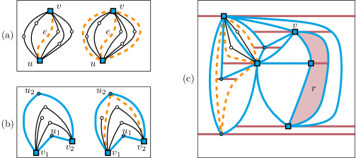
Let be a visibility edge of (and ) that has at least one transition vertex in its vicinity. In both and , we add two copies of ; one directly to the left of the leftmost transition vertex and the other directly to the right of the rightmost transition vertex in the vicinity of , which is possible to do in a y-monotone fashion and without introducing any crossings; see Figure 2(a). Note that the region enclosed by these two edges only contains transitions vertices of and , as well as leaves of or . We repeat this operation for all visibility edges .
The following steps are illustrated in Figure 2(b). Let be a face of that is bounded by four vertices where and are either both left ears or both right ears. Without loss of generality, assume they are both left ears with . We add copies of the edges and in in both and , which can be done without introducing crossings. These edges partition into three regions. Note that in these regions only contain leaves and non-crucial ears. Without loss of generality, we will assume that each leaf in is either placed in the region bounded by and its copy or the region bounded by and its copy (note that a leaf that is adjacent to cannot have a constraint of the form , where is a non-crucial ear in ; the situation for leaves adjacent to is symmetric). Thus, the remaining (central) third region only contains non-crucial ears and is henceforth called an ear-face of . We repeat this modification for all faces such as .
For the remainder of the proof, and are used to refer to the thusly augmented and normalized drawings. We also add all the new edges to and use to refer to this augmentation. Note that this implies that it now suffices to search for a drawing of in which every non-crucial ear is placed in an ear-face, whereas no leaf is placed in an ear-face.
Decomposition into cells.
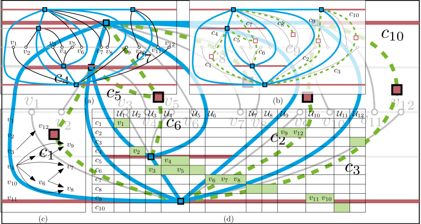
We will now describe a partition of the plane that essentially corresponds to a trapezoidal decomposition (cf. [11]) of ; for illustrations refer to Figure 2(c): for each vertex in , shoot a horizontal ray from to the left until hitting an edge or vertex of , then add the corresponding segment to . In case the ray does not intersect any part of , add the ray itself to . Perform a symmetric augmentation by shooting a horizontal ray from to the right. The maximal connected regions of the resulting partition of the plane are henceforth called cells. We consider the cells to be closed. Note that each cell is y-monotone and bounded by up to two horizontal segments or rays and up to two y-monotone curves. By Lemma 3.2, has vertices and edges (note that the augmentation step copies each edge at most twice) and, hence, it has faces. Consequently, the number of cells is also since the insertion of a single segment or ray can only increase the number of faces (or, rather, maximal connected regions) by one.
Channels.
Let , let be a set of cells that do not belong to ear-faces, and let . Further, assume that contains a cell that is incident to . The triple is a channel from to if it is possible to draw a y-monotone curve in in the interior of the union of that intersects each cell in and does not cross any edge of ; as illustrated in Figure 2(c). We say that can be used by a leaf and that the edge incident to can be drawn in if can be drawn in in the union of without any crossings and there is no channel with this property for which . Further, we say that is used by if it can be used by and the edge incident to is drawn in the union of in . We use to denote the set of all channels and to denote the set of all channels that are used. The connectivity of (cf. Lemma 3.2) can be used to show:
Traversal sequences.
Let be a sequence of sets of channels. We say is a traversal sequence if the following properties are fulfilled (see Figure 3 for illustrations):
-
(T1)
Let and let and with . Then the intersection of the line with the interior of the union of is empty.
-
(T2)
Let be a channel and let be two indices such that and . Then for every , .
We say a channel is active in if it is contained in it, and otherwise it is inactive in it. We say a traversal sequence is compatible with if the following conditions are satisfied (refer again to Figure 3 for illustrations):
-
(C1)
For every channel , there exists an such that if and only if is used.
-
(C2)
There exists a compatible edge ordering for the restriction of to its nonhorizontal edges (recall that some visibility edges are horizontal) such that:
-
(a)
Let be two edges that are incident to leaves and where , let be the channel used by , and let be the channel used by . Then there exist indices such that and , .
-
(b)
Let such that for every edge using and for every edge using we have . Then there is no index such that contains both and (and every index for which is active is smaller than every index where is active).
-
(c)
For every pair of used channels , such that is being used by an edge that succeeds all edges that use in there exists an index such that and (and is active for some index smaller than ).
-
(a)
Ear orientations.
Let and let be all non-crucial ears on the th level. Further, consider a mapping . We say that is an ear orientation of level . We say that is valid if it is possible to insert the ears (on the line ) along with their incident edges into such that the resulting drawing is crossing-free, no constraint is violated (i.e., if , then is placed to the left of ), and for every , we have that is a left ear if and only if . We say that is induced by . Note that for any ear there is at most one left ear-face and at most one right ear-face into which it can be inserted without introducing crossings. Hence, a valid ear orientation uniquely describes the ear-face in which each ear is placed. Further, note that no two ears of can be placed in the same ear-face without introducing crossings. In contrast, whenever an ear orientation assigns only one ear to a given ear-face, it is possible to place the ear without introducing crossings. These properties make it easy to test whether a given ear orientation is valid and, if so, construct the (unique) induced drawing in polynomial time. In view of Lemma 2.4, this means we can enumerate all valid ear orientations of a given level in time.
Insertion sequences.
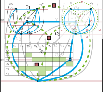
Let be a traversal sequence that is compatible with . Further, let , let be a valid ear orientation of level , and let be its induced drawing. Finally, let be a sequence with , , and for all . We say is an insertion sequence for , , and if the following conditions are fulfilled (for an example, see Figure 4):
-
(I1)
Let . Then there exists at most one index such that .
-
(I2)
Let and with . Then .
-
(I3)
Let . Then there exists a channel that can be used by .
-
(I4)
Let . Then for every with , there exists an index such that .
-
(I5)
Let and let be the (unique, by 3) channel usable by in . Then for every that is not a transition vertex in and where , is to the right of or on the right boundary of . Symmetrically, for every that is not a transition vertex in and where , is to the left of or on the left boundary of .
Let be an insertion sequence for , , and . We say a leaf is choosable with regard to if (i) there exists an index , such that is an insertion sequence for , , and as well and (ii) there exists no pair , with and such that is an insertion sequence.
Claim 4 (\IfAppendix).
Let be a traversal sequence that is compatible with and let be a compatible edge ordering for the restriction of to its nonhorizontal edges, for which Property (C2) is fulfilled for . Further, let and let be the valid ear orientation of level that is used in . For every , there exists an insertion sequence for , , and such that the following two properties are satisfied (for an example, see Figure 4):
Interval property: For every vertex there exists at most one nonempty maximal interval where such that is choosable with regard to if and only if . If such an interval exists, then or . Conversely, if occurs in some entry of , then the interval exists.
Dominance property: Let be the restriction of to edges incident to leaves on level . Further, let , let , and let () be the edge incident to (). Then, if or , we have , where is the maximum index such that the channel used by (in ) is in .
Moreover, is a prefix of for all . Finally, there is an algorithm that, given , , , , and , computes in polynomial time.
Computing the drawing.
When given a traversal sequence that is compatible with , we can utilize 4 to obtain a valid ear orientation together with an insertion sequence for a given level by simply trying to apply the algorithm corresponding to 4 for all valid ear orientations of that level. We do so for each level and then use the gathered information to construct the desired drawing by means of the following claim. We remark that when the algorithm corresponding to 4 successfully terminates, it is guaranteed to return an insertion sequence for the given valid ear orientation. It might output an insertion sequence even if the given valid ear orientation is not the one used in . However, this does not invalidate our strategy as the following claim does not require that the given ear orientations are the ones used in .
Claim 5 (\IfAppendix).
There is an algorithm that, given , , , , a traversal sequence that is compatible with , and, for each level , a valid ear orientation , as well as an insertion sequence for , , and such that (that is, contains all leaves of level ), computes an extension of whose restriction to is a constrained level planar drawing of in polynomial time.
Wrap-up.
In the beginning of (and throughout the) proof of Lemma 4.4, we have already sketched how the individual pieces of the proof fit together. We formally summarize our strategy in the proof of the following claim.
Claim 6 (\IfAppendix).
There is an algorithm that, given , , and , extends to a drawing whose restriction to is a constrained level planar drawing of in time.
This concludes the proof of Lemma 4.4.
Summary.
In the beginning of Section 4, we have already sketched how Lemmas 2.3, 4.1, 4.3 and 4.4 can be combined to obtain Theorem 1.1. We formally summarize:
Theorem 4.6 (\IfAppendix).
There is an algorithm that, given a constrained level graph and a vertex cover of , either constructs a constrained level planar drawing of or correctly reports that such a drawing does not exist in time , where and .
Given that a smallest vertex cover can be obtained in FPT-time with respect to its size [10], our main result (Theorem 1.1) follows from Theorem 4.6.
5 Discussion
We have shown that CLP is FPT when parameterized by the vertex cover number. A speed-up to polynomial time or a generalization to the smaller graph parameters (in particular, tree-depth, path-width, tree-width, and feedback vertex set number) is not possible, even if restricting to OLP or proper CLP instances.
Recall from Section 1 that in the Level Planarity variant Partial Level Planarity (PLP), a given level planar drawing of a subgraph of the input graph has to be extended to a full drawing of , which can be seen as a generalization of OLP and, in the proper case, a specialization of CLP. An instance of PLP can always be turned into an equivalent proper instance (and, thus, a CLP instance) by subdividing each edge on each level it passes through. However, in general this operation will (dramatically) increase the vertex cover number of the instance. Hence, our techniques cannot (directly) be applied. It thus is an interesting problem to study the parameterized complexity of PLP with respect to the vertex cover number.
References
- [1] Patrizio Angelini, Giordano Da Lozzo, Giuseppe Di Battista, Fabrizio Frati, Maurizio Patrignani, and Ignaz Rutter. Beyond level planarity. In Yifan Hu and Martin Nöllenburg, editors, Graph Drawing and Network Visualization - 24th International Symposium, GD 2016, Athens, Greece, September 19-21, 2016, Revised Selected Papers, volume 9801 of Lecture Notes in Computer Science, pages 482–495. Springer, 2016. doi:10.1007/978-3-319-50106-2_37.
- [2] Patrizio Angelini, Giordano Da Lozzo, Giuseppe Di Battista, Fabrizio Frati, and Vincenzo Roselli. The importance of being proper: (in clustered-level planarity and t-level planarity). Theor. Comput. Sci., 571:1–9, 2015. doi:10.1016/j.tcs.2014.12.019.
- [3] Andrei Asinowski, Tillmann Miltzow, and Günter Rote. Quasi-parallel segments and characterization of unique bichromatic matchings. Journal of Computational Geometry, 6:185–219, 2015. arXiv:1302.4400, doi:10.20382/jocg.v6i1a8.
- [4] Christian Bachmaier, Franz-Josef Brandenburg, and Michael Forster. Radial level planarity testing and embedding in linear time. J. Graph Algorithms Appl., 9(1):53–97, 2005. URL: http://jgaa.info/accepted/2005/BachmaierBrandenburgForster2005.9.1.pdf.
- [5] Christian Bachmaier and Wolfgang Brunner. Linear time planarity testing and embedding of strongly connected cyclic level graphs. In Dan Halperin and Kurt Mehlhorn, editors, Algorithms - ESA 2008, 16th Annual European Symposium, Karlsruhe, Germany, September 15-17, 2008. Proceedings, volume 5193 of Lecture Notes in Computer Science, pages 136–147. Springer, 2008. doi:10.1007/978-3-540-87744-8_12.
- [6] Michael J. Bannister, William E. Devanny, Vida Dujmović, David Eppstein, and David R. Wood. Track layouts, layered path decompositions, and leveled planarity. Algorithmica, 81(4):1561–1583, 2019. doi:10.1007/S00453-018-0487-5.
- [7] Václav Blažej, Boris Klemz, Felix Klesen, Marie Diana Sieper, Alexander Wolff, and Johannes Zink. Constrained and ordered level planarity parameterized by the number of levels. In Wolfgang Mulzer and Jeff M. Phillips, editors, 40th International Symposium on Computational Geometry, SoCG 2024, LIPIcs. Schloss Dagstuhl - Leibniz-Zentrum für Informatik, 2024. To appear. URL: https://doi.org/10.48550/arXiv.2403.13702.
- [8] Guido Brückner and Ignaz Rutter. Partial and constrained level planarity. In Philip N. Klein, editor, Proceedings of the Twenty-Eighth Annual ACM-SIAM Symposium on Discrete Algorithms, SODA 2017, Barcelona, Spain, Hotel Porta Fira, January 16-19, pages 2000–2011. SIAM, 2017. doi:10.1137/1.9781611974782.130.
- [9] Guido Brückner and Ignaz Rutter. An spqr-tree-like embedding representation for level planarity. In Yixin Cao, Siu-Wing Cheng, and Minming Li, editors, 31st International Symposium on Algorithms and Computation, ISAAC 2020, December 14-18, 2020, Hong Kong, China (Virtual Conference), volume 181 of LIPIcs, pages 8:1–8:15. Schloss Dagstuhl - Leibniz-Zentrum für Informatik, 2020. doi:10.4230/LIPIcs.ISAAC.2020.8.
- [10] Marek Cygan, Fedor V. Fomin, Lukasz Kowalik, Daniel Lokshtanov, Dániel Marx, Marcin Pilipczuk, Michal Pilipczuk, and Saket Saurabh. Parameterized Algorithms. Springer, 2015. doi:10.1007/978-3-319-21275-3.
- [11] Mark de Berg, Otfried Cheong, Marc J. van Kreveld, and Mark H. Overmars. Computational geometry: algorithms and applications, 3rd Edition. Springer, 2008.
- [12] N. G. de Bruijn. Problems 17 and 18. Nieuw Archief voor Wiskunde, 2:67, 1954. Answers in Wiskundige Opgaven met de Oplossingen 20:19–20, 1955.
- [13] Giuseppe Di Battista and Enrico Nardelli. Hierarchies and planarity theory. IEEE Trans. Systems, Man, and Cybernetics, 18(6):1035–1046, 1988. doi:10.1109/21.23105.
- [14] Vida Dujmović, Michael R. Fellows, Matthew Kitching, Giuseppe Liotta, Catherine McCartin, Naomi Nishimura, Prabhakar Ragde, Frances A. Rosamond, Sue Whitesides, and David R. Wood. On the parameterized complexity of layered graph drawing. Algorithmica, 52(2):267–292, 2008. doi:10.1007/S00453-007-9151-1.
- [15] Michael Forster and Christian Bachmaier. Clustered level planarity. In Peter van Emde Boas, Jaroslav Pokorný, Mária Bieliková, and Julius Stuller, editors, SOFSEM 2004: Theory and Practice of Computer Science, 30th Conference on Current Trends in Theory and Practice of Computer Science, Merin, Czech Republic, January 24-30, 2004, volume 2932 of Lecture Notes in Computer Science, pages 218–228. Springer, 2004. doi:10.1007/978-3-540-24618-3_18.
- [16] Radoslav Fulek, Michael J Pelsmajer, Marcus Schaefer, and Daniel Štefankovič. Hanani–Tutte, monotone drawings, and level-planarity. In Thirty Essays on Geometric Graph Theory, pages 263–287. Springer, 2013. doi:10.1007/978-1-4614-0110-0_14.
- [17] Michael R Garey and David S Johnson. Computers and Intractability: A Guide to the Theory of NP-Completeness. W. H. Freeman & Co., 1990.
- [18] Ashim Garg and Roberto Tamassia. On the computational complexity of upward and rectilinear planarity testing. SIAM J. Comput., 31(2):601–625, 2001. doi:10.1137/S0097539794277123.
- [19] Leonidas J. Guibas and F. Francis. Yao. On translating a set of rectangles. In Proc. 12th Annual ACM Symposium Theory of Computing (STOC 1980), pages 154–160, 1980. doi:10.1145/800141.804663.
- [20] Leonidas J. Guibas and F. Francis. Yao. On translating a set of rectangles. In F. P. Preparata, editor, Computational Geometry, volume 1 of Advances in Computing Research, pages 61–77. JAI Press, Greenwich, Conn., 1983.
- [21] Lenwood S. Heath and Sriram V. Pemmaraju. Recognizing leveled-planar dags in linear time. In Franz-Josef Brandenburg, editor, Graph Drawing, Symposium on Graph Drawing, GD ’95, Passau, Germany, September 20-22, 1995, Proceedings, volume 1027 of Lecture Notes in Computer Science, pages 300–311. Springer, 1995. doi:10.1007/BFb0021813.
- [22] Lenwood S. Heath and Arnold L. Rosenberg. Laying out graphs using queues. SIAM J. Comput., 21(5):927–958, 1992. doi:10.1137/0221055.
- [23] Seok-Hee Hong and Hiroshi Nagamochi. Convex drawings of hierarchical planar graphs and clustered planar graphs. J. Discrete Algorithms, 8(3):282–295, 2010. doi:10.1016/j.jda.2009.05.003.
- [24] Michael Jünger, Sebastian Leipert, and Petra Mutzel. Pitfalls of using PQ-trees in automatic graph drawing. In Giuseppe Di Battista, editor, Graph Drawing, 5th International Symposium, GD ’97, Rome, Italy, September 18-20, 1997, Proceedings, volume 1353 of Lecture Notes in Computer Science, pages 193–204. Springer, 1997. doi:10.1007/3-540-63938-1_62.
- [25] Michael Jünger, Sebastian Leipert, and Petra Mutzel. Level planarity testing in linear time. In Sue Whitesides, editor, Graph Drawing, 6th International Symposium, GD’98, Montréal, Canada, August 1998, Proceedings, volume 1547 of Lecture Notes in Computer Science, pages 224–237. Springer, 1998. doi:10.1007/3-540-37623-2_17.
- [26] Boris Klemz. Convex drawings of hierarchical graphs in linear time, with applications to planar graph morphing. In Petra Mutzel, Rasmus Pagh, and Grzegorz Herman, editors, Proc. 29th Ann. Europ. Symp. Algorithms (ESA’21), volume 204 of LIPIcs, pages 57:1–57:15. Schloss Dagstuhl – Leibniz-Zentrum für Informatik, 2021. doi:10.4230/LIPIcs.ESA.2021.57.
- [27] Boris Klemz and Günter Rote. Ordered level planarity and its relationship to geodesic planarity, bi-monotonicity, and variations of level planarity. ACM Trans. Algorithms, 15(4):53:1–53:25, 2019. Conference version in Proc. GD’17. doi:10.1145/3359587.
- [28] Ignaz Rutter. Personal communication, 2022.
- [29] Andreas Wotzlaw, Ewald Speckenmeyer, and Stefan Porschen. Generalized -ary tanglegrams on level graphs: A satisfiability-based approach and its evaluation. Discrete Applied Mathematics, 160(16-17):2349–2363, 2012. doi:10.1016/j.dam.2012.05.028.
Appendix A Material omitted from Section 2 (Preliminaries)
See 2.3
Proof A.1.
For each level , the drawing induces a linear order on that extends . Consider the order . We claim that is a partial order, implying that the desired drawing can be obtained by performing a topological sort on each level.
To prove the claim, assume towards a contradiction that contains a cycle of the form . Without loss of generality, we may assume that contains no cycle involving fewer vertices. Since and are partial orders, the cycle contains at least one isolated vertex and at least one non-isolated vertex. Without loss of generality, we may assume that is isolated and is non-isolated. Let () be the largest index such that are all isolated. Since only involves non-isolated vertices, it follows that and, further, that since is a partial order. However, this implies that is a cycle in involving fewer vertices than ; a contradiction. So indeed, is a partial order, as claimed.
See 2.4
Proof A.2.
Let . We will use a charging argument to show that contains at most ears. To this end, let denote the subdrawing of that contains only the ears in , as well as all vertices in . Let be a vertex in that is closest to the line . By planarity, this vertex can be adjacent to at most two ears of . We charge these ears to and then delete them, as well as from . We repeat this strategy until all vertices in (and, thus, all ears in ) have been deleted. Every ear is charged to exactly one vertex in and every vertex in is charged at most twice, which implies the claim.
Appendix B Material omitted from Section 3 (Visibility extensions and cores)
See 3.1
Proof B.1.
We begin by proving the connectivity of . Let denote the (level planar) subdrawing of that is induced by the non-horizontal edges. Let be a sequence of edges corresponding to a compatible edge ordering of . We will show inductively that for each the vertices of the subset of vertices in that are incident to at least one of the edges in belong to the same connected component of , which establishes the connectivity of since .
Clearly the claim holds for . Now let and assume that the claim holds for each . We will show that the claim also holds for . Clearly, this is the case when is incident to a vertex of , so assume otherwise. Let be a vertex of that belongs to . Consider the horizontal ray emanating from to the left. To prove the claim, it suffices to show that belongs to the connected component of that contains .
If intersects only in , then contains a visibility edge that joins with a vertex of incident to (by definition of , is visible from the left in ). In this case, the claim follows since this vertex belongs to .
So assume that intersects not only in . Let denote the first point of that is encountered when traversing from . Since there are no isolated vertices, is located on some edge . Moreover, by definition of , , and , it follows that . The definition of asserts that there is a visibility edge between and a vertex of incident to . The claim follows since this vertex belongs to , which concludes the proof of the connectivity of .
To bound the number of edges, assume that contains at least three edges (otherwise, the statement holds). The drawing may contain parallel edges, however, the definition of and the connectivity of assert that each face of (except for possibly the outer face, which could be bounded by two parallel edges) has at least three edges on its boundary. Consequently, Euler’s polyhedron formula yields that has at most edges (the accounts for the special role of the outer face).
See 3.2
Proof B.2.
We will prove the statement for non-refined visbility extensions; the statement for refined visibility extensions then follows easily by definition. Recall that the core of with respect to is the subset of that contains , , as well as all crucial vertices of with respect to .
Connectivity.
We begin by showing that is connected. By Lemma 3.1, the subdrawing of (and ) that is induced by is connected. Moreover, since is a vertex cover, every vertex of , as well as every crucial vertex is adjacent to some vertex of . Consequently, is connected, as claimed.
Counting crucial vertices.
Recall that the crucial vertices with respect to are the ears that are outermost, innermost, or bounding ears of some pair of vertices of . We will examine the counts of these different types of vertices individually.
Counting outer/innermost ears.
We begin by bounding the number of vertices that are outermost left ears. Let be the set of all these ears. Let be the set of vertices that are adjacent to at least one ear in . We will now construct a graph drawing as follows: the vertex set of is and its vertices are placed exactly as in . Let and let denote the neighbors of . We add an edge between in and use the simple curve formed by and its incident edges in to draw it. This process is repeated for every ear . The resulting drawing has vertices and edges, which are in one-to-one correspondence with the ears in . Moreover, the drawing is by construction planar and has no parallel edges. Hence, Euler’s polyhedron formula implies .
The outermost right and the innermost left/right ears can be bounded analogously, which yields outermost and innermost ears in total.
Counting bounding ears.
To count the number of bounding ears, we will use a charging argument. Consider a matching pair of bounding ears of with region (which, by definition, contains at least one vertex of ). If there is no pair of matching bounding ears whose region is a proper subset of , we charge the pair to an arbitrary vertex of in the interior of . Otherwise, let be an inclusion-maximal region contained in that is the region of a pair of matching bounding ears. The boundary of contains exactly four vertices: and , as well as two vertices of . At least one of the latter two has to be contained in the interior of since , say . Note that is distinct from both and , which belong to the boundary of . We charge the pair to . This charging procedure is repeated for all matching pairs of bounding ears.
The inclusion-maximality of the regions implies that each vertex of gets charged at most once: consider a vertex and assume it is charged by a pair of bounding ears with region . Then is located in the interior of . Suppose there is another pair of bounding ears with region that is charged to . Then is also located in the interior of . By planarity and the fact that is interior to both and , the boundaries of and are nested, leaving two cases: or . In the case , we obtain a contradiction since would have been charged to a vertex that is located on the boundary of or on the boundary of some region with , implying that is distinct from , which is interior to . The case is symmetric. So indeed, each vertex of is charged at most once, as claimed. Moreover, no vertex of the outer (i.e., unbounded) face of can be charged. Since there are at least two vertices of on the outer face (assuming ), we obtain that the number of pairs of matching bounding ears is at most . Consequently, the number of bounding ears is at most .
Wrap-up.
We have shown that the number of crucial vertices is . The number of vertices in is by definition and the number of vertices in is by Corollary 2.2. This yields a total number of vertices in the core of with respect to .
The -bound on the number of visibility edges follows from Lemma 3.1. When removing all visibility edges from , we end up with a drawing without parallel edges. Hence, Euler’s polyhedron formula implies that its number of edges, and therefore the number of edges in , is bounded by .
Appendix C Omitted material from Section 4 (Algorithm)
See 4.1
Proof C.1.
We proceed in two steps. In the first step, we show that there exists a refined visibility extension of such that the set of vertices in that do not belong to only use a restricted (small) set of levels. In the second step, we use the results from the first step to discuss how to construct the desired family .
Existence of .
Towards the first step, let be a visibility extension of . We apply the following normalization: let be a pair of matching bounding ears and let be the common neighbors of . Without loss of generality, assume that the level of is lower than the one of and that are top ears. If the intersection of the region of with the closed upper half-plane bounded by is empty or contains only leaves of , then we redraw all edges of leaves of whose upper endpoint is in such that they intersect directly to the right of and then closely follow towards such that none of them has a vertex in to its left. Similarly, we can now redraw such that it also has no vertex in to its left. We apply a symmetric transformation to the leaves of and the edge . Finally, we insert a maximal set of visibility edges to ensure that the result is again a visibility extension of . We repeat this strategy until the precondition of the redrawing procedure is unfulfilled for every pair of matching bounding ears. A given edge might be redrawn multiple times, however, this procedure is guaranteed to terminate since each edge either moves monotonically to the left or moves monotonically to the right. Overloading our notation, from now on we use to denote the final redrawing.
We will now describe an iterative process that augments (by inserting new ears) to obtain the desired refined visbility extension . Each new vertex created in this process will be placed on a “private” new level (of width ). To facilitate the description of the extended level assignment, we introduce the following terminology: let be a vertex in a level planar drawing (possibly augmented by some horizontal edges). Let be the y-coordinate of and let be the largest y-coordinate of a vertex below (if there no such vertex, we set ). We say that the line is directly below . The line directly above is defined symmetrically.
Suppose we have already performed some number (possibly zero) of augmentation steps and let denote the resulting augmentation of . We now discuss how to perform the next augmentation step. Let be an ear of that is crucial in and let denote its neighbors (if such a vertex does not exist, we are done and is the desired representation ). We describe a procedure that creates up to two new ears to ensure that is no crucial ear of the resulting augmentation of . Without loss of generality, let be a top left ear (the other cases are handled symmetrically). We iteratively consider four cases, which are not mutually exclusive (up to two can occur at the same time).
Case 1.
is an outermost ear. Let be a y-monotone curve whose lower endpoint is , whose interior does not intersect , and whose upper endpoint is either (i) on the line directly above the top-most vertex of or (ii) a vertex of so that is between two incoming edges of . (Such a curve does always exist: it can be constructed by traversing upwards from in a greedy-like fashion.)
If the upper endpoint of is of type (i), we place a new ear of at the upper endpoint of and draw its incident edges by first following to and then either the edge or ; see Figure 5(a).
If the upper endpoint of is of type (ii), then it is a vertex such that either , , or is a top ear of . We distinguish two subcases.
If , , or is the lowest top ear of its two neighbors, we place a new ear of on the intersection of with the line directly below and draw its incident edges by first following to and then either the edge or ; see Figure 5(b).
If is not the lowest top ear of its two neighbors, which we denote by and , we place a new ear of on the intersection of with the line directly above the top-most ear of and draw its incident edges by first following to and then either the edge or ; see Figure 5(c). Note that indeed always intersects : all ears of lie inside the region bounded by the cycle where is the lowest top ear of . It follows that the top-most ear of (and, thus, ) is below since the latter is the topmost point of .
Overloading our notation, from now on (when considering Cases 2–4) we use to denote the resulting drawing in which no longer satisfies the assumption of Case 1.
Case 2.
is an innermost ear. If is a lowest top ear of , we place a new vertex on the line directly below and between the two edges incident to and draw the two incident edges of by following the incident edges of ; see Figure 5(d). Otherwise, there exists an innermost right ear of whose level is lower than the level of (since is an innermost left ear); for illustrations refer to Figure 5(e). Among the vertices that are located in the region bounded by the cycle and that are not leafs of or , let be a top-most vertex (if the region does not contain such a vertex, we set ). Assume without loss of generality that the edge is to the left of the edge . We place a new vertex on the line directly above and between the two edges incident to and to the right of the rightmost edge that is incident to a leaf of (if any) and to the left of the leftmost edge that is incident to a leaf of (if any). We connect to and by going to the left and right until reaching edges. These edges must either be incident to or to a leaf of or . In both cases, we can follow these edges to connect to and .
Overloading our notation, from now on (when considering Cases 3–4) we use to denote the resulting drawing in which no longer satisfies the assumptions of Cases 1–2.
We conclude this case with a small observation that will later help with the construction of the desired family : if , then can neither be a leaf of or nor an ear of and . It follows that in the graph obtained by removing and from there is at least one vertex of in the connected component of . The number of connected components that contain a vertex of is bounded by . Hence, the number of levels with a top-most vertex of one of these components is also bounded by .
Case 3.
There is a vertex such that is a pair of matching bounding ears of in and has a lower level than . Assume without loss of generality that the edge is to the left of the edge ; for illustrations refer to Figure 5(f). Among the vertices that are located in the region bounded by the cycle and that are not leaves of or , let be a top-most vertex. If the level of is above the one of , by our normalizing assumption, we know that is not a vertex of . In this case re-define . We place a new vertex on the line directly above and between the two edges incident to and to the right of the rightmost edge that is incident to a leaf of (if any) and to the left of the leftmost edge that is incident to a leaf of (if any). We connect to and by going to the left and right until reaching edges. These edges must either be incident to or to a leaf of or . In both cases, we can follow these edges to connect to and .
Overloading our notation, from now on (when considering Case 4) we use to denote the resulting drawing in which no longer satisfies the assumptions of Cases 1–3.
Case 4.
There is a vertex such that is a pair of matching bounding ears of in and has a higher level than . Similiar to Case 1, let be a y-monotone curve whose lower endpoint is , whose interior does not intersect , and whose upper endpoint is a vertex of so that is between two incoming edges of . (Such a curve does always exist: it can be constructed by traversing upwards from in a greedy-like fashion.)
If or , we place a new ear of on the intersection of with the line directly below and draw its incident edges by first following to and then either the edge or ; see Figure 5(g).
If , then among the vertices that are located in the region bounded by the cycle and that are not leaves of or , let be a top-most vertex. We place a new ear of on the intersection of with the line directly above and draw its incident edges by first following to and then either the edge or ; see Figure 5(h). Note that indeed always intersects by our normalization procedure (this is true even if does not belong to by construction).
Finally, assume that is a top ear, but at least one of its adjacent vertices is neither nor . Let be the neighbors of . We place a new ear of on the intersection of with the line directly below and draw its incident edges by first following to and then either the edge or ; see Figure 5(i). Note that is a lowest top ear of since is crossing-free.
This concludes the description of Case 4, after which no longer satisfies the assumptions of Cases 1–4.
We repeat this augmentation step until no crucial vertices of are still crucial in yielding the desired refined visibility representation . Note that, by Lemma 3.2, the total number of augmentation steps is .
Construction of .
We are now ready to discuss the construction of the desired family . Let be the subdrawing of induced by the core of with respect to . The drawing is uniquely described by , , the set of visibility edges of (and ), the set of crucial ears of (and ) together with their levels and their incident edges, and a compatible edge ordering of the nonhorizontal edges of . The graph , as well as the vertex cover are given, so it suffices to enumerate all possible options for the remaining elements.
There are visibility edges by Lemma 3.2 and each of these visibility edges joins a pair of vertices in . Hence, there are at most possible options for choosing the set of visibility edges.
To enumerate the set of crucial ears along with their level assignment, we mimic the above construction of : we first enumerate all options to pick the pair of neighbors of the first new vertex along with its level, then, for each of these options, we enumerate all options to pick the pair of neighbors of the the second vertex along with its level, etc., until we have obtained all options to pick vertices together with their levels. More precisely, suppose we have already enumerated all options to pick the first vertices together with their neighbors and levels. For each of these options, to enumerate all options to pick the next vertex , we go through all ways to pick its two neighbors and through all ways to pick the level of . There are pairs of vertices in with ears by Lemma 3.2. To bound the number of ways to pick the level of , recall that whenever the above procedure places a vertex , it is assigned to a new level directly above or below a level of one of the following categories:
-
•
a level with a vertex in ( possibilities),
-
•
a level with a vertex in ( possibilities by Corollary 2.2),
-
•
a level of a vertex that does not belong to , i.e., a level used for one of the already placed vertices ( possibilities),
-
•
a level with a top-most or bottom-most vertex of ( possibilities),
-
•
a level with a top-most top ear, a top-most bottom ear, a bottom-most top ear, or a bottom-most bottom ear of some pair of vertices in ( possibilities by Lemma 3.2),
-
•
a level with a top-most or bottom-most vertex of a connected component that contains a vertex of in the graph obtained by removing and from the current graph ( together with the visbility edges and the already added vertices) ( possibilities by the observation at the end of Case 2).
In total, for a fixed pair of neighbors , there are thus options to pick a level for . We immediately discard level assignments for which is no ear. By multiplying with the number of ways to choose the neighbors, we obtain options to choose and its level. Multiplying the number of options for all steps together, we obtain a total number of ways to create the set of crucial ears along with their levels. By multiplying with the number of ways to choose the visibility edges, we obtain a total of options to choose the graph that corresponds to . For each of these options we enumerate all permutations of the set of non-horizontal edges and, interpreting the permutation as a compatible edge order, try to construct a level planar drawing for which this order is compatible (cf. Section 2). If we succeed, we check whether the drawing is conform with and can be augmented with the horizontal visibility edges. If so, we include the drawing in the set of reported drawings. The size of the thereby constructed set is bounded by and it is guaranteed to contain by construction.
See 4.3
Proof C.2.
The terminology introduced in the following paragraphs is illustrated in Figure 6(a). Let such that there exists at least one transition vertex adjacent to both and , and let denote be the visibility edges joining and in the left-to-right order in which they appear in . These edges partition the open horizontal strip bounded by the lines and into regions where is on the boundary of and .
Let be the connected components of the graph represented by after deleting . Note that these can contain vertices on the boundary or exterior to . However, by planarity, if a component contains a vertex in a region , then all of its vertices are located in in . Similarly, if a component contains a vertex exterior to all of the regions in , then all of its vertices are located exterior to all of the regions . When contains a vertex of in in , then this vertex is drawn in in as well; we say that is fixed to . Additionally, when contains a vertex of that is not located in the open strip , then we consider to be fixed to both and (representing the fact that lies outside of the regions ). In particular, every component that contains at least two vertices also contains a vertex of and is, thus, fixed to some region . Consequently, the only components that are not fixed are the transition vertices of and and the leaves of or (since has no isolated vertices).
The maximality of the set of visibility edges used to construct implies that for each transition vertex of , there exists an index such that there is no fixed component interior to the region bounded by and the two incident edges of , in other words, is drawn in the vicinity of with respect to .
Algorithm.
To obtain from we will draw every transition vertex of in the vicinity of one of the visibility edges of . To this end, we now define several sets and relations, for illustrations refer to Figure 6(b). Let be the set that contains all non-fixed components (i.e. the transition vertices and leaves of and/or ), as well as the components that are fixed to one of the regions . For each region for which contains multiple fixed components, we merge all of these components into a single fixed subgraph and use to denote the resulting set, which consists of one fixed subgraph for each of the regions , as well as the transition vertices and leaves of and/or .
We define a relation on as follows: (with and ) if and only if (1) there exists a vertex in and a vertex in such that or (2) and are fixed subgraphs with fixed to , fixed to and or (3) there exists a such that and .
The relation is by definition transitive, but it is not necessarily a partial order. Nevertheless, we will now describe a strategy to derive a total ordering from that will be useful for placing the transition vertices: suppose contains a cycle of the form of pairwise distinct elements . Assume towards a contradiction that one element of , say , consists of precisely one transition vertex of . In , the incident edges of partition into a left and a right side. An inductive argument shows that all components in the cycle are drawn entirely on the right side, including ; a contradiction. Consequently, all elements of must be fixed subgraphs or leaves. Without loss of generality we may assume that consists of at least two vertices ( cannot consist exclusively of vertices lying on a common level since is a partial order). This implies that is fixed, say, to (). Similarly as before, inductive arguments show that all elements of have to lie to the right of and to the left of , i.e., in . Therefore is the unique fixed component of in (and also the unique fixed component in ). We contract into a single subgraph inheriting all relations imposed by on . In this fashion, we successively eliminate all cycles and eventually obtain an ordering on the resulting set , which admits a linear extension . Observe that ordering of corresponding to is of the form
where denotes the fixed subgraph of in and each is a sequence of transition vertices and leaves of and/or . We remove all elements from that correspond to leaves and denote the resulting set by . Let denote the total order on that corresponds to the restriction of to . Observe that the ordering of corresponding to is of the form
where is the restriction of to the transition vertices. For each we draw in the vicinity of the visibility edge in this order (which can obviously be done without introducing crossings), see Figure 6(c). To obtain the desired drawing , we repeat this procedure for every pair . Clearly, all these steps can be performed in polynomial time.
We remark that it might seem tempting to draw the transition vertices, as well as the leaves according to , instead of just drawing the transition vertices according to . However, this will in general not produce a drawing with the desired properties as there might be leaves affected by constraints of components fixed to and/or , which are not taken into account when computing and , as illustrated in Figure 6(c).
Correctness.
Suppose we have already carried out the above procedure for a set of vertex cover vertex pairs and obtained a drawing that consists of augmented by all transition vertices that belong to some pair in . Assume inductively that can be extended to a drawing, without loss of generality , whose restriction to is a constrained level planar drawing of . Consider a pair in with at least one transition vertex and let denote the drawing derived from by inserting the transition vertices of according to the above procedure. Our goal is to show that can be extended to a drawing whose restriction to is a constrained level planar drawing of . To this end, we will construct a drawing from whose restriction to is a constrained level planar drawing of and whose restriction to the graph represented by is .
Let denote the simple closed curve corresponding to the boundary of the outer face of the subdrawing of induced by the visibility edges joining and and the edges that are incident to some transition vertex of . We use to denote the closed interior of and to denote the open exterior of . Note that all visibility edges joining and and all transition vertices of are located in in and, hence, all visibility edges joining and in are also located in .
To construct from , we augment such that it looks exactly as in . Additionally, we draw the fixed subgraphs exactly as in . Let denote the resulting drawing. To construct from , it remains to describe the placement of the leaves of and (which we call leftover leaves) that are located in in , but do not belong to any fixed subgraph (note that the leaves in in and the leaves in the fixed subgraphs have already been drawn in ), as well as the placement of all the transition vertices of (which are all located in in and, thus, have not yet been drawn in ). To this end, we draw those leftover leaves and transition vertices that occur in the sequence in the vicinity of the visibility edge in the order given by (which can be done without introducing crossings).
Since , the restriction of to the graph represented by corresponds to , as desired. Hence, it remains to argue that the restriction of to is a constrained level planar drawing of . By construction, is a level planar drawing of , so assume that some constraint is violated in , i.e., is drawn to the right of on (instead of to the left, as required). By definition of , the restriction of to its non-visibility edges is a constrained level planar drawing of the corresponding subgraph of . Consequently, one of or is a vertex of that does not belong to , i.e., a leftover leave or transition vertex of and/or , which lies in in . Assume without loss of generality that this vertex is (the other case is symmetric). The definition of implies that lies in and, by assumption, to the right of , which contains . However, by definition of , the vertex also lies to the right of in . Since the vertex also lies in in , it follows that the constraint is also violated in ; a contradiction to the definition of . So indeed, (and, thus, ) satisfies all desired properties, proving the correctness of the algorithm.
See 1
Assume there are two channels with and such that the unique cell in that contains and the unique cells in that contains are identical. Then there exist two cells with above such that it is possible to draw two y-monotone curves that do not cross each other and that do not intersects any edge or vertex of and where the endpoints and of and , respectively, satisfy the following properties:
-
•
belongs to the lower boundary of and the upper boundary of some cell ;
-
•
belongs to the lower boundary of and the upper boundary of some cell ;
-
•
belongs to the upper boundary of and the lower boundary of some cell ;
-
•
belongs to the upper boundary of and the lower boundary of some cell .
By construction, the simple closed curve formed by and and the line segments and intersects no vertex or edge of , has in its exterior, and contains at least one vertex of in its interior. However, the connectivity of (cf. Lemma 3.2) implies that contains a path from to ; a contradiction.
It follows that for every pair of channels with , the unique cell in that contains and the unique cell in that contains are distinct. Consequently, we obtain , where denotes the number of cells incident to for each . Recall that each cell is y-monotone and bounded by up to two horizontal segments or rays and up to two y-monotone curves. Now, let , let denote the number of cells incident to for which is incident to at least one y-monotone curve of the cell boundary, and let denote the number of the remaining cells incident to (where is incident only to horizontal segments or rays of the cell boundary). Observe that . Additionally, each cell can contain at most vertices of that are incident to y-monotone curves along the boundary of . Putting it all together, we obtain
where the final inclusion uses and .
See 2
Let be a compatible edge ordering for the restriction of to its nonhorizontal edges and let be the restriction of to the edges that are incident to leafs. We will now label every used channel with a set of numbers corresponding to the edges that use it in : let be a used channel. We label with the number if and only if the th edge in uses . Note that a channel can be assigned multiple labels. Let be the number of leaves. For every , we define to be all channels labeled with two (not necessarily distinct) fulfilling ; see Figure 3 for examples. Let denote the resulting sequence.
is a traversal sequence.
We will now show that the sequence is a traversal sequence. To show Property (T1), let and let and with . Assume towards a contradiction that the line intersects the interior of the union of . Let denote a cell of that is intersected by and let denote the edge that corresponds to the left boundary of . Assume without loss of generality that lies to the right of . Note that every edge incident to precedes in . Moreover, every edge that intersects the interior of succeeds . Hence, every edge using precedes every edge using in . Since , it contains a label that is at least and, hence, it follows that all labels in are strictly larger than ; a contradiction to the fact that . Therefore, Property (T1) is satisfied.
is compatible with .
We will now show the compatability of with . Let be a used channel. Then there exists at least one edge using in . Let be the index of in . Then, by construction, . Moreover, by construction, does not contain any channels that are not used. Therefore, Property (C1) is satisfied.
To establish Property (C2)a, let be two edges that are incident to leaves with , let be the channel used by in and let be the channel used by in . Let further be the indices of , respectively, in the ordering corresponding to . Then and and by construction and, therefore, Property (C2)a is satisfied.
To establish Property (C2)b, let such that for every edge using and for every edge using , we have . Let be the largest index of an edge in with respect to and let be the smallest index of an edge in with respect to . Note that and, by construction, the interval in which is active ends with and the interval in which is active starts with . Therefore, there is no index at which both and are active and is active before , which establishes Property (C2)b.
To establish Property (C2)c, consider two used channels , such that is being used by an edge that succeeds all edges that use in . Let be the index of with respect to . Then and by construction (and is active before by Property (C2)a), which establishes Property (C2)c. Therefore, is indeed compatible with .
Bounding the length of the sequence.
Note that if there are two consecutive sets in with , then we can remove one of them and the resulting sequence is still a traversal sequence that is compatible with , e.g, in Figure 3 the set can be removed. Repeat this process to eliminate all consecutive pairs of identical sets and denote the resulting sequence by . Since the number of channels in is by 1 and the sets containing a channel form an interval by Property (T2), it follows that the length of is .
Algorithm.
So far, we have shown that there is a constant such that there is a traversal sequence compatible with of length at most . Moreover, we know that there is a constant such that by 1. Every traversal sequence of length at most is uniquely described by specifying for each channel at which index in its interval (cf. Property (T2)) starts and at which index it ends (when the starting index is larger than the ending index, does not appear in the sequence). Hence, there are at most candidate sequences. Testing whether a candidate sequence is a traversal sequence is easily done in polynomial time and the existence of implies that at least one of the sequences is a traversal sequence that is compatible with .
See 3
Assume towards a contradiction that contains two channels and that can be used by . Then there are two cells and such that there is a horizontal line intersecting both and . This implies that the precondition of Property (C2)b is fullfilled and the conclusion of Property (C2)b implies that are not both contains in , which yields the desired contradiction.
See 4
Suppose, inductively, we have obtained insertion sequences for , and such that for each of them the interval and the dominance properties are fulfilled and such that is a prefix of for all . Note that if , then is an insertion sequence with the desired properties. Let , . Our goal is to construct the sequence .
Existence of choosable vertices.
We first show that there is a choosable vertex with regard to . To this end, it suffices to show that there exists at least one pair such that is an insertion sequence for , , and (note that this does not necessarily imply that is choosable, but its existence implies that there is a choosable vertex, as desired).
Let be the left-most leaf on level in that is not contained in and let be the channel used by (in ). Let be the largest index such , which exists by Property (C1). Note that if , the definition of implies that can be appended to the (empty) sequence to obtain an insertion sequence for , , and , as desired. So assume otherwise, i.e., . Let .
Our main goal is now to show that , which is a necessary condition for appending to . Towards a contradiction, assume . Let be the largest index that occurs in and where (if no such index exists, we define ). Let be the largest index such that contains (if , we define ).
We will now argue that can be appended to to obtain an insertion sequence for , and , which we will then use to argue that does not satisfy the interval property, yielding the desired contradtion.
So let be the sequence obtained from by appending . Clearly, Properties (I1), (I2), (I3), and (I5) are satisfied for the sequence . To see that Property (I4) also holds, assume towards a contradiction that there is a vertex with that is not contained in . By the definition of , the vertex is contained in . Without loss of generality, assume that is the first vertex in with these properties. Let .
The constraint implies together with Property (C2)a that there exists an index such that the channel used by (in ) is contained in . To obtain the desired contradiction (to the existence of ), we will now show that is can be appended to to obtain an insertion sequence for , and . Since and , it follows that (by definition of ). Further, since (again by definition of ) there is no index that occurs in and where , it follows that . Due to the dominance property for in , is at most as large as the largest index for which . To summarize, .
By Property (T2) and since and and , it follows that . Then, since is the first vertex in with with that is not contained in , it follows that can be appended to without violating Property (I4) to obtain an insertion sequence for , , and . Moreover, note that where and, hence is not choosable with regard to , which yields a contradiction to the interval property for in . Therefore, the vertex with that is not contained in cannot exists an, hence, Property (I4) is satisfied by , which, finally, shows that is an insertion sequence , and .
Once again, note that where and, hence is not choosable with regard to , which yields a contradiction to the interval property for in . Therefore . The fact that can be combined with the definition of to obtain that is indeed an insertion sequence for , , and , as claimed, and, thus, there exists at least one choosable vertex with regard to .
Interval property.
Now let be a choosable vertex together with an smallest index such that is an insertion sequence for , , and . We will now show that it satisfies the interval property. Let be a vertex. We will show that the interval property is fulfilled for . We distinguish four cases.
Case 1:
. Then, has been choosable in in an interval ending with and , thus the interval property is fulfilled.
Case 2:
. Hence, and, thus, it is not choosable for , and the interval property is fulfilled for since it was already fulfilled in .
Case 3:
The interval in which was choosable in is empty. Then the interval in which is choosable in has length at most one and if it has length exactly one, it is choosable only with regard to , hence, the interval property is fulfilled.
Case 4:
is not contained in and the interval in which was choosable in is nonempty and ends with . We need to show that is choosable with regard to .
There exists a channel in that can be used by since we could have appended with the same index as we included . Further, there exists no constraint of the form or , otherwise one of them would have not been choosable with regard to as appending it would have violated Property (I4) of the resulting insertion sequence. Let denote the sequence obtained by appending to . We claim that is an insertion sequence. Indeed, Property (I1) is fulfilled, since was not in . Property (I2) is fulfilled for since and both were appended with index . We already stated that can use a channel in , therefore, Property (I3) is fulfilled. Property (I4) is fulfilled since was choosable with regard to . Property (I5) is fulfilled for since the unique usable channel in that is used by in does not change. This shows that is still choosable with regard to , and the interval property is fulfilled.
So in any case, the interval property for is fulfilled.
Dominance property.
It is left to show that the dominance property is fulfilled for . For all vertices in but , the dominance property carries over from .
Let and let () be the edge incident to () with or . We have to show that , where is the maximum index such that the channel used by (in ) is in . We distinguish two cases:
Case 1:
. Assume towards contradiction that and let be the largest index such that is present in and (if such an index does not exists, we define ). Further, let be the largest index such that contains index (and if ).
Let be the sequence obtained from by appending . We will show is an insertion sequence for , , and , which gives us a contradiction to the interval property of , where (since it is not choosable with regard to ).
Clearly, Properties (I1), (I2), (I3), and (I5) are fulfilled for . It remains to establish Property (I4). Since is choosable in , all vertices with are already in and, thus, the dominance property is fulfilled for them in . Let be such a vertex, let be the index with which is contained in and let be the edge incident to . Clearly, . Hence, by the dominance property of , it follows (and also since is present in ) and therefore, is contained in . Thus, Property (I4) is also fulfilled and is indeed an insertion sequence. This is a contradiction to the interval property of , where since it is not choosable with regard to . Thus, , as desired.
Case 2:
. Assume towards contradiction that . Because of Case 1, we know that is at most as large as the largest index of the channel used by (in ) and, hence is strictly smaller than this index. Also because of Property (C2)a, we know that there exists an index with and , thus, by Property (T2), we know that .
Now let be the largest index such that is present in and (if such an index does not exists, we define ). Further, let be the largest index such that contains index (and if ). Let be the sequence obtained from by appending . We will show is an insertion sequence for , , and , which gives us the desired contradiction to the interval property of , where (since it is not choosable with regard to ).
Clearly, Properties (I1), (I2), (I3), and (I5) are fulfilled for . It remains to establish Property (I4). Since is choosable in , all vertices with are already in and, thus, the dominance property is fulfilled for them. Let be such a vertex, let be the index with which is contained in and let be the edge incident to . Clearly, . Hence, by the dominance property of , it follows (and also since is present in ) and therefore, is contained in . Thus, Property (I4) is also fulfilled and is indeed an insertion sequence. This is a contradiction to the interval property of , where since it is not choosable with regard to . Thus, , as desired.
Therefore, the dominance property is satisfied.
Algorithm.
We have shown that we can generate by starting with an empty sequence and appending choosable vertices until all leaves of level are contained in the insertion sequence (the insertion sequence illustrated in Figure 4 was created by means of this algorithm). Clearly, testing whether a vertex is choosable can be done in polynomial time, therefore we can generate in polynomial time as well.
See 5
For every level , draw the ears in the unique way described by , which can be done without creating any crossings. Let denote the resulting drawing.
We now add the leaves to according to the insertion sequences as follows. We consider all indices in increasing order. To process an index , we consider all levels in increasing order. To process a level , we consider the indices in increasing order. To process the index , let be the -th entry of the insertion sequence . If , let be unique channel usable by in . If consists of a single cell (namely, ) that contains transition vertices, we just assign to , without drawing it yet. Assigned vertices will be drawn in a post-processing step. Otherwise, i.e., if is not a cell that contains transition vertices , we draw a (nearly horizontal) line from to the right boundary of the union of , then traverse along upwards or downwards along this boundary until we reach the y-coordinate .
Assume that we have already performed some number of steps of the algorithm while maintaining the following invariants:
-
1.
The current drawing is crossing-free;
-
2.
For each level , the leaves already present in the drawing (which do not include the assigned leaves) are in the same order as in ; and
-
3.
Let be a leave that is already present or assigned and let . Further, let be the unique channel usable by in . Then is either drawn in or assigned to .
Let be the tuple that is processed in the next step and let be the unique channel in that can be used by . If consists of a single cell (namely, ) that contains transition vertices, the invariants are obviously maintained. Otherwise, if does not contain transition vertices, the curve along which the algorithm draws the edge incident to is not crossed by any of the previously drawn edges by Property (T1) and Property (C2)b of the traversal sequence and, hence, Invariant 1 is maintained. For Invariant 2, assume towards a contradiction that there is an already inserted leaf that is to the right of . By construction, it is in a cell that is to the right of the one of . This is a contradiction to Property (C2)b. Clearly, Invariant 3 is satisfied.
Hence, the invariants are maintained. Let denote the resulting drawing. It remains to draw the unassigned leaves. For each level and for each cell with transition vertices on level , we simply perform a topological sort with respect to on all vertices in (which are assigned leaves and transition vertices) and then place them according to the obtained order (possibly rearranging the order of the transition vertices in ), which is easy to do without introducing crossings. Let denote the final drawing, which is cross-free.
It remains to show that in all constraints are respected. By construction, this is the case for the vertices in .
So let be a leaf on level , let be the channel used by in . All constraints between and other leaves are respected as all leaves on level appear in the same order as in up to permutations in transition vertex cells according to topological orderings with respect to . Constraints between and non-leafs are satisfied by Property (I5).
Clearly, all steps of the algorithm can be carried out in polynomial time.
See 6
We begin by augmenting as described in the beginning of the proof of Lemma 4.4, which is easy to do in polynomial time. The decomposition into cells can also easily be constructed in polynomial time. We then use 2 to construct a set of candidate traversal sequences of length at most that is guaranteed to contain a traversal sequence that is compatible with in time.
For each of these candidate sequences, we now try to construct a valid ear orientation together with an insertion sequence for each level. To do this for a given level , we enumerate all (at most ) valid ear orientations for level in time. For each of these valid ear orientations, we then try to apply the algorithm corresponding to 4 to obtain an insertion order, which takes polynomial time per ear orientation. If we succeed in finding a valid ear orientation together with an insertion sequence for each level, we now try to apply the algorithm corresponding to 5 to construct the desired drawing, which takes polynomial time. If we fail at any point along the way, we just continue with the next candidate traversal sequence.
Since our candidate set contains a traversal sequence that is compatible with , we are guaranteed to eventually obtain the desired drawing. In particular, when applying our strategy to the compatible sequence, we are guaranteed to obtain a valid ear orientation (not necessarily the one used in ) together with an insertion sequence for each level, which allows us to successfully apply the algorithm corresponding to 5. We remark that if the algorithm corresponding to 5 successfully terminates, it is guaranteed to return an insertion sequence for the given valid ear orientation. Moreover, we emphasize that 5 does not require that the ear orientations are the ones used in , meaning that our strategy is not invalidated by the fact that algorithm corresponding to 4 might output an insertion sequence even if the given valid ear orientation is not the one used in . The total runtime of the algorithm is , as claimed.
See 4.6
Proof C.3.
In view of Lemma 2.3, we may assume that has no isolated vertices. Assume that there is a constrained level planar drawing of . We begin by applying Lemma 4.1, that is, we construct a family of drawings for which there exists a refined visibility extension of such that the subdrawing of induced by the core of with respect to is contained in . For each drawing in , we try to apply the algorithm corresponding to Lemma 4.3 to insert the transition vertices in polynomial time. If successful, we then try to apply the algorithm corresponding to Lemma 4.4 to construct the desired drawing in time. If successful, we report the drawing. If we fail at any point along the way, we just continue with the next drawing in . Given that contains , we are guaranteed to eventually obtain the desired drawing. In contrast, if does not admit a constrained level planar drawing, the described algorithm is guaranteed to fail in every iteration, in which case we correctly report that the desired drawing does not exists. The total runtime is .