Tverberg’s theorem and multi-class support vector machines
Abstract.
We show how, using linear-algebraic tools developed to prove Tverberg’s theorem in combinatorial geometry, we can design new models of multi-class support vector machines (SVMs). These supervised learning protocols require fewer conditions to classify sets of points, and can be computed using existing binary SVM algorithms in higher-dimensional spaces, including soft-margin SVM algorithms. We describe how the theoretical guarantees of standard support vector machines transfer to these new classes of multi-class support vector machines. We give a new simple proof of a geometric characterization of support vectors for largest margin SVMs by Veelaert.
Key words and phrases:
Support vector machine, Tverberg’s theorem1991 Mathematics Subject Classification:
52A35, 52C35, 62R07, 62R401. Introduction
Support vector machines (SVMs) are a supervised learning model for data classification with a wide range of applications [Boser1992, hearst1998support, steinwart2008support]. The underlying geometric problem is, given two finite sets of points in , to find a hyperplane separating and . A key example are largest margin SVMs, in which the separating hyperplane maximizes the minimum distance to each set. We assume that for such a hyperplane to exist. If , minimizing the number of misclassified points by a hyperplane is NP-hard, but one can use adaptations such as soft-margin SVM.
A variation of this model, multi-class support vector machines, arises when we want to classify more than two sets of points. If we want to classify classes , the most common approaches are one-versus-all (1vA) and all-versus-all (AvA) models, both of which break the classification problem into many binary support vector machines. In the first, we have to solve for support vector machines, each separating a single class from the union of the other , In the second, we solve for support vector machines separating each pair of classes. Some optimization methods aggregate several SVMs into a single optimization problem in a higher-dimensional space, which can then be adjusted to be easier to solve [Franc.2002, crammer2001algorithmic]. Multiple other models for multi-class SVMs have been proposed [duan2005best, hsu2002comparison].
Many combinatorial properties of SVMs are related to classic results in discrete geometry, such as Radon’s theorem [Veelaert.2015, Adams2022]. Radon’s theorem states that given points in , there exists a partition of them into two sets whose convex hulls intersect [Radon:1921vh]. A well-known generalization of Radon’s theorem is Tverberg’s theorem, in which we seek to split a set of points into several subsets whose convex hulls intersect. Tverberg proved that given points in , there exists a partition of them into sets whose convex hulls intersect [Tverberg:1966tb]. The case is Radon’s theorem. There is active research around Tverberg’s theorem, as it has led to important developments in discrete geometry and topological combinatorics [Barany:2016vx, Blagojevic:2017bl, Barany:2018fy].
A far-reaching tool to prove variations of Tverberg’s theorem is a linear-algebraic technique devised by Sarkaria [Sarkaria:1992vt] and simplified by Bárány and Onn [Barany:1996bz]. In addition to leading to one of the simplest known proofs of Tverberg’s theorem, this technique is highly malleable and can be used to prove a multitude of variations of Tverberg’s theorem.
The goal of this manuscript is to show a link between Tverberg’s theorem and multi-class SVMs via the linear algebra techniques mentioned above. The existence of a connection between multi-class SVMs and Tverberg’s theorem was conjectured by Adams et al. [Adams2022], when they linked Radon’s theorem to binary SVMs. To have a multi-class SVM that does not missclassify any points, the (1vA) model requires each class to be separable from the union of the other , and the (AvA) model requires any two classes to be separable. We propose a new type of multi-class SVM which uses a weaker condition. Applying our model for leads to classic SVMs. Of course, since we do not ask any two , to be separable, potential miss-classifications are unavoidable. We only require . The output will be a family of closed half-spaces such that
-
•
For each we have have and
-
•
the half-spaces satisfy
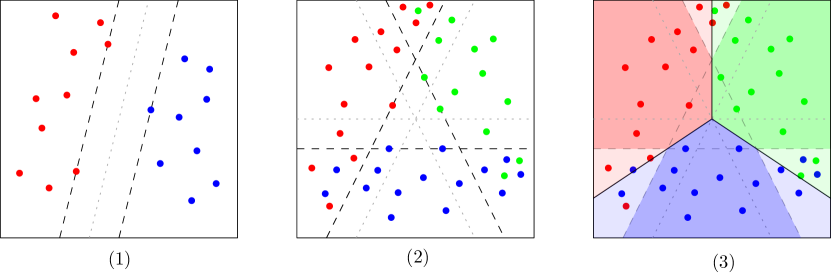
We describe how the half-spaces can be used to split into convex regions, each corresponding to an . The model can also be used to distinguish the regions of ambiguity. The subdivision of is most natural when .
We describe in Table 1 the complexity of computing these multi-class SVM. We compare directly with the complexity of computing a single SVM, to highlight the influence of the dimension.
(AvA) (1vA) (Simple TSVM) (TSVM) (randomized) (deterministic)
Statistical guarantees would be the same as those running a linear SVM with the parameters above. (Simple TSVM) and deterministic (TSVM) are equivalent to running a single SVM, while (TSVM), while randomized (TSVM) is equivalent to running binary SVMs.
Tverberg’s theorem is a challenging algorithmic problem [har2020journey]. One key difference between the problem addressed in this manuscript and the problem of finding Tverbreg partitions is that when training SVMs the labels are assigned before-hand. Tverberg’s theorem has also been applied to multi-class logistic regression [de2020stochastic].
Since the constructions are based on Sarkaria’s linear-algebraic technique, we can deduce several combinatorial properties of these multi-class SVMs. The model (simple TSVM) is invariant under orthogonal transformations, but not under translations. The model (TSVM) is invariant under any isometry of . To prove these properties, a closer look at Sarkaria’s method is needed, so the arguments presented here may be useful in the classic context of variations of Tverberg’s theorem.
We also discuss the existence and properties of support vectors. It is known that for any two separable sets , there exist such that and such that the largest-margin SVM induced by is the same as the largest-margin SVM induced by . For (TSVM) and (simple TSVM) a similar property holds. For any -tuples of sets , there is a -subset of that induces the same (TSVM). The same holds for (simple TSVM). In either case we call this -subset the support vectors of the multi-class SVM.
The manuscript is organized as follows. First, we present in Section 2 a new proof of a characterization of critical points in largest-margin SVMs. In Section 3 we describe the linear-algebraic tools needed for our constructions. In Section 4 we describe the models (TSVM) and (simple TSVM), and their main properties. In Section 5 we discuss the induced partitions of and finally in Section 6 we study how the model behaves when we apply orthogonal transformations to the sets of points.
2. Projection of support vectors.
Given two finite sets of points in that are linearly separable, let be a separating hyperplane at maximal distance from and . We denote by this distance, so
We say that a point in is a support vector if , and similarly for points in . We assign labels to the points so that the points of assigned positive and the points of are assigned negative.
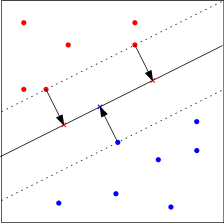
One interesting property about the projections of the support vectors is that the convex hulls of the projections onto the separating hyperplane of each side intersect, as in Fig. 2. This was proven independently by Veelaert and by Adams, Carr, and Farnell [Veelaert.2015, Adams2022]. One of the proofs involves the Karush–Kuhn–Tucker theorem and the other Householder transformations. We present an elementary proof.
Theorem 2.0.1.
Given a separable set of points in with two labels, the convex hulls of the projections of the negative and positive support vectors onto the induced largest margin SVM intersect.
Proof.
Let be the set of labeled points. Let be the separating hyperplane at maximum distance from the labeled sets, and let , be the positive and negative support vectors, respectively. Let be the distance of the support vectors to . This means that
Let be the orthogonal projection of onto , and be the orthogonal projections of onto . We assume that and look for a contradiction.
Since , there exists a co-dimension one affine subspace of that separates and . Notice that is a co-dimension two affine subspace of .
Let us project all the points into the two-dimensional subspace . We denote this projection by . In , is a line and is a point . Let be the orthogonal line to through .
The lines and split into four quadrants. Since , the points of and those of are separated by . They are also separated by by construction, so and are in opposite quadrants.
This means that we can rotate slightly around so that its distance to each point in and increases. If the angle of rotation is small enough, the distance of to the rest of the points in remains strictly larger than . This contradicts being the largest-margin SVM. ∎
3. Linear-algebraic tools
In this section, we introduce Sarkaria’s construction to tackle Tverberg-type problems. Suppose we are given sets in . We introduce , which are the vertices of a regular simplex in centered at the origin. We further assume that each is a unit vector. A crucial property of this -tuple is that its linear dependences are precisely the linear combinations in which all coefficients are equal. For each we associate to . Given we first append a coordinate to make it into a vector in , . Then, we take the tensor product with its corresponding , defining
In this manuscript we treat as the set of vectors and as the set of matrices interchangeably.
Finally, for , we define the set
The main difference with our approach and the one by Bárány and Onn is that for each point in we already know to which class it belongs, so it yields a unique point in the higher-dimensional space. When one wants to prove Tverberg’s theorem, we have to assign classes to unlabeled sets of points, so each point in is represented by a -tuple in .
The main reason why this transformation can be used to study Tverberg-type problems and why we can use it in the context of multi-class SVMs is the following lemma.
Lemma 3.0.1.
Let be positive integers. Let be finite sets of points in such that . Then, for defined as above, .
Proof.
Let and . We prove the contrapositive. Assume that the origin in is in the convex hull of . We want to show that the convex hulls of the sets intersect. Then, for each there exists a non-negative coefficient such that and
If we look at the linear dependences of in , we can see that if an only if . This carries through the tensor product and we have
This is an equality in . If we look at the last coordinate, we have Since the total sum of the coefficients was one, each of the sums above must be . If we look at the first coordinates and multiply each equation by , we have
and each of the terms above is a convex combination. This means that the convex hulls of the have non-empty intersection, . ∎
Therefore, the origin in can be separated from by a hyperplane. We can find this hyperplane with any existing algorithm for SVMs, which is the central point of this manuscript. If we have a hyperplane separating a set from the origin in , we want to obtain a set of half-spaces as described in the introduction.
In other words, we need to be able to map hyperplanes in into -tuples of hyperplanes in explicitly. This has been done recently [Sarkar:2020uk]. We describe the process below.
Let be the function that erases the last coordinate. For each let us think of as a matrix. For we define the function
where is considered as a product of matrices.
Lemma 3.0.2.
If , then .
Proof.
A simple computation shows that
The third equality follows since is a unit vector. ∎
For each , consider the -dimensional affine subspace . Given a half-space in , consider the half-spaces in defined by for .
Lemma 3.0.3.
Let be a closed half-space in . If then .
Proof.
As before, let’s consider as the set of matrices. Each closed half-space can be defined using a linear functional and a constant. Using the Frobenius product, we can express using a matrix and a constant such that
Since the origin is not contained in , we can assume that . Suppose on the contrary that there exists an so that and we look for a contradiction. In other words, for we have , so .
If we write each of the inequalities as varies and add them, we have
The last equality follows as . This is the contradiction we wanted. ∎
Now we have all the ingredients to define a multi-class SVM. Another important subspace for our computations is the following -dimensional space
This subspace has been used previously to prove some variations of Tverberg’s theorem with some coloring conditions added to the set [soberon2015equal]. Some particular translates of will also be useful. For we define
Notice that for each .
Lemma 3.0.4.
Let such that for each . The only point in is the barycenter of the set .
Proof.
Consider each as a matrix. Suppose that is a convex combination in . If we look at the last row of this linear combination we have . This means that , as we wanted. ∎
4. Construction and basic properties of multi-class SVM
We are now ready to formalize the multiclass SVMs described in the introduction. Given sets in whose convex hulls do not all overlap, we seek a family of half-spaces such that for each and so that the half-space do not all intersect. For the following definition we need the subspaces and their associated functions defined above.
Definition 1 (Simple TSVM).
Let be finite families of points in whose convex hulls do not intersect. We define the multi-class support vector machine (Simple TSVM) as a family of closed half-spaces obtained as follows. First, for each construct the point . Let be the collection of all points obtained this way. Find the closed half-space in that contains and whose distance from the origin is maximal. For the half-space is defined as .
The computation of (simple TSVM) consists of finding the distance from to the origin. We can also think of this as finding the largest-margin SVM in that separates the origin from , and then doubling the distance to the origin. The discussion in the previous section shows that this multi-class support vector machine satisfies the desired properties. For a soft-margin version, it suffices to compute in an SVM with one class equal to and the other equal to . If we denote by the complexity of an algorithm to compute an SVM with data points in and two classes of size and , then the complexity of computing (simple TSVM) is , where is the number of data points. Any other performance metrics we have for an SVM transfer to (simple TSVM) if we do the change of parameter as outlined above.
For the second type of multi-class SVM, we consider the following alternative definition. Recall that in the space of matrices we denoted by the subspace where the last row is equal to zero.
Definition 2 (TSVM).
Let be finite families of points in whose convex hulls do not intersect. We define the multi-class support vector machine (TSVM) as a family of closed half-spaces obtained as follows. First, for each construct the point . Let be the collection of all points obtained this way and consider . Compute the closest point of to the origin, and the closed half-space in that contains , whose boundary hyperplane contains , and whose distance from the origin is maximal. The half-spaces are defined as .
Even though this definition is more involved it has two big advantages. First, it is stable under translations of the sets of points. Second, in the case it is precisely a largest-margin SVM. We prove these properties in the next section. Just like SVM have critical points, any (TSVM) is fixed by a small set of points.
Theorem 4.0.1.
Let be finite sets in such that . We can find subsets such that induces the same (simple TSVM) as and such that
Proof.
We follow the construction in Definition 1. Since the closest point to the origin in must be in a face of the polytope . This face can have dimension at most . By Carathéodory’s theorem, we can choose a set of at most point in whose convex hull contains . The subsets of that induced this subset in satisfy the condition we wanted. ∎
Theorem 4.0.2.
Let be finite sets in such that . We can find subsets such that induces the same (TSVM) as and such that
Proof.
The proof is similar to the previous theorem. If we look for the minimal face of sustaining , it has dimension at most , so the same application of Carathéodory’s theorem yields the result. The only additional detail to check is that . This holds because for every choice , the baryceneter of the point is in . ∎
We denote the subsets obtained by Theorem 4.0.1 and Theorem 4.0.2 as the support vectors of a (simple TSVM) or (TSVM), respectively.
As mentioned above, to compute (Simple TSVM) we need to compute an SVM in a -dimensional space with points. A direct approach to compute (TSVM) would be to first find the vertices of and solve the induced SVM. We know is a linear subspace of co-dimension , so the vertices of should be the intersection of the -skeleton of with . Due to Lemma 3.0.4, this is a subset of the barycenters of -tuples with one element in each . Therefore, we can compute these barycenters and then compute an SVM in . This leads us to solve an SVM in a -dimensional space with points.
Theorem 4.0.2 shows that computing a TSVM can be treated as a linear programming type problem, as in the framework of Sharir and Welzl [Sharir:1992ih]. This is a randomized approach to problems which are combinatorially similar to linear programming problems, so that they can be solved in expected linear time in the input, which is a signficant reduction over brute-force approaches. This means that for fixed we can compute (TSVM) with a randomized algorithm in expected time linear in . We describe the process in Algorithm 1, before translating back to .
The key idea to compute this is to order the points randomly. At any point, we have computed (TSVM) for the first points and we keept track of the support vector of this TSVM. When including the -th point, if we don’t need to adjust the current halfspace generated by (TSVM), we keep goint. Otherwise, we adjust our guess for the support vectors and run the algorithm again for the first points. The computations of Sharir and Welzl bound the expected number of times we need to rerun this procedure, and end up with an expected running time linear on the input. For deeper explanations, we recommend references on linear-programming type algorithms and violator spaces [Gartner:2008bp, Amenta:2017ed].
The model (TSVM) generalizes largest-margin SVMs when . This is the main motivation to use the subspace in the computation. Let us prove that this is indeed the case.
Theorem 4.0.3.
For , the multiclass SVM (TSVM) gives the two support hyperplanes of the largest-margin SVM of and .
Proof.
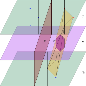
Notice that is the only case when for all values of . Additionally, each is a translate of . In this case we also have in . Therefore and . Let be the closest point of to the origin, and be the affine hyperplane in through from Definition 2. Let be the hyperplane through the origin of , parallel to , and let . Notice that is the distance between and . Since a translate of lies in , contains the support vectors in of in . The same holds for for the support vectors in , so contains the support vectors of in . This means that the (TSVM) induced by is an SVM at common distance from each side.
Similarly, given a separating hyperplane for at distance from each set, we can embed in and then reflect the embedding of with respect to the origin in so that it lies in . If we extend through the origin in , we have a hyperplane through the origin at distance from the convex hull of the embedding of in and in . The largest margin SVM must therefore coincide with the one induced by (TSVM). ∎
An illustration of the ideas behind this proof is shown in Fig. 3.
5. Subdivision of ambient space and potential classification errors
In each of Definition 1 and Definition 2 we use a half-space in that does not contain the origin to generate the corresponding half-space in .
In each case, we can introduce a half-space that is a translate of and whose boundary contains the origin. Notice that the half-spaces for have non-empty intersection but their interiors have an empty intersection. This is a direct consequence of Lemma 3.0.1 because contains the origin and the interior of does not.
As an illustration, for the two half-space from (TSVM) share their boundary, which is precisely the largest-margin SVM for .
Let and , where denotes the interior of for any . Now for we define the convex sets .
[\capbeside\thisfloatsetupcapbesideposition=right,top,capbesidewidth=8cm]figure[\FBwidth]
Intuitively, is the polytopal region not contained in the union of the . The set is an affine subspace inside . If , we the set is constructed by making a simplex in the orthogonal complement of and extending it in the directions of . The set is formed by taking all possible rays that start at and go in the direction of a point of in the boundary of . The case when is a simplex is perhaps the most illustrative one, since in this case is a point and we simply take the cones from towards each of the facets of . This case looks like Fig. 1 (3).
As mentioned before, the condition needed to generate (TSVM) or (simple TSVM) is that the convex hulls of the sets do not all overlap. If the convex hulls of fewer of these sets overalp, any model that subdivides into convex pieces is bound to miss-label some data. We minimize the misslabelings with our constructions.
6. Equivariance
In this section we describe how the multi-class SVMs we introduced interact with transformations of the set of points. It is clear that if we apply the same affine transformation to the sets of points and the half-spaces the containments are preserved, but we are interested to see if the algorithms to obtain behave as expected with these transformations.
Theorem 6.0.1.
Let be an orthogonal linear transformation of . Let be the (simple TSVM) induced by . Then is the (simple TSVM) induced by .
Proof.
First notice that can be extended to by acting on the first coordinates and leaving the last coordinate fixed. This is also an orthogonal transformation. We denote this transformation by , so . Finally, we denote by the transformation on that multiplies every column of a matrix by , so as a product of matrices.
This last transformation is also orthogonal. To see this, we first show that it preserves the dot product between vectors in and for any (possibly equal) and . We use a known factorization for the dot product of tensor products, as shown below.
Consider the union of an affine basis for each of . This set of vectors forms a basis of , and preserves the dot product between any two of these vectors. Therefore preserves the dot product in and is therefore orthogonal.
∎
Theorem 6.0.2.
Let be an orthogonal linear transformation of and be the (TSVM) induced by . Then is the (TSVM) induced by .
Proof.
We follow the ideas used in the proof of Theorem 6.0.1. We notice that fixes . Therefore, the restriction of to is an orthogonal transformation. This means that for any half-space in , we have . Again, if is the half-space in that induces our (TSVM), we have that is the half-space for the new set of points.
Now, if we consider the (TSVM) induced by , we have to find the half-space in farthest from the origin that contains . Clearly, is the farthest half-space from the origin that contains . For , we also have . ∎
Theorem 6.0.3.
Let be a vector in . Let be the set of support vectors of the (TSVM) induced by . Then is the set of support vectors of the (TSVM) induced by .
Proof.
To find the (TSVM) incuded by we need to compute . Notice that this set is invariant under translations of . This is because for any points the barycenter of is the same as the barycenter of . Since does not change, the set of support vectors remains the same. ∎
7. Acknowledgments
The author thanks Henry Adams for helpful comments.