Clique Is Hard on Average for Sherali-Adams
with Bounded
Coefficients††thanks: This is the full-length version of a paper
with the
title “Clique Is Hard on Average for Unary Sherali-Adams”
that appeared in the Proceedings of the 64th Annual IEEE
Symposium on Foundations of Computer Science (FOCS ’23).
Abstract
We prove that Sherali-Adams with polynomially bounded coefficients requires proofs of size to rule out the existence of an -clique in Erdős-Rényi random graphs whose maximum clique is of size . This lower bound is tight up to the multiplicative constant in the exponent. We obtain this result by introducing a technique inspired by pseudo-calibration which may be of independent interest. The technique involves defining a measure on monomials that precisely captures the contribution of a monomial to a refutation. This measure intuitively captures progress and should have further applications in proof complexity.
1 Introduction
The problem of identifying a maximum clique in a given graph, that is, finding a fully connected subgraph of maximum size, is one of the fundamental problems of theoretical computer science. Already mentioned by Cook [Coo71] in his seminal paper introducing the theory of NP-complete problems, it was one of the first combinatorial problems proven NP-hard by Karp [Kar72]. Building on the PCP theorem this result was later strengthened to even rule out polynomial time algorithms that approximate the maximum clique size within a factor of [Hås99, Zuc07], unless .
A related problem is -clique: given an -vertex graph, determine whether it contains a clique of size . This problem can be solved in time by iterating over all subsets of vertices of size and checking whether one of them is a clique. This naïve algorithm is essentially the fastest known; a clever use of fast matrix multiplication [NP85] allows a slight improvement upon the constant in the exponent but no algorithms with a sublinear dependence on in the exponent are known.
If we only assume , it is unknown whether there are faster algorithms for -clique. However, improving upon the linear dependence on in the exponent would disprove the exponential time hypothesis [CHKX04] and getting rid of the dependence on altogether would imply that the class of fixed parameter tractable problems collapses to [DF95]. Hence, if one is willing to make the strong assumption that the exponential time hypothesis holds, then the naïve algorithm has essentially optimal running time in the worst-case.
Besides studying -clique in the worst-case, one may consider it in the average-case setting. Suppose the given graph is an Erdős-Rényi graph with edge probability around the threshold of containing a -clique. Does -clique require time on such graphs? Or, even less ambitiously, is there an algorithm running in time that decides the -clique problem on such graphs? It is unlikely that the hardness of such average-case questions can be based on worst-case hardness assumptions such as or the exponential time hypothesis [BT06]. They are, in fact, being used as hardness assumptions themselves: the planted clique conjecture states that -clique requires time on Erdős-Rényi graphs with edge probability .
In order to obtain unconditional lower bounds – that do not rely on hardness assumptions – for such average-case questions, we focus on limited models of computation. This approach has turned out to be quite fruitful and several results of this form have emerged over the past few decades. For Boolean circuits, Rossman [Ros08, Ros10] proved two remarkable results: he showed that monotone circuits, i.e., circuits consisting of and gates only, as well as circuits of constant depth require size to refute the existence of a -clique in the average-case setting.
Instead of studying circuits, it is also possible to approach this problem through the lens of proof complexity. Very broadly, proof complexity studies certificates of unsatisfiability of propositional formulas. As we cannot argue about certificates of unsatisfiability in general we consider certificates of a certain form, or in terms of proof complexity, refutations in a given proof system. For instance, if we prove that any certificate in a proof system that witnesses that a given -vertex graph contains no -clique requires length on average, then we immediately obtain average-case running time lower bounds for any algorithm whose trace can be interpreted as a proof in the system . It is often the case that state-of-the-art algorithms can be captured by seemingly simple proof systems, as was shown to be the case for clique algorithms [ABdR+21].
It is often the case that weak proof systems are sensitive to the precise encoding of combinatorial principles. The -clique formula is no exception: it is somewhat straightforward to prove almost optimal resolution size lower bounds for the less usual binary encoding of the -clique formula [LPRT17] and these lower bounds can even be extended to an lower bound for the Res() proof system for constant [DGGM20]. For the more natural unary encoding not much is known. There are essentially optimal average-case size lower bounds for regular resolution [ABdR+21, Pan21a] and tree-like resolution [BGLR12, Lau18]. For resolution, there are two average-case lower bounds that hold in different regimes: for , Beame et al. [BIS07] proved an average-case size lower bound and for , Pang [Pan21a] proved a lower bound. It is a long standing open problem, mentioned, e.g., in [BGLR12], to prove an unconditional resolution size lower bound for the unary encoding – even in the worst case.
Little is known about the average-case hardness of the -clique formula in the semi-algebraic setting. There are optimal degree lower bounds for for the Sum-of-Squares proof system [MPW15, BHK+19, Pan21b], but there are no non-trivial lower bounds on size. For Nullstellensatz, however, if restricted to not use dual variables, then size lower bounds follow by a simple syntactic argument [Mar08]. Prior to our work no other size lower bounds were known for algebraic or semi-algebraic proof systems.
1.1 Our Result
In this work we establish that Sherali-Adams [SA94, DM13] with polynomially bounded coefficients requires size to refute the -clique formula on random graphs whose maximum clique size is of size . Qualitatively this establishes the planted clique conjecture for Sherali-Adams with polynomially bounded coefficients. This is the first size lower bound on the clique formula for a semi-algebraic proof system.
Theorem 1.1 (Informal).
For all integers and , if is an Erdős-Rényi random graph, then it holds asymptotically almost surely that Sherali-Adams with polynomially bounded coefficients requires size at least to refute the claim that contains a clique of size , for any .
Note that Sherali-Adams with polynomially bounded coefficients is stronger than unary Sherali-Adams and is incomparable to resolution [GHJ+22]. Our result further applies to the SubCubeSums proof system [FMSV23] as our proof strategy gives a lower bound on the sum of the magnitude of the coefficients of a Sherali-Adams refutation, ignoring Boolean axioms.
Let us stress that the size lower bound holds regardless of the degree of the refutation. This is a somewhat unique feature of our technique – all other lower bound strategies for Sherali-Adams and Sum-of-Squares are tailored to proving degree lower bounds, which, if strong enough, imply size lower bounds by the size-degree relation [AH19]. Since the clique formula has refutations of degree we cannot expect to obtain size lower bounds through this connection for . We therefore introduce a new technique, inspired by pseudo-calibration [BHK+19], that is more refined – for any monomial , of arbitrary degree, we determine a lower bound on the size of the smallest bounded-coefficient Sherali-Adams derivation of .
1.2 Organization
The rest of this paper is organized as follows. In Section 2 we introduce some basic terminology to then outline our proof strategy in Section 3 where we also attempt to convey some intuition. With the motivation at hand from Section 3 we then go on to define the central combinatorial concept of a core of a graph in Section 4 and a notion of pseudorandomness in Section 5. We proceed in Section 6 to prove the main theorem for any graph satisfying our notion of pseudorandomness, but postpone the proof of one of the main lemmas to Section 7. Finally, in Section 8, we show that a random graph satisfies our pseudorandomness property and conclude with some open problems in Section 9.
2 Preliminaries
Natural logarithms (base ) are denoted by , whereas base logarithms are denoted by . For integers we introduce the shorthand and sometimes identify singletons with the element . Let denote the set of subsets of of size and, for a given a random variable and an event , we denote by the indicator random variable that is if holds and otherwise.
2.1 Semantic Sherali-Adams
Let be a polynomial system of equations over Boolean variables and their twin variables . Denote by
| (2.1) |
the corresponding Boolean axioms and negation axioms and let denote the ideal generated by , that is, consists of all polynomials of the form where the are arbitrary polynomials and . For an ideal and polynomials and we write if .
A semantic Sherali-Adams refutation of is a sequence of polynomials such that is of the form
| (2.2) |
and it holds that
| (2.3) |
The size of a refutation , denoted by , is the sum of the size of the binary encodings of the non-zero coefficients on the left hand side of (2.3) when all polynomials are expanded as a sum of monomials (without cancellations), while the coefficient size of is the sum of the magnitudes of the coefficients of the aforementioned monomials.
We note that this definition differs from that of the usual Sherali-Adams proof system [SA94, DM13] where Boolean axioms and negation axioms are written out explicitly and the size is measured taking also these axioms into account. We are not the first to disregard the size contribution of these axioms: most size lower bounds for Sherali-Adams also apply in this setting. The question of whether these two size measures are polynomially related was raised explicitly in [FHR+24], where the above system is referred to as succinct Sherali-Adams, and remains open.
To verify that semantic Sherali-Adams is a Cook-Reckhow proof system, we need to check that a semantic Sherali-Adams refutation is verifiable in time polynomial in the size of the refutation. This was originally shown in [FHR+24], but we provide a simpler and more direct proof of this fact.
Proposition 2.1.
Let be a polynomial system of equations over Boolean variables and their twin variables. A semantic Sherali-Adams refutation of can be verified in time .
Proof.
Denote the coefficient of a monomial in a polynomial by . Further, given a monomial , let be the vector of length , indexed by assignments , that corresponds to the truth table of : the entry with index is if the monomial evaluates to under and otherwise. We denote the all-ones vector by , and the all-zero vector by .
With this notation at hand we may equivalently define a semantic Sherali-Adams refutation of as a sequence of rational vectors indexed by multilinear monomials with and
| (2.4) |
View the left hand side as a vector indexed by assignments . Since the vector is rational, we have that is the -vector if and only if the inner product is , that is, . This can be efficiently checked by expanding the inner product
| (2.5) | ||||
Observe that in the above expression all the inner products can be efficiently computed. Hence checking whether is indeed a valid semantic Sherali-Adams refutation boils down to verifying that the above sum of bounded rationals is equal to . ∎
As the distinction between semantic Sherali-Adams and Sherali-Adams is not essential for what follows, we refer to semantic Sherali-Adams simply as Sherali-Adams going forward. A Sherali-Adams refutation of is a Sherali-Adams refutation with -bounded-coefficients if the magnitude of all coefficients is bounded by and we call a Sherali-Adams refutation with -bounded-coefficients if for some constant it holds that is a Sherali-Adams refutation with -bounded-coefficients. Let us record the following observation.
Proposition 2.2.
If Sherali-Adams requires coefficient size to refute , then Sherali-Adams with -bounded-coefficients requires size to refute .
Proof.
As every coefficient in an -bounded-coefficient refutation is bounded by , there need to be at least monomials with a non-zero coefficient. ∎
Unary Sherali-Adams is a subsystem of Sherali-Adams where all coefficients of monomials are either or and the right-hand-side of Equation 2.3 is any negative integer
| (2.6) |
where is again a non-negative sum of monomials.
Proposition 2.3.
If Sherali-Adams requires coefficient size to refute , then unary Sherali-Adams requires size at least to refute .
Proof.
We can transform any unary Sherali-Adams refutation of size , summing to an integer , to a Sherali-Adams refutation of coefficient size at most by dividing the left hand side by . ∎
2.2 Graph Theory
Before defining the -clique formula, we introduce some terminology and notation that we use throughout the paper.
Unless stated otherwise, denotes a -partite graph with partitions of size each. We call a partition a block and, for , denote by the vertices in blocks in , that is, . For disjoint sets we let a tuple be a sequence of vertices satisfying for all . All tuples we consider are defined with respect to the partition , though, at times, may only be defined over a subset of the blocks, that is, not all tuples are of size . For a tuple and a set we denote the projection of onto by . An -tuple is a tuple of size and sometimes it is convenient for us to think of a tuple as a set of vertices. We take the liberty to interchangeably identify a tuple as a sequence as well as a set and hope that this causes no confusion.
A set of tuples is a rectangle if for some the set can be written as the Cartesian product of sets for , i.e., ; in other words, contains all tuples satisfying for all . Rectangles, unless explicitly stated, consist of -tuples only, that is, . Given a rectangle and a set we let be the projection of onto the blocks in : if , then and, in particular, we have for .
While always denotes a large graph, the graphs and denote small graphs: throughout the paper and are graphs on labeled vertices. Usually these graphs have a small vertex cover and graphs denoted by furthermore have many isolated vertices. For a graph we denote the minimum vertex cover by and sometimes refer to as a pattern graph, whereas is usually a core graph (see Section 4). We denote by the set of graphs on labeled vertices and for a parameter let be the family of graphs with a minimum vertex cover of size at most , that is, all graphs satisfy .
We record here two simple lemmas about graphs that will come in handy throughout the paper.
Lemma 2.4.
There are at most graphs over vertices with a vertex cover of size and .
Proof.
We first choose the vertices from the vertices that form the vertex cover. Then, from the remaining vertices, we choose vertices that may be incident to an edge. We can add edges that are incident to the vertex cover and the other vertices and thus get that there are at most
| (2.7) |
many such graphs. ∎
Recall that a maximal matching of is a matching that cannot be extended in .
Proposition 2.5.
Any maximal matching in a graph is of size at least .
Proof.
Since is maximal, all edges of are incident to . Thus the set is a vertex cover of . ∎
The distribution of random graphs we consider in this paper is a -partite version of the Erdős-Rényi distribution. For a fixed set of vertices and a real number , the Erdős-Rényi distribution is the distribution of random graphs on vertex set where every potential edge , for vertices , is sampled independently with probability . As was done in [BIS07, ABdR+21], we work with the block model, which is defined as follows. Given blocks of size and a real number , we denote by the distribution over graphs on the vertex set defined by sampling each edge independently with probability if and are in distinct blocks. We sometimes refer to such pairs of vertices as potential edges. Edges within the same block are never included and hence is a distribution over -partite graphs.
2.3 Clique Formula
Below we present an encoding of the -clique formula on -partite graphs as a system of polynomial equations.
Given a -partite graph with blocks of size we define the -clique formula over stating that has a -clique (with one vertex per block) as follows. The formula is defined over variables: each vertex is associated with two variables and . The intended meaning is that is if is in the identified -clique and otherwise, and . Since we define the Sherali-Adams proof system (see Section 2.1) to operate modulo the ideal generated by the Boolean axioms and the negation axioms , we do not need to explicitly include such axioms in the formula.
For each block we introduce the block axiom stating that precisely one vertex from each block is chosen and for each pair of vertices in distinct blocks we introduce the edge axiom that ensures that non-neighbors are not simultaneously selected. We note that we could also include edge axioms for pairs of vertices in the same block but we choose not to since these are easily derivable from the block axioms.
It should be evident that this formula is satisfiable modulo the Boolean and the negation axioms if and only if there is a -tuple such that the vertex induced subgraph is a clique.
We make two remarks about this choice of encoding. The first is that our lower bound strategy is completely agnostic to the encoding of the block axioms. We could equally well have considered the polynomial translation of the CNF encoding, or the binary encoding, or any encoding of the constraints that one vertex of each block should be chosen to be part of the clique.
The second remark is that, as argued in Beame, Impagliazzo and Sabharwal [BIS07], the reason for choosing to define the formula over -partite graphs is that proving a lower bound for this encoding implies a lower bound for other natural encodings. In particular, if we consider the -clique formula defined over a (not necessarily -partite) graph on vertices, as the formula containing the axiom and edge axioms for each pair of vertices , then for any equal-sized -partition it holds that a lower bound for the -clique formula on with this partition implies the same lower bound for the non--partite formula.
Proposition 2.6 ([BIS07]).
Let be integer and let be a graph on vertices. Then the minimum Sherali-Adams coefficient size to refute the -clique formula over is bounded from below by the coefficient size required to refute the -clique formula defined with respect to any equal-sized -partition of .
This proposition was proven in [BIS07] for resolution size, and it is straightforward to see that it holds for Sherali-Adams coefficient size. Indeed, it is enough to observe that the non--partite -clique formula can be easily derived from the -partite -clique formula.
3 Main Theorem and Proof Overview
The main result of this paper is a tight, up to constants in the exponent, Sherali-Adams coefficient size lower bound for -clique formulas over Erdős-Rényi random graphs.
Theorem 3.1 (Main theorem).
Let and be functions of such that and . If , then asymptotically almost surely Sherali-Adams requires coefficient size to refute the -clique formula over .
Note that Theorem 1.1 follows directly from Theorem 3.1 along with Propositions 2.6 and 2.2, where we assume that the coefficient size is bounded by a polynomial where is a constant independent of . The main result of the conference version of this paper [DRPR23] follows from Theorem 3.1 and Propositions 2.6 and 2.3.
In the rest of this section we outline our proof strategy. We intend to come up with a so-called pseudo-measure which lower bounds the coefficient size of a Sherali-Adams refutation. Before we get ahead of ourselves let us define what a pseudo-measure is.
Definition 3.2 (Pseudo-measure).
Let and be a set of polynomials over the polynomial ring . A linear function , mapping polynomials to reals, is a -pseudo-measure for if for all monomials and all polynomials it holds that
-
1.
,
-
2.
, and
-
3.
.
A concept related to the notion of a pseudo-measure has previously appeared in [PZ22] for the Nullstellensatz proof system over the reals. We also note that in a recent work Hubáček, Khaniki and Thapen [HKT24] defined a similar notion for Sherali-Adams with bounded degree. We have the following simple proposition.
Proposition 3.3.
There is a -pseudo-measure for if and only if any Sherali-Adams refutation of requires coefficient size .
Proof.
Given a monomial , let be the vector of length , indexed by assignments , that corresponds to the truth table of , that is, on index the vector is if the monomial evaluates to on assignment and otherwise. We denote the all-ones vector by .
Let be a polynomial system of equations over Boolean variables and their twin variables . We denote the coefficient of a monomial in a polynomial by . We may write a linear program that searches for a Sherali-Adams refutation of of minimum coefficient size as
| (3.1) |
We appeal to duality to obtain the following dual program to the above. Denote by the vector of dual variables of dimension and introduce for a monomial the shorthand and for a polynomial let . The dual to the above linear program may be expressed as
| (3.2) |
Thus the notion of a pseudo-measure for is indeed the dual object of a Sherali-Adams refutation of with small coefficient size. By appealing to strong duality and normalizing by the claim follows. ∎
3.1 Our Pseudo-Measure
In what follows we define our pseudo-measure for the -clique formula. We may think of as a progress measure: it assigns to each monomial a real value which can be thought of as the contribution of this monomial towards the refutation of the -clique formula. Thus, intuitively, we would like to associate each monomial with the fraction of potentially satisfying assignments that it rules out. In order to define this a bit more formally, let us introduce the set of potentially satisfying assignments.
We say that an assignment is potentially satisfying for the -clique formula if there is a graph such that the -clique formula defined over is satisfied by . This set of assignments can be easily characterized: if we associate each -tuple with the assignment that sets all variables to if and to otherwise, then the set of potentially satisfying assignments of the -clique formula is
| (3.3) |
We say that a monomial rules out an assignment if . As there is a one-to-one correspondence between potentially satisfying assignments and tuples, it is convenient to think of the tuples that a monomial rules out. We thus associate each monomial with the set
| (3.4) |
of ruled out -tuples. Note that is the set of all tuples, that is, and the set associated with an edge axiom consists of all -tuples that contain the vertices and .
More generally, it is not too hard to see that the set of ruled out tuples of a monomial is a rectangle and that for each rectangle there is at least one monomial such that is the set of tuples ruled out by . We thus often discuss rectangles and it is implicitly understood that if a statement holds for all rectangles, then it also holds for all monomials. Finally, observe that if a monomial satisfies , then .
For intuition we will now discuss two naïve, and fatally flawed, attempts to define a pseudo-measure. For our first attempt, we simply associate each monomial with the fraction of ruled out tuples, that is we map a monomial to
| (3.5) |
This measure maps the monomial to and is clearly non-negative and hence satisfies Items 1 and 3 of Definition 3.2 for any . Furthermore, again for any , it satisfies Item 2 of Definition 3.2 for the block axioms. Only the edge axioms cause trouble: the rectangle associated with the edge axiom is a fraction of all tuples. As such, according to Proposition 3.3, this pseudo-measure may only gives us an coefficient size lower bound—not quite what we are after.
We may try to remedy this by not associating a monomial with all tuples in but rather only with a subset of that depends on the graph . One very naïve attempt would be to associate with the number of -cliques that it rules out, that is, we may associate a monomial with the normalized measure
| (3.6) |
This definition, at least in expectation over , satisfies all properties of a pseudo-measure: the monomial is mapped to , the axioms are all mapped to and the measure is non-negative.
The obvious problem is that all graphs we consider do not contain a -clique and hence everything (including the monomial ) is mapped to . Put differently, the main problem is that the random variable over has too large variance. We reduce this variance as pioneered by Barak et al. [BHK+19]: we expand Equation 3.6 in the Fourier basis and truncate the resulting expression. A careful choice of the truncation, along with some significant effort, allows us to argue that, on the one hand, the measure associated with is large (i.e., the variance is reduced) while, on the other hand, the measure associated with edge axioms is still tightly concentrated around and that the measure is essentially non-negative (i.e., the variance did not increase significantly). This measure thus constitutes a valid pseudo-measure as defined in Definition 3.2 up to normalization. In order to state the precise definition of our pseudo-measure we need some notation.
If denotes the probability that a potential edge is present in the graph, then the character is defined by
| (3.7) |
and for a set of potential edges we let . It is convenient for us to work with the above (non-standard) basis as it allows us to easily cancel characters in case an edge is missing. Observe that for this is the usual Fourier basis. First time readers are advised to keep this case in mind for the remainder of the article. Let us record some useful facts.
Proposition 3.4.
Let , let and . For any potential edge , sampled with probability , it holds that and . In particular, for , we have . A useful bound is . Finally, observe that for any tuple we have that is if is a clique and otherwise.
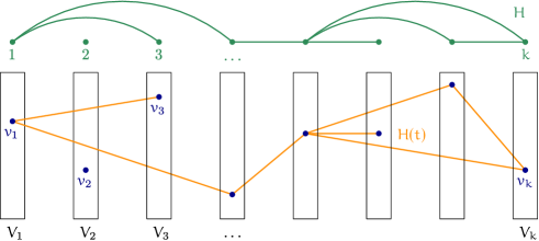
To concisely state our pseudo-measure we need some further notation. We consider sums of tuples and want to treat edge sets that are equal up to the mapping onto a -tuple as the same. More precisely, if we have two -tuples and edge sets and such that if and only if , then we want to identify and as the same edge set. To this end we consider pattern graphs (similar to the shape graphs in the terminology of [BHK+19]) over the vertex set . For a tuple and a pattern graph we let be the edge set that contains the edge if and only if the edge is present in . See Figure 1 for an illustration.
With this notation at hand we define our pseudo-measure as
| (3.8) |
where the second sum is over all graphs over vertices with vertex cover at most , and is a small constant times the maximum clique size of .
Observe that Boolean axioms, the negation axioms and the block axioms multiplied by an arbitrary monomial are all mapped to by . Hence it remains to prove that the measure maps the constant monomial to a large value, that is small on subrectangles of edge axioms, i.e., any edge axiom multiplied by a monomial is mapped to a small value, and that all monomials are mapped to an approximately non-negative value.
By inspecting the second moment of it is not too hard to see that there is quite a bit of freedom on how to choose the truncation in the definition of while maintaining the property that asymptotically almost surely. However, ensuring that the edge axioms are associated with small measure is more delicate. Here we heavily rely on our choice to truncate according to the minimum vertex cover. More specifically we rely on two crucial properties of graphs satisfying : firstly, we use the fact that such graphs contain a matching of size (see Proposition 2.5) and, secondly, that the family of these graphs satisfies a monotonicity property which leads to a useful partition of this family. For more details about this partition we refer to Section 4. Let us mention that it is conceivable that one could increase the bound on for which our results hold by truncating according to the size of the maximum matching. As we do not know how to define the above mentioned partition with respect to the maximum matching we truncate according to the minimum vertex cover.
In the following sections we try to present some intuition as to why is a pseudo-measure up to normalization, that is, why it satisfies Definition 3.2 where Item 1 is relaxed to approximately . In Section 3.2 we verify that sampled from asymptotically almost surely satisfies . As mentioned, this follows by a straightforward second moment argument. In Section 3.3 we outline why any subrectangle of an edge axiom satisfies . This proof motivates the definitions in Sections 4 and 5. Finally, in Section 3.4, we provide some high-level overview of how to prove that any rectangle is mapped to an approximately non-negative value, that is, it holds that . This is the most technically challenging part of the paper.
3.2 Expected Behavior of Our Pseudo-Measure
The measure of any rectangle satisfies
| (3.9) |
In particular, as , it holds that . In what follows we show that, for , the measure is somewhat concentrated around the expected value. The concentration, though, is far from enough to perform a union bound over all rectangles to argue that the measure behaves as expected on all rectangles simultaneously.
We show that the measure concentrates by an application of Chebyshev’s inequality. To this end we analyze the second moment: for we have
| (3.10) | ||||
| (3.11) | ||||
| (3.12) | ||||
| (3.13) | ||||
| (3.14) |
A careful application of Lemma 2.4 allows us to bound the number of pattern graphs we sum over in (3.14) to conclude that , as long as and are small. By virtue of Chebyshev’s inequality we then conclude that asymptotically almost surely.
A natural attempt to prove that the measure is mostly non-negative is to analyze higher moments in the hope that these are closely concentrated around the (positive) expected value. The fundamental difficulty in analyzing the pseudo-measure is that we have to analyze exponentially many rectangles simultaneously. Since there is such a large number of rectangles, for each input graph , there will be some rectangles where the value of differs considerably from the expected value.
For example, the measure on a rectangle with only a few vertices in some block heavily depends on the behavior of the edges incident to the vertices in . Hence, if is small enough, we expect large deviations from the expected value. A slightly simplified, though more concrete, example of this phenomenon goes as follows: let and , let be the rectangle that consists of all tuples that contain as well as , and let be the graph with the single edge . In this setting the sum heavily depends on whether the edge is present in : if the edge is present, then the sum is equal to and, if the edge is not present, then it is equal to . This indicates that on some rectangles the measure heavily depends on a few edges and we can thus not hope to naïvely prove concentration of the measure over all rectangles.
This slightly simplified example can be generalized to show that for a fixed there is always a small number of rectangles where the value contributed by is much larger than expected. Part of the technical challenge of the proof is to identify these bad rectangles and to handle them separately.
3.3 Edge Axioms Should Have Small Measure
We now explain the main ideas for bounding the magnitude of the measure of edge axioms. Recall that all other axioms are mapped to by and we are thus just left to show that the value of the edge axioms is closely concentrated around .
For every pair of vertices in distinct blocks we have an edge axiom stating that at least one of and are set to . Let be a subrectangle of . Note that for every such rectangle there is a monomial such that and hence these are the correct rectangles to consider if we want to prove Item 2 of Definition 3.2. In other words, if we manage to show for all such that , then it follows that for all monomials it holds that , as needed.
We first show that for a fixed pair of vertices , with good probability, all such subrectangles have small absolute measure. By a union bound over all missing edges we then conclude that all subrectangles of an edge axiom satisfy . Let us fix an edge .
If is empty, then there is nothing to prove as is trivially . Hence we may assume that is non-empty, that is, has at least one vertex per block and hence each tuple in contains both and . Let such that and . For we may write
| (3.15) | ||||
| (3.16) | ||||
| (3.17) |
where the last equality follows from the fact that every tuple contains and and thus, if , then as .
The naïve approach to bounding is to try to bound the magnitude of for each separately and to then multiply this bound by the number of graphs we sum over. Recall from Lemma 2.4 that there are about graphs with a minimum vertex cover of size . As the magnitude of typically has value , for large rectangles , even with the optimal bound , we can only show a bound of
| (3.18) |
Note that for much larger than both and the bound is at best . We require a bound of the form , which is much smaller than .
Instead of bounding the magnitude of for each separately, we partition the relevant set of graphs into different families and proceed to bound the magnitude of for each such family . More precisely, we have families of graphs indexed by graphs with at most non-isolated vertices of the form
| (3.19) |
that partition the set of graphs satisfying and . Using these families we can bound the magnitude of by
| (3.20) | ||||
| (3.21) | ||||
| (3.22) |
Observe that the innermost sum is, up to normalization, the indicator function of whether the edge set is present in . In fact the innermost sum, with the appropriate definition of , is simply a statement about the common neighborhood sizes of different subsets of in . We will need to argue that for random graphs, with high probability, all such sets behave as expected and the innermost sums are therefore bounded.
Furthermore, since each graph has at most with incident edges, there are fewer such graphs: according to Lemma 2.4 at most . Since and , for some small constant , it holds that there are at most many such graphs . Thus, an upper bound of on the absolute value of two innermost sums in Equation 3.22 can now be used to obtain the claimed bound . This completes the proof sketch for bounding the measure on edge axioms.
In Section 4 we formally define these core graphs and the families . In Section 5 we introduce the pseudorandomness property of graphs we rely on in order to bound the two innermost sums in Equation 3.22. In Section 6.1 we formally prove that the measure on subrectangles of axioms is bounded in absolute value and lastly, in Section 8, we verify that random graphs indeed satisfy the necessary pseudorandomness properties.
3.4 Rectangles Should Be Approximately Non-Negative
To show that all rectangles have essentially non-negative measure, the main idea is to decompose into a collection of rectangles satisfying the following properties.
-
1.
The collection is small, that is, .
-
2.
Each rectangle is either
-
(a)
very small: and hence is negligible,
-
(b)
a subrectangle of an axiom and thus, as argued in Section 3.3, is bounded, or
-
(c)
all common neighborhoods in are of expected size and therefore
(3.23)
-
(a)
In other words, contains some rectangles that have negligible measure and a collection of larger rectangles on which the measure behaves as expected. As the latter rectangles have strictly positive measure we may conclude that our pseudo-measure is essentially non-negative on all rectangles.
We bound the measure on small rectangles by summing the maximum possible magnitude of any character appearing in the definition of our pseudo measure.
Lemma 3.5.
Any rectangle satisfies .
Proof.
We bound by counting the number of pattern graphs we sum over multiplied by the maximum magnitude of each such character. We have that
| (3.24) | ||||
| (3.25) | ||||
| (3.26) |
as claimed. ∎
We implement the above proof outline in Section 6.2. Proving that our pseudo-measure concentrates around a positive value on rectangles as described in Item 2c is the most delicate part of our proof. In fact, the above proof outline is somewhat inaccurate in that the value the pseudo-expectation concentrates around is not simply but further depends on the number of small blocks in the rectangle . We refer to Definition 6.6 for the precise definition of these rectangles and to 6.7 for the claimed concentration inequality. Section 7 is dedicated to the proof of 6.7.
4 Cores
In this section we introduce the notion of a core of a pattern graph, which will be used extensively throughout the rest of the paper. Our notion of a core seems to be loosely connected to the notion of a vertex cover kernel as used in parameterized complexity (see, e.g., the survey by Fellows et al. [FJK+18]).
4.1 Cores and Boundaries
Recall that when bounding the measure of subrectangles of axioms , we were left with sums over graphs such that and (see Equation 3.17). Such graphs motivate the following definition of sets of graphs in the boundary of an edge.
Definition 4.1 (Boundary).
Let , be a graph and be an edge. The graph is in the -boundary, denoted by , if and only if and . Furthermore, we say that is in the -boundary if and only if is in an -boundary for some .
As mentioned in the proof sketch bounding the edge axioms, we cannot bound each in the -boundary separately (there are too many pattern graphs ) so we partition such graphs according to cores as explained below.
Definition 4.2 (Core).
A vertex induced subgraph of is a core if any minimum vertex cover of is also a vertex cover of .
Ultimately we are interested in cores that are induced by small vertex sets. It turns out that, in general, we cannot hope for cores of a graph that are induced by fewer than many vertices: as the graph that consists of vertex disjoint paths of length has only a single core , the best we can hope for are cores of size .
The notions of cores and -boundaries interact nicely in the following sense.
Proposition 4.3.
A core of a graph is in the -boundary if and only if is.
Proof.
Let be a core of . We first argue that if a core of the graph is in the -boundary, then so is . Indeed, by definition it holds that . Moreover, being in the -boundary implies that the minimum vertex cover of has size , and therefore the minimum vertex cover of must also be since is a subgraph of .
It remains to argue that if is in the -boundary, then so is the core . By definition of core, . Suppose, for the sake of contradiction, that is not in the -boundary and thus . Let be a minimum-sized vertex cover of . Since , it holds that is also a minimum-sized vertex cover of and thus, by definition of core, is also a vertex cover of . But this contradicts the assumption that is in the -boundary since also covers the edge and hence is a vertex cover of size of . ∎
Recall that is the set of graphs on labeled vertices. We consider a map from to small cores that satisfies certain properties as described below.
Theorem 4.4.
There is a map that maps graphs to a core of with the following properties. For every graph in the image of we have that and that there exists an edge set such that if and only if for .
We prove Theorem 4.4 in Section 4.2 below. From now on we only consider the cores given by the map as in Theorem 4.4. With a slight abuse of nomenclature we say that is the core of . Note that for a graph in the image of we have that , as introduced in Section 3.3.
4.2 Proof of Theorem 4.4
We first explain how to construct a map and then prove that it satisfies the required properties. In order to construct the mapping we require an order on subsets of vertices of : consider every subset of vertices as a sequence of vertices sorted in ascending order and say that a set is lexicographically smaller than a set if the ascending sequence of is lexicographically smaller than the sequence of , that is, for compare with : if (respectively ), then is lexicographically smaller (respectively larger) than ; if continue with ; if the prefix of length is equal, then is lexicographically smaller (larger) than if (respectively ).
Equivalently is lexicographically smaller than if the smallest element in the symmetric difference of and is contained in . From this alternate definition we immediately obtain the following property of the order.
Fact 4.5.
Let and be sets such that is lexicographically smaller than and . Then, for any element , the set is lexicographically smaller than .
We extend this notion in the natural manner to vertex covers and say that a minimum vertex cover is the lexicographically first minimum vertex cover of if is the lexicographically smallest minimum vertex cover of .
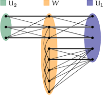
The map is constructed as follows (see Algorithm 1 for an algorithmic description). Given a graph with lexicographically first minimum vertex cover define the following two sets and of vertices. Let be the lexicographically first maximal (with respect to set inclusion) set of vertices with a matching from to that covers all of , that is, and . Similarly let be the lexicographically first maximal set of vertices with a matching from to of size . The core of is defined to be . An illustration is provided in Figure 2.
Let us record some simple observations
Claim 4.6.
For , and matchings defined as above, it holds that
-
1.
,
-
2.
any edge is incident to , and
-
3.
any edge is incident to .
Proof.
Since , it follows that . To argue that this map satisfies the other required properties, we first prove that the size of the minimum vertex cover of is the same as that of . Clearly so it remains to prove the opposite inequality.
Lemma 4.7.
For , and defined as above, it holds that .
Proof.
Let be the matching from to that covers and let be the vertices in that are not matched by , that is, . Towards contradiction suppose that the graph has a vertex cover of size .
By 4.6, Item 2, the only edges in which do not appear in the graph are edges between a vertex in and a vertex outside of .
Let be a vertex cover of of size that maximizes . If is a vertex cover of we have reached a contradiction. Otherwise, there exists a vertex that is not contained in and an edge for .
We now want to argue that either we can construct a vertex cover of of size that contradicts the fact that maximized , or we can construct a strict superset of with a matching to , contradicting the maximality of .
We iteratively construct two sets, and as follows. We start by including in . We then iteratively include in all vertices in that are matched by to some vertex in , that is, vertices such that for some ; and include in all vertices of not covered by . Note that and that we keep the invariant that since the edges in must be covered by some vertex. We consider two cases.
- Case :
-
In this case, is a vertex cover of of size contradicting the fact that maximized .
- Case :
-
This can only happen if there is a vertex in . In this case, we can define an augmenting path from to , alternating between edges not in and edges in . This implies we can define a matching that matches all of to vertices in as well as the vertex . This is in contradiction with the maximality of .∎
To prove that is a core of we must show that any minimum vertex cover of is a vertex cover of .
Corollary 4.8.
Any minimum vertex cover of is also a vertex cover of .
Proof.
By Lemma 4.7 we have that
| (4.1) |
Therefore, any minimum vertex cover of has no vertex in (otherwise, would be a smaller vertex cover of ). As needs to cover the edges of the matching from to , the vertex cover contains all vertices in .
It remains to argue that for every there is a set such that if and only if for . Let . By definition, if , then there is an such that . We establish the reverse direction by the following two claims.
In Appendix A we provide an alternate proof that characterizes the set explicitly.
Claim 4.9.
Let and let (respectively ) denote the sets as in Algorithm 1 when run on (respectively on ). It holds that , and .
Proof.
By definition of the map given by Algorithm 1, we have that . Corollary 4.8 implies that is the lexicographically first minimum vertex cover of (otherwise would not be the lexicographically first minimum vertex cover of ) and hence .
Clearly any matching in from to is also in , and any matching in from to is also in , and thus it must hold . Similarly, any matching in from to is also in , and any matching in from to is also in , and thus it must hold . ∎
Note that 4.9 implies that and that the sets and as in Algorithm 1 run on any two graphs and such that are identical.
Lemma 4.10.
For and for all it holds that .
Proof.
Let be subsets of such that . It suffices to show that if , then it holds that . Let () be the sets as in Algorithm 1 when run on (respectively on ). By 4.9 the sets and could be equivalently defined as the sets from Algorithm 1 when run on or .
We first show that . By 4.9 we have that is the lexicographically first minimum vertex cover of . It suffices to argue that is a vertex cover of since any vertex cover of is a vertex cover of . But this is easy to see since is a vertex cover of and of and thus it is a vertex cover of , and hence also of .
Suppose for the sake of contradiction that and let be the smallest vertex in the symmetric difference of and . Note that any matching in from to is also in . Hence either (since is a maximal set with a matching into ) or is lexicographically larger than (as is the lexicographically first such set). In both cases it holds that .
Let and observe that since , it holds that either or is lexicographically larger than . Let be a matching in from to that covers (which exists as ) and denote by the edge in adjacent to . Since it must be the case that or . Without loss of generality suppose that and thus . Note that this contradicts the choice of : if , then is not maximal and, if is lexicographically larger than , then by 4.5, it is not the lexicographically first maximal set that can be matched to . We conclude that .
A similar argument can be used to show that and thus as claimed. ∎
5 Well-Behaved Graphs
In this section, we define the notion of well-behaved graphs, which is based on two combinatorial properties of graphs related to common neighborhoods of small tuples, and two analytic properties that bound certain character sums. In Section 8 we then show that random graphs are asymptotically almost surely well-behaved. In the following sections we prove that our measure satisfies the required conditions to obtain our Sherali-Adams coefficient size lower bound for any well-behaved graph.
Let us start by introducing the concepts needed to define well-behaved graphs. We say a rectangle is -small if for all and, given a set , a rectangle is said to be -large if for all . For any set we say that a function is -bounded if for all .
We require some terminology and notation from graph theory. The neighborhood of a vertex in a graph is and the neighborhood of a set of vertices is . For a set the neighborhood of a vertex in is and similarly for a set we let the neighborhood of in be . The common neighborhood of is and the common neighborhood of in is . This notation is naturally extended to a tuple by considering as a set of vertices.
The next two definitions are purely combinatorial. They are similar to definitions that have appeared in previous papers on -clique [BIS07, BGLR12, ABdR+21]. Recall that throughout the paper graphs denoted by are -partite with partitions of size each.
Definition 5.1 (Bounded common neighborhoods).
A graph has -bounded common neighborhoods from to if it holds that for all and all
A graph has -bounded common neighborhoods in every block if for all of size at most and all , has -bounded common neighborhoods from to .
While it turns out that random graphs do have bounded common neighborhoods, the graph induced by a rectangle may certainly have tuples with ill-behaved common neighborhoods: we may for example have an isolated vertex in a rectangle. The following definition roughly states that, while there may be tuples with ill-behaved neighborhoods in a rectangle, there is a large sub-rectangle which has bounded common neighborhoods.
Definition 5.2 (Bounded error sets).
A graph has -bounded error sets if for all rectangles satisfying or it holds that there exists a small set of vertices , , such that for all of size at most it holds that all tuples satisfy
for all . We refer to as the error set of .
Recall from the edge axiom proof sketch in Section 3.3 that we require bounds of the form on the absolute value of certain character sums. It turns out that, in order to prove that monomials are mapped to an essentially non-negative value, we need tighter (depending on ) as well as “localized” versions of these bounds. For conciseness we introduce the following terminology.
Definition 5.3 (Bounded character sums).
Let , , and be a core graph. A graph has -bounded character sums over for if it holds that
We are now ready to state the pseudorandomness property of graphs that allows us to prove average-case Sherali-Adams coefficient size lower bounds for the -clique formula. As Items 3 and 4 are somewhat difficult to parse we give an informal description upfront.
Item 3 states that all character sums over the families are of bounded magnitude if the rectangle considered has large minimum block size. Smaller rectangles are unfortunately not as well-behaved. However, for certain rectangles, we can guarantee something similar: Item 4 states that if the common neighborhood of small tuples in a rectangle are bounded, then the mentioned character sums can still be bounded.
First time readers may, for now, choose to skip the formal definition of Item 4. It might be more insightful to first read Sections 6 and 7 and return to Item 4 once it is used.
Definition 5.4 (Well-behaved graphs).
We say that a -partite graph with partitions of size is -well-behaved if, for , the following properties hold:
-
1.
has -bounded common neighborhoods in every block.
-
2.
There exists a constant such that has -bounded error sets for all and .
-
3.
For any core satisfying , and any -large rectangle it holds that has -bounded character sums over for , where
for any .
-
4.
Let be a core satisfying , let , denote by a set of vertices and let . Then for any rectangle which is -small and -large the following holds. If has -bounded common neighborhoods from to for every , then has -bounded character sums over for , where
In what follows we often state that a graph is -well-behaved in which case it is implicitly understood that is -partite with partitions of size . In Section 8 we prove that a graph sampled from the distribution is asymptotically almost surely -well-behaved.
Theorem 5.5.
If is a large enough integer, and satisfy and , then is asymptotically almost surely -well-behaved.
6 Clique Is Hard on Well-Behaved Graphs
In this section we prove that our measure is an -pseudo-measure for the -clique formula, if the formula is defined over a -well-behaved graph .
Theorem 6.1.
There are constants and such that the following holds for large enough and all satisfying . If , and is a -well-behaved -partite graph with vertices per block, then the normalized measure is an -pseudo-measure for the -clique formula over .
From Theorem 6.1 along with 5.5 and Proposition 3.3 we obtain Theorem 3.1.
In order to prove that the measure satisfies the properties of a pseudo-measure as listed in Definition 3.2, we show that maps any axiom multiplied by a monomial to approximately and that all monomials are associated with an essentially non-negative value. Finally, we argue that .
Recall that the clique formula consists of block axioms for each block and edge axioms for every non-edge in the graph. By linearity of over the tuples it holds for any monomial that . The lemma below implies that for edge axioms it holds that , for any monomial . As mentioned in Section 3.4, we also rely on this lemma to prove that the measure is essentially non-negative. Since that proof requires a careful choice of parameters we need to state the lemma with some precision.
Lemma 6.2.
Let be a -well-behaved graph, let be a large enough integer and let for some constant . It holds that all edge axioms and all rectangles satisfy for any .
Note that by choosing , and considering and small enough, 6.2 implies that any subrectangle of an edge axiom satisfies for some small enough constant . We postpone the proof of 6.2 to Section 6.1.
In addition to the bound on the magnitude of the measure on the axioms we also need to prove that the measure is essentially non-negative. We state this formally below and defer the proof to Section 6.2.
Lemma 6.3.
There are constants such that if is a -well-behaved graph, is large enough, and , then any rectangle satisfies .
In Section 3.2 we argued that with high probability is approximately if is a random graph and . We now show that this holds for any -well-behaved graph.
Lemma 6.4.
There are constants such that for large enough, , and it holds that if is a -well-behaved graph, then .
Proof.
This is a direct consequence of the definition of a -well-behaved graph and Theorem 4.4. Recall the map as defined in Theorem 4.4 and the families of graphs
| (6.1) |
defined for core graphs such that . Recall that each such core graph satisfies that and hence .
By appealing to Item 3 of a -well-behaved graph, that is, Item 3 of Definition 5.4, with we can conclude that for every it holds that
| (6.2) |
where we used the bound , which holds since and , and, furthermore, relied on the assumption that is a small enough constant.
Recall that the families as defined in Equation 6.1 partition the set of graphs of vertex cover at most . We may hence write
| (6.3) | ||||
| (6.4) | ||||
| (6.5) |
Since each graph satisfies that , by appealing to Lemma 2.4, we obtain the bound . Combining this bound along with the bound from Equation 6.2 we may conclude that
| (6.6) | ||||
| (6.7) | ||||
| (6.8) |
for some small constant . The final inequality relies on the assumptions , that is a small enough constant and that . This concludes the proof. ∎
This completes the proof of Theorem 6.1 modulo 6.2 and 6.3. In Section 6.1 we prove 6.2 and the proof of 6.3 is provided in Section 6.2.
6.1 Axioms Have Small Measure
In this section we show that any subrectangle of an edge axiom has small measure in absolute value. We rely on the following technical lemma.
Lemma 6.5.
If is a -well-behaved graph, then for any core graph and any rectangle it holds that
where and .
Proof.
Let be a core graph, let and . By Item 3 of Definition 5.4 we have that if is -large , that is, if satisfies for all , then .
Given any rectangle (not necessarily -large), let be the set of blocks of such that . By a simple inclusion-exclusion argument, we obtain that
| (6.9) |
For , denote by the rectangle . Note that is -large and therefore by Item 3 of Definition 5.4, has -bounded character sums over for . This implies that
| (6.10) |
as claimed. ∎
We are now ready to prove 6.2 restated for convenience.
See 6.2
Proof.
Fix an edge , let such that and , consider the edge axiom and let be an arbitrary subrectangle of this edge axiom. Recall that denotes the set of graphs satisfying , and as explained in Section 3.3, recall that every tuple contains the vertices and . Thus for we may cancel a character satisfying with the character to obtain that
| (6.11) | ||||
| (6.12) |
where , as defined in Definition 4.1, denotes the set of graphs in the -boundary, that is, all graphs such that and if we add the edge to , then the size of the minimum vertex cover increases. Let the map be as guaranteed by Theorem 4.4. Recall that according to Proposition 4.3 the graph is in the -boundary if and only if is. Hence the sets
| (6.13) |
partition the -boundary and we may thus write
| (6.14) | ||||
| (6.15) | ||||
| (6.16) |
By Lemma 6.5 each inner part can be bounded by . Note that and, according to Theorem 4.4, it holds that . Hence since it holds that and we may thus conclude that
| (6.17) | ||||
| (6.18) | ||||
| (6.19) |
where we used Lemma 2.4 to bound the number of core graphs and relied, again, on the assumption . This concludes the proof of 6.2. ∎
6.2 All Rectangles Are Approximately Non-Negative
In this section we prove that the measure is essentially non-negative on all monomials modulo a concentration inequality whose proof we postpone to Section 7. For convenience we restate the precise claim.
See 6.3
Recall from the proof sketch given in Section 3.4 that we intend to decompose any given rectangle into a small family of rectangles such that each rectangle either
-
1.
contains few tuples,
-
2.
is a subrectangle of an edge axioms, or
-
3.
is a so-called good rectangle.
Since rectangles as described in Items 1 and 2 have negligible measure (see Lemmas 3.5 and 6.2) essentially all the measure is concentrated on these good rectangles. Hence if we can show that the measure concentrates around a strictly positive value on such good rectangles, then the statement follows. Let us introduce these good rectangles.
Before defining these rectangles formally, let us give an informal description. A good rectangle consists of two parts. The first part is very small: on a few blocks the rectangle only consists of single vertices. Each vertex in this small part is adjacent to all other vertices in . Equivalently, on this small part we have a clique and the remaining vertices in are in the common neighborhood of this clique.
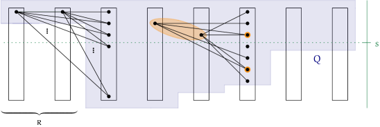
On the other blocks, where does not consist of a single vertex, we require that these blocks are large, of size at least . In addition we also require that all common neighborhoods are bounded on this large part. An illustration of a good rectangle can be found in Figure 3. The formal definition follows.
Definition 6.6 (Good rectangle).
Let be a -partite graph and let and . A rectangle is -good for if it satisfies the following properties.
-
1.
If , then ; otherwise .
-
2.
For all it holds that .
-
3.
For all of size at most and for all , has -bounded common neighborhoods from to .
On good rectangles the measure is tightly concentrated around the expected value. In Section 7 we prove the following concentration bound.
Lemma 6.7.
For constants and , for and satisfying and the following holds. If and is a -well-behaved graph, then any -good rectangle for with satisfies
In the remainder of this section we prove 6.3, assuming 6.7. As outlined in Section 3.4, we intend to decompose any rectangle into a small family of rectangles such that each rectangle in either contains few tuples, is a subrectangle of an edge axiom or is a good rectangle. The following lemma summarizes our claim.
Lemma 6.8.
Let be a -well-behaved graph, let , and for some large enough constant . Then any rectangle can be partitioned into a set of rectangles of size such that each satisfies that either
-
1.
is small: ,
-
2.
is a subrectangle of an edge axiom, or
-
3.
is -good for , where satisfies .
Before proving Lemma 6.8, let us first show how 6.3 follows. The idea of the proof is to apply Lemma 6.8 to a given rectangle to obtain a collection of rectangles. It holds that . By Lemma 3.5 there is a such that all small rectangles satisfy and similarly by 6.2 the same holds for that are a subrectangle of an edge axiom. Further, by our choice of parameters, the size of is small—we may think of it as . We can thus lower bound
| (6.20) |
6.7 states that the remaining good rectangles in the above sum have strictly positive value. Thus as claimed. In what follows we verify that this indeed holds for our choice of parameters.
Proof of 6.3.
Let be any rectangle. Our goal is to show that , for a sufficiently small constant . Let be as in the statement of the lemma and choose for sufficiently small constants and such that for it holds that . Let and . Note that for our choice of parameters it holds that , hence , and we may thus apply Lemma 6.8 with to the rectangle to obtain a family of size at most .
By 6.2, any subrectangle of an axiom has measure bounded by . Moreover, according to Lemma 3.5 each small rectangle has measure of magnitude at most
| (6.21) |
which is even smaller than the bound on axioms. Since , we conclude that the measure of all small rectangles and all subrectangles of axioms in add up, in magnitude, to at most , for a small enough constant .
Let us proceed to prove Lemma 6.8.
Proof of Lemma 6.8.
Let us describe a recursive decomposition procedure that can be applied to any rectangle .
If either is small, a subrectangle of an axiom or -good for some , then return . Otherwise decompose in the following recursive fashion.
-
1.
If there is a singleton such that , then we decompose into many rectangles as follows. Denote by the vertices in that are not a neighbor of and assume that they are in blocks . For we remove all tuples that contain the vertex : let so we can write
(6.22) Note that the rectangles partition . Add the to the partition as these are subrectangles of edge axioms and recursively decompose .
-
2.
If there is a block of size , then split into the rectangles
(6.23) and recursively decompose each of these rectangles.
-
3.
Let be the set of blocks of size greater than . Because is -well-behaved, by Item 2 of Definition 5.4, it holds that has -bounded error sets. In particular has an error set of size at most . Decompose into and as in Item 1. By definition the rectangle is -good and we may thus add it to the partition. Recursively decompose the rectangles .
This completes the description of the decomposition procedure. We need to argue that the decomposition created by above procedure is not too large, that is, of size . Let us start with a few observations.
Because is -well-behaved it holds that has -bounded common neighborhoods in every block (see Item 1 of Definition 5.4). Let be a rectangle with blocks of size and with the remaining vertices contained in the common neighborhood of these singletons. All such rectangles are small. Thus the decomposition procedure does not need to decompose such rectangles any further.
Whenever we decompose a rectangle in Items 2 and 3 all rectangles that we need to recursively decompose have one more singleton. Because we can stop decomposing after identifying singletons and in Items 2 and 3 we create at most many rectangles that require further decomposition we end up with at most many rectangles. We ignored the rectangles from Item 1 so far. But each rectangle that requires further decomposition from Items 2 and 3 results in at most another many rectangles from Item 1. Thus the size of the family of rectangles is bounded by . ∎
7 The Measure Is Concentrated on Good Rectangles
This section is devoted to proving 6.7 that states that the measure on good rectangles is very well concentrated. We restate it here for convenience.
See 6.7
Let us introduce some notation and state 6.7 once more in a more convenient form for what follows. Let be the star with center and leaves , that is, consists of the vertices and edges . For simplicity we denote by the star and for let .
Lemma 7.1.
For constants and , for and satisfying , the following holds. If and is a -well-behaved graph, then any -good rectangle for with satisfies
Proof of 6.7.
Recall that we defined our measure for a rectangle as
| (7.1) |
Hence Lemma 7.1 implies, for the appropriate parameters, that all -good rectangles for satisfy
Let us give some intuition for the statement of Lemma 7.1. Clearly, if , then we are showing that the measure of a rectangle is tightly concentrated around the expected value. Let us explain where the factor comes from.
Consider two blocks, say blocks and . For vertices and let us denote by the rectangle consisting of all tuples that contain as well as . According to 6.2, if there is no edge between and , then . Recall that the measure of the whole space is roughly —hence if there is an edge between vertices and as above, we expect that “compensates” for the value rectangles, that is, we expect that if the edge is present. More generally, for we expect to pick up a factor of for each edge that we condition on being present between a vertex in and another block in . Lemma 7.1 establishes that this is indeed how the measure behaves.
Let us consider an -good rectangle . For ease of exposition let us assume that , the other cases are analogous. In other words, we assume, for all , that it holds that , these vertices form a clique and all edges from the first vertices to any other vertex in are present.
Recall that is the family of graphs on labeled vertices with a vertex cover of size at most , and that denotes the set of graphs in the -boundary, as defined in Section 4. Finally, for two graphs and defined over the same vertex set we denote by the graph over containing all edges of that are not present in .
We prove Lemma 7.1 in three steps. First we split the sum of Fourier characters into two parts: the main sum and some boundary sums. In a second step we show that the boundary sums are negligible, i.e., that they add up to very little. In the final step we then show that the main sum is tightly concentrated around the expected value.
The following claim splits the sum of Fourier characters into the main sum and several boundary sums. We postpone the straightforward proof until after we prove Lemma 7.1.
Claim 7.2.
For as in Lemma 7.1 and any tuple it holds that
The sum with the factor in 7.2 is the so-called main sum. Intuitively most of the measure is in the main sum and it adds up to approximately times the size of , that is,
| (7.2) |
The latter sums in 7.2 with coefficients are the so-called boundary sums. All of these sums turn out to be tiny, that is, for and it holds that
| (7.3) |
Both of the bounds corresponding to (7.2) and (7.3), and stated formally below, are proven in Section 7.1. 7.2 together with these bounds will allow us to conclude that the measure is tightly concentrated around .
Let us first state the bound for the main sum. Intuitively we may think of the below lemma as a version of Lemma 6.4 that holds on a local part of the graph.
Lemma 7.3.
For as in Lemma 7.1 the following holds for and . If , then all -good rectangles satisfy
On the other hand, reminiscent of the edge axioms, we have that the boundary sums are quite small. Note that, in contrast to Lemma 6.5, the bound below depends on the size of the rectangle .
Lemma 7.4.
For as in Lemma 7.1 the following holds for any constant and , for and . Let , and . Then all -good rectangles satisfy that if , then
and, on the other hand, if , then the above sum is empty.
Assuming these statements the proof of Lemma 7.1 boils down to a sequence of syntactic manipulations.
Proof of Lemma 7.1.
We now proceed to prove 7.2.
Proof of 7.2.
Suppose and let us start by considering the edge . We first observe that for any such that , it holds that
| (7.8) |
by definition of a good rectangle as every tuple contains the edge . Let us write
| (7.9) |
Note that we can partition the set into two parts: the first part contains all the graphs in the boundary of , that is, graphs , and the second set contains all the remaining graphs. Note that graphs contained in the latter set satisfy that . Hence, for every , it holds that
| (7.10) | ||||
| (7.11) | ||||
If we continue to rewrite the first sum in the above fashion for edges we obtain
| (7.12) | ||||
By iteratively applying the above arguments to vertices we conclude that
| (7.13) | ||||
as claimed. ∎
7.1 Concentration of the Main Sum and Bounding the Boundary Sums
In this section we prove 7.3 and 7.4. We rely on the following lemma which guarantees bounded character sum on arbitrary good rectangles, regardless of size. This is in contrast to Item 4 of Definition 5.4 which only holds for small rectangles. The more general statement follows from the latter by splitting any large rectangle into many small rectangles while maintaining goodness so that Item 4 of Definition 5.4 holds for these small rectangles.
Lemma 7.5.
Let and be such that , and . If , is a -well-behaved graph and is a core graph, then all -good rectangles satisfy, for , that
We defer the proof of this lemma to Section 7.2. Before we proceed to prove 7.3 and 7.4 let us record two claims regarding vertex covers.
Claim 7.6.
Any minimum vertex cover of a graph contains all vertices of degree at least .
Proof.
Any vertex cover of that does not contain a vertex of degree at least must contain all neighbors of and hence is of size at least . ∎
Claim 7.7.
For and a graph on vertices it holds that if , then .
Proof.
If , then is the complete graph on vertices and the statement readily follows. Otherwise, as every vertex in has degree , it follows by 7.6 that the set is contained in any minimum vertex cover of . Since the vertices in have to cover the edges in , and since any vertex cover of is such that is a vertex cover of , we may conclude . ∎
Finally we also need to revisit our map as we need a good bound on the number of cores that the graphs containing are mapped to. Before stating the claim let us recall the construction of the map , as done in Section 4.2: given a graph with lexicographically first vertex cover we let be the lex first maximal set of vertices with a matching from to that covers all vertices in . Similarly we let be the lex first maximal set of vertices in with a matching from to covering all vertices in . Finally we define .
Lemma 7.8.
Let . If denotes the set of cores such that and , then it holds that
Proof.
We argue that we can encode elements of the set of cores by using few bits. Fix a core and let as in the construction of (see Section 4.2 and the discussion above). By definition we have that and .
According to 7.6 every vertex in is in any minimum vertex cover of and thus contained in ; the lex first one. Hence there are only vertices in to be specified. We spend bits to specify this set. Once we have specified this set we know that the lex smallest vertices outside are contained in by construction. With another bits we may thus encode the remaining vertices of . Similarly, for , we know that the lex smallest vertices outside are in . Hence bits suffice to specify .
At this point we know the relevant vertices of the core. It remains to encode the edges. Some edges are given: all edges from to the rest of the core are present. As such there are at most many edges left to be specified. The claim follows. ∎
With these claims at hand we are ready to prove 7.3 and 7.4. We start with 7.3 restated here for convenience.
See 7.3
Proof.
Let and observe that . Further using that for it holds that we may bound
| (7.14) | ||||
| (7.15) | ||||
| (7.16) |
where we appeal to 7.7 to obtain (7.15) and to the triangle inequality for (7.16). Since by Theorem 4.4 it holds that we may apply 7.5 with to the inner expressions to obtain the bound
| (7.17) |
Applying Lemma 7.8 along with the fact that allows us to conclude
| (7.18) | ||||
| (7.19) | ||||
| (7.20) |
where we used that , the bound and the fact that the final sum is a geometric series. This completes the proof of 7.3 modulo 7.5. ∎
In order to show that the magnitude of the boundary sums is small, we need to bound the number of core graphs that contain the edge set . The bound from Lemma 7.8 turns out to be insufficient as it is with respect to , that is, the vertex cover size outside the set ; as we can apply 7.5 with only, we get concentration with respect to the size of the vertex cover in the set . This is a problem as the vertex cover in the set may be considerably smaller than in the set . We overcome this difference in parameters by leveraging the difference in the exponential factors and as follows.
Claim 7.9.
Let , , , and . It holds that
Proof.
We first argue that the set over which we sum is not so large and then provide a lower bound on . These two bounds will together imply the claim.
Let . Given parameters and , we consider cores such that , , , and . We claim that there are at most
| (7.21) |
such core graphs. Indeed, it is enough to specify the vertices in a minimum vertex cover of , the other at most vertices in , and the edges between vertices in the identified minimum vertex cover of and .
In order to obtain a lower bound on , note that the edge set consists only of edges with exactly one endpoint in . Hence all edges that are in and that have both endpoints in are also in . These include edges between and . Note that all edges in have one endpoint in and thus
| (7.22) |
This implies that and therefore
| (7.23) |
This bound, however, is not good enough for us. We need to also count edges in that are adjacent to and that we have not considered yet. Note that these include all the edges in . Let be the neighbors of in the graph . In particular, we have that since . This implies that and therefore . Now note that it must be the case that is in every minimum vertex cover of ; otherwise we would have a minimum vertex cover of that either contains (and then would not be in the -boundary) or is not a vertex cover of the graph . This implies that . We may thus conclude that
| (7.24) |
Using the bounds in Equation 7.21 and Equation 7.24 we may write
| (7.25) | ||||
| (7.26) |
Since , we have that . Finally, we need to sum over all possible values of and . Since and , the statement follows. ∎
In the remainder of this section we prove that boundary sums are small. For convenience we restate the claim. See 7.4
Proof.
Let us first consider the case . For all such it holds that all graphs we sum over contain the edges . As vertex has degree at least and , according to 7.6, it holds that is contained in any minimum vertex cover of . This implies that there are no graphs satisfying that are also in the -boundary. Thus the considered sum is empty for .
We now assume . We can also assume as otherwise the edge is in any graph we consider and hence cannot be a boundary edge. Recall that , and let , and . Similar to the proof of 7.3, though this time we rely on Proposition 4.3, we may rewrite the boundary sum as
| (7.27) | ||||
| (7.28) |
We now focus on the inner two sums. Since we have that . By definition of a good rectangle, for all , the edges are present in thus . Let . Using that and we can derive that
| (7.29) | ||||
| (7.30) | ||||
| (7.31) | ||||
| (7.32) |
Appealing to the triangle inequality we may thus bound
| (7.33) | ||||
| (7.34) | ||||
Fix and let . Note that the characters we sum in Equation 7.34 solely depend on edges between blocks of size at least . We may thus apply 7.5 to the inner expressions and, using that and , we obtain
| (7.35) |
From Lemma 7.8 we know that there are at most many cores we sum over. The problem is that this bound does not depend on and hence applying Lemma 7.8 to Equation 7.34 does not readily result in the desired bound.
In order to bound the number of cores, we partition them according to the size of their minimum vertex cover. Note that by 7.6, if it must be the case by the definition of core graphs. Therefore, for such graphs , we have that , where the last equality follows from 7.7. Using that since , we can apply 7.9 to obtain that
| (7.36) | ||||
| (7.37) | ||||
| (7.38) |
where , we use that and, in order to apply 7.9, we use that . Note that, as , we have that . This allows us to bound .
Finally, because and the sum in (7.38) is a geometric series with common ratio and coefficient we may conclude that
| (7.39) |
as claimed. ∎
7.2 Bounds for All Good Rectangles
This section is devoted to the proof of 7.5. We rely on the following lemma.
Lemma 7.10.
Let be integers such that and let be a positive real number such that . Let be a set satisfying and be a family of subsets over of size , where each is of size at least . Then there is a partition of such that
-
1.
for all , and
-
2.
for each set and it holds that .
Proof.
We use the probabilistic method to show that a partition as claimed exists. Independently color each element in by a color in . Let denote color class .
Let us argue Item 1. By the multiplicative Chernoff bound we have that for a single , Item 1 holds except with probability . A union bound over the sets establishes that except with probability Item 1 holds.
To argue Item 2 we again appeal to the multiplicative Chernoff bound to see that for a fixed and the property holds except with probability . A union bound over the family and shows that Item 2 holds except with probability less than .
A final union bound shows the existence of a partition as claimed. ∎
As a corollary we can show that any good rectangle can be partitioned into many small good rectangles with only a slight loss in parameters.
Corollary 7.11.
Let and be such that , and , let and . If is a -good rectangle and , then there is a partition of into a set of at most rectangles such that each is -good and satisfies for all .
Proof.
This is a direct consequence of Lemma 7.10: fix such that . Apply Lemma 7.10 with , , , and being the common neighborhoods in of all tuples of size at most . Thus we get the bound and that every set in is of size at least . The bound on in the lemma statement has been chosen so that the conditions of Lemma 7.10 are satisfied.
Thus we obtain a partition of such that each set satisfies as required. Furthermore, each small tuple has a common neighborhood of size in the set . Here we used Item 3 of Definition 6.6 which states that has -bounded common neighborhoods into . Because the interval is contained in we have that each tuple has a -bounded common neighborhood in . Applying Lemma 7.10 iteratively in the above manner to each large block gives us the family in the statement. ∎
We are now ready to prove 7.5 restated here for convenience.
See 7.5
Proof.
We first apply Corollary 7.11 to an -good rectangle with to obtain a family of -good rectangles with the additional property that each block is bounded in size by . We can therefore write
| (7.40) | ||||
| (7.41) | ||||
| (7.42) |
where (7.41) follows directly from Item 4 of Definition 5.4 by noting that every is an -good rectangles such that for all , and that every -tuple has a unique -tuple extension in . ∎
8 Random Graphs Are Well-Behaved
In this section we prove that graphs sampled from are asymptotically almost surely -well-behaved. For convenience we recall the precise statement below.
See 5.5
Recall that Definition 5.4 consists of four properties: Item 1 states that the common neighborhood of small tuples behave as expected. When we focus our attention on a subgraph induced by a rectangle, we cannot expect that the common neighborhoods in this rectangle still behave as expected—we may for example have an isolated vertex in a rectangle. Item 2 of Definition 5.4 guarantees thus a slightly weaker property: it roughly states that every rectangle has only few small tuples whose common neighborhood is ill-behaved.
While the first two properties of Definition 5.4 are of combinatorial nature, the final two properties are more of analytical nature. Item 3 states that character sums over families are bounded for rectangles with large enough minimum block size. Once we consider smaller rectangles, things are not so well-behaved anymore. However, for certain rectangles, we can still guarantee a similar property: Item 4 of Definition 5.4 states that if the common neighborhoods of small tuples in a rectangle are well-behaved, then we can still guarantee that the mentioned character sums are bounded. In fact, this bound is in some sense tighter than the one in Item 3 as it actually depends on the size of the considered rectangle.
In Section 8.1 we start by proving that Items 1 and 2 of Definition 5.4 hold asymptotically almost surely. As previously mentioned, similar notions have been used in previous papers on the clique formula [BIS07, BGLR12, ABdR+21]. Our arguments towards Items 1 and 2 are heavily influenced by these papers, and some are essentially identical.
Once we established the combinatorial properties, in Section 8.2, we then prove the analytical Items 4 and 3 of Definition 5.4, modulo a probabilistic bound on the weighted sums of Fourier characters. Section 8.3 is dedicated to the proof of the probabilistic bound which, inspired by [AMP21], follows via an encoding argument applied to a high moment version of the Markov inequality.
8.1 Random Graphs Have Bounded Common Neighborhoods
In this section we prove that asymptotically almost surely satisfy Items 1 and 2 of Definition 5.4.
Lemma 8.1.
For any constant , any integer satisfying and the following holds for . Except with probability a graph has -bounded common neighborhoods in every block, for .
Proof.
Given a set of vertices , let be the indicator random variable of whether a vertex is in the common neighborhood of . Note that . Thus in expectation we have many common neighbors per block. Applying the multiplicative Chernoff bound we get that
| (8.1) |
Taking a union bound over all blocks and all sets of size less than or equal to we get
| (8.2) | ||||
| (8.3) |
which is exponentially small in . ∎
While all small sets have common neighborhoods of expected size in any block, this is not necessarily true for subsets of a block. For example, if consists of all non-neighbors of a vertex , then clearly does not have a neighborhood in of expected size. We can, nonetheless, show that for any large enough set there is a small set of vertices , which we refer to as the error set of , such that all small sets of vertices not intersection have a common neighborhoods in of expected size. The following lemma works out the precise dependency between the size of and the size of .
Lemma 8.2.
For all , , , and the following holds asymptotically almost surely for . For all , for all and for every subset of size , for , there is a set of size at most such that every tuple , , disjoint from and has a common neighborhood size in of expected size, that is, it holds that
Proof.
Given and , for some , we define a set such that for every tuple with and that is disjoint from and it holds that
| (8.4) |
Our goal is then to show that the probability of the event that there exists an , and a set of size at least such that is at most .
The set is constructed by including all tuples of that do not satisfy Equation 8.4. More formally, we first consider each possible tuple size and separately construct sets as follows. Let be an arbitrary but fixed maximal sequence of pairwise disjoint tuples, each of size , where each tuple either has too many or too few common neighbors in , that is, or for all . We define and .
Let . Note that if for all , then and
| (8.5) |
where we use that . We can therefore bound the probability that by bounding the probability that there exists an such that .
Fix an . The probability that a given tuple of of size has too many or too few common neighbors in can be bounded by the multiplicative Chernoff bound to obtain that
| (8.6) |
Note that the presence of edges between disjoint tuples and are independent events. Thus we can bound the probability that there there are at least many disjoint tuples that have too many or too few common neighbors in by
| (8.7) |
By taking a union bound over , and , and then for each and taking a union bound over , over the choices of of size , and over the choices for the tuples (of which there are at most ), we conclude that the probability that there exists an and a set of size at least such that is at most
| (8.8) | ||||
| (8.9) | ||||
| (8.10) |
as we wished to prove. ∎
Given a large rectangle we would like to argue that after removing the union of all error sets we are left with a rectangle in which all small tuples have common neighborhoods of expected size. To this end we rely on the following claim.
Claim 8.3.
Let and . Suppose we have a universe and a set satisfying . For any set satisfying it holds that
Proof.
Let us denote the size of by , the size of by and the size of by . It holds that
| (8.11) |
For the lower bound observe that it holds
| (8.12) |
where, for the final inequality, we used that . ∎
We are now ready to prove that, asymptotically almost surely, for , satisfies Item 2 of Definition 5.4 which states that for all , and , for a large enough constant , the graph has -bounded error sets, i.e., that for all rectangles satisfying or it holds that there exists a small set , , such that for all of size at most it holds that all tuples satisfy for all .
Corollary 8.4.
There exists a constant such that the following holds for all and integers satisfying and . A graph sampled from has asymptotically almost surely -bounded error sets for all and .
Proof.
Let and be such that if and otherwise. Our goal is to show that there exists a small set of vertices , , such that for all of size at most it holds that all tuples satisfy
for all .
Fix , and the parameters and . Note that by choosing it holds that . For each , let be the set, guaranteed to exist (asymptotically almost surely) by Lemma 8.2, of size at most such that for all of size at most it holds that all tuples satisfy
| (8.13) |
Note that to apply Lemma 8.2 we use the fact that for all , which follows since and .
Let . Since , we have that . Moreover, for all of size at most and all , it holds that all tuples satisfy
| (8.14) |
by 8.3 where we use the bound . Since and , the statement follows. ∎
8.2 Random Graphs Have Bounded Character Sums
In order to show that random graphs are asymptotically almost surely well-behaved, we rely on the following probabilistic bound on the weighted sums of Fourier characters, inspired by [AMP21].
Lemma 8.5.
Let be a non-empty graph over the vertex set with , and let be any matching in . Let be a rectangle such that for every edge it holds that . For any even , any and any function it holds that
where each edge in is sampled independently at random with probability .
It may be illustrative to consider the case when is a single edge, is the constant function, and . In this setting we obtain a bound on the absolute value of random variables taking values in uniformly at random. For some setting of parameters we essentially recover the Chernoff bound: we may, for example, set and to obtain the bound
| (8.15) |
which is essentially the bound that Chernoff guarantees.
The proof of 8.5 goes through a high moment version of the Markov inequality. After some standard manipulations of the resulting expressions we are left to bound the number of ways to map copies of the graph into such that every -tuple in is either mapped to at at least twice or not at all. We bound this quantity via an encoding argument.
The main idea of the encoding argument is to only consider the edges in the matching . Each such edge can be mapped in at least ways. As , we argue that it is beneficial to point to the other copy of that maps this edge to the same place. This drives the upper bound on the failure probability. The details of the argument are worked out in Section 8.3.
With this lemma in hand we are ready to prove the main result of this section.
Proof of 5.5.
Items 1 and 2 hold asymptotically almost surely by Lemma 8.1 and Corollary 8.4, respectively.
For Items 4 and 3 we will apply 8.5 to bound the probability that for a fixed core graph and rectangle that satisfy the conditions stated does not have bounded character sums over for . We will then apply a union bound over all such ’s and ’s.
We start by defining a function for every core , rectangle , graph and subset that maps tuples , for , to real numbers as
| (8.16) |
Observe that
| (8.17) | ||||
| (8.18) |
Note that only depends on , and , that is, it does not depend on the edges between vertices in . This will be crucial for our analysis as it implies that once we fix , , and we can determine whether is -bounded.
For a fixed , let be the event that is -bounded. By 8.5, we claim that for any if is -large, then for any it holds that
| (8.19) |
Indeed, this follows by rewriting the left hand-side according to Equation 8.17 to obtain
| (8.20) | ||||
and applying 8.5 for each fixed .
We are now ready to prove that asymptotically almost surely satisfies Items 4 and 3. Fix a core and a rectangle .
For Item 3 we may assume that is -large. Let and . By Item 1 has -bounded common neighborhoods in every block hence is -bounded for . Applying Equation 8.19 for this value of and for , and , we derive that the probability that does not have -bounded character sums over for is at most . We conclude Item 3 by taking a union bound over all cores of vertex cover at most , of which, according to Lemma 2.4, there are at most , and all rectangles, using the fact that and .
Item 4 follows by a similar argument. Further fix an integer , and a subset , let and . We assume is -small and -large. Note that if is such that for every , has -bounded common neighborhoods from to , then is -bounded for .
We can therefore apply Equation 8.19 with parameters , , , and , to obtain that the probability that does not have -bounded character sums over for is at most . Applying a union bound over all such that , all cores of vertex cover at most , all -small rectangles and all subsets we conclude that the probability that does not satisfy Item 4 is at most since, by Lemma 2.4, there are at most many core graphs, rectangles that are -small and only subsets . ∎
8.3 Probabilistic Bound on Sums of Fourier Characters
The rest of this section is dedicated to the proof of 8.5, restated here for convenience.
See 8.5
Proof.
In order to bound the probability we resort to a high moment version of the Markov inequality and conclude that
| (8.21) |
for even . For conciseness, let us write instead of and rewrite above expectation to obtain that
| (8.22) | ||||
| (8.23) | ||||
| (8.24) |
Observe that the magnitude of each expectation in Equation 8.22 is unless each edge appears at least twice in the product, in which case it is at most . Indeed, for it holds that
| (8.25) |
Therefore, given such that each edge appears at least twice, we have that
| (8.26) |
It remains to bound the number of tuples such that each edge appears at least twice. In more detail, we want to count the number of ordered sequences such that if is mapped to each tuple , then in the resulting multi-graph each edge appears at least twice.
To this end, let be the family of ordered sequences that give rise to such multi-graphs. In what follows we bound the cardinality of by an encoding argument: we encode each element of with few bits and thus establish that this set is small.
Let us fix one such sequence . Encoding each tuple separately is too costly. To minimize the bits needed we use the property that in the resulting multi-graph each edge is covered at least twice—in fact, we only use this property for edges in the matching. We encode the sequence as follows.
-
•
First, for each , we go through the edges of the th copy of in some fixed order. Suppose we consider an edge in the th copy of . If this edge has not been matched yet, then we write down an integer indicating that the tuples and map the vertices and to the same place. The edge of the th copy of is then said to be matched. Otherwise, if the edge of the th copy of has already been matched, then we continue with the next edge.
-
•
After completing above step we encode the tuples. We use the knowledge of the previous step: if we indicated that the th vertex of the tuples and are mapped to the same place, then we encode the target only once. More precisely, we encode the tuples as follows. Iterate over each and . If the th vertex of has already been mapped, then continue with the next vertex. Otherwise, we write down an integer indicating that the th vertex of is equal to . If the th vertex of has matched edges incident, then record the corresponding th vertices as mapped.
It should be evident that this procedure can be inverted, i.e., from the information written we can uniquely decode the sequence , provided we know the graph , the matching , the rectangle and the integer .
Let us tally the bits used in the above encoding. Suppose that in the first step we matched edges.
-
•
For each matched edge we wrote down bits for a total of bits, and
-
•
at most many bits in the second step: each matched edge reduces the total number of vertices to be mapped by (using that we only match edges in ). As for every edge it holds that , we see that the number of bits required in the second step of the encoding is reduced by each matched edge by at least bits.
Hence we need at most many bits to encode such a sequence of tuples. As we assumed that we conclude that
| (8.27) | ||||
| (8.28) |
Substituting this bound in Equation 8.21 results in the desired statement. ∎
9 Concluding Remarks
For we prove an essentially tight average-case coefficient size lower bound on Sherali-Adams refutations of the -clique formula for Erdős-Rényi random graphs with maximum clique of size . In fact, we obtain a lower bound on the sum of the magnitude of the coefficients appearing in a (general) Sherali-Adams refutation. The obvious problem left open is to prove an monomial size lower bound on Sherali-Adams refutations of the clique formula.
One possible avenue to prove such a monomial size lower bound is to argue that any Sherali-Adams proof of the clique formula can be converted into a proof of the same monomial size but with small coefficients. As shown in [GHJ+22] this is in general not possible and one would hence have to leverage the structure of the clique formula to argue that such a conversion exists. In fact, a slightly weaker statement would suffice: recall that our lower bound only counts the size of the coefficients of generalized monomials as well as of monomials multiplied by edge axioms. As such we would just need to be able to convert a general Sherali-Adams refutation into a refutation with low coefficients for such monomials.
In contrast to previous lower bounds for clique, our proof strategy is not purely combinatorial. It might be fruitful to obtain an explicit combinatorial description of —we believe this could potentially be used to prove average-case clique lower bounds for other proof systems, including resolution.
A strength of our lower bound approach is that it is quite oblivious to the encoding: one can introduce all possible extension variables depending on a single block and the lower bound argument still goes through. This is because the only property we require of a monomial is that the set of tuples whose associated assignment sets to non-zero is a rectangle. By extending in the natural manner to extension variables it is easy to see that is still a rectangle.
Our lower bound strategy seems to fail quite spectacularly once the edge probability is increased well beyond . More precisely, once , we fail to counter exponential in factors that arise from encoding the core graphs: as long as we can counter these with terms, where is the minimum block size of a good rectangle. As is clearly bounded by the block size , this approach fails once . We leave it as an open problem to extend our result to the dense setting.
We rely on rather unorthodox pseudorandomness properties of the underlying graph. It is natural to wonder whether these properties follow from a previously studied notion of pseudorandomness. Furthermore, it is wide open whether our lower bound can be made explicit. In particular, we have not investigated whether graphs that satisfy our pseudorandomness property can be constructed deterministically.
Another application of our pseudo-measure is in communication complexity. Suppose we consider the -player number-in-hand model, where player obtains a single node from block . The goal of the players is to find an edge missing in the induced subgraph by the tuple . Consider the leaves of such a communication protocol. Note that each leaf is associated with a subrectangle of an edge axiom. As the family of these associated rectangles partition the whole space, but , there must be at least leaves.
Finally, we have not investigated whether our technique can be used to obtain lower bounds for other proof systems. For example, is it possible that with similar ideas one could obtain tree-like cutting planes lower bounds with bounded coefficients? Possibly even with unbounded coefficients? The communication complexity view of the problem suggests that this may be a viable approach.
Acknowledgements
The authors are grateful to Albert Atserias, Per Austrin, Johan Håstad, Jakob Nordström, Pavel Pudlák, Dmitry Sokolov, Joseph Swernofsky, Neil Thapen and Marc Vinyals for helpful discussions and feedback. In particular we would like to thank Albert Atserias who observed that cores seem to be related to kernels.
We benefited from feedback of the participants of the Oberwolfach workshop 2413 “Proof Complexity and Beyond” and would like to thank the anonymous FOCS reviewers whose comments helped us improve the exposition in the paper considerably.
This work was supported by the Approximability and Proof Complexity project funded by the Knut and Alice Wallenberg Foundation. Part of this work was carried out while all authors were associated with KTH Royal Institute of Technology. Other parts were carried out while taking part in the semester program Lower Bounds in Computational Complexity in the fall of 2018 and the semster programs Meta-Complexity and Satisfiability: Extended Reunion in the spring of 2023 at the Simons Institute for the Theory of Computing at UC Berkeley.
Susanna F. de Rezende received funding from ELLIIT, from Knut and Alice Wallenberg grants KAW 2018.0371 and KAW 2021.0307, and from the Swedish Research Council grant 2021-05104. Aaron Potechin was supported by NSF grant CCF-2008920. Kilian Risse is supported by Swiss National Science Foundation project 200021-184656 “Randomness in Problem Instances and Randomized Algorithms”.
Appendix A Explicit Characterization of
Instead of implicitly describing as done in Section 4 we can describe this edge set explicitly as follows. Given a graph and a set of vertices , for every such that there is a matching from to that covers , we let be the set of vertices that could potentially be used to extend one of these matchings. More formally, is the set of vertices such that there is a matching from to that covers ; in this way, if any vertex is adjacent to , then there is a matching from to that covers . With this definition we can define formally as follows.
Definition A.1 ().
Let and let denote the objects from Algorithm 1 run on . For a set with a matching between and of size , we let be the set of vertices
and define
Lemma A.2.
For every it holds that if and only if for some .
Proof.
We first argue that given then for any it holds that . Let for some and denote by and the sets obtained by Algorithm 1 on . Note that has the same edges as on the vertices . Let us argue that a run of Algorithm 1 on results in the same sets , and .
-
1.
All edges in are incident to a vertex in and hence is a vertex cover of . Since is the lexicographically first minimum vertex cover of it must be the lexicographically first minimum vertex cover of .
-
2.
We now argue that the set is the lexicographically first maximal subset of with a matching in of size from to . To see this, let be the lexicographically first maximal set such that there is a matching in between and that covers , and suppose for the sake of contradiction that . This implies that either or is lexicographically smaller than . Let be the lexicographically first vertex in the symmetric difference of and . Note that it must be the case that (since either or is maximal and lexicographically smaller than ). Let be the vertex in that is matched to in . Note that cannot be in since the set would contradict the choice of . Moreover, it holds that hence is not in . But contradicts .
-
3.
Similarly, we argue that the set is the lexicographically first maximal subset disjoint of with a matching in of size from to . To see this, let be the lexicographically first maximal set such that there is a matching in between and that covers , and suppose for the sake of contradiction that . This implies that either or is lexicographically smaller than . Let be the lexicographically first vertex in the symmetric difference of and . Note that it must be the case that (since either or is maximal and lexicographically smaller than ). Let be the vertex in that is matched to in . Note that cannot be in since the set would contradict the choice of . Moreover, it holds that , hence is not in . But contradicts .
For the other direction, let and be the sets obtained by Algorithm 1 on , and let . Assume, for sake of contradiction, that contains an edge . We analyse four cases depending on where the endpoints of are located.
-
1.
If is not incident to a vertex in , then this contradicts the fact that is a vertex cover of .
-
2.
If both endpoints of are in then has different edges than on the vertices , contradicting that .
We are left to analyse the case when for some and . Note that since it must hold that or .
-
3.
If for some and (hence ), then there is a matching between and that covers . Since precedes lexicographically, this contradicts our choice of .
-
4.
If for some and (hence ), then there is a matching between and that covers . Since precedes lexicographically, this contradicts our choice of .
In each case, we obtained a contradiction and therefore we conclude that if then cannot contain an edge . This completes the proof of the lemma. ∎
References
- [ABdR+21] Albert Atserias, Ilario Bonacina, Susanna F. de Rezende, Massimo Lauria, Jakob Nordström, and Alexander A. Razborov. Clique is hard on average for regular resolution. J. ACM, 68(4):23:1–23:26, 2021.
- [AH19] Albert Atserias and Tuomas Hakoniemi. Size-Degree Trade-Offs for Sums-of-Squares and Positivstellensatz Proofs. In Amir Shpilka, editor, 34th Computational Complexity Conference (CCC 2019), volume 137 of Leibniz International Proceedings in Informatics (LIPIcs), pages 24:1–24:20, Dagstuhl, Germany, 2019. Schloss Dagstuhl–Leibniz-Zentrum fuer Informatik.
- [AMP21] Kwangjun Ahn, Dhruv Medarametla, and Aaron Potechin. Graph matrices: Norm bounds and applications, 2021.
- [BGLR12] Olaf Beyersdorff, Nicola Galesi, Massimo Lauria, and Alexander A. Razborov. Parameterized bounded-depth Frege is not optimal. ACM Transactions on Computation Theory, 4(3):7:1–7:16, September 2012. Preliminary version in ICALP ’11.
- [BHK+19] Boaz Barak, Samuel Hopkins, Jonathan Kelner, Pravesh K. Kothari, Ankur Moitra, and Aaron Potechin. A nearly tight sum-of-squares lower bound for the planted clique problem. SIAM Journal on Computing, 48(2):687–735, 2019.
- [BIS07] Paul Beame, Russell Impagliazzo, and Ashish Sabharwal. The resolution complexity of independent sets and vertex covers in random graphs. Comput. Complex., 16(3):245–297, 2007.
- [BT06] Andrej Bogdanov and Luca Trevisan. On worst-case to average-case reductions for NP problems. SIAM J. Comput., 36(4):1119–1159, 2006.
- [CHKX04] Jianer Chen, Xiuzhen Huang, Iyad A. Kanj, and Ge Xia. Linear FPT reductions and computational lower bounds. In Proceedings of the 36th Annual ACM Symposium on Theory of Computing (STOC ’04), pages 212–221, June 2004.
- [Coo71] Stephen A. Cook. The complexity of theorem-proving procedures. In Proceedings of the 3rd Annual ACM Symposium on Theory of Computing (STOC ’71), pages 151–158, May 1971.
- [DF95] Rodney Downey and Michael R. Fellows. Fixed-parameter tractability and completeness II: Completeness for W[1]. Theoretical Computer Science A, 141(1–2):109–131, April 1995.
- [DGGM20] Stefan S. Dantchev, Nicola Galesi, Abdul Ghani, and Barnaby Martin. Proof complexity and the binary encoding of combinatorial principles. CoRR, abs/2008.02138, 2020.
- [DM13] Stefan S. Dantchev and Barnaby Martin. Rank complexity gap for lovász-schrijver and sherali-adams proof systems. Comput. Complex., 22(1):191–213, 2013.
- [DRPR23] Susanna F. De Rezende, Aaron Potechin, and Kilian Risse. Clique is hard on average for unary sherali-adams. In 2023 IEEE 64th Annual Symposium on Foundations of Computer Science (FOCS), pages 12–25, 2023.
- [FHR+24] Yuval Filmus, Edward A. Hirsch, Artur Riazanov, Alexander Smal, and Marc Vinyals. Proving Unsatisfiability with Hitting Formulas. In Venkatesan Guruswami, editor, 15th Innovations in Theoretical Computer Science Conference (ITCS 2024), volume 287 of Leibniz International Proceedings in Informatics (LIPIcs), pages 48:1–48:20, Dagstuhl, Germany, 2024. Schloss Dagstuhl – Leibniz-Zentrum für Informatik.
- [FJK+18] Michael R. Fellows, Lars Jaffke, Aliz Izabella Király, Frances A. Rosamond, and Mathias Weller. What Is Known About Vertex Cover Kernelization?, pages 330–356. Springer International Publishing, Cham, 2018.
- [FMSV23] Yuval Filmus, Meena Mahajan, Gaurav Sood, and Marc Vinyals. MaxSAT resolution and subcube sums. ACM Transactions on Computational Logic, 24(1):1–27, January 2023.
- [GHJ+22] Mika Göös, Alexandros Hollender, Siddhartha Jain, Gilbert Maystre, William Pires, Robert Robere, and Ran Tao. Separations in proof complexity and TFNP. In 63rd IEEE Annual Symposium on Foundations of Computer Science, FOCS 2022, Denver, CO, USA, October 31 - November 3, 2022, pages 1150–1161. IEEE, 2022.
- [Hås99] Johan Håstad. Clique is hard to approximate within . Acta Mathematica, 182:105–142, 1999. Preliminary version in FOCS ’96.
- [HKT24] Pavel Hubáček, Erfan Khaniki, and Neil Thapen. TFNP Intersections Through the Lens of Feasible Disjunction. In Venkatesan Guruswami, editor, 15th Innovations in Theoretical Computer Science Conference (ITCS 2024), volume 287 of Leibniz International Proceedings in Informatics (LIPIcs), pages 63:1–63:24, Dagstuhl, Germany, 2024. Schloss Dagstuhl – Leibniz-Zentrum für Informatik.
- [Kar72] Richard M. Karp. Reducibility among combinatorial problems. In Complexity of Computer Computations, The IBM Research Symposia Series, pages 85–103. Springer, 1972.
- [Lau18] Massimo Lauria. Cliques enumeration and tree-like resolution proofs. Inf. Process. Lett., 135:62–67, 2018.
- [LPRT17] Massimo Lauria, Pavel Pudlák, Vojtěch Rödl, and Neil Thapen. The complexity of proving that a graph is Ramsey. Combinatorica, 37(2):253–268, April 2017. Preliminary version in ICALP ’13.
- [Mar08] Susan Margulies. Computer Algebra, Combinatorics, and Complexity: Hilbert’s Nullstellensatz and NP-complete Problems. PhD thesis, University of California, Davis, 2008.
- [MPW15] Raghu Meka, Aaron Potechin, and Avi Wigderson. Sum-of-squares lower bounds for planted clique. In Proceedings of the 47th Annual ACM Symposium on Theory of Computing (STOC ’15), pages 87–96, June 2015.
- [NP85] Jaroslav Nešetřil and Svatopluk Poljak. On the complexity of the subgraph problem. Commentationes Mathematicae Universitatis Carolinae, 026(2):415–419, 1985.
- [Pan21a] Shuo Pang. Large clique is hard on average for resolution. In Rahul Santhanam and Daniil Musatov, editors, Computer Science - Theory and Applications - 16th International Computer Science Symposium in Russia, CSR 2021, Sochi, Russia, June 28 - July 2, 2021, Proceedings, volume 12730 of Lecture Notes in Computer Science, pages 361–380. Springer, 2021.
- [Pan21b] Shuo Pang. SOS lower bound for exact planted clique. In Valentine Kabanets, editor, 36th Computational Complexity Conference, CCC 2021, July 20-23, 2021, Toronto, Ontario, Canada (Virtual Conference), volume 200 of LIPIcs, pages 26:1–26:63. Schloss Dagstuhl - Leibniz-Zentrum für Informatik, 2021.
- [PZ22] Aaron Potechin and Aaron Zhang. Bounds on the total coefficient size of nullstellensatz proofs of the pigeonhole principle and the ordering principle, 2022.
- [Ros08] Benjamin Rossman. On the constant-depth complexity of k-clique. In Cynthia Dwork, editor, Proceedings of the 40th Annual ACM Symposium on Theory of Computing, Victoria, British Columbia, Canada, May 17-20, 2008, pages 721–730. ACM, 2008.
- [Ros10] Benjamin Rossman. The monotone complexity of k-clique on random graphs. In 51th Annual IEEE Symposium on Foundations of Computer Science, FOCS 2010, October 23-26, 2010, Las Vegas, Nevada, USA, pages 193–201. IEEE Computer Society, 2010.
- [SA94] Hanif D. Sherali and Warren P. Adams. A hierarchy of relaxations and convex hull characterizations for mixed-integer zero—one programming problems. Discrete Applied Mathematics, 52(1):83–106, 1994.
- [Zuc07] David Zuckerman. Linear degree extractors and the inapproximability of max clique and chromatic number. Theory of Computing, 3(6):103–128, August 2007. Preliminary version in STOC ’06.