Invariant tensions from holography
 

Abstract

We revisit the problem of defining an invariant notion of tension in gravity. For spacetimes whose asymptotics are those of a Defect CFT we propose two independent definitions : Gravitational tension given by the one-point function of the dilatation current, and inertial tension, or stiffness, given by the norm of the displacement operator. We show that both reduce to the tension of the Nambu-Goto action in the limit of classical thin-brane probes. Subtle normalisations of the relevant Witten diagrams are fixed by the Weyl and diffeomorphism Ward identities of the boundary DCFT. The gravitational tension is not defined for domain walls, whereas stiffness is not defined for point particles. When they both exist these two tensions are in general different, but the examples of line and surface BPS defects in $d=4$ show that superconformal invariance can identify them.

Laboratoire de Physique de l’École Normale Supérieure,
CNRS, PSL Research University and Sorbonne Universités
24 rue Lhomond, 75005 Paris, France

1 Introduction

A key entry in the AdS/CFT dictionary [1, 2, 3] is the relation between the mass, $m_{0}$, of a point particle in the bulk and the scaling dimension, $\Delta$, of the dual CFT operator. For a free scalar particle in AdS_d+1

$$\Delta\,=\,{d\over 2}\,+\,\sqrt{(m_{0}{\ell})^{2}+{d^{2}\over 4}}\,=\,m_{0}{\ell}+{d\over 2}+{d^{2}\over 8m_{0}{\ell}}+\cdots\$$ (1.1)

where ${\ell}$ is the AdS radius which we set henceforth equal to one. In the world-line formalism one finds $\langle{\mathcal{O}}(x){\mathcal{O}}(y)\rangle\sim e^{-m_{0}\,{\mathfrak{D}}}$, where ${\mathcal{O}}$ is the dual CFT operator inserted at the points $x$ and $y$ on the Poincaré boundary, ${\mathfrak{D}}=2\log(|x-y|/\epsilon)$ is the geodesic distance between these points and $\epsilon$ is the boundary cutoff. This explains the leading term in the expansion (1.1). The next term comes from Gaussian quantum fluctuations, and subleading ones from the non-linearities of the point-particle action which are conveniently resummed by the Klein-Gordon equation.

Such corrections are negligible if the Compton wavelength of the particle is much smaller than the AdS radius,  $m_{0}^{-1}\ll 1$. In addition, for the point-particle description to stay valid the AdS radius must be much larger than the Schwarzschild radius, $r_{S}\sim G_{N}m_{0}\ll 1$. In the language of ref.[4] one may refer to the range $1\ll m_{0}\ll 1/G_{N}$ as that of heavy but not huge operators. The latter correspond to black-hole micro-states for which the world-line approximation breaks down and the geometry thickens, as illustrated below.

Figure 1: A ‘banana-shaped’ geometry (right) replaces the geodesic world-line (left)

  when $G_{n}m\gtrapprox 1$ . The AdS boundary is in grey. The broken line on the left is a virtual

  graviton that screens the bare mass parameter of the point-particle action.

Whether or not the dual ‘banana-shaped’ geometry is a smooth horizonless fuzzball [5], a bound state or a black hole, mass cannot be defined locally anymore. In the world-line formalism virtual gravitons screen the bare mass parameter $m_{0}$. But an invariant energy does exist in global AdS [6, 7], and it coincides (up to a Casimir subtraction) with the dilatation charge $\Delta$. The existence of this invariant charge makes it possible to count the microscopic bulk states in the dual CFT.

All this is well known. The question that we would like to address here is whether the holographic dictionary contains a similar entry for the tension of $p$-dimensional branes. A brane in AdS can be compact, in which case its only gravitational charge is energy, but it may also have infinite extent and intersect the boundary along a $p$-dimensional defect [8, 9, 10, 11]. It should in this case be possible to give an invariant definition of tension on the AdS boundary. When a dual Defect Conformal Field Theory (DCFT) exists, the definition should only depend on its data. As for point particles, it must also reduce to the bare Nambu-Goto tension, $T_{p}^{(0)}$, in the limit of a thin, heavy but not huge brane (i.e. when $1\ll T_{p}^{(0)}\ll G_{N}T_{p}^{(0)}$). We will argue that two natural candidates fit the bill:

(I) The integrated one-point function of the dilatation current,

$$\boxed{\,T_{p}^{\,(\footnotesize\rm I)}\,:=\,\bigl{(}{\,\scalebox{0.92}{$d-1$}\over\scalebox{0.92}{$d-p-1$}}\bigr{)}\,\oiint ds^{j}\,\langle\hskip-2.84526pt\langle{\mathcal{J}}_{j}\rangle\hskip-2.84526pt\rangle\ ;\,}$$ (1.2)

(II) The norm, $C_{D}$, of the displacement operator

$$\boxed{\,T_{p}^{\,(\footnotesize\rm II)}\,:=\,C_{D}\,{\pi^{p/2}\,\Gamma({p\over 2}\scalebox{0.95}{$+1$})\over(p+2)\,\Gamma(p+1)}\ .\,}$$ (1.3)

Here $\langle\hskip-2.84526pt\langle\cdots\rangle\hskip-2.84526pt\rangle$ denote DCFT correlation functions in $\mathbb{R}^{d}$, the defect spans a $\mathbb{R}^{p}$ subspace, and the integral is over the (hyper)sphere around the defect in the transverse $\mathbb{R}^{(d-p)}$. The dilatation current is ${\mathcal{J}}_{j}=x^{m}T_{mj}$, and the CFT stress tensor obeys the conservation equation

$$\partial_{m}T^{mj}=\delta^{(d-p)}(x)D^{j}$$ (1.4)

with $j$ labelling transverse directions. Eq.(1.4) fixes unambiguously the norm of the displacement operator $D^{j}$, which becomes a piece of DCFT data [12]. The two definitions are illustrated in figures 2 and 3.

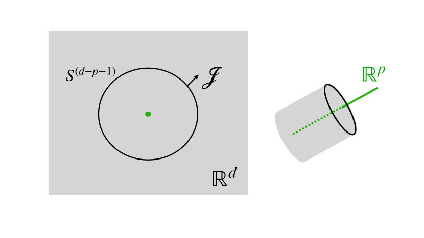
Figure 2: The gravitational tension is
the integral of the dilatation current $\mathcal{J}$
over a sphere around the defect.

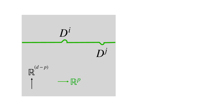
Figure 3: The inertial tension, or
‘stiffness’, is given by the 2-point
    function of the displacement.

Definition (I) is the natural extension of the dilatation charge $\Delta\simeq m_{0}$, to which it reduces for $p=0$. It is obtained from the graviton one-point function in AdS, so we refer to it as the gravitational tension. Note that in the case of domain walls both $\langle\hskip-2.84526pt\langle{\mathcal{J}}_{j}\rangle\hskip-2.84526pt\rangle$ and $d-p-1$ are zero, so the gravitational tension is not defined.

Definition (II), on the other hand, only makes sense for extended defects ($p>0$). It is a measure of stiffness, so we refer to it as inertial tension. For line defects ($p=1$) it is a multiple of the Bremsstrahlung function [13, 14, 15], and in the special case $d=2$, where a line defect is also an interface, it is proportional to the energy reflection coefficient [16]. Our interest in the definition of tension was spurred by holographic calculations in this latter context [17, 18, 19, 20], and part of our motivation for the present work was to generalise them to higher dimensions. We will not discuss boundaries in this work – viewed as limits of interfaces they have infinite tension [17].

We should note that definition (I) is reminiscent of earlier proposals for an invariant tension [21, 22, 23, 24, 25, 26] which also involve the asymptotic behaviour of the metric. These authors considered spacetimes whose asymptotics were ‘transverse flat’ or ‘planar empty AdS’, and they assumed the existence of an (exact or asymptotic) spacelike Killling isometry. Such an isometry is not required for our definitions. Although the AdS boundary in figures 2 and 3 is flat and the defect linear, all one really needs is that the radius of the sphere and the separation of the two displacement insertions be much smaller than all other DCFT scales.

Our main technical result will be to show, using Witten diagrams, that the right-hand sides of (1.2) and (1.3) reduce to the bare Nambu-Goto tension for classical probe branes. In this calculation normalisation factors matter and are subtle. We will fix them by verifying that the two-point function $\langle\hskip-2.84526pt\langle T^{mn}\,{\mathcal{D}}^{k}\rangle\hskip-2.84526pt\rangle$ obeys, in the above limit, the Weyl and diffeomorphism Ward identities [12] of the (putative) dual DCFT.

For defects of dimension $p=2$ or $4$ the displacement norm and one-point function of the stress tensor are related to Graham-Witten anomalies, see [27] for an updated summary. In the Nambu-Goto limit these can be obtained from the renormalised volume (alias ‘Willmore energy’) of minimal submanifolds [28, 29]. The use of Witten diagrams is a lowbrow method for computing such volumes for all $p$ and $d$.

The inertial and gravitational tensions are not, in general, equal beyond the thin-classical-probe limit. But for certain Wilson-line and surface defects in $d=4$ theories, superconformal Ward identities [30, 31] can be used to show that $T_{p}^{\footnotesize\rm(I)}=T_{p}^{\footnotesize\rm(II)}$ exactly. We conjecture that this should be true for large classes of superconformal defects. A similar conjecture was put forth in ref.[31] by extrapolating some known results to arbitrary $p$ and $d$. We will see that the two conjectures are actually identical.

The rest of the paper is organised as follows. In section 2 we show using Witten diagrams that (1.2) and (1.3) reduce to the Nambu-Goto tension for thin classical probes. We assume a natural but adhoc normalisation for the displacement source. In section 3 we calculate in the same limit the two-point function $\langle\hskip-2.84526pt\langle T^{mn}\,{\mathcal{D}}^{k}\rangle\hskip-2.84526pt\rangle$, and show that it obeys the DCFT Ward identities [12] which relate it to the displacement norm $C_{D}$ and to $\langle\hskip-2.84526pt\langle T^{mn}\rangle\hskip-2.84526pt\rangle$. This confirms the normalisations of the previous section. In section 4 we consider some specific defects, check that our calculations are consistent with results obtained by other methods, and comment on the quantum and gravitational corrections. Section 5 explains how supersymmetry can protect the relation $T_{p}^{\footnotesize\rm(I)}=T_{p}^{\footnotesize\rm(II)}$ from such corrections  and compares our conjecture to that of ref.[31]. This part deserves further study. The constraints on DCFT correlation functions are reviewed, for the reader’s convenience, in appendix A.

2 Nambu-Goto probes

To show that the right-hand sides of (1.2) and (1.3) reduce to the Nambu-Goto tension for thin classical probes we will use Witten diagrams [3, 32]. These have been applied to DCFT [33, 34, 35, 36, 37, 38, 39, 40] mostly in order to compare to exact results (from localisation and integrability) for superconformal Wilson lines. Our calculations are simpler but the focus is different. We are mainly concerned with the normalisation of bulk and defect sources.

2.1 Inertial tension

We begin with the definition (1.3). The norm of the displacement operator is read from the two-point function

$$\langle\hskip-2.84526pt\langle D^{i}(\vec{\tau})D^{j}(\vec{\tau}^{\,\prime})\rangle\hskip-2.84526pt\rangle\ =\ {C_{D}\,\delta^{ij}\over|\vec{\tau}-\vec{\tau}^{\,\prime}|^{\,2p+2}}\ ,$$ (2.1)

where $\vec{\tau}$ and $\vec{\tau}^{\,\prime}$ are points on the defect. Both the norm of $D^{j}$ and its scaling dimension, $\Delta=p+1$, are part of the DCFT data. The first task is to compute them on the gravity side.

The metric of Euclidean AdS_d+1 in Poincaré coordinates is

$$ds^{2}={\delta_{\mu\nu}\,dy^{\mu}dy^{\nu}\over(y^{0})^{2}}\qquad{\rm with}\quad\mu,\nu=0,1,\cdots,d\ \ .$$ (2.2)

The static brane sits at $y^{j}=0$ for $j=p+1,\cdots,d$ . It breaks the AdS_d+1 isometries to SO $(1,p+1)\times$ SO $(d-p)$ , but this residual symmetry does not act simply on the coordinates $y^{\mu}$. As realized in [33], the system of coordinates in which the residual isometries are manifest is 

$$y^{0}\,=\,x^{0}\,\Bigl{(}{1-{1\over 4}|x_{\perp}|^{2}\over 1+{1\over 4}|x_{\perp}|^{2}}\Bigr{)}\ ,\quad y^{a}=x^{a}\quad{\rm for}\quad a=1,\cdots,p$$

$$\quad\hskip-8.53581pt\quad{\rm and}\quad y^{j}\,=\,x^{0}\,\Bigl{(}{x^{j}\over 1+{1\over 4}|x_{\perp}|^{2}}\Bigr{)}\quad{\rm for}\quad j=p+1,\cdots,d\$$ (2.3)

with $|x_{\perp}|^{2}=\sum_{j}x^{j}x^{j}$. The metric in these coordinates reads

$$ds^{2}\,=\,{\delta_{\alpha\beta}\,dx^{\alpha}dx^{\beta}\over(x^{0})^{2}}\Bigl{(}{1-{1\over 4}|x_{\perp}|^{2}\over 1+{1\over 4}|x_{\perp}|^{2}}\Bigr{)}^{2}\,+\,{\delta_{ij}\,dx^{i}dx^{j}\over(1+{1\over 4}|x_{\perp}|^{2})^{2}}\ .$$ (2.4)

The unbroken SO $(1,p+1)$ acts now only on the $x^{\alpha}$, not the $x^{j}$.

Let $X^{\mu}(\tau)$ be the embedding of the $p$-brane in AdS_d+1. The Nambu-Goto action is proportional to the bare tension $T_{p}^{(0)}$,

$$I_{\rm NG}\,=\,T_{p}^{(0)}\hskip-1.42262pt\int d^{\,p+1}\tau\,\sqrt{{\rm det}(\hat{g}_{\alpha\beta})}\ \quad{\rm where}\quad\hat{g}_{\alpha\beta}=g_{\mu\nu}(X){\partial X^{\mu}\over\partial\tau^{\alpha}}{\partial X^{\nu}\over\partial\tau^{\beta}}$$ (2.5)

is the induced world-volume metric. Working in the static gauge, $X^{\alpha}=\tau^{\alpha}$, and expanding in small transverse fluctuations gives

$$I_{\rm NG}=T_{p}^{(0)}\hskip-2.56073pt\int\hskip-1.70717ptd^{\,p+1}\tau\,\sqrt{\bar{g}}\,\Bigl{[}1+\scalebox{0.95}{${1\over 2}$}\sum_{j}(\bar{g}^{\alpha\beta}\partial_{\alpha}X^{j}\partial_{\beta}X^{j}+\scalebox{0.9}{$(p+1)$}X^{j}X^{j})+\cdots\Bigr{]}\,.$$ (2.6)

Here $\bar{g}_{\alpha\beta}=\delta_{\alpha\beta}/(\tau^{0})^{2}$ is the metric of AdS_p+1 and the dots are terms quartic or higher in $X^{j}$. These contribute quantum corrections to the invariant tension that are suppressed by inverse powers of $T_{p}^{(0)}$. The action (2.6) describes $(d-p)$ scalar fields with mass $m^{2}=p+1$ living in AdS_p+1. From the relation $m^{2}=\Delta(\Delta-p)$ one sees that the dual operators have $\Delta=p+1$ , which is the expected dimension of $D^{j}$ [33].

We extract $C_{D}$ following the standard AdS/CFT recipy [32]. The on-shell $p$-brane coordinates are given at leading order by

$$X^{j}(\tau^{0},\vec{\tau})=\int d^{p}\tau^{\prime}\,K_{\Delta}(\tau^{0},\vec{\tau}\,;\,{\vec{\tau}^{\,\prime}})\,X^{j}(0,\vec{\tau}^{\,\prime})\ ,$$ (2.7)

where $\vec{\tau},\vec{\tau}^{\,\prime}$ are $p$-component vectors and

$$K_{\Delta}(\tau^{0},\vec{\tau}\,;\,{\vec{\tau}^{\,\prime}})\,=\,{\Gamma(\Delta)\over\pi^{p\over 2}\Gamma(\Delta-{1\over 2}p)}\,\biggl{[}{\tau^{0}\over(\tau^{0})^{2}+|\vec{\tau}-\vec{\tau}^{\,\prime}|^{2}}\biggr{]}^{\Delta}\$$ (2.8)

is the usual bulk-to-boundary propagator normalised in order to approach $\epsilon^{p-\Delta}\,\delta^{(p)}({\vec{\tau}-\vec{\tau}^{\,\prime}})$ in the limit $\tau^{0}=\epsilon\to 0$ . The generating functional of the DCFT is found by inserting (2.7) in the Nambu-Goto action,

$${\mathcal{Z}}={1\over 2}T_{p}^{(0)}{\scalebox{0.9}{$(2\Delta-p)$}\Gamma(\Delta)\over\pi^{p/2}\Gamma(\Delta-{1\over 2}p)}\int\hskip-1.70717ptd^{p}\tau\hskip-1.70717pt\int\hskip-1.70717ptd^{p}\tau^{\,\prime}\,X^{i}\scalebox{0.9}{$(0,\vec{\tau})$}\,X^{j}\scalebox{0.9}{$(0,\vec{\tau}^{\,\prime})$}\,{\delta^{ij}\over|\vec{\tau}-\vec{\tau}^{\,\prime}|^{\,2p+2}}\,,$$ (2.9)

with $X^{j}\scalebox{0.9}{$(0,\vec{\tau})$}$ the renormalised sources for the dual operators which we take to be the $D^{j}$. Eq.(2.9) differs from the naive on-shell action by an extra factor $(2\Delta-p)/\Delta$ which will be important for us here. It was first noticed in homogeneous CFTs by insisting that the regulated action be consistent with conformal Ward identities [32], and it was later shown to arise from the boundary limit of the bulk-to-bulk propagator [41, 42].

Setting $\Delta=p+1$ in (2.9) leads to the following relation between $C_{D}$ and the Nambu-Goto tension

$$\boxed{C_{D}=T_{p}^{(0)}\,{(p+2)\Gamma(p+1)\over\pi^{p/2}\Gamma({p\over 2}+1)}\,+\cdots\ }$$ (2.10)

with dots standing for the quantum and gravitational corrections that we neglected. Comparing eq.(2.10) to eq.(1.3) we see that $T_{p}^{\,(\footnotesize\rm II)}=T_{p}^{(0)}+\cdots$, as announced in the introduction.

But there are reasons to feel uneasy about this calculation. How do we actually know that $X^{j}(0,\vec{\tau})$ is the properly-normalised source of the displacement operator ? This should be fixed by the conservation eq. (1.4) which relates $D^{j}$ to $T^{mn}$, and hence the brane coordinates to the graviton. The relative normalisation of these latter is fixed by their transformation under diffeomorphisms, $\delta g_{\mu\nu}=\nabla_{\mu}\xi_{\nu}+\nabla_{\nu}\xi_{\mu}$ and $\delta X^{\mu}=\xi^{\mu}(X)$. But the Fefferman-Graham expansion of the metric is singular in the coordinates $x^{\mu}$, and the existence of an invariant regulator is not clear. Alternatively, one may argue following ref.[32], that the normalisation of the sources in (2.9) is determined by conformal Ward identities in AdS_p+1. But contrary to the homogeneous CFTs considered in this reference, the defect does not have its proper stress-energy tensor.

Despite these doubts eq.(2.10) turns out to be correct. We will show this using the DCFT Ward identities in section 3.

2.2 Gravitational tension

First we turn to the calculation of the gravitational tension. This depends on the one-point function of the bulk stress tensor which is fixed, up to an undetermined parameter $a_{\rm T}$, by the unbroken conformal symmetry. The result [12] (see also appendix A) reads

$$\langle\hskip-2.84526pt\langle T^{\,ab}\rangle\hskip-2.84526pt\rangle\,=\,a_{\rm T}\,\bigl{(}{\scalebox{0.95}{$d-p-1$}\over d}\bigr{)}\,{\delta^{ab}\over|x_{\perp}|^{d}}\ ,\qquad\langle\hskip-2.84526pt\langle T^{\,aj}\rangle\hskip-2.84526pt\rangle\,=\,0\ ,$$ (2.11a)

$$\ \quad\langle\hskip-2.84526pt\langle T^{\,ij}\rangle\hskip-2.84526pt\rangle\,=\,a_{\rm T}\,\Biggl{[}\,{x^{i}x^{j}\over|x_{\perp}|^{d+2}}\,-\,\bigl{(}{\scalebox{0.95}{$p+1$}\over d}\bigr{)}{\delta^{\,ij}\over|x_{\perp}|^{d}}\,\Biggr{]}\ \ .$$ (2.11b)

One can verify that $\langle\hskip-2.84526pt\langle T^{\,mn}\rangle\hskip-2.84526pt\rangle$ is traceless and conserved. Positivity of the energy density in the Lorentzian theory requires $a_{\rm T}$ to be negative. From eq.(2.11b) we find the radial component of the dilatation current in the transverse space

$${x^{m}x^{j}\over|x_{\perp}|}\,\langle\hskip-2.84526pt\langle T_{\,mj}\rangle\hskip-2.84526pt\rangle\,=\,{a_{\rm T}\over|x_{\perp}|^{d-1}}\,\bigl{(}{\scalebox{0.91}{$d-p-1$}\over d}\bigr{)}\ .$$ (2.12)

Integrating over the sphere in the definition (1.2) gives

$$\boxed{T_{p}^{\,(\footnotesize\rm I)}\,=\,-a_{\rm T}\,\,{2\,\pi^{(d-p)/2}\scalebox{0.92}{$(d-1)$}\over\Gamma(\scalebox{0.92}{${1\over 2}(d-p)$})\,d}\ .}$$ (2.13)

This expresses $T_{p}^{\,(\footnotesize\rm I)}$ in terms of the DCFT parameter $a_{\rm T}$. As already noted in the introduction, $a_{\rm T}=0$  for defects of codimension-one for which the above definition of tension fails.

We want now to calculate $a_{\rm T}$ in the thin-brane limit. To this end let $g_{\mu\nu}=\bar{g}_{\mu\nu}+h_{\mu\nu}$ with $\bar{g}_{\mu\nu}$ the metric of the bulk AdS. To ensure a smooth Fefferman-Graham expansion we must use the Poincaré coordinates $y^{\mu}$ for the graviton. The Fefferman-Graham expansion of defect fields, on the other hand, is regular in the coordinates $x^{\mu}$, whence the difficulties of regularisation mentioned in the previous subsection. Fortunately at the order at which we will work the change of coordinates (2.3) is simple,

$$y^{\alpha}=x^{\alpha}\,(1+O(x_{\perp}^{2}))\,\quad{\rm and}\quad y^{j}=x^{0}x^{j}\,(1+O(x_{\perp}^{2}))\ .$$ (2.14)

Thus, up to corrections of order $O(x_{\perp}^{2})$, the static-gauge parametrisation is unchanged and we only need to rescale the transverse brane coordinates, $Y^{j}=\tau^{0}\,X^{j}$. Furthermore, the usual ultraviolet cutoffs of AdS_d+1 and AdS_p+1 are the same at this leading order, $x^{0}=y^{0}=\epsilon$. Expanding the Nambu-Goto action (2.5) in powers of $h_{\mu\nu}$ and $Y^{j}$, and keeping only the terms of order $O(h)$ and $O(hY^{j})$, we find

$$I_{\rm NG}\ =\ \scalebox{0.95}{${1\over 2}$}\,T_{p}^{(0)}\int d^{\,p+1}\tau\,\sqrt{\bar{g}}\,\bar{g}^{\alpha\beta}\,\delta\hat{g}_{\alpha\beta}$$

$${\rm with}\quad\ \ \delta\hat{g}_{\alpha\beta}=(1+Y^{j}\partial_{j})h_{\alpha\beta}+h_{\alpha j}\partial_{\beta}Y^{j}+h_{\beta j}\partial_{\alpha}Y^{j}+\cdots\ .$$ (2.15)

Note that after replacing $Y^{j}$ by $\tau^{0}X^{j}$ manifest covariance is lost. This is because the metric perturbation transforms non-covariantly under the isometries of AdS_p+1.

The leading contribution to $\langle\hskip-2.84526pt\langle T^{\,mn}\rangle\hskip-2.84526pt\rangle\,$ comes from the graviton tadpole in (2.15). This simplest Witten diagram is shown in figure 4. It has a bulk-to-boundary graviton propagator integrated over the world-volume of the static $p$-brane. The graviton propagator reads [3, 32, 43]

$$K_{\,\mu\nu}^{\,mn}(x,y)\,=\,{C^{[2]}_{\Delta}\over(y_{0})^{\,2}}\,\bigl{(}{y^{0}\over|x-y|^{2}}\bigr{)}^{\Delta}\,J_{\mu r}(x-y)J_{\nu s}(x-y)P^{\,rs;\,mn}\$$ (2.16)

where $x=(0,\vec{x})$ is the point on the boundary,

$$C^{[2]}_{\Delta}={2\scalebox{0.95}{$(\Delta+1)$}\Gamma\scalebox{0.95}{$(\Delta-1)$}\over\pi^{d/2}\Gamma\scalebox{0.95}{$(\Delta-d/2)$}}\ ,\quad J_{\mu\nu}(z)=\delta_{\mu\nu}-{2z_{\mu}z_{\nu}\over z^{2}}\$$ (2.17)

$$\ \ \ {\rm and}\quad P^{\,rs;\,mn}\,=\,{1\over 2}(\delta^{rm}\delta^{sn}+\delta^{rn}\delta^{sm})-{1\over d}\,\delta^{rs}\delta^{mn}\ .$$ (2.18)

Recall that in our conventions $\mu,\nu\in[0,d]$ are bulk indices whereas $m,n,r,s\in[1,d]$ are boundary ones. The above propagator is valid for a spin-2 field of any mass, the massless graviton has $\Delta=d$. 

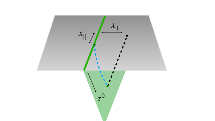
Figure 4: The Witten diagrams calculated in this and the following section. The graviton propagator (broken black line) and the displacement-field propagator (broken blue line) stretch from the thin brane in the AdS interior to a boundary point in the bulk, respectively on the defect. When the only external leg is the graviton, $x_{\parallel}$ can be set to zero.

The tadpole in (2.15), with the AdS_p+1 metric $\bar{g}_{\alpha\beta}=(\tau_{0})^{-2}\,\delta_{\alpha\beta}$, gives

$$\langle\hskip-2.84526pt\langle T^{\,mn}(x)\rangle\hskip-2.84526pt\rangle\,=\,-{T_{p}^{(0)}\over 2}\int{d^{p+1}\tau\over(\tau_{0})^{p-1}}\,\delta^{\alpha\beta}K_{\,\alpha\beta}^{\,mn}(x,\tau)\,.$$ (2.19)

Without loss of generality we take the boundary point to be at $x^{a}=0$. The point in the interior lies on the brane at $y^{\mu}=(\tau^{\alpha},0)$. We perform the index contractions in two steps. Frst

$$\delta^{\alpha\beta}J_{\alpha r}(x-y)J_{\beta s}(x-y)\,=\,\delta_{rs}^{\,\parallel}+{4z_{r}z_{s}\,|\tau|^{2}\over|z|^{4}}+{2(\tau_{r}z_{s}+z_{r}\tau_{s})\over|z|^{2}}\ ,$$ (2.20)

where $\delta_{rs}^{\,\parallel}$ is the Knonecker symbol in the subspace spanned by the defect, $z^{\mu}=x^{\mu}-y^{\mu}=(-\tau^{\alpha},x^{j})$ and $|z|^{2}=|\tau|^{2}+|x_{\perp}|^{2}$. Contracting next with the tensor $P^{\,rs;\,mn}$ and noting that $\delta^{rs}z_{r}z_{s}=|z|^{2}-(z_{0})^{2}$ gives

$$\delta^{\alpha\beta}J_{\alpha r}J_{\beta s}\,P^{\,rs;\,mn}\,=\,\delta^{\,mn}_{\,\parallel}+{4z^{m}z^{n}\,|\tau|^{2}\over|z|^{4}}+{2(\tau^{m}z^{n}+z^{m}\tau^{n})\over|z|^{2}}$$

$$\quad\quad\quad-{1\over d}\,\delta^{mn}\Bigl{[}\,p+{8|\tau|^{2}\over|z|^{2}}-{4(\tau_{0})^{2}|\tau|^{2}\over|z|^{4}}-{4(\tau_{0})^{2}\over|z|^{2}}\Bigr{]}\ .$$ (2.21)

For the transverse components $\langle\hskip-2.84526pt\langle T^{\,ij}\rangle\hskip-2.84526pt\rangle$ the above tensor structure reads

$${4x^{i}x^{j}\,|\tau|^{2}\over|z|^{4}}-{1\over d}\,\delta^{ij}\Bigl{[}\,p+{8|\tau|^{2}\over|z|^{2}}-{4(\tau_{0})^{2}|\tau|^{2}\over|z|^{4}}-{4(\tau_{0})^{2}\over|z|^{2}}\Bigr{]}\ .$$ (2.22)

The mixed components $\langle\hskip-2.84526pt\langle T^{\,aj}\rangle\hskip-2.84526pt\rangle$ vanish by $SO(p)$ symmetry, and in computing $\langle\hskip-2.84526pt\langle T^{\,ab}\rangle\hskip-2.84526pt\rangle$ one can replace for the same reason

$$\tau^{a}\tau^{b}\ \to\ {\delta^{ab}\over p}\,|\vec{\tau}|^{2}\ .$$

The integrand in eq.(2.19) thus only depends on $|\vec{\tau}|^{2}$ and $\tau_{0}$.

It is simplest to extract the DCFT parameter $a_{\rm T}$ by looking at the term proportional to $x^{i}x^{j}$. Inserting (2.22) in (2.19) and comparing with the one-point function (2.11b) gives

$$-{a_{\rm T}\over|x_{\perp}|^{d+2}}\,=\,{2\,T_{p}^{(0)}}\,C^{[2]}_{d}\int{d^{p+1}\tau\over(\tau_{0})^{p-d+1}}\,{|\tau|^{2}\over(|\tau|^{2}+|x_{\perp}|^{2})^{d+2}}\ .$$ (2.23)

The integral is computed using Schwinger’s trick as follows:

$$-{a_{\rm T}\over|x_{\perp}|^{d+2}}\,=\,{2\,T_{p}^{(0)}}\,C^{[2]}_{d}\int{d\tau_{0}\,d^{\,p}\tau\over(\tau_{0})^{p-d+1}}\,{(\tau_{0})^{2}+|\vec{\tau}|^{2}\over\bigl{(}(\tau_{0})^{2}+|\vec{\tau}|^{2}+|x_{\perp}|^{2}\bigr{)}^{d+2}}$$

$$=\,{2\,T_{p}^{(0)}\,C^{[2]}_{d}\over\Gamma(\scalebox{0.93}{$d+1$})}\int ds\,s^{d}\bigl{(}1-{|x_{\perp}|^{2}\,s\over d+1}\,\bigr{)}\,e^{-s|x_{\perp}|^{2}}\hskip-3.69885pt\int{d\tau_{0}\,d^{p}\tau\over(\tau_{0})^{p-d+1}}\,e^{-s(\tau_{0})^{2}-s|\vec{\tau}|^{2}}$$

$$=\,{T_{p}^{(0)}\,C^{[2]}_{d}\over\Gamma(\scalebox{0.93}{$d+1$})}\,\Gamma\scalebox{1.16}{$({d-p\over 2})$}\pi^{p/2}\int ds\,s^{d/2}\bigl{(}1-{|x_{\perp}|^{2}\,s\over d+1}\bigr{)}\,\,e^{-s|x_{\perp}|^{2}}$$

$$=\,{1\over|x_{\perp}|^{d+2}}{T_{p}^{(0)}\,C^{[2]}_{d}\over\Gamma(\scalebox{0.93}{$d+1$})}\,\Gamma\scalebox{1.06}{$({d-p\over 2})$}\pi^{p/2}\,{\Gamma\scalebox{1.16}{$({d\over 2}+1)$}\,d\over 2(d+1)}\ .$$

Inserting the expression for $C^{[2]}_{d}$ from (2.17) leads after a little algebra to

$$\boxed{-a_{\rm T}\,=\,{T_{p}^{(0)}\,\Gamma(\scalebox{1.1}{${d-p\over 2}$})\,d\over 2\,\scalebox{0.92}{$(d-1)$}\,\pi^{(d-p)/2}}+\cdots\ }$$ (2.24)

This expresses the DCFT parameter $a_{\rm T}$ in terms of the Nambu-Goto tension in the classical thin-brane probe limit. Comparing to eq.(2.13) we see that $T_{p}^{\,(\footnotesize\rm I)}=T_{p}^{(0)}+\cdots$ as announced.

The terms in $\langle\hskip-2.84526pt\langle T^{\,mn}\rangle\hskip-2.84526pt\rangle$ proportional to $\delta^{ab}$ and $\delta^{ij}$ can be computed similarly and have the general form (2.11a, 2.11b) dictated by conformal symmetry. We leave this as an exercise for the reader, and move on to the more involved calculation of the two-point function $\langle\hskip-2.84526pt\langle T^{\,mn}\,D^{j}\rangle\hskip-2.84526pt\rangle$.

3 Ward identities

We have explained in section 2.1 why normalising the displacement operator in Witten diagrams is tricky. We will now settle the issue by checking the DCFT Ward identities that have been derived in ref.[12]. They are of the form $\langle\hskip-2.84526pt\langle TD\rangle\hskip-2.84526pt\rangle\,\sim\,\langle\hskip-2.84526pt\langle T\rangle\hskip-2.84526pt\rangle\,+\langle\hskip-2.84526pt\langle DD\rangle\hskip-2.84526pt\rangle\,$  and fix therefore unambiguously the normalisations of both $D^{j}$ and $T^{mn}$ .

3.1 The DCFT identities

The two-point function $\langle\hskip-2.84526pt\langle T^{\,mn}\,D^{j}\rangle\hskip-2.84526pt\rangle$ is determined by the unbroken conformal and rotation symmetry modulo three unknown parameters $\mathfrak{b}_{1,2,3}$ (which are called $b_{\rm TD}^{1,2,3}$ in ref.[12]). This is most easily derived in the lightcone formalism as reviewed in appendix A. The result is

$$\langle\hskip-2.84526pt\langle T^{mn}(x)D^{j}(0)\rangle\hskip-2.84526pt\rangle\,=\,{|x_{\perp}|^{p-d}\over|x|^{2p+2}}\,F^{mn;\,j}(x)\qquad{\rm with}$$ (3.1)

$$F^{ab;\,j}(x)=\,{1\over d}[\scalebox{0.92}{$(d-p-1)\mathfrak{b}_{2}-\mathfrak{b}_{1}$}]\,{\delta^{ab}x^{j}}+\,\scalebox{0.92}{$4\mathfrak{b}_{1}$}\,{x^{a}x^{b}x^{j}|x_{\perp}|^{2}\over|x|^{4}}\,\,\,,$$ (3.2a)

$$F^{bi;\,j}(x)={\,}-\mathfrak{b}_{3}\,{\delta^{ij}x^{b}{|x_{\perp}|^{2}\over|x|^{2}}}+[\scalebox{0.92}{$4\mathfrak{b}_{3}-2\mathfrak{b}_{1}$}]\,{x^{i}x^{j}x^{b}\over|x|^{2}}+\scalebox{0.92}{$4\mathfrak{b}_{1}$}\,{x^{i}x^{j}x^{b}|x_{\perp}|^{2}\over|x|^{4}}\,\,\,,$$ (3.2b)

$$F^{ik;\,j}(x)=\,-{1\over d}[\scalebox{0.92}{$(p+1)\mathfrak{b}_{2}+\mathfrak{b}_{1}$}]\,\delta^{ik}{x^{j}}+{\mathfrak{b}_{3}\over 2}\,\delta^{j(i}x^{k)}\bigl{(}{\scalebox{0.99}{$1$}}-{\scalebox{0.87}{$2$}|x_{\perp}|^{2}\over|x|^{2}}\bigr{)}$$

$$\,\hskip 5.69046pt+(\mathfrak{b}_{1}+\mathfrak{b}_{2}-\mathfrak{b}_{3}){x^{i}x^{k}x^{j}\over|x_{\perp}|^{2}}+[\scalebox{0.92}{$2\mathfrak{b}_{3}-4\mathfrak{b}_{1}$}]\,{x^{i}x^{k}x^{j}|x_{\perp}|^{2}\over|x|^{2}}+\scalebox{0.92}{$4\mathfrak{b}_{1}$}\,{x^{i}x^{k}x^{j}\over|x|^{4}}\,\,.$$ (3.2c)

Recall that in our notation $a,b=1,\cdots,p$  and $i,j,k=p+1,\cdots,d$ . Note also that because of the $D^{j}$ insertion we cannot here set $x^{a}=0$ as before, see figure 4. Thus $|x|^{2}=|x_{\parallel}|^{2}+|x_{\perp}|^{2}$.

Eqs.(3.1) and (3.2) follow from the unbroken SO $(1,p+1)$ $\times$SO$(d-p)$. But there are also constraints coming from the fact that the displacement operator encodes the action of the broken SO $(1,d+1)$ symmetries on the defect. These relate the one-point function of any primary operator ${\mathcal{O}}$ to its two-point function with the displacement operator $D^{j}$, schematically $\langle\hskip-2.84526pt\langle{\mathcal{O}}D\rangle\hskip-2.84526pt\rangle\,\sim\,\langle\hskip-2.84526pt\langle{\mathcal{O}}\rangle\hskip-2.84526pt\rangle\,$. When ${\mathcal{O}}$ is the stress tensor these identities imply [12]

$$(p+1)\mathfrak{b}_{2}+\mathfrak{b}_{1}\,=\,{d\over 2}\mathfrak{b}_{3}\ ,\quad\mathfrak{b}_{3}=2^{\,p+2}\pi^{-(p+1)/2}\Gamma({\scalebox{0.92}{$p+3$}\over 2})\,a_{\rm T}\ .$$ (3.3)

The remaining free parameter is determined by the conservation (1.4) which relates a specific combination of $\langle\hskip-2.84526pt\langle TD\rangle\hskip-2.84526pt\rangle\,$ to $\langle\hskip-2.84526pt\langle DD\rangle\hskip-2.84526pt\rangle\,$. This gives [12]

$$2p\,\mathfrak{b}_{2}-\scalebox{0.92}{$(2d+p-2)$}\,\mathfrak{b}_{3}\ =\ {(d-p)\Gamma({d-p\over 2})\over\pi^{(d-p)/2}}\,C_{D}\ .$$ (3.4)

Together eqs. (3.3) and (3.4) can be used to express $\mathfrak{b}_{1},\mathfrak{b}_{2}$ and $\mathfrak{b}_{3}$ in terms of the DCFT data $a_{\rm T}$ and $C_{D}$. We want to verify that these relations are satisfied when the AdS fields sourcing $T^{mn}$ and $D^{j}$ are normalised as in section 2.

3.2 The gravity calculation

The leading-order Witten diagram for $\langle\hskip-2.84526pt\langle TD\rangle\hskip-2.84526pt\rangle\,$ has one bulk-to-boundary propagator for the graviton and one for the displacement field. They meet at a quadratic vertex ($\sim hX$) on the $p$-brane, as shown in fig.4. Using the vertices in (2.15) and recalling that $Y^{j}=\tau^{0}X^{j}$ gives

$$\hskip-2.84526pt\langle\hskip-2.84526pt\langle T^{\,mn}(x)D_{j}(0)\rangle\hskip-2.84526pt\rangle\,=\,-{T_{p}^{(0)}\over 2}\int{d^{p+1}\tau\over(\tau^{0})^{p-1}}\,\delta^{\alpha\beta}\Bigl{[}\tau^{0}\,K_{p+1}(0,\tau){\partial\over\partial w^{j}}K_{\,\alpha\beta}^{\,mn}(x,w)\bigl{|}_{w=\tau}$$

$$+K_{\,\alpha j}^{\,mn}(x,\tau){\partial\over\partial\tau^{\beta}}(\tau^{0}K_{p+1}(0,\tau))\,+\,K_{\,\beta j}^{\,mn}(x,\tau){\partial\over\partial\tau^{\alpha}}(\tau^{0}K_{p+1}(0,\tau))\Bigr{]}\ .$$ (3.5)

Here $K_{p+1}(0,\tau)$ is the scalar propagator for weight $\Delta=p+1$, and in the top line $w^{\mu}$ should be set equal to $(\tau^{\alpha},0)$ only after having taken the derivative of the propagator in the direction $j$.

The computation of the above diagram is straightforward but tedious. Below we present a sample calculation of the $x^{i}x^{j}x^{k}$ terms in (3.2c). All other terms can be handled in the same way.

The contraction $\delta^{\alpha\beta}K_{\,\alpha j}^{\,ik}$ was already performed in eq.(2.22). Only the first term in this expression will make a contribution proportional to $x^{i}x^{j}x^{k}$. Inserting the propagators in (3.5) and replacing $\partial/\partial w^{j}$ by $-\partial/\partial x^{j}$ we find

$$\langle\hskip-2.84526pt\langle T^{\,ik}(x)D^{j}(0)\rangle\hskip-2.84526pt\rangle\,=\,-4\,T_{p}^{(0)}\,C^{[0]}_{p+1}C^{[2]}_{D}\,x^{i}x^{j}x^{k}\,\,{\mathcal{I}}(x)\ ,$$ (3.6)

where ${\mathcal{I}}$ is the integral

$${\mathcal{I}}(x)\,=\,\int d^{p+1}\tau\ (\tau^{0})^{d+1}\,\Biggl{[}\frac{(d+2)\,\lvert\tau\rvert^{2}}{(\lvert\tau\rvert^{2}+\lvert x_{\perp}\rvert^{2})^{d+3}\,((\tau^{0})^{2}+\lvert\vec{\tau}+\vec{x}_{\parallel}\rvert^{2})^{p+1}}$$

$$+\,\frac{(p+1)\,(\lvert\tau\rvert^{2}-\lvert\vec{x}_{\parallel}\rvert^{2})-((\tau^{0})^{2}+\lvert\vec{\tau}+\vec{x}_{\parallel}\rvert^{2})}{(\lvert\tau\rvert^{2}+\lvert x_{\perp}\rvert^{2})^{d+2}\,((\tau^{0})^{2}+\lvert\vec{\tau}+\vec{x}_{\parallel}\rvert^{2})^{p+2}}\,\Biggr{]}\ ,$$ (3.7)

and

$$C_{p+1}^{[0]}={\Gamma(p+1)\over\pi^{p/2}\Gamma({p\over 2}+1)}\,,\quad C_{d}^{[2]}={2(d+1)\Gamma(d-1)\over\pi^{d/2}\Gamma({d\over 2})}$$ (3.8)

are the prefactors in the scalar and spin-2 propagators. One can decompose ${\mathcal{I}}(x)$ into a sum of primitive integrals

$$\,{\mathcal{I}}_{A,B,C}\,=\,\int\frac{d^{p+1}\tau}{(\tau^{0})^{p+1}}\ \frac{(\tau^{0})^{A}}{((\tau^{0})^{2}+\lvert\vec{\tau}-\vec{x}_{\parallel}\rvert^{2}+\lvert x_{\perp}\rvert^{2})^{B}\,((\tau_{0})^{2}+\lvert\vec{\tau}\rvert^{2})^{C}}$$ (3.9)

$$=\,\frac{1}{\,\scalebox{0.9}{$\Gamma(B)\,\Gamma(C)$}}\int{d^{p+1}\tau\over(\tau^{0})^{p+1-A}}\,{ds\over s^{1-B}}\,{dt\over t^{1-C}}\,e^{-(s+t)(\tau_{0}^{2}+\lvert\vec{\tau}\rvert^{2})}\,e^{-s\lvert x_{\perp}\rvert^{2}}\,e^{-st\,\lvert\vec{x}_{\parallel}\rvert^{2}/(s+t)}\ .$$

Here we have used Schwinger’s trick, and the last exponential in the lower line arises from completing the squares of $\vec{\tau}$ and $\vec{x}_{\parallel}$. Doing the $\tau$ integrations and inserting $1=\int d\rho\,\scalebox{0.9}{$\delta(\rho-s-t)$}$ gives

$$\,{\mathcal{I}}_{A,B,C}\,=\,\frac{\,\pi^{p/2}\,\Gamma(\frac{A-p}{2})}{2\,\scalebox{0.9}{$\Gamma(B)\,\Gamma(C)$}}\int{ds\over s^{1-B}}\,{dt\over t^{1-C}}\,{d\rho\over\rho^{A/2}}\,e^{-st\lvert\vec{x}_{\parallel}\rvert^{2}/\rho}\,e^{-s\lvert x_{\perp}\rvert^{2}}\,\scalebox{0.9}{$\delta(\rho-s-t)$}\ .$$

Rescaling the dummy integration variables $s$ and $t$ by $\rho$, and then doing the $\rho$ integration gives

$$\,{\mathcal{I}}_{A,B,C}\,=\,\frac{\,\pi^{p/2}\,\Gamma(\scalebox{1.05}{$\frac{A-p}{2}$})\,\scalebox{0.9}{$\Gamma(B+C-\frac{A}{2})$}}{2\,\scalebox{0.9}{$\Gamma(B)\,\Gamma(C)$}}\int\frac{ds\,dt\ s^{B-1}t^{C-1}}{(st\lvert\vec{x}_{\parallel}\rvert^{2}+s\lvert x_{\perp}\rvert^{2})^{B+C-A/2}}\,\delta(1-s-t)$$

$$\,=\,\frac{\,\pi^{p/2}\,\Gamma(\scalebox{1.05}{$\frac{A-p}{2}$})\,\scalebox{0.9}{$\Gamma(B+C-\frac{A}{2})$}}{2\,\scalebox{0.9}{$\Gamma(B)\,\Gamma(C)$}}\int dt\,\frac{(1-t)^{A/2-C-1}\,t^{C-1}}{(t\lvert\vec{x}_{\parallel}\rvert^{2}+\lvert x_{\perp}\rvert^{2})^{B+C-A/2}}\,$$

$$\hskip-2.84526pt=\frac{\,\pi^{p/2}\,\Gamma(\scalebox{1.05}{$\frac{A-p}{2}$})\,\scalebox{0.9}{$\Gamma(B+C-$}\scalebox{1.05}{$\frac{A}{2}$})\Gamma(\scalebox{1.05}{$\frac{A}{2}$}\scalebox{0.9}{$-C)$}}{2\,\scalebox{0.9}{$\Gamma(B)\,\Gamma($}\scalebox{1.05}{${A\over 2})$}\,\lvert x\rvert^{2(B+C)-A}}\,\,{}_{2}F_{1}\bigl{(}\scalebox{1.05}{$\frac{A}{2}$}-\scalebox{0.9}{$C,B+C-$}\scalebox{1.05}{$\frac{A}{2},\frac{A}{2},$}\,\frac{\lvert\vec{x}_{\parallel}\rvert^{2}}{\lvert x\rvert^{2}}\bigr{)}\,.\,\,$$ (3.10)

In the last step we used Euler’s representation of the hypergeometric function, valid under the assumptions $\operatorname{Re}(A-2C)>0$ and $\operatorname{Re}(C)>0$. For all ${\mathcal{I}}_{A,B,C}$ in the decomposition of (3.7) these hypergeometric functions reduce to simple functions.

Putting together eqs.(3.6) to (3.10) gives the $x^{i}x^{j}x^{k}$ term of $\langle\hskip-2.84526pt\langle T^{\,ik}(x)D^{j}(0)\rangle\hskip-2.84526pt\rangle$. After some straightforward algebra the result can be shown to agree with the lower line of (3.2c) for the following values of the coefficients:

$${}\mathfrak{b}_{1}\,=\,\frac{p+2}{2}\,\eta\ ,\qquad\mathfrak{b}_{2}\,=\,\frac{d^{2}-p-2}{2(p+1)}\,\eta\ ,\qquad\mathfrak{b}_{3}\,=\,d\,\eta$$ (3.11)

$${}{\rm with}\quad\,\eta\,=\,-T_{p}^{(0)}\,\frac{2^{p+1}\,\Gamma(\frac{d-p}{2})\,\Gamma(\frac{p+3}{2})}{(d-1)\,\pi^{(d+1)/2}}\ .$$ (3.12)

It takes a little more algebra to check that the above parameters $\mathfrak{b}_{1},\mathfrak{b}_{2},\mathfrak{b}_{3}$ and the leading-order values of $C_{D}$, $a_{\rm T}$ computed in the previous section, eqs.(2.10) and (2.13), satisfy the Ward identities (3.3) and (3.4) on the nose. This confirms the source normalisations, as announced.

As a check of consistency we have computed the full Witten diagram (3.5) and verified that it reproduces the expressions (3.1, 3.2) with the above values of the parameters $\mathfrak{b}_{i}$.

4 Examples

We consider now some holographic defects whose parameters $C_{D}$ and $a_{\rm T}$ have been computed by other means. We will check that these reduce to (2.10) and (2.24) in the appropriate limit, and comment on the quantum ($\sim 1/T_{p}^{(0)}$) and gravitational ($\sim G_{N}$) corrections to the invariant tensions.

4.1 Maldacena-Wilson lines

The best-studied holographic defect is the half-BPS Maldacena-Wilson line of ${\mathcal{N}}=4$ super Yang-Mills [8]. Its displacement norm is related to many interesting quantities, in particular to the Bremstrahlung function $B(\lambda,N)$ which controls the energy emitted by an accelerating heavy quark. Here $N$ is the rank of the gauge group $U(N)$, and $\lambda$ is the ’t Hooft coupling. As shown in refs.[14, 15] the following relations hold:

$$C_{D}=12B={6\over\pi^{2}}\lambda{\partial_{\lambda}}\log\langle W_{\odot}\rangle\ ,$$ (4.1)

where $W_{\odot}$ is the circular Wilson loop whose expectation value was computed exactly as a matrix integral [44, 45, 46]

$$\langle W_{\odot}\rangle\,=\,{1\over N}e^{\lambda/8N}\,L^{(1)}_{N-1}\scalebox{1.07}{$(-{\lambda\over 4N})$}\,=\,{2\over\sqrt{\lambda}}I_{1}(\sqrt{\lambda})+{\lambda\over 48N^{2}}I_{2}(\sqrt{\lambda})+\cdots\ .$$ (4.2)

In this expression $L^{(a)}_{n}$ are the Laguerre polynomials and $I_{1},I_{2}$ the modified Bessel functions of the first kind. Using supersymmetric localisation [46] one can derive similar expressions for the displacement norm of many other superconformal line defects in both $d=4$ and $d=3$.

In the planar $(N\to\infty)$ limit one finds

$$C_{D}\,=\,{3\sqrt{\lambda}\,I_{2}(\sqrt{\lambda})\over\pi^{2}I_{1}(\sqrt{\lambda})}\,=\,{3\sqrt{\lambda}\over\pi^{2}}-{9\over 2\pi^{2}}+O({1\over\sqrt{\lambda}})\ .$$ (4.3)

Now the relation between the ’t Hooft coupling and the bare fundamental-string tension is $2\pi\,T_{F}\,\ell^{2}=\sqrt{\lambda}\,$, with $\ell$ the AdS radius that we have set equal to one . Inserting this relation in eq.(4.3) gives at the leading order $C_{D}\,=\,{6T_{F}/\pi}+\cdots\ ,$ in agreement with our Nambu-Goto calculation, eq.(2.10), for the case $p=1$.

In this example all corrections to the inertial tension defined in eq.(1.3) are known exactly. Quantum fluctuations of the string, in particular, make contributions that are down by powers of $1/T_{F}\sim 1/\sqrt{\lambda}$, as expected. They are resummed by the Bessel functions in (4.3). Gravitational corrections, on the other hand, can be seen from (4.2) to be suppressed by powers of $\lambda/N^{2}$. This is a milder suppression than the naively expected inverse Schwarzschild radius, $r_{S}^{-1}\sim(G_{N}T_{F})^{-1}\sim\sqrt{\lambda}/N^{2}$. The emergence of this new scale is due to S duality. It can be understood by noting that

$${\lambda/N^{2}}\,\sim\,1/\tilde{\lambda}\,\sim\,{1/T_{D}}\ ,$$

where $\tilde{\lambda}$ is the ’t Hooft coupling of the S-dual gauge theory and $T_{D}$ is the D-string tension. When $\lambda,N\gg 1$ the Compton wavelength of the D-string is larger than the Schwarzschild radius of the F-string, so corrections of the former to the effective supergravity dominate.

Consider next the gravitational tension defined in terms of the one-point function of the stress tensor in eq.(2.13). The latter has been also computed exactly [47, 48] with the result $a_{\rm T}=-C_{D}/18$ . This linear relation follows from superconformal Ward identities [30] which we will discuss in more detail in section 5. Inserting the above in eq.(2.13) with $d=4$, $p=1$ gives

$$T_{F}^{\,(\footnotesize\rm I)}\,=\,-3\pi\,a_{\rm T}\,=\,{\pi\,C_{D}\over 6}\,=\,T_{F}^{\,(\footnotesize\rm II)}$$ (4.4)

where in the last step we used the definition (1.3). Thus the inertial and gravitational tensions of the F-string in AdS${}_{5}\times$S⁵ are exactly equal.

4.2 Interfaces in ${\mathbf{d}=2}$

The only extended defects in $d=2$ CFTs are line defects. Since these have codimension one, only inertial tension is defined. Integrating eq.(1.4) shows that the displacement operator is in this case the discontinuity of the stress tensor across the interface. The norm of the former can therefore be expressed in terms of the two-point function of the latter [12]. Explicitly 

$$C_{D}={1\over 2\pi^{2}}(c_{L}+c_{R}-2c_{LR})\$$ (4.5)

where $c_{L},c_{R}$ are the central charges of the CFTs that live on either side of the interface, and $c_{LR}$ controls the two-point function of the stress tensor across the interface [49]. As shown in [16], $c_{LR}$ also controls the (universal) fraction of energy transmitted across the interface: $c_{LR}/c_{L}$ is the transmitted fraction of energy for excitations coming from the left, and $c_{LR}/c_{R}$ for those incident from the right.

Although $C_{D}$ can be readily computed in many I(nterface)CFT₂ models, much less is known about it in theories with exact holographic duals. One can however compute it in a bottom-up model of a thin back-reacting 1-brane in AdS₃ with the result [17, 18]

$$c_{LR}\,=\,{3\over G_{N}}\left({1\over\ell_{L}}+{1\over\ell_{R}}+{8\pi}G_{N}T_{1}^{(0)}\right)^{-1}\ ,$$ (4.6)

where $\ell_{L}$ and $\ell_{R}$ are the AdS radii on either side of the brane. The brane is here treated as classical and thin, but its full back reaction is accounted for by solving Israel matching conditions.

Taking the zero-tension limit of these conditions can be tricky (for a recent discussion see [51]), but we avoid such subtleties by setting $\ell_{L}=\ell_{R}=\ell$, as appropriate for probe branes. Using the Brown-Henneaux formula [52] $c=3\ell/2G_{N}$ and inserting (4.6) in (4.5) gives (in units $\ell=1$)

$$C_{D}={6T_{1}^{(0)}/\pi\over 1+4\pi G_{N}T_{1}^{(0)}}\ \ .$$ (4.7)

This agrees with the Nambu-Goto formula (2.10) for $G_{N}\to 0$. Note also that the Israel matching conditions repackage the gravitational screening of the bare tension into a simple denominator.

4.3 Graham-Witten anomalies

As one last check, consider even-$p$ defects which are known to have new Weyl anomalies of both type-A and type-B [28, 53]. For surface defects ($p=2$) in particular there are three irreducible anomalies

$$T_{m}^{m}\bigl{|}_{\rm Defect}\,=\,{1\over 24\pi}\bigl{(}{\mathbf{a}}^{(2)}R+{\mathbf{d}}_{1}^{\,(2)}\bar{K}^{i}_{ab}\bar{K}_{i}^{ab}-{\mathbf{d}}_{2}^{\,(2)}W^{ab}_{\ ab}\bigr{)}\ .$$ (4.8)

Here R is the Ricci scalar on the defect, $K^{i}_{ab}$ is the traceless part of the extrinsic curvature, and $W_{abcd}$ is the pullback of the bulk Weyl tensor. The coefficients ${\mathbf{d}}_{1}^{\,(2)}$ and ${\mathbf{d}}_{2}^{\,(2)}$ are proportional, respectively, to $C_{D}$ and to $a_{\rm T}$. DCFT calculations give [54, 55, 56]

$$C_{D}={4\,{\mathbf{d}}_{1}^{\,(2)}\over 3\pi^{2}}\ \ \ (d=4)\ ;\qquad a_{\rm T}\,=\,-{d\,\Gamma({d\over 2}\scalebox{0.92}{$-1$})\,{\mathbf{d}}_{2}^{\,(2)}\over 12(d-1)\pi^{d/2}}\ \ \ \ (\forall d>3)\ ,$$ (4.9)

while from the probe-brane holographic calculation of ref.[28] one finds

$${\mathbf{d}}_{1}^{\,(2)}={\mathbf{d}}_{2}^{\,(2)}=6\pi T_{2}^{(0)}\$$ (4.10)

for all $d>3$. Eliminating the anomaly coefficients gives the $p=2$ relations (2.10) and (2.24), which we obtained from Witten diagrams. Note that the mathematical construction of [28] fixes the normalisation of the displacement operator consistently with the Ward identities at leading order; but we don’t know if the cutoff subtleties discussed in sections 2 and 3 can be incorporated so as to compute quantum and gravitational corrections. Besides giving in one stroke the leading result for all values of $p$ and $d$, the expansion in terms of Witten diagrams is presumably the first step towards a systematic calculation of such corrections.

We can also compare with the results of [27] for $p=4$ defects. There are in this case 22 B-type anomalies, two of which are proportional to $C_{D}$ and $a_{\rm T}$, as in the $p=2$ case. We quote from this reference:

$$C_{D}=-{72\over\pi^{4}}\,{\mathbf{d}}_{1}^{\,(4)}\ ;\quad a_{\rm T}={d\,\Gamma({d\over 2}-1)\over(d-1)\pi^{d/2}}\,{\mathbf{d}}_{2}^{\,(4)}\ .$$ (4.11)

Furthermore the calculation of the Willmore energy of 5-dimensional submanifolds gives in the holographic probe limit [27, 29]

$${\mathbf{d}}_{1}^{\,(4)}=-\pi^{2}T_{4}^{(0)}\ ;\qquad{\mathbf{d}}_{2}^{\,(4)}\,=\,-{\pi^{2}T_{4}^{(0)}\over d-4}\ .$$ (4.12)

By eliminating ${\mathbf{d}}_{1}^{\,(4)}$ we recover our ($d$-independent) relation (2.10) for $p=4$. Eliminating likewise ${\mathbf{d}}_{2}^{\,(4)}$ gives

$$-a_{\rm T}={d\,\Gamma({d\over 2}-1)\,\pi^{2}\,T_{4}^{(0)}\over(d-1)(d-4)\pi^{d/2}}\,=\,{d\,\Gamma(\scalebox{1.08}{${d-4\over 2}$})\,T_{4}^{(0)}\over 2(d-1)\pi^{(d-4)/2}}\,$$ (4.13)

which matches our eq.(2.24) for $p=4$ at leading order.

5 Outlook and a conjecture

The take-away message of this paper is that one can define two invariant notions of holographic tension: gravitational tension, which is the analog of the ADM mass, and stiffness or inertial tension. Both reduce to the bare tension $T_{p}^{(0)}$ for classical probes coupled to Einstein gravity, but in general (when they are both defined) they are different.

These tensions are proportional to the DCFT parameters $-a_{\rm T}$ and $C_{D}$, both of which are positive in a unitary theory. They vanish for topological defects, which do not couple to the CFT stress tensor and can be deformed freely. An interesting question that we did not explore is whether these tensions obey a BPS bound when the defect couples to a conserved $p$-form current, i.e. when the dual brane is charged.

Another question worth investigating is how tension behaves under fusion. In the thin-brane model of section 4.2 tensions simply add up [19], but we have checked with $d=2$ free-field interfaces [58, 59, 60] that the difference between the tension of the fusion product and the sum of the constituent tensions can have either sign. Note however that in these examples the tension is inertial since gravitational tension is not defined for $2d$ line defects. Such issues may be also relevant for the swampland conjectures that feature extended objects, see e.g. [61, 62, 63].

Here, however, we will conclude by coming back to the observation of section 4.1 that the inertial and gravitational tensions of the F-string in AdS${}_{5}\times$S⁵ are exactly equal at all orders.

This is related to an interesting physics conundrum, as explained by Lewkowycz and Maldacena [64]. The Bremstrahlung parameter $B=C_{D}/12$ controls the energy emitted by an accelerating quark, while the parameter $a_{\rm T}$ controls the energy collected at a distance. If the two were unrelated, the emitted and collected energies would not be the same. Ref.[64] attributes this to the difficulty of separating the radiated energy from the self energy of the quark, and suggests why such a separation might be possible in the case of supersymmetric Wilson lines.

Whatever the resolution of the conundrum, the technical reason behind the relation (4.4) is understood [65, 30] and can be sketched as follows. The DCFT Ward identities relate the one-point function of any primary operator ${\mathcal{O}}$ to its two-point function with the displacement operator, schematically $\langle\hskip-2.84526pt\langle{\mathcal{O}}\rangle\hskip-2.84526pt\rangle\sim\langle\hskip-2.84526pt\langle{\mathcal{O}}D\rangle\hskip-2.84526pt\rangle$. For a scalar operator this determines $\langle\hskip-2.84526pt\langle{\mathcal{O}}D\rangle\hskip-2.84526pt\rangle$ completely, but for a spin-2 primary an unknown parameter remains (see appendix A for details). When the spin-2 is the stress tensor, the conservation equation eq.(1.4) gives an extra relation of the form $\langle\hskip-2.84526pt\langle DD\rangle\hskip-2.84526pt\rangle\sim\langle\hskip-2.84526pt\langle TD\rangle\hskip-2.84526pt\rangle$ which determines this residual parameter in terms of $C_{D}$. So in general $\langle\hskip-2.84526pt\langle TD\rangle\hskip-2.84526pt\rangle$ is completely fixed, but $C_{D}$ and $a_{\rm T}$ are unconstrained. Suppose however that $T^{mn}$ has a scalar superconformal partner whose two-point function, as we saw, is fixed by its one-point function. Supersymmetry may in this case relate the missing parameter in $\langle\hskip-2.84526pt\langle TD\rangle\hskip-2.84526pt\rangle$ also to $a_{\rm T}$, and thus relate this latter to the displacement norm $C_{D}$.

Bianchi and Lemos [31] realised that the above argument can apply to superconformal defects other than Wilson lines. They considered half-BPS surface defects ($p=2)$ in $d=4,\,{\mathcal{N}}=4$ super Yang-Mills and found that in this case $C_{D}=-12a_{\rm T}$. Using the definitions (1.3) and (2.13) it is easy to check that the dual membranes have $T_{2}^{\,(\footnotesize\rm I)}=T_{2}^{\,(\footnotesize\rm II)}$. Another example are BPS surface defects in $d=6$ for which ref. [66] found $C_{D}=-40\pi a_{\rm T}/3$. This implies again $T_{2}^{\,(\footnotesize\rm I)}=T_{2}^{\,(\footnotesize\rm II)}$.

It is then natural to conjecture that whenever the superconformal Ward identities relate $C_{D}$ and $a_{\rm T}$, the inertial and gravitational tensions coincide,

$$\boxed{T_{p}^{\,(\footnotesize\rm I)}=T_{p}^{\,(\footnotesize\rm II)}\,}\ \ \ \Longleftrightarrow\ \ \ C_{D}\,=\,-a_{\rm T}\,{2(d-1)(p+2)\Gamma(p+1)\over d\,\pi^{p-{d/2}}\,\Gamma({p\over 2}+1)\Gamma({d-p\over 2})}\ .$$ (5.1)

The authors of [31] made a similar guess by extrapolating known results on the parameters $C_{D}$ and $a_{\rm T}$ of superconformal defects. They proposed that

$$C_{D}\,=\,h\,\,{2^{p+1}(d-1)(p+2)\Gamma({p+1\over 2})\,\pi^{(d-p)/2}\over(d-p-1)\,\pi^{(p+1)/2}\,\Gamma({d-p\over 2})}\$$ (5.2)

where $h=-a_{\rm T}\scalebox{0.93}{$(d-p-1)/d$}$ . The two conjectures look different, but they are actually the same. This follows from the identity

$${\Gamma(p+1)\sqrt{\pi}\over 2^{p}\Gamma({p\over 2}+1)\Gamma({p+1\over 2})}\ =\ 1\qquad\forall\ {\rm integer}\ p\,,$$ (5.3)

which one can prove by using the following identity for integer $k$:

$$\Gamma(k+{1\over 2})=\sqrt{\pi}\,{1\times 3\times\cdots\times(2k-1)\over 2^{k}}\,=\,\sqrt{\pi}\,{(2k)!\over k!\,2^{2k}}\,=\,{\sqrt{\pi}\,\Gamma(2k+1)\over 2^{2k}\,\Gamma(k+1)}\ .$$

Stating the conjecture as $T_{p}^{\,(\footnotesize\rm I)}=T_{p}^{\,(\footnotesize\rm II)}$ is elegant and economic, but the deeper significance, if any, of this observation is not clear.

As we have seen, the two tensions are equal to the bare tension in the thin-classical-probe limit, but both receive quantum and gravitational corrections. More generally, they may depend on all the bulk and defect DCFT moduli. We expect however the superconformal Ward identities to act homogeneously in the moduli space, as in the examples of refs.[30, 31]. So if $T_{p}^{\,(\footnotesize\rm I)}$ and $T_{p}^{\,(\footnotesize\rm II)}$ are equal at some point they should stay equal everywhere.

A first step towards an exhaustive proof would be to classify (possibly along the lines of ref.[67]) all superconformal DCFTs in which the Ward identities lead to a linear relation betweeen $C_{D}$ and $a_{\rm T}$.

Aknowledgements: We thank Lorenzo Bianchi, José Espinosa, Chris Herzog, Andreas Karch, Marco Meineri, Giuseppe Policastro, Miguel Paulos, Irene Valenzuela and Philine van Vliet for discussions. We are grateful to Philine for her comments on the draft. C.B aknowledges the hospitality of the CERN theory department during initial stages of this work, and thanks Sergey Solodukhin and all the participants of the STUDIUM workshop in Tours for inspiring conversations.

Note added: It was pointed out to us by Shira Chapman that the considerations of this paper could be applied to the $p=d-2$ twist defects, $\tau_{n}$, which enter in the calculation of Rényi entropies [68]. Using the results in [69, 70] one finds $T^{\,(\footnotesize\rm I)}\not=T^{\,(\footnotesize\rm II)}$ for general $n$, but $T^{\,(\footnotesize\rm I)}=T^{\,(\footnotesize\rm II)}$ in the limit $n\to 1$. This is consistent with the fact that, contrary to the ‘cosmic brane’ duals of general twist defects [71], the Ryu-Takayanagi branes that calculate entanglement entropy [72] do have a classical-probe limit.

Appendix A Constraints on DCFT correlators

To make the paper self-contained, we derive here the general form of the DCFT correlation functions used in the main text. The convenient tool is the embedding-space or light-cone formalism. This appendix is based on ref.[12] but we work with tensor indices (as in [73] for the homogeneous case) rather than with the auxiliary vector as in [12].

In the embedding-space formalism $\mathbb{R}^{d}$ is identified with the projective $(d+2)$-dimensional lightcone

$$X^{M}X_{M}=-X^{+}X^{-}+X^{m}X_{m}=0\ ,\qquad X^{M}\sim\lambda X^{M}\ .$$ (A.1)

Here $m=1,\cdots,d$. The relation of $X^{M}$ to the physical coordinates is

$$X^{M}=X^{+}(1,x^{2},x^{m})\ \ \Longleftrightarrow\ \ x^{m}=X^{m}/X^{+}\ .$$ (A.2)

One may choose the section $X^{+}=1$, but Lorentz transformations of the embedding space need not respect this gauge.

To impose the projection $X^{M}\sim\lambda X^{M}$, one limits attention to tensors in the ambient space that obey the scaling relation

$$T^{M_{1}\cdots M_{r}}(\lambda X)=\lambda^{-\Delta}\,T^{M_{1}\cdots M_{r}}(X)\$$ (A.3)

for some real $\Delta$. We also impose the transversality conditions

$$X_{M_{1}}T^{M_{1}\cdots M_{r}}(X)=\quad\cdots\quad=X_{M_{r}}T^{M_{1}\cdots M_{r}}(X)=0\ .$$ (A.4)

The physical-space tensor is obtained by the pullback

$$\hat{T}^{\,m_{1}\cdots m_{r}}(x)=(X^{+})^{\Delta+r}\,{\partial x^{m_{1}}\over\partial X^{M_{1}}}\cdots{\partial x^{m_{r}}\over\partial X^{M_{r}}}\,T^{M_{1}\cdots M_{r}}(X)\ .$$ (A.5)

The pullback is first defined in the ambient space before restricting to the lightcone, i.e. $X^{-}$ is treated as an independent variable so that

$$X^{+}{\partial x^{m}\over\partial X^{M}}=(-x^{m},0,\delta^{m}_{\,n})\ .$$ (A.6)

Since (A.5) is invariant under rescalings $X^{M}\to\lambda X^{M}$, the physical-space tensor $\hat{T}^{m_{1}\cdots m_{r}}$ only depends on the coordinate $x^{m}$ as it should. Furthermore $X^{M}({\partial x^{m}/\partial X^{M}})=0$, so $\hat{T}^{m_{1}\cdots m_{r}}$ is unaffected by shifts

$$T^{M_{1}\cdots M_{r}}(X)\to T^{M_{1}\cdots M_{r}}(X)+X^{M_{1}}\Omega^{M_{2}\cdots M_{r}}(X)$$ (A.7)

for any tensor $\Omega$ with $r-1$ indices. This explains why only $d$ out of the $d+2$ components for each index $M$ are physical. A straightforward but tedious calculation shows that $\hat{T}^{m_{1}\cdots m_{r}}$ transforms as a conformal (quasi-)primary tensor field with scaling dimension $\Delta$ [73].

One can also show that any partial trace of $\hat{T}^{m_{1}\cdots m_{r}}$ is proportional to the corresponding trace of $T^{M_{1}\cdots M_{r}}$. Using for instance $\eta_{+-}=-{1\over 2}$ and the transversality condition $X_{M}T^{M+}=0$ for a 2-index tensor, one finds

$$\delta_{mn}\,\hat{T}^{\,mn}=(X^{+})^{\Delta+2}\,\eta_{MN}\,T^{MN}\ .$$ (A.8)

Furthemore the pullback (A.5) preserves the (anti)symmetrization of the ambient-space tensor, so irreducible tensor representations of SO$(1,d+1)$ descend to irreducible representations of SO$(d)$.

The formalism is easily adapted to accommodate a planar $p$-dimensional defect. The defect breaks the symmetry to SO$(1,p+1)\times$ SO$(d-p)$, so we write $M=(A,i)$ where $A=+,-,1,\cdots,p$   labels the directions along the defect lifted to the ambient space and $i=p+1,\cdots,d$   labels the transverse directions. There are now two invariant tensors, $\eta^{AB}$ and $\delta^{ij}$. Following [12] we denote the corresponding inner products $X\circ Y:=X^{i}Y^{j}\delta_{ij}$ and $X\bullet Y:=X^{A}Y^{B}\eta_{AB}$. Clearly $X\circ X+X\bullet X=0$ since the ambient space vector $X$ is null.

Let us see how the unbroken symmetry constrains the one-point function of a spin-2 primary The most general ansatz allowed by the symmetries and by the scaling (A.3) is

$$(X\hskip-2.84526pt\circ\hskip-2.84526ptX)^{\Delta/2}\,\langle\hskip-2.84526pt\langle T^{AB}\rangle\hskip-2.84526pt\rangle\,=\,a_{1}\,\eta^{AB}+a_{2}\,{X^{A}X^{B}\over X\hskip-2.84526pt\circ\hskip-2.84526ptX}\ ,$$ (A.9a)

$$(X\hskip-2.84526pt\circ\hskip-2.84526ptX)^{\Delta/2}\,\langle\hskip-2.84526pt\langle T^{Ai}\rangle\hskip-2.84526pt\rangle\,=\,a_{3}\,{X^{A}X^{i}\over X\hskip-2.84526pt\circ\hskip-2.84526ptX}\ ,$$ (A.9b)

$$(X\hskip-2.84526pt\circ\hskip-2.84526ptX)^{\Delta/2}\,\langle\hskip-2.84526pt\langle T^{ij}\rangle\hskip-2.84526pt\rangle\,=\,a_{4}\,\delta^{ij}+a_{5}\,{X^{i}X^{j}\over X\hskip-2.84526pt\circ\hskip-2.84526ptX}\ ,$$ (A.9c)

where the $a_{i}$ are arbitrary coefficients. Transversality, eq.(A.4), implies

$$a_{1}-a_{2}+a_{3}=0\quad{\rm and}\quad a_{3}-a_{4}-a_{5}=0\ .$$ (A.10)

Eliminating $a_{2}$ and $a_{5}$ in (A.9) gives

$$(X\hskip-2.84526pt\circ\hskip-2.84526ptX)^{\Delta/2}\,\langle\hskip-2.84526pt\langle T^{AB}\rangle\hskip-2.84526pt\rangle\,=\,a_{1}\bigl{(}\eta^{AB}+{X^{A}X^{B}\over X\hskip-2.84526pt\circ\hskip-2.84526ptX}\bigr{)}\,+\,a_{3}{X^{A}X^{B}\over X\hskip-2.84526pt\circ\hskip-2.84526ptX}\ ,$$ (A.11a)

$$(X\hskip-2.84526pt\circ\hskip-2.84526ptX)^{\Delta/2}\,\langle\hskip-2.84526pt\langle T^{Ai}\rangle\hskip-2.84526pt\rangle\,=\,a_{3}\,{X^{A}X^{i}\over X\hskip-2.84526pt\circ\hskip-2.84526ptX}\ ,$$ (A.11b)

$$(X\hskip-2.84526pt\circ\hskip-2.84526ptX)^{\Delta/2}\,\langle\hskip-2.84526pt\langle T^{ij}\rangle\hskip-2.84526pt\rangle\,=\,a_{4}\,\bigl{(}\delta^{ij}-{X^{i}X^{j}\over X\hskip-2.84526pt\circ\hskip-2.84526ptX}\bigr{)}\,+\,a_{3}{X^{i}X^{j}\over X\hskip-2.84526pt\circ\hskip-2.84526ptX}\ .$$ (A.11c)

The terms proportional to $a_{3}$ combine to a contribution $\langle\hskip-2.84526pt\langle T^{MN}\rangle\hskip-2.84526pt\rangle\propto X^{M}X^{N}$ which can be dropped by using the shift symmetry (A.7). Finally the zero-trace condition gives one more relation

$$(p+1)a_{1}+(d-p-1)a_{4}=0\ \Longrightarrow\ \ a_{1}=\bigl{(}1-{d\over p+1}\bigr{)}\,a_{4}\,\,.$$ (A.12)

Thus the one-point function depends on a single parameter, say $a_{4}$.

To pull back to the physical stress tensor, eq. (A.5), we use the identities

$${\partial x^{a}\over\partial X^{A}}X^{A}={\partial x^{a}\over\partial X^{i}}X^{i}=0\ ,\quad-{\partial x^{i}\over\partial X^{A}}X^{A}={\partial x^{i}\over\partial X^{j}}X^{j}=x^{i}\$$ (A.13)

where we separated parallel and transverse indices, $m=(a,i)$, see section 2 for conventions and notation. The result reads

$$\langle\hskip-2.84526pt\langle\hat{T}^{ab}\rangle\hskip-2.84526pt\rangle\,=\,\,{a_{1}\over|x_{\perp}|^{\Delta}}\,\delta^{ab}\,,\qquad\langle\hskip-2.84526pt\langle\hat{T}^{\,ij}\rangle\hskip-2.84526pt\rangle\,=\,\,{a_{4}\over|x_{\perp}|^{\Delta}}\,\delta^{ij}-{(a_{4}-a_{1})\over|x_{\perp}|^{\Delta+2}}\,{x^{i}x^{j}}$$ (A.14)

with $|x_{\perp}|^{2}=\sum_{i}x^{i}x^{i}$. As a check one can verify that $\partial_{m}\langle\hskip-2.84526pt\langle\hat{T}^{\,mn}\rangle\hskip-2.84526pt\rangle=0$ if and only if $\Delta=d$ , the canonical dimension of the stress tensor. Note that the one-point function vanishes identically in the special case $d=p+1$, i.e. when the defect is an interface or boundary. Eqs. (A.14) are the same as (2.11) with the identification $a_{\rm T}=a_{4}-a_{1}=a_{4}\,d/(p+1)$, and with hats dropped from the physical stress tensor.

We turn next to the two-point function $\langle\hskip-2.84526pt\langle\hat{T}^{mn}(x)D^{j}(y)\rangle\hskip-2.84526pt\rangle$ and its ambient-space precursor $\langle\hskip-2.84526pt\langle T^{MN}(X)D^{j}(Y)\rangle\hskip-2.84526pt\rangle$ , where $D^{j}$ is the displacement operator. Since $Y$ is a point on the defect, $Y^{j}=0$ and hence $X\hskip-2.84526pt\circ\hskip-2.27621ptY=Y\hskip-2.84526pt\circ\hskip-2.27621ptY=0$. The only non-zero scalar products are $X\hskip-2.84526pt\circ\hskip-2.27621ptX=(X^{+})^{2}|x_{\perp}|^{2}$ and

$$X\hskip-2.84526pt\bullet\hskip-2.27621ptY=\ -{1\over 2}X^{+}Y^{+}|x-y|^{2}\ .$$ (A.15)

$D^{j}$ has dimension $p+1$, and we again leave the dimension of the spin-2 free for now. The most general form with the correct scaling symmetries is

$$\langle\hskip-2.84526pt\langle T^{MN}(X)D^{j}(Y)\rangle\hskip-2.84526pt\rangle\,=\,(-2X\hskip-2.84526pt\bullet\hskip-2.27621ptY)^{-p-1}(X\hskip-2.84526pt\circ\hskip-2.84526ptX)^{{1\over 2}(p+1-\Delta)}P^{MNj}$$ (A.16)

with $P^{MNj}$ built from the scale-invariant tensors

$$\eta^{AB},\quad\delta^{ij},\quad\mathfrak{X}^{M}={X^{M}\over(X\hskip-2.84526pt\circ\hskip-2.84526ptX)^{1/2}}\ \quad{\rm and}\quad\mathfrak{Y}^{A}={Y^{A}(X\hskip-2.84526pt\circ\hskip-2.84526ptX)^{1/2}\over(-2X\hskip-2.84526pt\bullet\hskip-2.27621ptY)}\ .$$ (A.17)

The most general eleven-parameter ansatz for this tensor is

$$P^{ABj}=b_{1}\,\eta^{AB}\mathfrak{X}^{j}+b_{2}\,\mathfrak{X}^{A}\mathfrak{X}^{B}\mathfrak{X}^{j}+b_{3}\,\mathfrak{Y}^{(A}\mathfrak{X}^{B)}\mathfrak{X}^{j}+b_{4}\,\mathfrak{Y}^{A}\mathfrak{Y}^{B}\mathfrak{X}^{j}\,,$$ (A.18a)

$$P^{iBj}=\,b_{5}\,\delta^{ij}\mathfrak{X}^{B}+b_{6}\,\delta^{ij}\mathfrak{Y}^{B}+b_{7}\,\mathfrak{X}^{i}\mathfrak{X}^{B}\mathfrak{X}^{j}+b_{8}\,\mathfrak{X}^{i}\mathfrak{Y}^{B}\mathfrak{X}^{j}\,,$$ (A.18b)

$$P^{ikj}=\,b_{9}\,\delta^{ik}\mathfrak{X}^{j}+b_{10}\,\delta^{j(i}\mathfrak{X}^{k)}+b_{11}\,\mathfrak{X}^{i}\mathfrak{X}^{k}\mathfrak{X}^{j}\,,$$ (A.18c)

where parentheses denote symmetrization.

The three shift symmetries $\delta P^{MNj}\hskip-2.84526pt\propto\mathfrak{X}^{M}\mathfrak{X}^{N}\mathfrak{X}^{j}$, or $\mathfrak{X}^{(M}\mathfrak{Y}^{N)}\mathfrak{X}^{j}$ or $\mathfrak{X}^{(M}\delta^{N)j}$ allow us to set $b_{3}=b_{7}=b_{10}=0$ without affecting the physical correlator. Transversality, $X_{M}P^{MBj}=X_{M}P^{iMj}=0$, then requires

$$b_{1}-b_{2}+b_{5}=0\ ,\quad-{1\over 2}b_{4}+b_{6}+b_{8}=0\ ,$$

$$-b_{5}-{1\over 2}b_{6}=0\ ,\qquad-{1\over 2}b_{8}+b_{9}+b_{11}=0\ .$$ (A.19)

Solving for $b_{2},b_{4},b_{5}$ and $b_{11}$ leaves four free parameters,

$$P^{ABj}=b_{1}\,\eta^{AB}\mathfrak{X}^{j}+(b_{1}-{b_{6}\over 2})\,\mathfrak{X}^{A}\mathfrak{X}^{B}\mathfrak{X}^{j}+2(b_{6}+b_{8})\,\mathfrak{Y}^{A}\mathfrak{Y}^{B}\mathfrak{X}^{j}\,,$$ (A.20a)

$$P^{iBj}=\,-{b_{6}\over 2}\,\delta^{ij}\mathfrak{X}^{B}+b_{6}\,\delta^{ij}\mathfrak{Y}^{B}+b_{8}\,\mathfrak{X}^{i}\mathfrak{Y}^{B}\mathfrak{X}^{j}\,,$$ (A.20b)

$$P^{ikj}=\,b_{9}\,\delta^{ik}\mathfrak{X}^{j}+({b_{8}\over 2}-b_{9})\,\mathfrak{X}^{i}\mathfrak{X}^{k}\mathfrak{X}^{j}\,.$$ (A.20c)

The zero-trace condition

$$b_{1}(p+1)+{1\over 2}(b_{6}+b_{8})+b_{9}(d-p-1)\,=\,0\$$ (A.21)

eliminates one more leaving three.

To compute the pullback (A.5) one needs, in addition to (A.13), the following pullback identity (in the $X^{+}=Y^{+}=1$ gauge)

$${\partial x^{m}\over\partial X^{A}}Y^{A}=y^{m}-x^{m}:=-z^{m}\,\,.$$ (A.22)

The physical correlation functions read

$$\langle\hskip-2.84526pt\langle\hat{T}^{\,ab}(x)D^{j}(y)\rangle\hskip-2.84526pt\rangle=\,{z^{j}\,|z_{\perp}|^{p-\Delta}\over|z|^{2p+2}}\Bigl{[}b_{1}\,{\delta^{ab}}+2(b_{6}+b_{8})\,{z^{a}z^{b}|z_{\perp}|^{2}\over|z|^{4}}\,\Bigr{]}\,,$$ (A.23a)

$$\langle\hskip-2.84526pt\langle\hat{T}^{\,ib}(x)D^{j}(y)\rangle\hskip-2.84526pt\rangle\,=\,{z^{b}\,|z_{\perp}|^{p+2-\Delta}\over|z|^{2p+4}}\Bigl{[}-b_{6}\,{\delta^{ij}}-b_{8}{z^{i}z^{j}\over|z_{\perp}|^{2}}+2(b_{6}+b_{8}){z^{i}z^{j}\over|z|^{2}}\,\Bigr{]}\,,$$ (A.23b)

$$\langle\hskip-2.84526pt\langle\hat{T}^{ik}(x)D^{j}(y)\rangle\hskip-2.84526pt\rangle=\,{|z_{\perp}|^{p+2-\Delta}\over|z|^{2p+2}}\Biggl{[}\,b_{9}\,\delta^{ik}{z^{j}\over|z_{\perp}|^{2}}+{b_{6}\over 2}\,\delta^{j(i}z^{k)}\bigl{(}{\scalebox{0.87}{$1$}\over|z_{\perp}|^{2}}-{\scalebox{0.87}{$2$}\over|z|^{2}}\bigr{)}$$

$$\,\hskip 5.69046pt+(b_{1}-{b_{6}\over 2}+{b_{8}\over 2}-b_{9}){z^{i}z^{k}z^{j}\over|z_{\perp}|^{4}}-2b_{8}{z^{i}z^{k}z^{j}\over|z_{\perp}|^{2}|z|^{2}}+2(b_{6}+b_{8}){z^{i}z^{k}z^{j}\over|z|^{4}}\,\Biggr{]}\,,$$ (A.23c)

where the scalar invariants are $|z_{\perp}|^{2}=z^{i}z_{i}$ and $|z|^{2}=z^{\mu}z_{\mu}=z^{\alpha}z_{\alpha}+|z_{\perp}|^{2}$. We may choose the displacement operator insertion at $y=0$, so that $z^{m}=x^{m}$. The parameters defined in ref.[12] are

$$\mathfrak{b}_{1}={1\over 2}(b_{6}+b_{8})\ ,\quad\mathfrak{b}_{2}=b_{1}-b_{9}\ ,\quad\mathfrak{b}_{3}=b_{6}\ ,$$ (A.24)

where $b_{8}$ can be eliminated with the help of condition (A.21). One can now check that (A.23) reduce to the expressions (3.1, 3.2) of the main text. Note that the tensor structure in (A.23) is independent of the dimension $\Delta$ of the spin-2 operator.

As explained in ref.[12], broken-conformal Ward identities constraint the parameters $\mathfrak{b}_{j}$. The first set of identities is universal, i.e. valid for all primary bulk operators. It translates the fact that the displacement operator encodes the effect of conformal transformations on correlation functions in the presence of a flat defect. For a scalar operator ${\mathcal{O}}$ this determines completely $\langle\hskip-2.84526pt\langle{\mathcal{O}}D^{j}\rangle\hskip-2.84526pt\rangle$ in terms of the one-point function $\langle\hskip-2.84526pt\langle{\mathcal{O}}\rangle\hskip-2.84526pt\rangle$. Explicitly

$$\langle\hskip-2.84526pt\langle{\mathcal{O}}_{\Delta}\rangle\hskip-2.84526pt\rangle\,={a_{\mathcal{O}}\over|x_{\perp}|^{\Delta}}\ ,\quad\langle{\mathcal{O}}_{\Delta}(x)D^{j}(y)\rangle={b_{{\mathcal{O}}D}\,z^{j}\over|z_{\perp}|^{\Delta-p}|z|^{2p+2}}\ ,$$ (A.25)

$${\rm with}\qquad\Delta\,a_{\mathcal{O}}\,=\,{{\pi}^{(p+1)/2}\over 2^{p}\,\Gamma({1\over 2}(p+1))}\,b_{{\mathcal{O}}D}\ .$$ (A.26)

For a spin-2 these identities fix only two of the three parameters $\mathfrak{b}_{i}$:

$$(p+1)\mathfrak{b}_{2}=\bigl{(}{\Delta\over 2}\mathfrak{b}_{3}-\mathfrak{b}_{1}\bigr{)}\quad{\rm and}\quad\mathfrak{b}_{3}=2({2\over\sqrt{\pi}})^{p+1}\Gamma({p+3\over 2})\,a_{\rm T}\ .$$ (A.27)

The remaining free parameter can be fixed by supersymmetry if the spin-2 has a scalar-primary superpartner and for suitable superconformal defects. When the spin-2 is the CFT stress tensor the integrated conservation eq.(1.4) gives an extra constraint [12]

$$2p\,\mathfrak{b}_{2}-\scalebox{0.96}{$(2d-p-2)$}\,\mathfrak{b}_{3}\,=\,(d-p){{\pi}^{(p-d)/2}}\,\Gamma(\scalebox{1.09}{${d-p\over 2}$})\,C_{D}\ .$$ (A.28)

This constraint is special to the stress tensor and hence requires $\Delta=d$. As noticed by the authors of [30, 31], it can be used to relate $C_{D}$ to $a_{\rm T}$ when supersymmetry fixes all three $\mathfrak{b}_{j}$ in terms of the one-point function.

References

- [1] Juan Martin Maldacena. The Large N limit of superconformal field theories and supergravity. Adv. Theor. Math. Phys., 2:231–252, 1998.
- [2] S. S. Gubser, Igor R. Klebanov, and Alexander M. Polyakov. Gauge theory correlators from noncritical string theory. Phys. Lett. B, 428:105–114, 1998.
- [3] Edward Witten. Anti-de Sitter space and holography. Adv. Theor. Math. Phys., 2:253–291, 1998.
- [4] Jacob Abajian, Francesco Aprile, Robert C. Myers, and Pedro Vieira. Holography and correlation functions of huge operators: spacetime bananas. JHEP, 12:058, 2023.
- [5] Samir D. Mathur. The Fuzzball proposal for black holes: An Elementary review. Fortsch. Phys., 53:793–827, 2005.
- [6] L. F. Abbott and Stanley Deser. Stability of Gravity with a Cosmological Constant. Nucl. Phys. B, 195:76–96, 1982.
- [7] S. W. Hawking and Gary T. Horowitz. The Gravitational Hamiltonian, action, entropy and surface terms. Class. Quant. Grav., 13:1487–1498, 1996.
- [8] Juan Martin Maldacena. Wilson loops in large N field theories. Phys. Rev. Lett., 80:4859–4862, 1998.
- [9] Andreas Karch and Lisa Randall. Open and closed string interpretation of SUSY CFT’s on branes with boundaries. JHEP, 06:063, 2001.
- [10] Oliver DeWolfe, Daniel Z. Freedman, and Hirosi Ooguri. Holography and defect conformal field theories. Phys. Rev. D, 66:025009, 2002.
- [11] C. Bachas, J. de Boer, R. Dijkgraaf, and H. Ooguri. Permeable conformal walls and holography. JHEP, 06:027, 2002.
- [12] Marco Billò, Vasco Gonçalves, Edoardo Lauria, and Marco Meineri. Defects in conformal field theory. JHEP, 04:091, 2016.
- [13] Andrei Mikhailov. Nonlinear waves in AdS / CFT correspondence. 5 2003.
- [14] Diego Correa, Johannes Henn, Juan Maldacena, and Amit Sever. An exact formula for the radiation of a moving quark in N=4 super Yang Mills. JHEP, 06:048, 2012.
- [15] Bartomeu Fiol, Blai Garolera, and Aitor Lewkowycz. Exact results for static and radiative fields of a quark in N=4 super Yang-Mills. JHEP, 05:093, 2012.
- [16] Marco Meineri, Joao Penedones, and Antonin Rousset. Colliders and conformal interfaces. JHEP, 02:138, 2020.
- [17] Constantin Bachas, Shira Chapman, Dongsheng Ge, and Giuseppe Policastro. Energy Reflection and Transmission at 2D Holographic Interfaces. Phys. Rev. Lett., 125(23):231602, 2020.
- [18] Constantin Bachas and Vassilis Papadopoulos. Phases of Holographic Interfaces. JHEP, 04:262, 2021.
- [19] Saba Asif Baig and Andreas Karch. Double brane holographic model dual to 2d ICFTs. JHEP, 10:022, 2022.
- [20] Constantin Bachas, Stefano Baiguera, Shira Chapman, Giuseppe Policastro, and Tal Schwartzman. Energy transport for thick holographic branes. 12 2022.
- [21] Stanley Deser and M. Soldate. Gravitational Energy in Spaces With Compactified Dimensions. Nucl. Phys. B, 311:739–750, 1989.
- [22] Robert C. Myers. Stress tensors and Casimir energies in the AdS / CFT correspondence. Phys. Rev. D, 60:046002, 1999.
- [23] Paul K. Townsend and Marija Zamaklar. The First law of black brane mechanics. Class. Quant. Grav., 18:5269–5286, 2001.
- [24] Troels Harmark and Niels A. Obers. General definition of gravitational tension. JHEP, 05:043, 2004.
- [25] Jennie H. Traschen and Daniel Fox. Tension perturbations of black brane space-times. Class. Quant. Grav., 21:289–306, 2004.
- [26] David Kastor and Jennie Traschen. Conserved gravitational charges from Yano tensors. JHEP, 08:045, 2004.
- [27] Adam Chalabi, Christopher P. Herzog, Andy O’Bannon, Brandon Robinson, and Jacopo Sisti. Weyl anomalies of four dimensional conformal boundaries and defects. JHEP, 02:166, 2022.
- [28] C. Robin Graham and Edward Witten. Conformal anomaly of submanifold observables in AdS / CFT correspondence. Nucl. Phys. B, 546:52–64, 1999.
- [29] C. Robin Graham and Nicholas Reichert. Higher-dimensional Willmore energies via minimal submanifold asymptotics. Asian J. Math., 24(4):571–610, 2020.
- [30] Lorenzo Bianchi, Madalena Lemos, and Marco Meineri. Line Defects and Radiation in Conformal Theories. Phys. Rev. Lett., 121(14):141601, 2018.
- [31] Lorenzo Bianchi and Madalena Lemos. Superconformal surfaces in four dimensions. JHEP, 06:056, 2020.
- [32] Daniel Z. Freedman, Samir D. Mathur, Alec Matusis, and Leonardo Rastelli. Correlation functions in the CFT(d) / AdS(d+1) correspondence. Nucl. Phys. B, 546:96–118, 1999.
- [33] Simone Giombi, Radu Roiban, and Arkady A. Tseytlin. Half-BPS Wilson loop and AdS2/CFT1. Nucl. Phys. B, 922:499–527, 2017.
- [34] Leonardo Rastelli and Xinan Zhou. The Mellin Formalism for Boundary CFTd. JHEP, 10:146, 2017.
- [35] Andreas Karch and Yoshiki Sato. Boundary Holographic Witten Diagrams. JHEP, 09:121, 2017.
- [36] Simone Giombi and Shota Komatsu. More Exact Results in the Wilson Loop Defect CFT: Bulk-Defect OPE, Nonplanar Corrections and Quantum Spectral Curve. J. Phys. A, 52(12):125401, 2019.
- [37] Lorenzo Bianchi, Gabriel Bliard, Valentina Forini, Luca Griguolo, and Domenico Seminara. Analytic bootstrap and Witten diagrams for the ABJM Wilson line as defect CFT1. JHEP, 08:143, 2020.
- [38] Gabriel Bliard. Notes on n-point Witten diagrams in AdS2. J. Phys. A, 55(32):325401, 2022.
- [39] Vasco Goncalves and Georgios Itsios. A note on defect Mellin amplitudes. JHEP, 11:001, 2023.
- [40] Aleix Gimenez-Grau. The Witten Diagram Bootstrap for Holographic Defects. 6 2023.
- [41] Igor R. Klebanov and Edward Witten. AdS / CFT correspondence and symmetry breaking. Nucl. Phys. B, 556:89–114, 1999.
- [42] Steven B. Giddings. The Boundary S matrix and the AdS to CFT dictionary. Phys. Rev. Lett., 83:2707–2710, 1999.
- [43] A. V. Polishchuk. The propagator of a massive field of spin s=2 in the anti-de Sitter space. Theor. Math. Phys., 138:67–77, 2004.
- [44] J. K. Erickson, G. W. Semenoff, and K. Zarembo. Wilson loops in N=4 supersymmetric Yang-Mills theory. Nucl. Phys. B, 582:155–175, 2000.
- [45] Nadav Drukker and David J. Gross. An Exact prediction of N=4 SUSYM theory for string theory. J. Math. Phys., 42:2896–2914, 2001.
- [46] Vasily Pestun. Localization of gauge theory on a four-sphere and supersymmetric Wilson loops. Commun. Math. Phys., 313:71–129, 2012.
- [47] Kazumi Okuyama and Gordon W. Semenoff. Wilson loops in N=4 SYM and fermion droplets. JHEP, 06:057, 2006.
- [48] Jaume Gomis, Shunji Matsuura, Takuya Okuda, and Diego Trancanelli. Wilson loop correlators at strong coupling: From matrices to bubbling geometries. JHEP, 08:068, 2008.
- [49] Thomas Quella, Ingo Runkel, and Gerard M. T. Watts. Reflection and transmission for conformal defects. JHEP, 04:095, 2007.
- [50] Saba Asif Baig and Sanjit Shashi. Transport across interfaces in symmetric orbifolds. JHEP, 10:168, 2023.
- [51] Avik Banerjee, Ayan Mukhopadhyay, and Giuseppe Policastro. Nambu-Goto equation from three-dimensional gravity. 4 2024.
- [52] J. David Brown and M. Henneaux. Central Charges in the Canonical Realization of Asymptotic Symmetries: An Example from Three-Dimensional Gravity. Commun. Math. Phys., 104:207–226, 1986.
- [53] A. Schwimmer and S. Theisen. Entanglement Entropy, Trace Anomalies and Holography. Nucl. Phys. B, 801:1–24, 2008.
- [54] Aitor Lewkowycz and Eric Perlmutter. Universality in the geometric dependence of Renyi entropy. JHEP, 01:080, 2015.
- [55] Lorenzo Bianchi, Marco Meineri, Robert C. Myers, and Michael Smolkin. Rényi entropy and conformal defects. JHEP, 07:076, 2016.
- [56] Kristan Jensen, Andy O’Bannon, Brandon Robinson, and Ronnie Rodgers. From the Weyl Anomaly to Entropy of Two-Dimensional Boundaries and Defects. Phys. Rev. Lett., 122(24):241602, 2019.
- [57] Panos Betzios and Olga Papadoulaki. Wilson loops and wormholes. JHEP, 03:066, 2024.
- [58] C. Bachas and I. Brunner. Fusion of conformal interfaces. JHEP, 02:085, 2008.
- [59] Costas Bachas, Ilka Brunner, and Daniel Roggenkamp. A worldsheet extension of O(d,d:Z). JHEP, 10:039, 2012.
- [60] C. Bachas, I. Brunner, and D. Roggenkamp. Fusion of Critical Defect Lines in the 2D Ising Model. J. Stat. Mech., 1308:P08008, 2013.
- [61] Hirosi Ooguri and Cumrun Vafa. Non-supersymmetric AdS and the Swampland. Adv. Theor. Math. Phys., 21:1787–1801, 2017.
- [62] Seung-Joo Lee, Wolfgang Lerche, and Timo Weigand. Emergent strings from infinite distance limits. JHEP, 02:190, 2022.
- [63] Stefano Lanza, Fernando Marchesano, Luca Martucci, and Irene Valenzuela. Swampland Conjectures for Strings and Membranes. JHEP, 02:006, 2021.
- [64] Aitor Lewkowycz and Juan Maldacena. Exact results for the entanglement entropy and the energy radiated by a quark. JHEP, 05:025, 2014.
- [65] Bartomeu Fiol, Efrat Gerchkovitz, and Zohar Komargodski. Exact Bremsstrahlung Function in Superconformal Field Theories. Phys. Rev. Lett., 116(8):081601, 2016.
- [66] Nadav Drukker, Malte Probst, and Maxime Trépanier. Defect CFT techniques in the 6d theory. JHEP, 03:261, 2021.
- [67] Nathan B. Agmon and Yifan Wang. Classifying Superconformal Defects in Diverse Dimensions Part I: Superconformal Lines. 9 2020.
- [68] Pasquale Calabrese and John Cardy. Entanglement entropy and conformal field theory. J. Phys. A, 42:504005, 2009.
- [69] Thomas Faulkner, Robert G. Leigh, and Onkar Parrikar. Shape Dependence of Entanglement Entropy in Conformal Field Theories. JHEP, 04:088, 2016.
- [70] Lorenzo Bianchi, Shira Chapman, Xi Dong, Damián A. Galante, Marco Meineri, and Robert C. Myers. Shape dependence of holographic Rényi entropy in general dimensions. JHEP, 11:180, 2016.
- [71] Xi Dong. The Gravity Dual of Renyi Entropy. Nature Commun., 7:12472, 2016.
- [72] Shinsei Ryu and Tadashi Takayanagi. Holographic derivation of entanglement entropy from AdS/CFT. Phys. Rev. Lett., 96:181602, 2006.
- [73] Steven Weinberg. Six-dimensional Methods for Four-dimensional Conformal Field Theories. Phys. Rev. D, 82:045031, 2010.